A2D2: Audi Autonomous Driving Dataset

Abstract

Research in machine learning, mobile robotics, and autonomous driving is accelerated by the availability of high quality annotated data. To this end, we release the Audi Autonomous Driving Dataset (A2D2). Our dataset consists of simultaneously recorded images and 3D point clouds, together with 3D bounding boxes, semantic segmentation, instance segmentation, and data extracted from the automotive bus. Our sensor suite consists of six cameras and five LiDAR units, providing full 360° coverage. The recorded data is time synchronized and mutually registered. Annotations are for non-sequential frames: 41,277 frames with semantic segmentation image and point cloud labels, of which 12,497 frames also have 3D bounding box annotations for objects within the field of view of the front camera. In addition, we provide 392,556 sequential frames of unannotated sensor data for recordings in three cities in the south of Germany. These sequences contain several loops. Faces and vehicle number plates are blurred due to GDPR legislation and to preserve anonymity. A2D2 is made available under the CC BY-ND 4.0 license, permitting commercial use subject to the terms of the license. Data and further information are available at http://www.a2d2.audi.

1 Introduction

Access to high quality data has proven crucial to the development of autonomous driving systems. In this paper we present the Audi Autonomous Driving Dataset (A2D2) which provides camera, LiDAR, and vehicle bus data, allowing developers and researchers to explore multimodal sensor fusion approaches.

While some datasets such as KITTI [1] and ApolloScape [2] also provide both LiDAR and camera data, more recent datasets [3, 4] have put an emphasis on providing full surround sensor coverage. We believe this is important for further advances in autonomous driving, and therefore have released A2D2 with full surround camera and LiDAR data. We also include vehicle bus data, which provides additional information about car state (e.g. translational/rotational speed and acceleration, steering wheel angle, throttle, brake, etc.).

Vast majority of publicly available datasets are released under licenses permitting research-only use. Whilst we understand the reasons for this, we want to push progress in the field by publishing A2D2 under the less restrictive CC BY-ND 4.0 license, which allows commercial use (subject to the terms of the license). We hope this will help researchers, particularly those working within commercial enterprises.

By releasing A2D2, we seek to

1. catalyse research in machine learning and robotics, especially research related to autonomous driving

2. provide a public dataset from a realistic autonomous driving sensor suite

3. engage with the wider research community

4. contribute to startups and other commercial entities by freely releasing data which is expensive to generate.

In summary, we release A2D2 to foster research, in keeping with our ethos of promoting innovation and actively participating in the research community.

Our main contributions are as follows:

• The setup and calibration of our Audi Q7 e-tron data collection platform is discussed in Section 3. We consider this platform to be broadly comparable to many autonomous driving development platforms currently in use by commercial entities.

• We provide the community with a commercial grade driving dataset, suitable for many perception tasks. It includes extensive vehicle bus data, which has hitherto been lacking in public datasets.

• We evaluate the performance of a semantic segmentation convolutional network on A2D2 in Section 4.

• We release A2D2 under the commercial-friendly CC BY-ND 4.0 license.

2 Related Work

This section provides a brief survey of datasets relevant to the development of autonomous driving systems. We focus on the most comparable recent datasets, which strongly emphasize multimodal sensor data. We present them in chronological order.

2.1 Datasets

The KITTI [1] dataset was a pioneer in the field which, together with its associated benchmarks [5], has been highly influential. The data collection vehicle was equipped with with four video cameras (two color, two grayscale), a 3D laser scanner, and a GPS/IMU inertial navigation system. Several challenges were published on tasks such as 2D and 3D object detection, SLAM, depth prediction, tracking, and optical flow.

As the viability of image semantic segmentation solutions for autonomous driving increased, so too did the need for relevant semantically labeled images. The Cityscapes dataset [6] sought to address this. The data were collected in 50 cities in Germany, and recorded in dense urban traffic. The scenes were captured using stereo-pair color cameras and were annotated semantically on both instance and pixel level. Cityscapes contains 5000 fine labeled images spanning over 30 classes.

The Mapillary Vistas dataset [7] also provides semantic segmentation labels for urban, rural, and off-road scenes. The dataset contains 25,000 densely annotated street-level images from locations around the world. The dataset is heterogeneous in that the capture devices span mobile phones, tablets, and assorted cameras.

ApolloScape [2] is a large dataset consisting of over 140,000 video frames from various locations in China under varying weather conditions. Pixel-wise semantic annotation of the recorded data is provided in 2D, with point-wise semantic annotation in 3D for 28 classes. In addition, the dataset contains lane marking annotations in 2D. To our knowledge, ApolloScape is the largest publicly available semantic segmentation dataset for autonomous driving applications.

The Berkeley Deep Drive dataset (BDD-100k) [8] has a stronger emphasis on 2D bounding boxes but also contains pixel-wise segmentation annotations for 10,000 images. BDD-100K contains 100,000 images with 2D bounding boxes as well as street lanes, markings, and traffic light color identification.

Several semantic point cloud datasets have also been made available, e.g. [9, 10, 11, 12, 13]. However, SemanticKITTI [14] is significantly larger than its predecessors. It also has the advantage of being based on the already widely-used KITTI dataset, providing point-wise semantic annotations of all 22 pointclouds of the KITTI Vision Odometry Benchmark. This corresponds to 43,000 separately annotated scans.

KITTI highlighted the importance of multi-modal sensor setups for autonomous driving, and the latest datasets have put a strong emphasis on this aspect. nuScenes [3] is a recently released dataset which is particularly notable for its sensor multimodality. It consists of camera images, LiDAR point clouds, and radar data, together with 3D bounding box annotations. It was collected during the day and night under clear weather conditions.

The Lyft Level 5 AV Dataset [15] has camera and LiDAR data in the nuScene data format. It has a strong emphasis on 3D bounding box detection and tracking.

Most recently, the Waymo Open Dataset [4] was released with 12 million 3D bounding box annotations on LiDAR point clouds and 1.2 million 2D bounding box annotations on camera frames. In total it consists of 1000 20-second sequences in urban and suburban scenarios, under various weather and lighting conditions.

2.2 Comparison

	KITTI	Apollo Scape	nuScenes	Lyft Level 5	Waymo OD	A2D2
Cameras	4 (0.7MP)	2 (9.2MP)	6 (1.4MP)	7 (2.1MP)$\star$	3 (2.5MP) + 2 (1.7MP)	6 (2.3MP)
LiDAR sensors	1 (64 channel)	2 (N/A)	1 (32 channel)	1 + 2 aux. (40 channel)	1 + 4 aux. (64 channel$\dagger$)	5 (16 channel)
Vehicle bus data	GPS+IMU$\ddagger$	GPS+IMU$\ddagger$	-	-	velocity, angular velocity	GPS, IMU, steering angle, brake, throttle, odometry, velocity, pitch, roll
Location	urban, one city	urban, various cities	urban, two cities	urban	urban	urban, highways, country roads, three cities
Hours	day	day	day, night	day	day, night	day
Weather	sunny, cloudy	various weather	various weather	varous weather	various weather	various weather
Objects	3D	pixel, 3D semantic points	3D	3D	3D, 2D	3D, pixel
Last updated	2015	2018	2019	2019	2019	2020

Table 1: Comparison of datasets with multimodal sensor approach. ^$\star$The following alternative setup was also used: 6 ($1224\times 1024$) + 1 ($2048\times 864$). ^$\dagger$Number of channels refers to main LiDAR. ^$\ddagger$Provided by additional sensors

We compare A2D2 to the other multimodal datasets listed in Table 1. All contain LiDAR point clouds and images from several cameras. Most focus on object detection for autonomous shuttle fleets operating in predefined urban scenarios.

A2D2 similarly contains images and point clouds, but, in addition, it provides extensive vehicle bus data including steering wheel angle, throttle, and braking. This allows A2D2 to be used for more fields of research in autonomous driving, e.g. end-to-end learning as in [16] and [17, 18] (synthetic data). To the best of our knowledge other multimodal datasets do not provide such data.

Since other datasets focus on object detection, their LiDAR setups are configured so that the highest detected points are slightly above the recording vehicle. In contrast, the scan patterns of the five LiDAR setup (80 channels in total) used in A2D2 are optimized for uniform distribution and maximum overlap with the camera frames. As a result they also cover a large area above the vehicle and capture large static objects such as high buildings. This makes the dataset particularly relevant for SLAM and 3D map generation, e.g. [19, 20, 21].

A2D2 complements current multimodal datasets by having a stronger emphasis on semantic segmentation and vehicle bus data. Furthermore, the unannotated sequences focus on longer consecutive LiDAR and camera data suitable for self-supervised approaches.

3 Dataset

A2D2 includes data recorded on highways, country roads, and cities in the south of Germany. The data were recorded under cloudy, rainy, and sunny weather conditions. We provide semantic segmentation labels, instance segmentation labels, and 3D bounding boxes for non-sequential frames: 41,277 images have semantic and instance segmentation labels for 38 categories. All images have corresponding LiDAR point clouds, of which 12,497 are annotated with 3D bounding boxes within the field of view of the front-center camera. We also provide unannotated sequence data.

3.1 Data Collection Platform

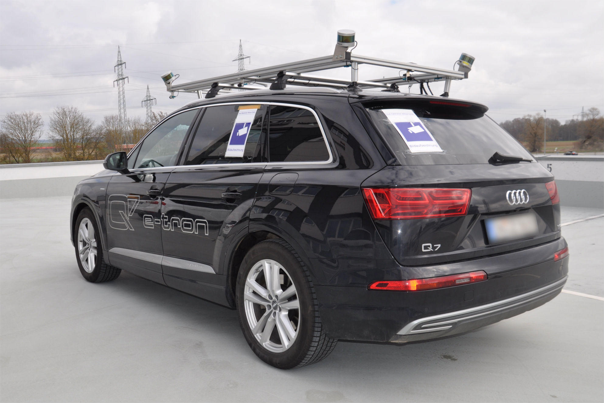
(a) Audi Q7 e-tron

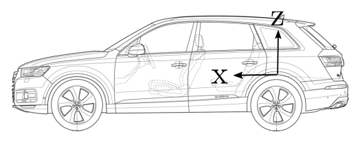
(b) Global reference frame

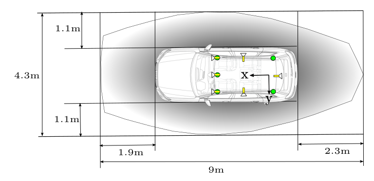
(c) LiDAR blind spots (shaded). Sensor placement is shown in yellow (camera) and green (LiDAR)

Figure 2:

We collected data using an Audi Q7 e-tron equipped with six cameras and five Velodyne VLP-16 sensors (see Tables 2, 3, and 4). In addition to the camera and LiDAR data from our sensor suite, we also recorded the vehicle bus data. Figure 2(a) shows the vehicle used for data collection. The sensor configuration and the frame of reference $\bm{g}$ are visualized in Figure 2(b). The $y$-axis passes through the highest points on the rear wheel arches. The poses of the camera and LiDAR sensors are given with respect to this frame of reference.

Sensor	Location	Type
Camera	Front-center	Sekonix SF3325-100
Camera	Front-left	Sekonix SF3324-100
Camera	Front-right	Sekonix SF3324-100
Camera	Side-left	Sekonix SF3324-100
Camera	Side-right	Sekonix SF3324-100
Camera	Rear-center	Sekonix SF3324-100
LiDAR	Front-center	Velodyne VLP-16
LiDAR	Front-left	Velodyne VLP-16
LiDAR	Front-right	Velodyne VLP-16
LiDAR	Rear-left	Velodyne VLP-16
LiDAR	Rear-right	Velodyne VLP-16

Table 2: Sensor suite

	SF3225-100	SF3224-100
Horizontal FOV	60°	120°
Vertical FOV	38°	73°
Diagonal FOV	70°	146°
Sensor	Onsemi AR0231	Onsemi AR0231
Resolution	1928 x 1208 (2MP)	1928 x 1208 (2MP)
Colour Filter Array	RCCB	RCCB

Table 3: Camera specifications

	VLP-16
Azimuthal FOV	360°
Vertical FOV	30° (+15° to -15°)
Channels	16
Vertical resolution	2°
Frequency	5-20Hz (10Hz used for A2D2)
Range	up to 100m
Rate	up to $\sim$300,000 points/second

Table 4: LiDAR specifications [22]

3.1.1 Sensor Setup

We chose to mount the sensors on the roof of the vehicle with the aim of obtaining $360\degree$ environmental coverage, and to be symmetric with respect to the $x$-$z$-plane. The number of sensors was limited by data recording bandwidth. Three fisheye (120° horizontal FOV) cameras provide views to the left, right, and rear of the vehicle. More emphasis was put on the front view which was covered with three cameras: a pair of fisheye cameras mounted on the front-left and front-right of the roof, and a rectilinear (60° horizontal FOV) camera mounted between them to provide a more detailed and less distorted view. LiDAR sensors were placed at each corner of the setup and above the front center camera. Figure 2(c) shows the described sensor placement.

After fixing the sensor locations, the camera and LiDAR sensor orientations were optimized manually by visualizing the covered 3D region in CAD software. The goal of this process was to minimize the blind spot around the vehicle while maximizing camera and LiDAR field of view overlap. Figure 2(c) depicts the blind spot of the LiDAR sensors, evaluated at the ground plane. Outside the LiDAR blind spot, the fields of view of the cameras and the LiDAR sensors largely overlap (over 90 %). This is demonstrated visually in the upper panel of Figure 3.

3.1.2 Sensor Calibration/Registration

The sensors were mounted on the vehicle as detailed in Section 3.1.1 and measurements were made of their poses. In-situ calibration was still required, especially to account for error in measuring sensor angles.

Firstly, the measured pose of the front-center LiDAR sensor with respect to the reference frame was assumed to be accurate. Using it as a reference, all remaining sensor poses were determined relative to this LiDAR.

Secondly, we performed LiDAR to LiDAR mapping. To do so, LiDAR data was recorded in a static environment, with no dynamic objects. During data collection the vehicle was also stationary. An ICP-based registration [23] was performed for determining the relative pose of the LiDAR sensors with respect to each other.

Thirdly, intrinsic camera calibration was performed for all cameras using 2D patterns (checkerboards).

Finally, the LiDAR to camera mapping was determined as follows: Using a recording with our data recording vehicle in motion (see Section 3.3), a large combined LiDAR point cloud was computed using ego-motion correction based on the bus data and then an ICP-based open-loop SLAM [24] (see lower panel of Figure 3). Given extrinsic camera parameters and using interpolation, a depth image as seen by the respective camera can be computed. Keeping the measured camera positions fixed, the camera angles were determined by optimizing for edge correspondence in the depth and RGB camera images. The top panel of Figure 3 shows LiDAR points projected onto camera images using the resulting mappings.

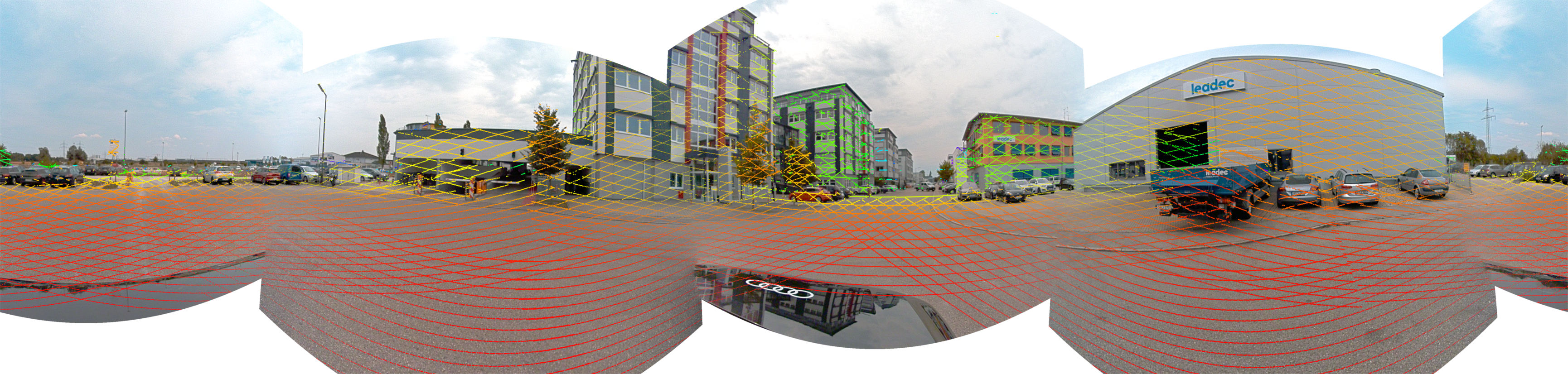
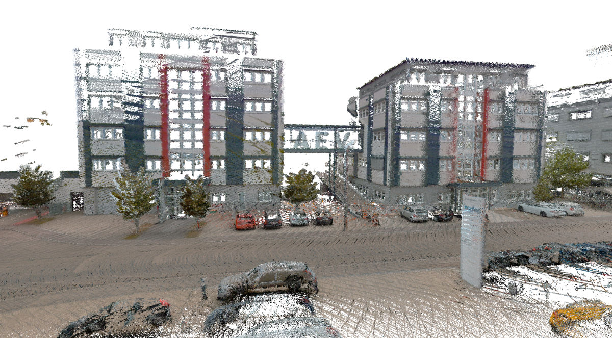
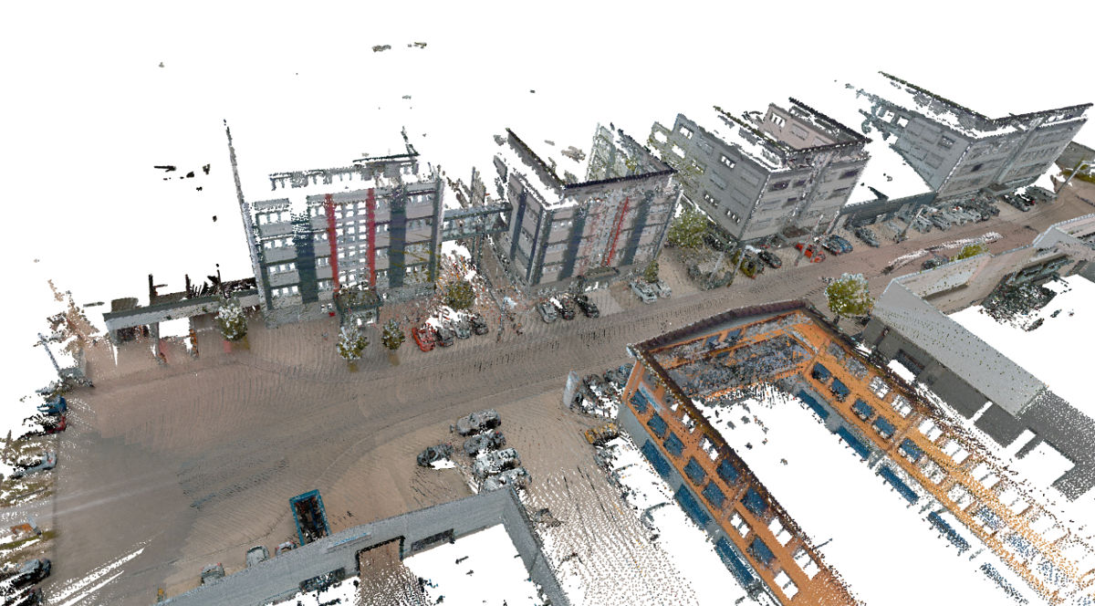
Figure 3: Upper panel: Mapping of LiDAR points onto stitched camera images. Lower panels: colored 3D maps generated from a 30 second sequence using an ICP-based open-loop SLAM.

The result of the calibration is given in a configuration file containing:

• a view, $\bm{v}$, for each sensor as well as the global frame of reference of the vehicle. Each view describes the pose of a sensor with respect to the reference frame, and is given by a tuple of three vectors so that $\bm{v}=(\bm{o},\bm{x},\bm{y})$. The vector $\bm{o}\in\mathbb{R}^{3}$ specifies the Cartesian coordinates (in meters) of the origin of the sensor. $\bm{x},\bm{y}\in\mathbb{R}^{3}$ are unit vectors pointing in the direction (in Cartesian coordinates) of the sensor’s $x$-axis and the $y$-axis. The $z$-axis of the sensor completes an orthonormal basis and thus is obtained by the cross-product $\bm{z}=\bm{x}\times\bm{y}$.

• the following parameters for each camera sensor:

  • $\bm{K}\in\mathbb{R}^{3\times 3}$ – the intrinsic camera matrix of the original (distorted) camera image

  • $\bm{M}\in\mathbb{R}^{3\times 3}$ – the intrinsic camera matrix of the undistorted camera image

  • $\bm{d}\in\mathbb{R}^{4}$ – distortion parameters of the original (distorted) camera image

  • $\bm{r}\in\mathbb{N}^{2}$ – resolution (columns, rows) of undistorted as well as original camera image

  • $L\in\{\mbox{Fisheye},\mbox{Wide-angle}\}$ – type of lens.

3.1.3 Vehicle Bus Data

In addition to camera and LiDAR data, the vehicle bus data were recorded. It is stored in a json-file, which contains the bus signals themselves as well as the corresponding timestamps and units. The signals comprise, e.g., acceleration, (angular) velocity, and GPS coordinates,brake pressure, pitch and roll angles; see Figure 4.

By including vehicle bus data we not only allow A2D2 to be used for imitation (end-to-end) learning research, but also enable reinforcement learning approaches as described in [25].

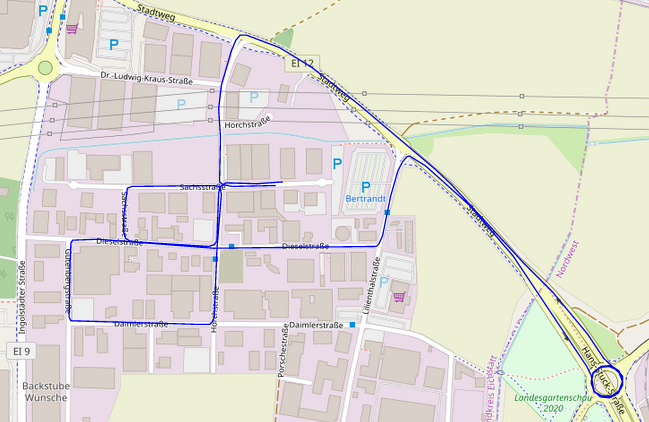
(a) GPS coordinates

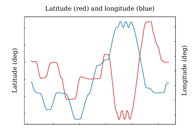
(b) Degree of latitude/longitude

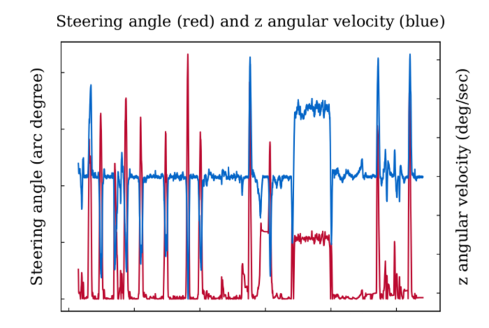
(c) Steering angle and z angular velocity

Figure 4: Three vehicle bus signals are depicted over time. In (a), the GPS signal values are projected onto a map. A roundabout is visible in the lower right corner. This roundabout corresponds to the oscillating part of the longitude and latitude plot (b) as well as the nearly constant part in the plot of steering angle and z angular velocity (c).

3.2 Anonymization

Due to recent privacy laws and regulations we utilized a state-of-the-art semantic segmentation network to blur license plates and heads of pedestrians. This was done for both annotated and un-annotated data (more than 400,000 images).

3.3 Unlabelled Sequence Data

We recorded three urban sequences in Gaimersheim, Munich, and Ingolstadt. These sequences, containing closed loops, are provided as 392,556 unlabelled images (total from all six cameras), together with corresponding LiDAR and bus data. The sequences consist of 94,221, 164,823, and 133,512 images with corresponding timestamps, respectively. As mentioned in Section 2.2, these data are useful for research in end-to-end autonomous driving, depth prediction from mono/stereo images or videos [26, 27], and SLAM. The latter was used for computing the LiDAR-to-camera map in Section 3.1.2, see also Figure 3.

3.4 Data Labels

3.4.1 Semantic Annotations

A2D2 includes images from different road scenarios such as highway, country, and urban. In total, 41,277 camera images are semantically labelled. Of these, 31,448 labels are for front-center camera images, 1,966 for front-left, 1,797 for front-right, 1,650 for side-left, 2,722 for side-right, and 1,694 for rear-center. Each pixel is assigned to a semantic class.

Where multiple instances of the same class of traffic participant (pedestrian, cyclist, car, or truck) share a boundary, they are differentiated using subclasses such as car1, car2, etc. As shown in Figure 5 this only applies to adjacent instances. Therefore the fact that our semantic segmentation taxonomy has classes car[1-4] does not imply that there is a maximum of 4 cars per image.

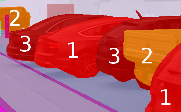
Figure 5: Multiple adjacent car instances. Starting from the right of the above figure, cars 1, 2, and 3 must all have different semantic classes because they share a boundary. The next car to the left can be assigned ‘Car 1’ because it does not share a boundary with any other ‘Car 1’ instance.

In total, there are 38 classes in our semantic segmentation schema. The lower panel of Figure 7 shows these classes along with the distribution of pixels in our dataset. The number of instances of traffic participants annotated with semantic labels in our dataset are depicted in the upper-right panel of Figure 7. Predictably, the traffic participant instance counts are dominated by cars, trucks, and pedestrians.

We also provide LiDAR point clouds for 38,481 semantically labelled images. The 3D semantic labels are obtained by mapping the 3D points to the semantic segmentation images using the LiDAR to camera mapping described in Section 3.1.2.

3.4.2 Instance Segmentation Annotations

We generated instance segmentation annotations from all semantic segmentation annotations. These instance annotations are available for all classes which represent traffic participants such as pedestrians, cars, etc.

3.4.3 3D Bounding Boxes

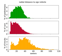
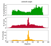
Figure 6: Distributions of radial distances and azimuthal angles for pedestrian, car, and truck bounding box object classes

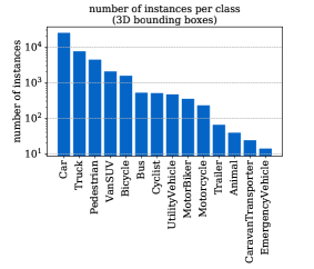
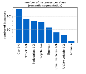
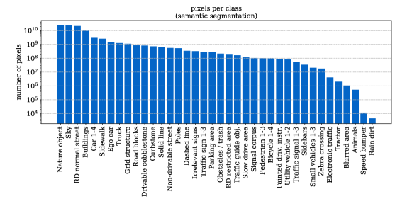
Figure 7: Number of 3D bounding box instances per class, number of traffic participant instances per class (semantic segmentation), semantic segmentation pixel counts per class. Note that “Cyclist” and “MotorBiker” stand for a person including the corresponding vehicle.

For 12,497 of the front-camera frames with semantic annotation, we also provide 3D bounding boxes for a variety of vehicles, pedestrians, and other relevant objects. Figure 7 (top left) shows the full list of annotated classes, along with the number of instances of each class in A2D2. Where objects are partially occluded, human annotators estimated the bounding box to the best of their ability. Examples of this can be seen in the second panel of Figure 1.

3D bounding boxes were annotated in LiDAR space. To do so, we first combined the point clouds from all LiDARs, then culled them to the view frustrum of the front-center camera. Therefore, we provide 3D bounding boxes for the points within the field of view of the front-center camera.

LiDAR point clouds are sparse relative to images. As a result, distant or small objects may not be represented by (m)any points. Since the 3D bounding boxes are derived from LiDAR point clouds, objects may be visible in images but lack corresponding 3D bounding boxes.

Figure 6 (left) shows the distributions of the radial distances to the ego vehicle of the 3D bounding boxes in our dataset for three classes: pedestrians, cars, and trucks. As one may expect, trucks, being physically larger than cars and pedestrians, have a higher optical cross section, and are thus seen and annotated in the LiDAR point clouds to a farther distance.

Although cars are metallic and larger than pedestrians, Figure 6 (left) shows that the distribution of annotated cars drops off quicker with distance than the distribution of annotated pedestrians. A possible explanation for this would be that the distributions of the annotations largely reflect the real world distributions, i.e., the percentage of cars at long range really is smaller than the percentage of pedestrians at long range. This seems unlikely since A2D2 contains recordings from highways and country roads, where we expect many distant cars. A more plausible explanation relies on the fact that LiDAR visibility is not determined solely by optical cross section, but also by occlusion, which is affected by the size, shape, and spatial distribution of objects. Since cars are generally on roads, they tend to be almost directly ahead of the ego vehicle (see right panels of Figure 6). Thus they often occlude other cars rather than pedestrians, the azimuthal distribution of which is more even as shown in Figure 6 (right). This might explain why the distribution of annotated cars falls off quicker with distance than the one for pedestrians.

The same argument does not hold for trucks, despite the fact that they are also mostly directly ahead the ego vehicle (see Figure 6). They are far less common than cars in A2D2 as depicted in the upper panels of Figure 7 (note the logarithmic $y$-axes). This suggests that potential occluding objects are usually not other trucks. That being the case, since trucks are wider and taller than other vehicles, they are less likely to be fully occluded so that they can be perceived to a farther distance.

3.5 Tutorial

Since our aim is to provide a valuable resource to the community, it is important that A2D2 be easy to use. To this end we provide a Jupyter Notebook tutorial with the download, which details how to access and use the dataset.

4 Experiment: Semantic Segmentation

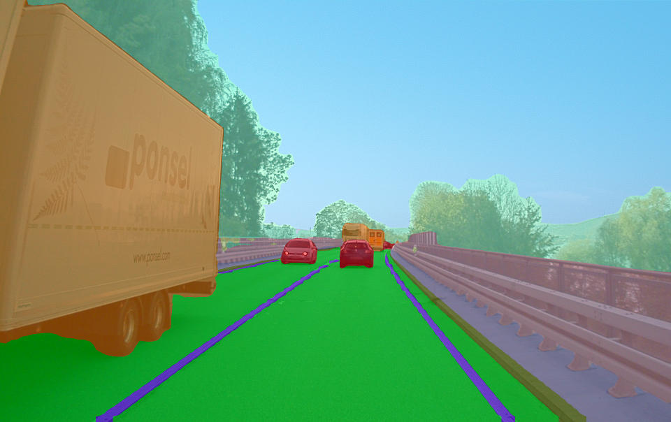
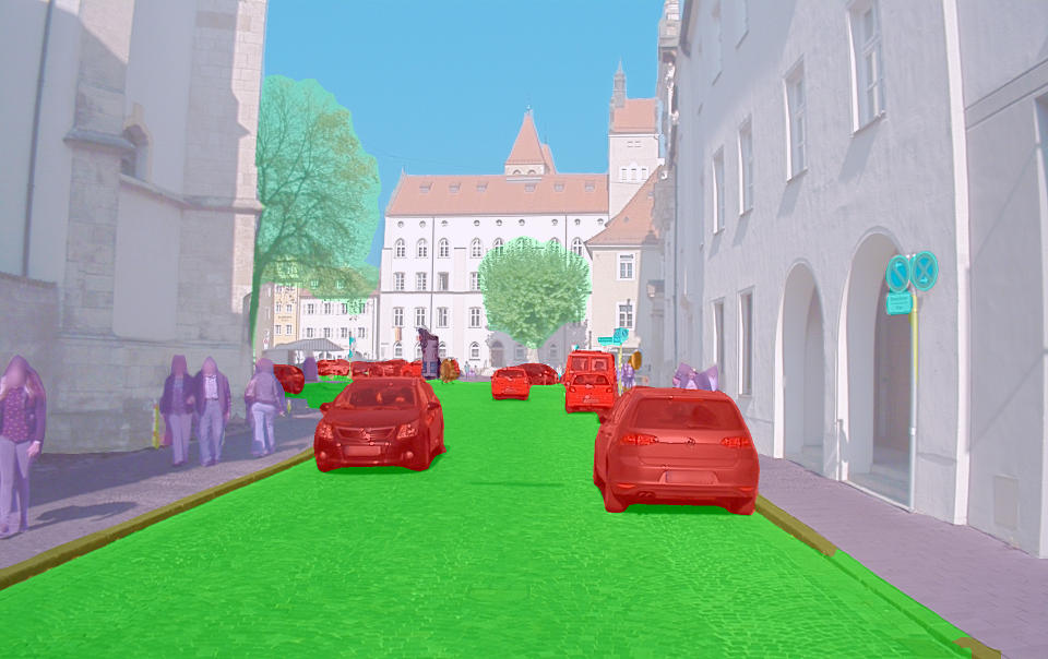
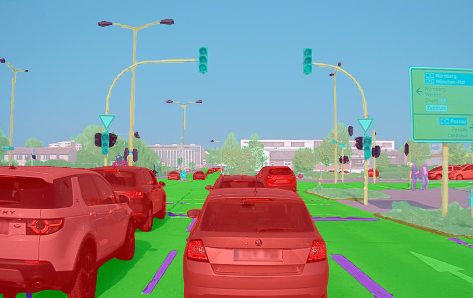
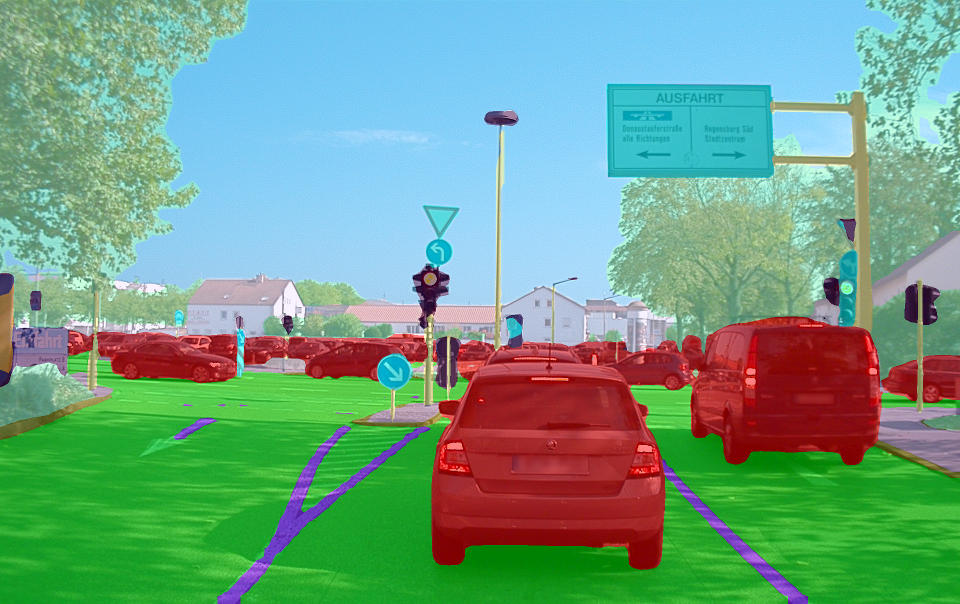
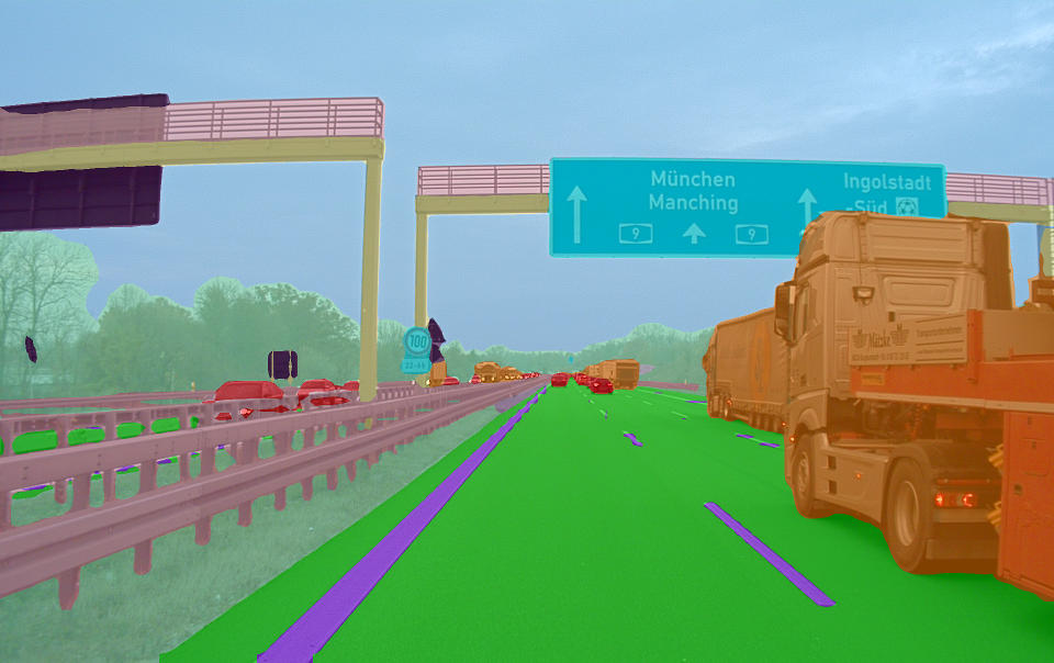
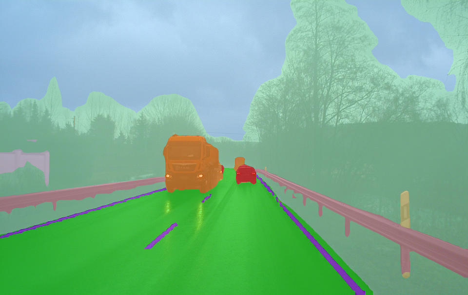
Figure 8: Visual result on test set images of different scenarios

In this section we present the results of training and evaluating a semantic segmentation network on A2D2. In order to establish baseline results, our experiment follows state-of-the-art methods [28, 29], training a fully convolutional network to classify each pixel within an image.

For our experiments, we used 40,030 RGB images with a resolution of $1920\times 1208$ pixels. We split the data into train (28,015 images), validation (4,118), and test (7,897) sets. The experiments were conducted for 18 classes of interest, and an additional background class. These 19 classes were chosen to be as similar as possible to the Cityscapes taxonomy, and were generated by merging similar classes in our 38-class taxonomy. Random cropping, brightness, contrast, and flipping augmentations were applied. As is standard practice, we use mean Intersection over Union (IoU) to evaluate the performance of the model.

4.1 Baseline Results

The network architecture used ResNet-101 [30] as the encoder and the pyramid scene parsing network [31] module as the decoder. The encoder was initialized with weights from ImageNet pre-training. We trained the network using stochastic gradient descent with momentum. The initial learning rate was 0.01 and the momentum parameter was 0.9. The learning rate was decreased polynomially during training. The feature map of the last encoder layer has spatial dimensions $\frac{1}{16}$ those of the input image. This model achieves a mean IoU over the 18 foreground classes of 71.01% on the test set, as shown in Table 5. Figure 8 shows some visual examples of the network output.

Architecture/Training	Mean IOU
Baseline (ResNet-101 + PSP-Net)	71.01%
With pre-trained weights (ResNet-50 + PSP-Net)	68.40%
Without pre-trained weights (ResNet-50 + PSP-Net)	65.31%
With anonymized images (ResNet-101 + PSP-Net)	70.94%

Table 5: Evaluation results on the test set

4.2 Usage of Pre-Trained weights

We assess the influence of ImageNet pre-training versus random weight initialization. The network architecture is similar to the baseline experiment, but the encoder module is replaced by ResNet-50, and the final encoder layer spatial dimensions are $\frac{1}{8}$ those of the input image. The training algorithm and hyperparameters are the same as for the baseline experiments with the only exception that the initial learning rate is $1.0\times 10^{-4}$ for the network with pre-trained weights. The mean IoU evaluation results are shown in Table 5. The model with pre-trained weights achieves a better result.

4.3 Training With Anonymized Images

The results which we have discussed thus far apply to models trained on images which were not anonymized. Since legal requirements require that our dataset be anonymized prior to public release, we investigate the effect of anonymization on performance. To do this we trained our network with anonymized images, where faces and vehicle number plates were blurred. The network architecture and experimental setup are the same as in the baseline experiment, with the encoder once again initialized with ImageNet pre-trained weights. The model achieves a mean IoU of 70.94% on the test set, which is very similar to the baseline result, and does not immediately suggest that anonymization has an adverse effect on the semantic segmentation task. Table 5 shows the results of all of our experiments.

5 Conclusions and Outlook

We provide a commercially usable dataset, which includes camera, LiDAR and bus data recorded from a Audi Q7 e-tron. The data from six cameras and five LiDAR sensors are registered to a global reference frame and include precise timestamps. Rich data is provided, in particular full $360\degree$ sensor coverage of the vehicle environment. We have strived to make A2D2 as accessible and easy to use as possible (license, privacy concerns, interactive tutorial), with the end goal of advancing state-of-the-art commercial and academic research in computer vision, machine learning, and autonomous driving.

We expect to continuously update A2D2 in line with current frontiers in research. Indeed, instance segmentation annotations were not included in the initial public release, but are now available for download. Furthermore we plan to define benchmarks and challenges to allow researchers to easily and fairly compare their algorithms. To this end, we have labeled a test set of $\sim$10K images with semantic segmentation annotations, and are currently exploring how best to allow the community to benchmark against this ground truth.

6 Acknowledgments

We would like to thank Josua Schuberth, Sirinivas Reddy Mudem, Kevin Michael Bondzio, Yunlei Tang, Ajinkya Khoche, Christopher Schmidt, Sumanth Venugopal and Sah Surendra for their help in checking the quality of the dataset. In addition, we would like to thank E.S.R. Labs AG for their help in developing this dataset.

References

- [1] Andreas Geiger, Philip Lenz, Christoph Stiller, and Raquel Urtasun. Vision meets robotics: The KITTI dataset. The International Journal of Robotics Research, 32(11), 2013.
- [2] Peng Wang, Xinyu Huang, Xinjing Cheng, Dingfu Zhou, Qichuan Geng, and Ruigang Yang. The apolloscape open dataset for autonomous driving and its application. IEEE Transactions on Pattern Analysis and Machine Intelligence, 2019.
- [3] Holger Caesar, Varun Bankiti, Alex H Lang, Sourabh Vora, Venice Erin Liong, Qiang Xu, Anush Krishnan, Yu Pan, Giancarlo Baldan, and Oscar Beijbom. nuScenes: A multimodal dataset for autonomous driving. arXiv preprint arXiv:1903.11027, 2019.
- [4] Pei Sun, Henrik Kretzschmar, Xerxes Dotiwalla, Aurelien Chouard, Vijaysai Patnaik, Paul Tsui, James Guo, Yin Zhou, Yuning Chai, Benjamin Caine, et al. Scalability in perception for autonomous driving: Waymo open dataset. arXiv, 2019.
- [5] Andreas Geiger. Are we ready for autonomous driving? The KITTI vision benchmark suite. In Proceedings of the 2012 IEEE Conference on Computer Vision and Pattern Recognition (CVPR), CVPR, 2012.
- [6] Marius Cordts, Mohamed Omran, Sebastian Ramos, Timo Rehfeld, Markus Enzweiler, Rodrigo Benenson, Uwe Franke, Stefan Roth, and Bernt Schiele. The cityscapes dataset for semantic urban scene understanding. In Proceedings of the IEEE conference on computer vision and pattern recognition, 2016.
- [7] Gerhard Neuhold, Tobias Ollmann, Samuel Rota Bulò, and Peter Kontschieder. The Mapillary Vistas dataset for semantic understanding of street scenes. In ICCV, 2017.
- [8] Fisher Yu, Wenqi Xian, Yingying Chen, Fangchen Liu, Mike Liao, Vashisht Madhavan, and Trevor Darrell. BDD100K: A diverse driving video database with scalable annotation tooling. arXiv preprint arXiv:1805.04687, 2018.
- [9] Daniel Munoz, J. Andrew Bagnell, Nicolas Vandapel, and Martial Hebert. Contextual classification with functional max-margin markov networks. 2009 IEEE Conference on Computer Vision and Pattern Recognition, 2009.
- [10] Bastian Steder, Michael Ruhnke, Slawomir Grzonka, and Wolfram Burgard. Place recognition in 3D scans using a combination of bag of words and point feature based relative pose estimation. 2011 IEEE/RSJ International Conference on Intelligent Robots and Systems, 2011.
- [11] Jens Behley, Volker Steinhage, and Armin Cremers. Performance of histogram descriptors for the classification of 3D laser range data in urban environments. In 2012 IEEE International Conference on Robotics and Automation (ICRA), 05 2012.
- [12] Richard Zhang, Stefan Candra, Kai Vetter, and A. Zakhor. Sensor fusion for semantic segmentation of urban scenes. In 2015 IEEE International Conference on Robotics and Automation (ICRA), 05 2015.
- [13] Timo Hackel, N. Savinov, L. Ladicky, Jan D. Wegner, K. Schindler, and M. Pollefeys. SEMANTIC3D.NET: A new large-scale point cloud classification benchmark. In ISPRS Annals of the Photogrammetry, Remote Sensing and Spatial Information Sciences, volume IV-1-W1, 2017.
- [14] Jens Behley, Martin Garbade, Andres Milioto, Jan Quenzel, Sven Behnke, Cyrill Stachniss, and Juergen Gall. SemanticKITTI: A Dataset for Semantic Scene Understanding of LiDAR Sequences. In Proc. of the IEEE/CVF International Conf. on Computer Vision (ICCV), 2019.
- [15] R. Kesten, M. Usman, J. Houston, T. Pandya, K. Nadhamuni, A. Ferreira, M. Yuan, B. Low, A. Jain, P. Ondruska, S. Omari, S. Shah, A. Kulkarni, A. Kazakova, C. Tao, L. Platinsky, W. Jiang, and V. Shet. Lyft Level 5 AV Dataset 2019. https://level5.lyft.com/dataset/, 2019. Accessed: 2019-10-24.
- [16] Mariusz Bojarski, Davide Del Testa, Daniel Dworakowski, Bernhard Firner, Beat Flepp, Prasoon Goyal, Lawrence D. Jackel, Mathew Monfort, Urs Muller, Jiakai Zhang, Xin Zhang, Jake Zhao, and Karol Zieba. End to End Learning for Self-Driving Cars. arXiv e-prints, Apr 2016.
- [17] Yi Xiao, Felipe Codevilla, Akhil Gurram, Onay Urfalioglu, and Antonio M. López. Multimodal end-to-end autonomous driving. arXiv preprint arXiv:1906.03199, 2019.
- [18] Hege Haavaldsen, Max Aasboe, and Frank Lindseth. Autonomous vehicle control: End-to-end learning in simulated urban environments. arXiv preprint arXiv:1905.06712, 2019.
- [19] Wolfgang Hess, Damon Kohler, Holger Rapp, and Daniel Andor. Real-time loop closure in 2D LiDAR SLAM. In 2016 IEEE International Conference on Robotics and Automation (ICRA), 2016.
- [20] Hatem Alismail, L. Douglas Baker, and Brett Browning. Continuous trajectory estimation for 3D SLAM from actuated LiDAR. In 2014 IEEE International Conference on Robotics and Automation (ICRA), 2014.
- [21] Stefan Kohlbrecher, Oskar von Stryk, Johannes Meyer, and Uwe Klingauf. A flexible and scalable SLAM system with full 3D motion estimation. In 2011 IEEE International Symposium on Safety, Security, and Rescue Robotics, 2011.
- [22] Velodyne LiDAR Puck VLP-16 Datasheet. https://velodynelidar.com/downloads.html#datasheets. Accessed: 2019-10-28.
- [23] Paul J. Besl and Neil D. McKay. A Method for Registration of 3-D Shapes. IEEE Transactions on Pattern Analysis and Machine Intelligence, 14(2), 1992.
- [24] Feng Lu and Evangelos Milios. Robot pose estimation in unknown environments by matching 2D range scans. Journal of Intelligent and Robotic systems, 18(3), 1997.
- [25] Pieter Abbeel, Adam Coates, Morgan Quigley, and Andrew Y. Ng. An application of reinforcement learning to aerobatic helicopter flight. In In Advances in Neural Information Processing Systems 19. MIT Press, 2007.
- [26] David Eigen, Christian Puhrsch, and Rob Fergus. Depth map prediction from a single image using a multi-scale deep network. In Z. Ghahramani, M. Welling, C. Cortes, N. D. Lawrence, and K. Q. Weinberger, editors, Advances in Neural Information Processing Systems 27. 2014.
- [27] Nan Yang, Rui Wang, Jörg Stückler, and Daniel Cremers. Deep virtual stereo odometry: Leveraging deep depth prediction for monocular direct sparse odometry. arXiv preprint arXiv:1807.02570, 2018.
- [28] Jonathan Long, Evan Shelhamer, and Trevor Darrell. Fully convolutional networks for semantic segmentation. arXiv preprint arXiv:1411.4038, 2014.
- [29] Liang-Chieh Chen, Yukun Zhu, George Papandreou, Florian Schroff, and Hartwig Adam. Encoder-decoder with atrous separable convolution for semantic image segmentation. In ECCV, 2018.
- [30] Kaiming He, Xiangyu Zhang, Shaoqing Ren, and Jian Sun. Identity mappings in deep residual networks. arXiv preprint arXiv:1603.05027, 2016.
- [31] Hengshuang Zhao, Jianping Shi, Xiaojuan Qi, Xiaogang Wang, and Jiaya Jia. Pyramid scene parsing network. In CVPR, 2017.