Enhancing RBF-FD Efficiency for Highly Non-Uniform Node Distributions via Adaptivity

Abstract

Radial basis function generated finite-difference (RBF-FD) methods have recently gained popularity due to their flexibility with irregular node distributions. However, the convergence theories in the literature, when applied to nonuniform node distributions, require shrinking fill distance and do not take advantage of areas with high data density. Non-adaptive approach using same stencil size and degree of appended polynomial will have higher local accuracy at high density region, but has no effect on the overall order of convergence and could be a waste of computational power. This work proposes an adaptive RBF-FD method that utilizes the local data density to achieve a desirable order accuracy. By performing polynomial refinement and using adaptive stencil size based on data density, the adaptive RBF-FD method yields differentiation matrices with higher sparsity while achieving the same user-specified convergence order for nonuniform point distributions. This allows the method to better leverage regions with higher node density, maintaining both accuracy and efficiency compared to standard non-adaptive RBF-FD methods.

65N12, 65N35.

1 Introduction

In the past two decades, there has been important progress in developing adaptive mesh methods for PDEs. Mesh adaptivity is usually of two types in form: local mesh refinement and moving mesh method.

Radial basis functions (RBFs) have been a popular choice in the development of kernel-based meshless methods for solving partial differential equations (PDEs) numerically. Besides collocation methods, the localized RBF-FD method has gained popularity in recent years due to its many advantages, including numerical stability on irregular node layouts, high computational speed and accuracy, easy local adaptive refinement, and excellent opportunities for large-scale parallel computing.

The idea of RBF and kernel-based differentiation can be traced back to [28], and it was formally introduced as the RBF-FD in [29]. Since then, a significant amount of research has been dedicated towards the robust development of the RBF-FD method [30, 3, 12, 11, 8, 2, 25, 22, 21, 19], as well as its application to various problems in science and engineering [4, 7, 9, 26, 16, 15, 17, 13, 27, 14]. In addition to the RBF-FD method, other collocation methods based on radial basis functions have also been proposed. For example, a global radial basis function collocation method in [5] was successfully applied to solve a computational fluid dynamic problem, and local RBF collocation methods were used to solve the diffusion problem in [6] and Hamiltonian PDEs in [32].

The RBF-FD method is advantageous since it work with scattered nodes, allowing for stencils with different configurations and overcoming the fixed grid/element limitation of conventional numerical methods. Unlike global meshless methods, RBF-FD computes weights locally using RBFs expanded at a fixed number of nearest nodes. Once weights at each node are computed, they can be stored and used for next-step computation, making weight computation a pre-processing step in solving time-dependent PDEs. Furthermore, weight computations at each node are independent processes, making RBF-FD a desirable method for parallel computing.

It has been demonstrated [8, 2] that combining polynomial basis with polyharmonic spline radial basis functions (PHS+Poly) in the RBF-FD formulation leads to considerable improvements in robustness. Key benefits of the PHS+Poly approach include:

1. It is free of shape parameter, simplifying the formulation and eliminating the need for fine-tuning.

2. It is efficient compared to stable RBF-FD formulations based on infinitely smooth RBFs [22].

3. This method ensures accuracy near boundaries without ghost-nodes where stencils become highly one-sided [1].

4. It has the potential to maintain accuracy for large and sparse linear systems.

5. The convergence order depends mainly on the augmented polynomial degree, which determines the stencil size.

Existing convergence theories for scattered nodes require shrinking fill distance and fail to leverage regions of high node density. Numerically, non-adaptive methods using uniform stencil size and polynomial degree may exhibit loss of accuracy in low-density regions while adding unnecessary complexity in high-density regions, decreasing computational efficiency. Rather than a fixed stencil size and augmented polynomial degree, we propose an adaptive RBF-FD algorithm that allows the user to define a global convergence order with respect to the total number of nodes in the domain. The method can efficiently obtain the user-defined convergence order in a highly nonuniform node-layout with a significantly large mesh ratio. Note that the mesh ratio is defined as the fill distance over minimum separating distance, which plays a role similar to mesh ratio in finite element methods.

The rest of the paper is organized as follows. Section 2 discusses the general formulation of RBF-FD and polynomial augmentation, along with some insights for its stable implementation. In Section 3, we provide a precise definition of the global convergence order in a nonuniform node-layout. We also present a method that connects the global convergence order to the required degree of polynomial at a local scale, depending on the local fill distance. This is followed by a discussion of the weight computation approach through the adaptive RBF-FD method. In Section 4, numerical examples are illustrated to show the advantages of the proposed method. Finally, section 5 is the conclusions drawn from our study.

2 RBF-FD approximation

Figure 1: A prototype figure showing centers and local stencil.

We first review the basic RBF-FD method. Let $\Omega\subset\mathbb{R}^{d}$ be a computational domain with a set of distinct scattered nodes $X:=\{\bm{x}_{1},\bm{x}_{2},...,\bm{x}_{N}\}\subset\Omega$. Given a linear differential operator $\mathcal{L}$, we aim to approximate the values of $\mathcal{L}u$ at a center/point of interest $\bm{x}^{c}\in X$ based on the nodal values of $u$ at some stencil or set of neighboring nodes of $\bm{x}^{c}$ in $X$. Figure 1 shows the prototype of the scatter data distribution and local stencil for the point of interest.

Let the stencil of $\bm{x}_{c}$ be denoted by $X_{c}:=\{\bm{x}_{1}^{c},\ldots,\bm{x}_{n_{s}}^{c}\}\subseteq X$, where $n_{s}^{c}$ is the stencil size of $\bm{x}_{c}$. Then, the value of $\mathcal{L}u(\bm{x}_{c})\in\mathbb{R}$ can be approximated by as:

$$\mathcal{L}u(\bm{x}_{c})\approx\sum_{k=1}^{n_{s}^{c}}w_{k}^{c}u\left(\bm{x}_{k}^{c}\right)=\bm{w}_{c}u|_{X_{c}},$$ (1)

where $u|_{X_{c}}:=[u(\bm{x}_{1}^{c}),\ldots,u(\bm{x}_{n_{s}}^{c})]^{T}$ is the nodal values of $u$ evaluated at stencil $X_{c}$. We need to compute the weights $\bm{w}_{c}:=[w_{1}^{c},w_{2}^{c},\ldots,w_{N}^{c}]^{T}$ at $\bm{x}_{c}$ for this finite difference approximation.

In RBF-FD method, interpolants were used as surrogate. Using some symmetric positive definite (SPD) radial basis function $\phi:[0,\infty)\rightarrow\mathbb{R}$, the RBF surrogate interpolates the data at $(X_{c},u|_{X_{c}})\in\mathbb{R}^{d}\times\mathbb{R}$ while keeping function values $u|_{X_{c}}$ as unknown. The RBF-FD weights $\bm{w}_{c}$ are computed by applying $\mathcal{L}$ to the surrogate and, then, evaluating at $\bm{x}_{c}$. This is equivalent to solving:

$$\underbrace{\left[\phi(\|\bm{x}_{i}^{c}-\bm{x}_{j}^{c}\|)\right]_{1\leq i,j\leq n_{s}^{c}}}_{\displaystyle=:A_{c}}\bm{w}_{c}=\underbrace{\left[\mathcal{L}\phi(\|\bm{x}-\bm{x}_{i}^{c}\|)_{|\bm{x}=\bm{x}_{c}}\right]_{1\leq i\leq n_{s}^{c}}}_{\displaystyle=:[\mathcal{L}\phi]_{|\bm{x}_{c}}}.$$ (2)

Since $\phi$ is SPD, $A_{c}$ is SPD and (2) is uniquely solvable. It is shown in [23] that (2) is error optimal in the native space norm corresponding to the radial basis function $\phi$. We refer readers to the article for details.

2.1 RBF-FD using PHS+Poly

In contrast to global meshless methods, the local nature of RBF-FD rules out exponential convergence for approximating functions in certain native spaces. Even with infinitely smooth RBFs, the convergence is limited for RBF-FD by stencil sizes. Motivated by the discussion in [24], we use a conditionally positive definite kernel with finite order of smoothness in the RBF-FD method. For example, we and use a conditionally SPD polyharmonic spline (PHS) kernel:

$$\phi(r)=r^{2m+1},\ m\in N^{+}.$$

To ensure unique solvability, we augment polynomial basis of sufficient degrees to ensure exact reproduction of low order polynomials. To compute RBF-FD weights in (1) by PHS+Poly, the surrogate $I(\mathbf{x})$ now uses RBFs and polynomial basis up to degree $p$ as basis functions:

$$I(\mathbf{x})\approx\sum_{k=1}^{n_{s}^{c}}\lambda_{k}\phi\left(\parallel\bm{x}-\bm{x}_{k}^{c}\parallel\right)+\sum_{{l}=1}^{n_{p}^{c}}\gamma_{{l}}p_{l}(\bm{x}),\quad\bm{x}\in\Omega,$$ (3)

subject to interpolation conditions at data $(X_{c},u|_{X_{c}})\in\mathbb{R}^{d}\times\mathbb{R}$ and constraints

$$\sum_{k=1}^{n_{s}^{c}}\gamma_{l}p_{l}(\bm{x}_{k}^{c})=0,\quad l=1,2,3,...,n_{p}^{c},$$ (4)

where $n_{p}^{c}$ is the number of augmented multivariate polynomial basis and $n_{s}^{c}$ is again the stencil-size of $\bm{x}_{c}$ .

The counterpart to the linear system (2) for RBF-FD using PHS+Poly is given by

$$\begin{bmatrix}A_{c}&P_{c}\\ P_{c}^{T}&O\end{bmatrix}\begin{bmatrix}\bm{w}\\ \bm{w}_{e}\end{bmatrix}=\begin{bmatrix}[\mathcal{L}\phi]_{|\bm{x}_{c}}\\ [\mathcal{L}{p}]_{|\bm{x}_{c}}\end{bmatrix},$$ (5)

which can be interpreted as an equality-constrained quadratic programming problem (see [2] for more details on this). In (5), matrices $A_{c}$ and $[\mathcal{L}\phi]$ are defined as in (2). The $n_{s}^{c}\times n_{p}^{c}$ matrix $P_{c}$ and $n_{p}^{c}\times 1$ vector $[\mathcal{L}{p}]_{|\bm{x}_{c}}$ are given as

$$P_{c}=[p_{j}(\bm{x}_{i}^{c})]_{1\leq i\leq n_{s}^{c},\,1\leq j\leq n_{p}^{c}},\mbox{\quad and \quad}[\mathcal{L}{p}]_{|\bm{x}_{c}}=[\mathcal{L}p_{l}(\bm{x})_{|\bm{x}=\bm{x}_{c}}]_{1\leq l\leq n_{p}^{c}}.$$

From here and on, we drop the super/subscript $c$ from notations for simplicity, and all computations need to be done center by center for all $\bm{x}_{c}\in X$. The number of polynomial basis $n_{p}$ up to degree $p$ in $d$-dimensional is given by

$$n_{p}=C(p+d,d)=\frac{(p+d)!}{p!d!}.$$ (6)

Table 1 lists out polynomial terms for different degrees in some cases in 2D, see [8] for more. For example, $n_{p}=3$ in 2D, corresponds to appending polynomial up to first order.

Table 1: The polynomial basis of different degree for 2D case

Polynomial degree ($p$)	Polynomial basis	$n_{p}=C(p+2,2)=\frac{(p+2)!}{p!2!}$
0	$1$	1
1	$1,x,y$	3
2	$1,x,y,x^{2},y^{2},xy$	6
3	$1,x,y,x^{2},y^{2},xy,x^{3},y^{3},x^{y},xy^{2}$	10

3 Adaptive PHS+Poly RBF-FD methods

Adaptive methods are quite popular in the context of finite element methods (FEM), and many algorithms such as $h$-FEM, $p$-FEM, or $hp$-FEM were proposed. In order to meet a certain order of accuracy throughout the domain, the idea behind adaptivity is to vary parameters affecting the accuracy of the algorithm locally. In this section, we aim to develop an adaptive PHS+Poly RBF-FD scheme that:

1. Achieve the expected order of accuracy in the domain, including evaluation points near boundaries where stencils are highly one-sided.

2. Maintain accuracy and obtain linear systems with higher sparsity for dealing with large-scale problems.

3.1 Polynomial refinement and adaptive stencil size

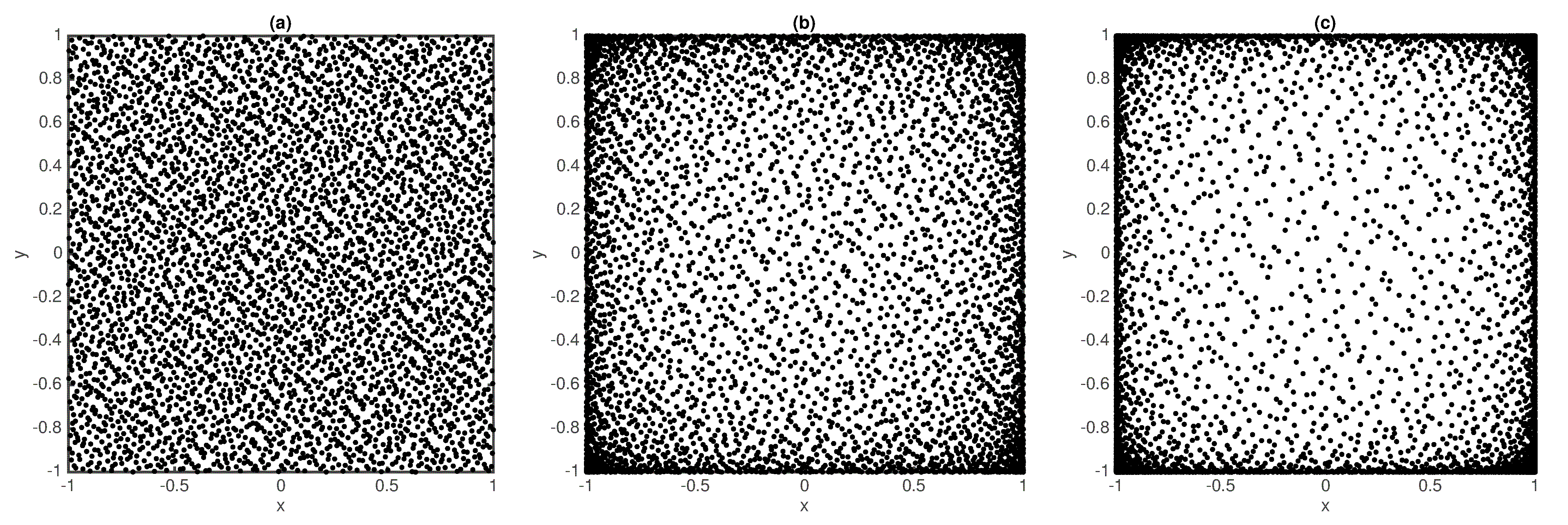
Figure 2: Node distribution under different mesh ratio with $N=4096$ quasi-uniform data points in unit square $[-1,1]^{2}$ with various mesh ratios: (a) $\rho_{X}\approx 1$, (b) $\rho_{X}\approx 10^{2}$, and (c) $\rho_{X}\approx 10^{5}$.

Given a set of $N$ scattered data $X\subset\mathbb{R}^{d}$. Its fill distance and separation distance are given by

$$h_{X,\Omega}:=h_{X}=\sup_{\bm{x}\in\Omega}\min_{\bm{x}_{j}\in X}\|\bm{x}-\bm{x}_{j}\|_{\ell_{2}(\mathbb{R}^{d})},\quad q_{X}:=\frac{1}{2}\min_{i\neq j}\|\bm{x}_{i}-\bm{x}_{j}\|_{\ell_{2}(\mathbb{R}^{d})},$$ (7)

and $\rho_{X}=h_{X}/q_{X}\geq 1$ is the mesh ratio of $X$. A quasi-uniform data set refers to a sequence of data sets where the mesh ratio $\rho_{X}$ remains bounded for all $N$ as $X$ refines with increasing $N$. The number of nodes $N$ typically scales as $N\sim q_{X}^{-d}$, where $\sim$ means proportional up to a constant. Figure 2 shows node distributions of $N=$ 4,096 under mesh ratios $\rho_{X}=$ 1, $10^{2}$, and $10^{5}$, respectively.

Data sets with large mesh ratios will be considered highly nonuniform, which is the target of our proposed adaptive approach. Nonuniform nodes are often associated with rapidly varying regions of a function or other physical quantities. For example, the adaptive node distributor in NodeLab [18, 10] can generate a sequence of scattered data sets with large mesh ratios $\rho$ that are denser in user specified problematic spatial regions. The folklore is that high point density will induce a smaller stencil radius even if the stencil size $n_{s}$ is fixed at a constant for all centers. Yet this could yield an inefficient algorithm, which we aim to improve upon.

In the RBF-FD method, for quasi-uniform node distribution, the convergence can be estimated in a straightforward manner. Suppose we want to approximate a $k$-th order differential operator $\mathcal{L}$ by PHS+Poly RBF-FD with appended polynomial up to degree $p$. According to results in [8, 2], for a quasi-uniform node distribution, the convergence order of a RBF-FD method is $\sim h_{X}^{p-k+1}$. It has been found in [8, 2] that the convergence order of PHS+Poly RBF-FD was governed by the degree of augmented polynomial $p$, while the smoothness order of the PHS has a marginal effect on the accuracy and no influence on the order of convergence.

Let us first consider an ideal quasi-uniform point set $X$ of $N$ points in $\Omega$ (with minimal mesh ratio) that has an equispaced fill distance proportional to

$$h_{e,\Omega}=\left(\frac{\text{Vol}(\Omega)}{N}\right)^{1/d}.$$

Suppose we want to design an adaptive PHS+Poly RBF-FD algorithm to approximate a $k$-th order differential operator $\mathcal{L}$ with user-specified $g^{th}$ order convergence. The approximation error is then expected to behave like $\varepsilon\sim h_{e,\Omega}^{g}$. Moving to highly nonuniform nodes with large mesh ratio, we define global convergence with respect to $h_{e,\Omega}$ by formulating an adaptive RBF-FD approach with adaptive polynomial refinement.

For a general data set $X\subset\Omega$ with no constraint on its mesh ratio, let $X_{c}\subset X$ denote the stencil associated with the point of interest $\bm{x}^{c}\in X$, and $\Omega_{c}=conv(X_{c})$ be its associated local sub-domain. Also let $\Omega_{c}:=conv(X_{c})$ be its local sub-domain defined by convex hulls and $h_{X,\Omega_{c}}$ be the associated local fill distance. If we employ a $g^{th}$-order RBF-FD scheme at this center, then the local error $\varepsilon_{c}$ will reduce as

$$\varepsilon_{c}\sim h_{X}^{g}=(\rho_{X}q_{X})^{g}\sim\rho_{X}^{g}N^{-g/d}.$$

For uniform node with $\rho_{X}=1$, the last factor $N^{-g/d}\sim h_{e}^{g}$ is exactly what we expect from a $g^{th}$-order finite difference scheme. In cases when $\rho_{X}\gg 1$, the asymptotic convergence rate remains order-$g$ but with a large leading constant $\rho_{X}^{g}$ that reduces the final accuracy in the error bound. To sum up, the large mesh ratio of highly nonuniform nodes weakens the approximation accuracy in terms of magnitude, but not order of convergence.

Since the (local) convergence order by PHS+Poly RBF-FD algorithm is decided by the polynomial order and (local) fill distance $h_{X,\Omega_{c}}$, we can obtain $g^{th}$-convergence by adaptively varying the degree $p_{c}$ of augmented polynomial order that satisfies:

$$h_{X,\Omega_{c}}^{p_{c}-k+1}=h_{e,\Omega}^{g}.$$ (8)

In this context, non-adaptive standard approach takes $p_{c}-k+1=g$ for all centers $\bm{x}^{c}$. Note that, by the definition of fill distance, at least one of these local fill distance $h_{X,\Omega_{c}}$ must coincide with the global fill distance $h_{X,\Omega}$, that acts as an upper bound. This particular stencil is the limiting factor for the final accuracy.

Given the equispaced fill distance $h_{e,\Omega}$ (or $\text{Vol}(\Omega)$ and $N$), the local fill distance $h_{X,\Omega_{i}}$ for each point of interest, and the order $k$ of the differential operator $\mathcal{L}$, the local polynomial orders for $g^{th}$ convergence can be determined from (8) as:

$$\mathbb{N}\ni p_{c}\geq g\frac{\log_{10}h_{e,\Omega}}{\log_{10}h_{X,\Omega_{c}}}+k-1.$$ (9)

For quasi-random nodes with small mesh ratio, we expect $h_{X,\Omega_{i}}\approx h_{e,\Omega}$ and $p_{c}$ in (9) simplifies to

$$p=g+k-1\qquad\text{or}\qquad g=p-k+1.$$ (10)

Our adaptive scheme aligns with existing non-adaptive methods [8, 2] in this case. By adaptively determining $p_{c}$ from (9), we can achieve better accuracy for highly nonuniform nodes.

The stencil size $n_{s}$ also impacts the accuracy and convergence of RBF-FD. Studies have shown that when the polynomial order is sufficiently high, increasing $n_{s}$ beyond the number of polynomial basis functions $n_{p}$ does not significantly improve accuracy or convergence order, see [8, 2]. For lower-order polynomials, increasing $n_{s}$ can improve accuracy but convergence order remains unchanged. This independence on stencil size is important for our adaptive scheme. In denser regions, we can use a smaller polynomial degree (and $n_{s}$) without significant losses. A stencil size of $n_{s}=n_{p}$ is suggested in [8, 2] for distributions with ghost nodes outside the boundary to avoid stagnation error. Using PHS only without appended polynomials in RBF-FD, stagnation errors stem mainly from boundary errors. However, with polynomial augmentation and $n_{s}\geq 2n_{p}$, RBF-FD remains free from stagnation error.

Based on these findings, we propose: after computing $p_{c}$ from (9) for a user-specified order of convergence $g$, we use $n_{s}=2n_{p}+1$ as suggested in [8, 2] to ensure the solvability and the stability of our algorithm. Since oversized stencil size does not improve accuracy, a smaller $n_{s}$ can be used in regions with smaller $h_{X,\Omega_{i}}$without significantly affecting accuracy or stability. Figure 3 illustrates our proposed adaptive PHS+poly RBF-FD scheme. Since the computational cost of the RBF-FD depends on the stencil-size $n_{s}$, using smaller local $n_{s}$ in denser regions can improve efficiency. The resulting FD-differentiation matrix also enjoys higher sparsity. Algorithm 1 summarizes the RBF-FD weight computation using our adaptive PHS+Poly RBF-FD scheme.

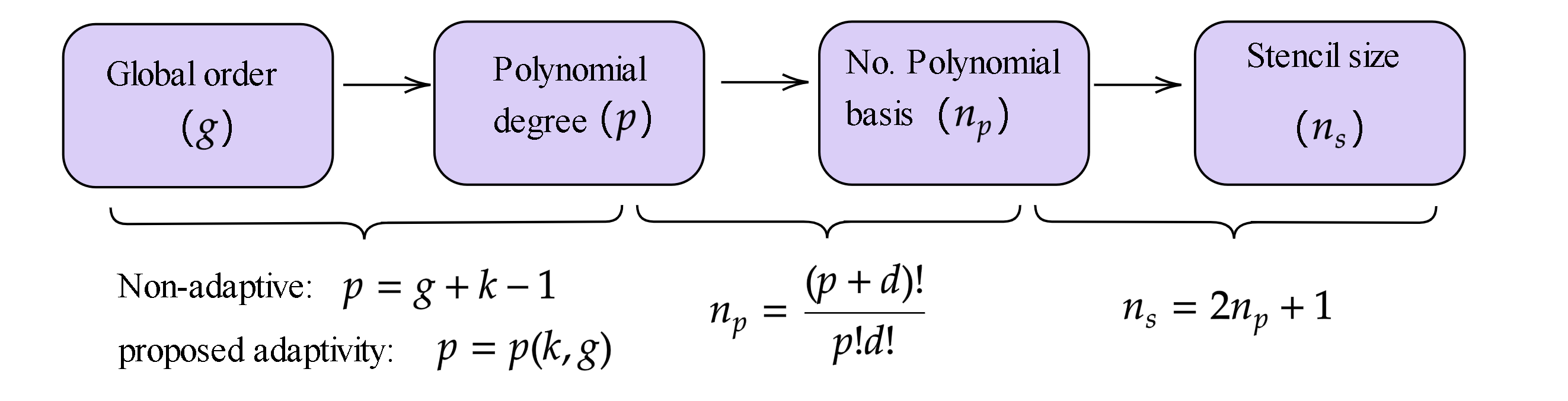
Figure 3: The process of achieving a global order of convergence in an PHS+Poly RBF-FD formulation. The order of convergence $g$ input by the user. The algorithm decides the degree of polynomial to be augmented, which also gives the number of polynomial terms required ($n_{p}$) and consequently the stencil size ($n_{s}$).

Algorithm 1: Adaptive PHS+Poly RBF-FD method

1:procedure Input($g\in\mathbb{N}$, $X\subset\Omega\subset\mathbb{R}^{d}$) $\triangleright$ Input expected order and nodes

2:    Compute total number of nodes $N=|X|$

3:    Compute $h_{e,\Omega}=\left({\frac{Vol(\Omega)}{N}}\right)^{1/d}$

4:    Determine maximum stencil size $n_{s,\max}$

5:    for each point of interest $\bm{x}_{c}$  do

6:        Find $n_{s,\max}$ – nearest neighbors for each $\bm{x}_{c}$ $\triangleright$ We have used knn-search

7:        Find $h_{X,\Omega_{c}}$ $\triangleright$ Estimate local fill-distance

8:        $p_{i}=\lceil g\frac{\log_{10}h_{e,\Omega}}{\log_{10}h_{X,\Omega_{c}}}+k-1\rceil$ $\triangleright$ Polynomial degree required to maintain order $g$

9:        $n_{p}=C(p+d,d)=\frac{(p+d)!}{p!d!}$ $\triangleright$ Number of polynomial basis

10:        $n_{s}=2n_{p}+1$ $\triangleright$ Stencil size just enough to support the polynomial $p$

11:        $r=\sqrt{(x^{2}+y^{2})}$

12:        $A0=r^{m}$ $\triangleright$ The RBF interpolant

13:        $RHS0=[rhs_{L}]$ $\triangleright$ The RHS column in equation (1)

14:        $A=A0+Poly(p)$ $\triangleright$ The RBF interpolant after augmenting polynomial of degree $p$

15:        $RHS=RHS0+Poly(p)$ $\triangleright$ Adding corresponding polynomial of degree $p$

16:        $w_{L}=A/RHS$ $\triangleright$ Solve the linear system for weights

17:        $w_{L}=w(1:n_{s})$ $\triangleright$ Ignore the weights corresponding to polynomial augmentation     

18:    end

19:end

4 Numerical experiments

This section presents four numerical experiments demonstrating the performance of the proposed adaptive method. First, illustrative examples show the key concepts and behavior of the adaptive method. Then, a benchmark problem evaluates accuracy and convergence. Finally, real-world applications demonstrate effectiveness for both steady and time-dependent problems, showing the method’s robustness, accuracy, and adaptivity.

4.1 Example 1: Performance of the proposed adaptive method

In the first test, we investigate the proposed adaptive PHS+Poly RBF-FD scheme by solving an elliptic partial differential equation in domain $\Omega=[-1,1]^{2}$ with boundary $\Gamma_{1}:\{(x,y)|-1\leq x\leq 1,y=1\}$ and $\Gamma_{2}:=\partial\Omega\setminus\Gamma_{1}$. The problem is set up as follows: find $u(x,y)$ such that

$$\begin{aligned} -\nabla^{2}u(x,y)&=f(x,y),\qquad\qquad(x,y)\in\Omega,\end{aligned}$$

subject to boundary conditions

$$\begin{aligned} \frac{\partial u(x,y)}{\partial\bm{n}}&=\cos(x^{2}+y),\qquad(x,y)\in\Gamma_{1},\\ u(x,y)&=\sin(x^{2}+y),\qquad(x,y)\in\Gamma_{2}.\end{aligned}$$

The analytical solution and the source term are given, respectively, as

$$\begin{aligned} u(x,y)=\sin(x^{2}+y),\ f(x,y)=-2\cos(x^{2}+y)-(4x^{2}+1)\sin(x^{2}+y).\end{aligned}$$

We test two quasi-uniform point distributions with $N=2500$ under two mesh ratio, see Figure 4. Nonuniform distributed nodes with large mesh ratio are obtained by the transformation $z=\sin\left((\pi z)/2\right)$ in all coordinates.

For a target convergence rate of $g=3$, Figure 5 (a-b) show the sparsity patterns and eigenvalues of $\mathcal{L}$ of the globally assembled differentiation matrix for uniform nodes and Figure 5 (c-d) for nonuniform nodes. Recall that the adaptive method is equivalent to the standard RBF-FD on uniform node distribution. From Figure 5 (a,c), it can be seen that the adaptive method has a smaller bandwidth in the range $[12,15]$ (except near boundaries) compared to the fixed bandwidth $[15]$ for standard RBF-FD. The total nonzero elements are $6.5\times 10^{4}$, an 20% reduction. From Figure 5 (b,d), the real parts of the eigenvalues computed from the differentiation matrix are all non negative, showing that stable approximations can be obtained by our adaptive approach with higher sparsity.

Figure 6 shows the convergence profile of $\ell^{\infty}$-error:

$$\text{$\ell^{\infty}$-error }=\max_{1\leq i\leq N}\big{|}u(x_{i})-\hat{u}(x_{i})\big{|},$$

versus $N^{1/d}$ for different target orders of convergence $g=3,5,7$ with $N$ and $d$ being the number of nodes in the domain and dimension of the problem. The adaptive RBF-FD gives higher accuracy while maintaining a similar (desired) convergence rate and at the same time, it leads to a sparser system matrix. For $g=7$ and $N=2500$, the adaptive method has $1.72\times 10^{5}$ nonzeros versus $2.14\times 10^{5}$ for standard RBF-FD. From Figure 5 and Figure 6, the proposed method is cheaper and more accurate for the example.

Table 2 shows the frequency of polynomial degree when our adaptive scheme is applied to larger data sets with $N=6241$. For uniform nodes, $p=g+1=8$ were used at all centers. For non-uniform nodes, $p$ ranges from $5$ to $8$ based on local node density. Hence, the proposed adaptive PHS+Poly RBF-FD scheme achieves higher accuracy at a lower computational cost by adaptive selection of augmented polynomial degree $p_{c}$.

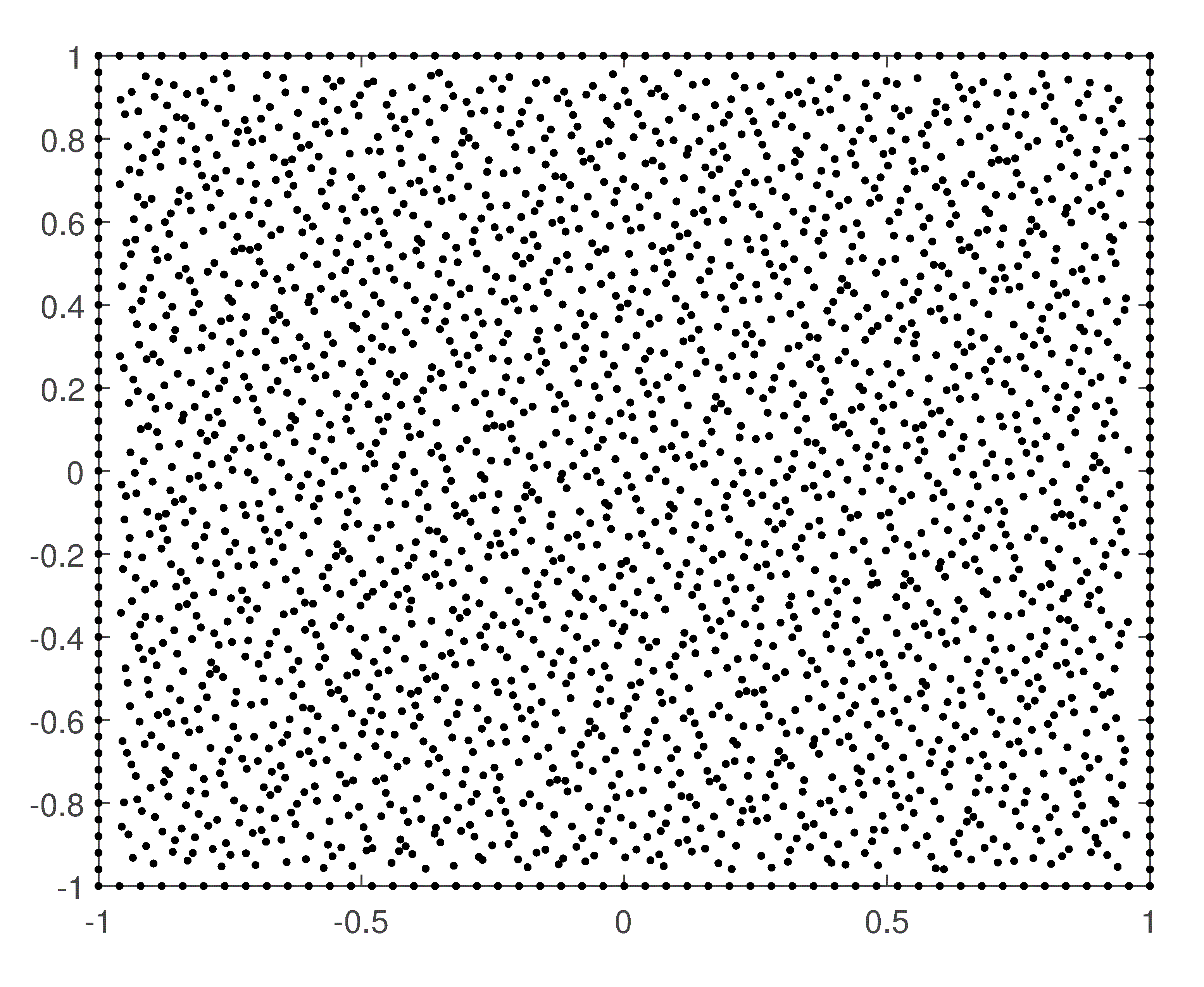
(a)

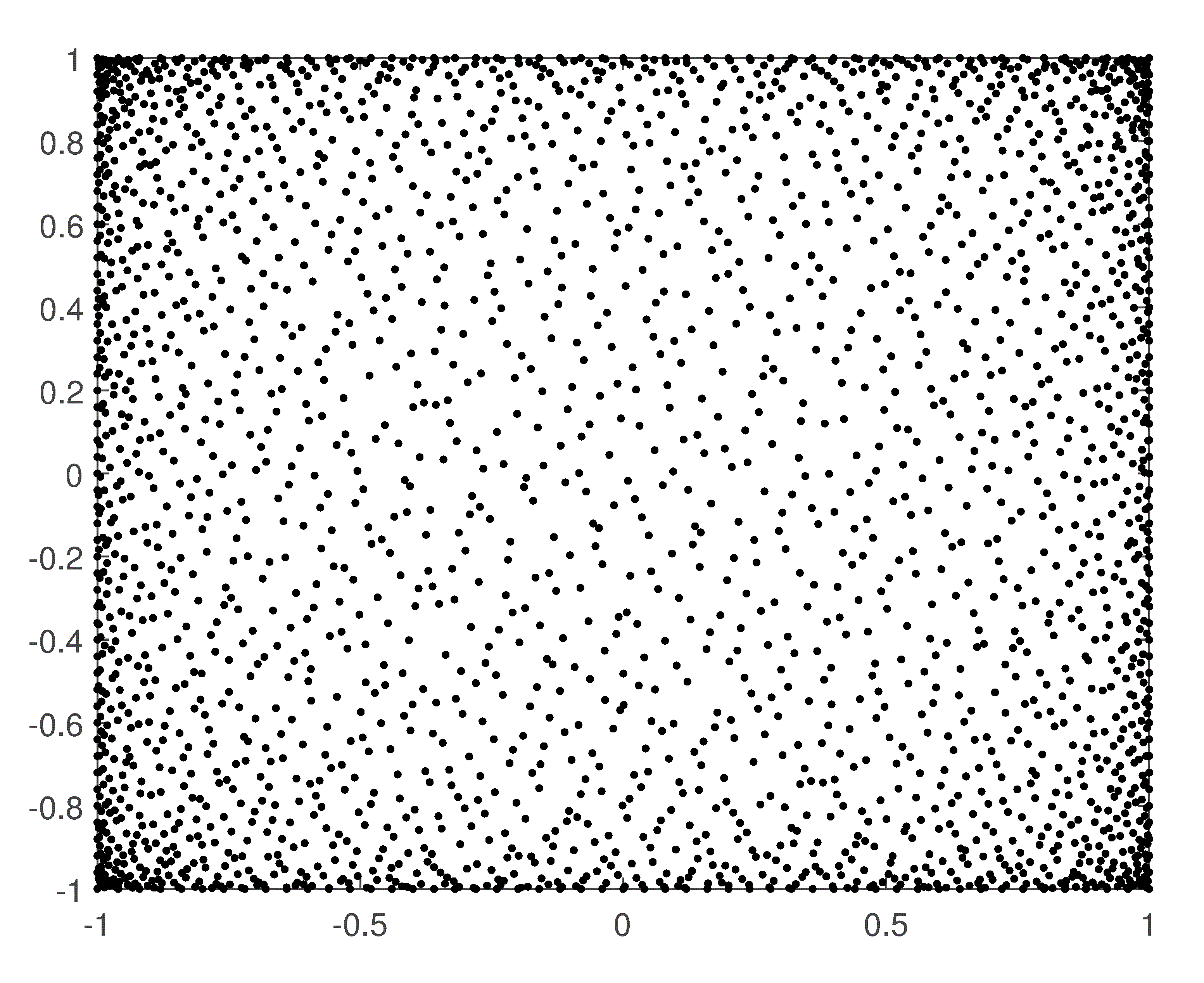
(b)

Figure 4: Example 1: in $\Omega=[-1,1]^{2}$, setting $N=2500$ (a) Halton points, and (b) nonuniform nodes with large mesh ratio by sine-transform .

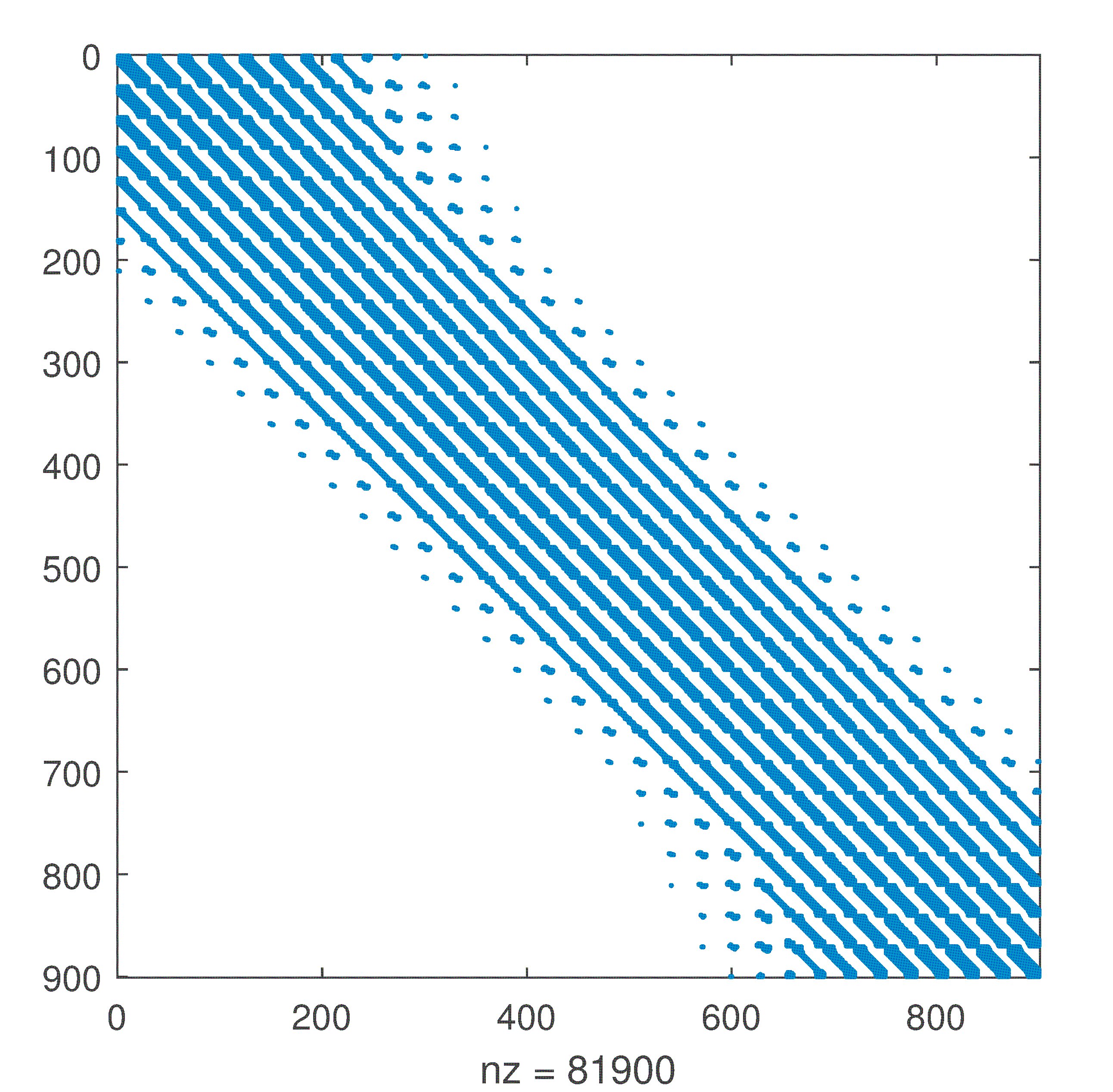
(a)

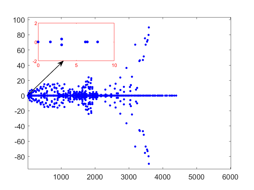
(b)

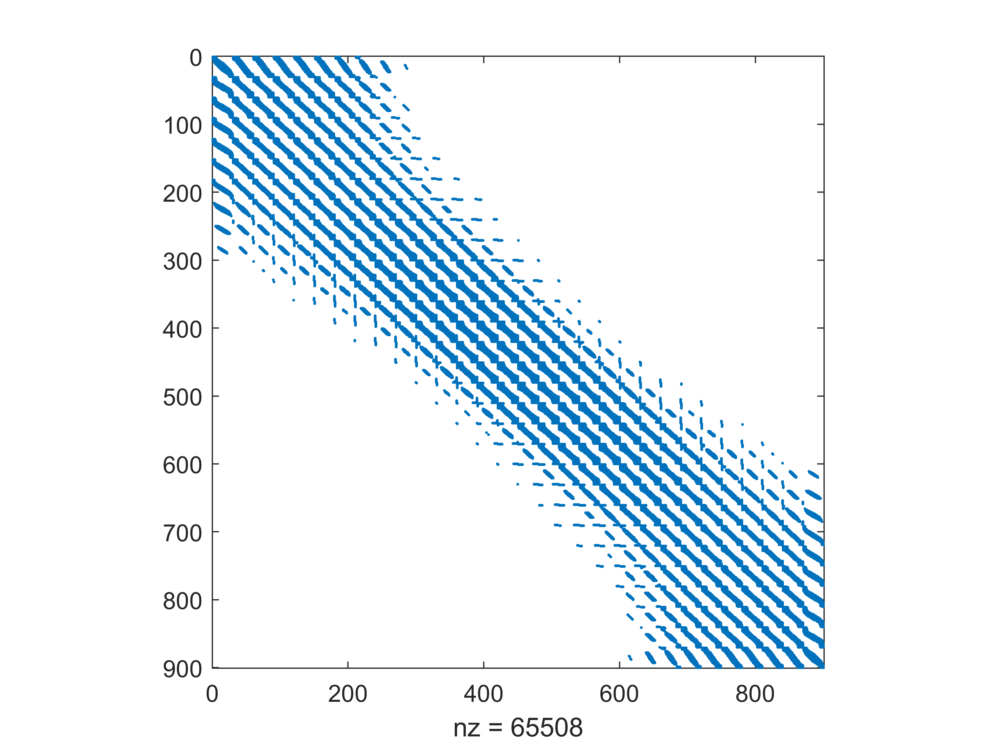
(c)

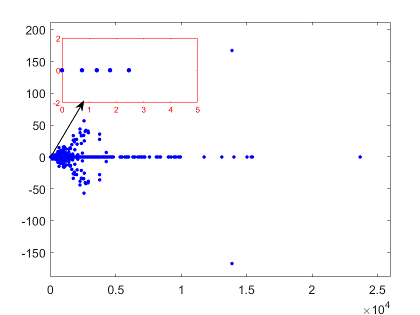
(d)

Figure 5: Example 1: results by adaptive PHS+Poly RBF-FD method for uniform and nonuniform node distribution by $N=900$, (a,c): Sparsity pattern and (b,d): eigenvalue spectra of the system matrix.

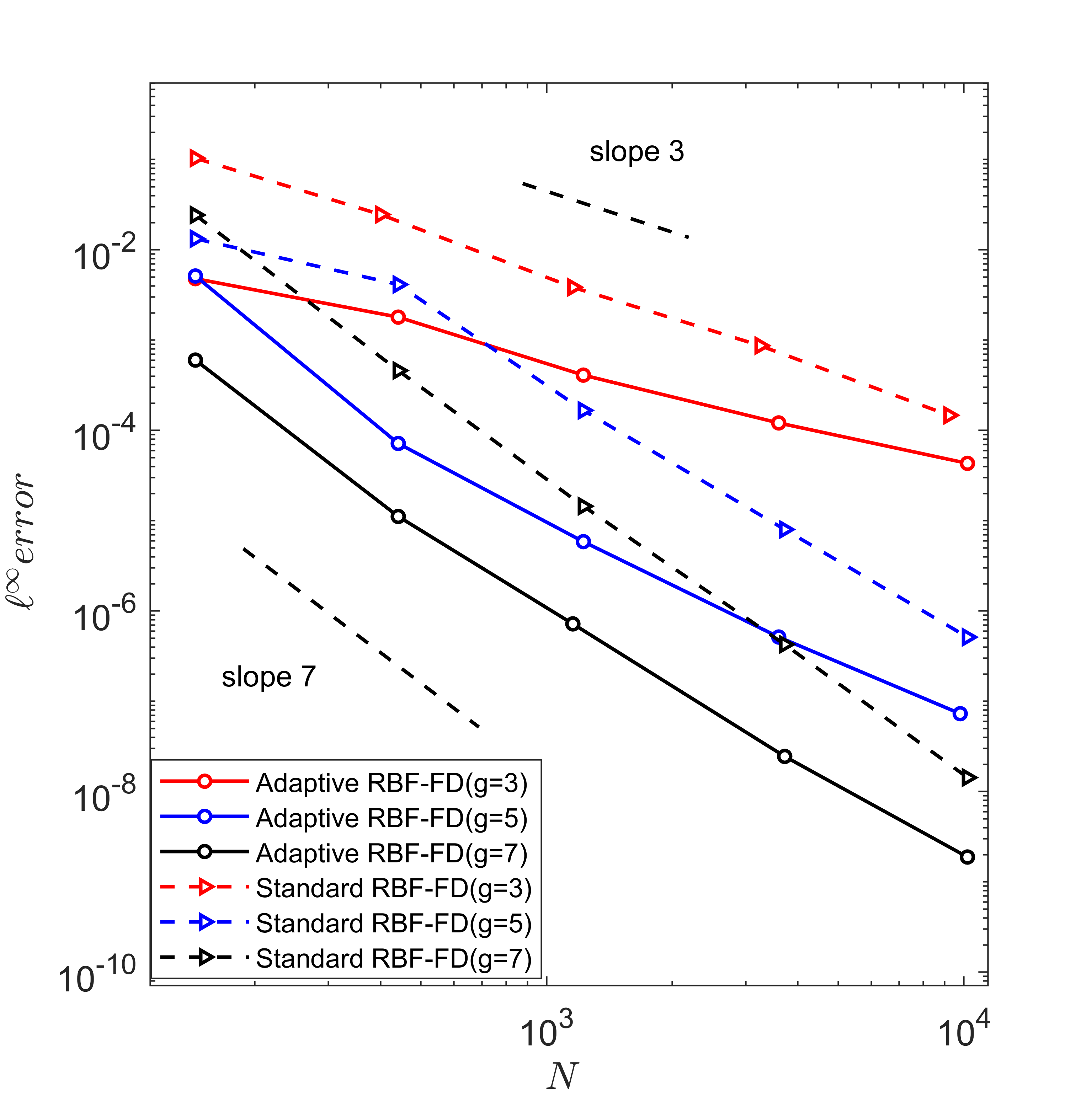
Figure 6: Example 1: convergence comparison of the adaptive PHS+Poly RBF-FD algorithm with nonuniform nodes and standard RBFFD with uniform nodes

Table 2: Example 1: the frequency of polynomial degree by the adaptive PHS+Poly RBF-FD algorithm for uniform and nonuniform node distribution in Fig. 4(b)

Polynomial degree ($p_{i}$)	5	6	7	8
Non-adaptive RBF-FD	0	0	0	6241
Proposed adaptive RBF-FD	110	1727	2694	1710

What’s more, we also extend the adaptive method to solve three dimensional problems. The Poisson equation $-\nabla^{2}u(x,y,z)=f(x,y,z)$ is solved in domain $\Omega=[-1,1]^{3}$. The exact solution is set as $u^{*}(x,y,z)=\sin\left(\pi x/2\right)\cos\left(\pi y/2\right)\cos\left(\pi z/2\right)$. The Dirichlet boundary condition is imposed on the $\partial\Omega$. Figure 7 shows interior nodes of $N=42875$ by uniform points (a) and non-uniform points (b) and (c) which generated by sine-transformation in all directions and sign-transformation $z=sign(z)*z^{2}$ along $y$ axis respectively. Figure 8 shows the convergence behavior of the RBF-FD with uniform nodes and the adaptive RBF-FD with non-uniform nodes shown in Figure 7 by setting the global order $g\in\{2,4\}$. It can be seen that both the adaptive RBF-FD and standard RBF-FD can obtain desired convergence order in 3D cases. For the global convergence rate $g=4$, Table 3 presents frequency of the three-dimensional polynomial degree $(p_{i})$ by the standard and the adaptive RBF-FD methods under two kinds of large mesh ratio node distribution respectively. It shows again that the adaptive method can have stable solutions with low computational cost by adaptively selecting the augmented polynomial basis.

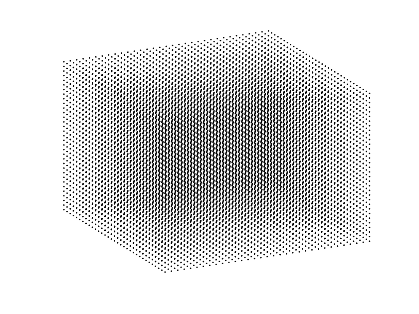
(a)

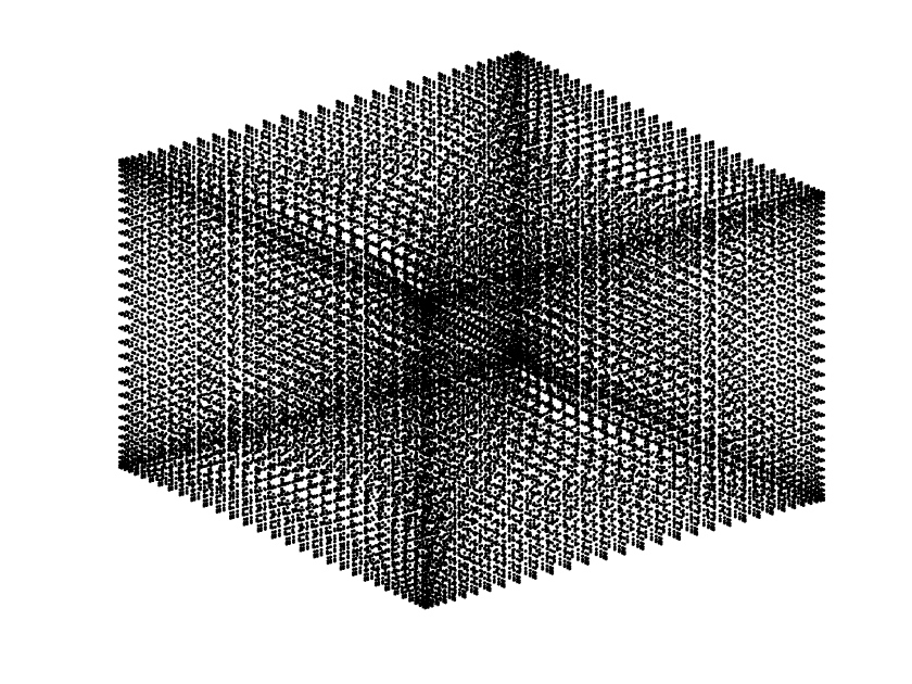
(b)

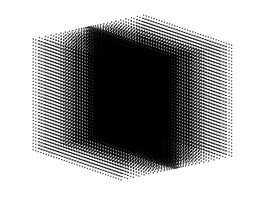
(c)

Figure 7: Example 1: For 3D case, in $\Omega=[-1,1]^{3}$ with $N=42875$ (a) uniform node distribution, (b) non-uniform distributed nodes with large mesh ratio generated by sine-transform, and (c) non-uniform nodes with large mesh ratio generated by signed-squared transform at $y$ axis.

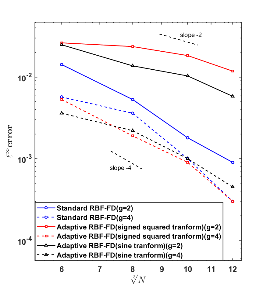
Figure 8: Example 1: For 3D case, convergence comparison of RBF-FD with uniform nodes and the adaptive RBF-FD with non-uniform nodes by $g\in\{2,4\}$.

Table 3: Example 1: For 3D case, fiixed convergence rate $g=4$ and node number $N=13824$, the frequency of polynomial degree $(p_{i})$ by the adaptive RBF-FD algorithm for uniform and non-uniform node distributions in Figure 7.

Polynomial degree ($p_{i}$)	3	4	5
RBF-FD	0	0	13824
Adaptive RBF-FD(sine transform)	800	11984	1040
Adaptive RBF-FD(signed squared transform)	0	5776	8048

4.2 Example 2: Benchmark test for adaptive FEM

This example considers a benchmark test problem from US National Institute for Standards and Technology (NIST) [20] for adaptive finite element method algorithms. It is a Poisson equation $-\Delta u(x,y)-f(x,y)=0$ in $\Omega=[0,1]^{2}$ with exact solution being an exponential peak:

$$u(x,y)=\exp\big{(}-\alpha((x-x_{0})^{2}+(y-y_{0})^{2})\big{)},$$

where $(x_{0},y_{0})$ is the peak location and $\alpha$ controls the peak strength. Dirichlet boundary conditions matching the exact solution are imposed. A typical value $\alpha=1000$ is suggested for the test. The right hand side function $f(x,y)$ satisfying the exact solution is

$$f(x,y)={-}4\left(\alpha^{2}(x-x_{0})^{2}+\alpha^{2}(y-y_{0})^{2}\right)\exp\big{(}-\alpha((x-x_{0})^{2}+(y-y_{0})^{2})\big{)}.$$

The reference solution with $\alpha=1000$ is shown in the Figure 9.

Firstly, we solve the problem with standard RBF-FD approach over quasi-uniform nodes in the domain and a fixed polynomial degree $p=6$. Figures 10 (a,b,c) show results for a quasi-uniform set of $N=2470$ nodes: nodes, numerical solution, and error function. The error is largest near the peak, indicating inaccuracy there.

We use the NodeLab algorithm NodeLab [18, 10] to generate data-dependent nodes with same number $N=2470$, which is denser in the peak zone, see Figures 10 (d). This adaptive node-distribution enhance the accuracy in the approximation. Figures 10 (e,f) show the approximated solution and point-wise absolute error with an expected global order $g=5$. Improved in accuracy around the peak zone is obvious in comparison with standard RBF-FD. By setting convergence rate $g\in\{3,5,7\}$, Figure 11 shows the $g^{th}$ convergence rate can be obtained by both method, but the proposed adaptive method are more accurate by more than one order of magnitude.

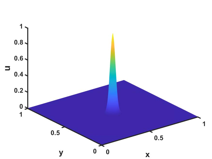
Figure 9: Example 2: A reference solution with $\alpha=1000$ and $(x_{c},y_{c})=(0.5,0.5)$

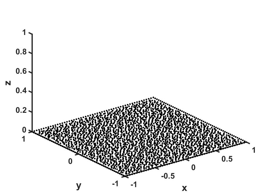
(a)

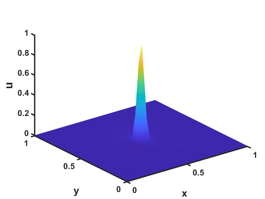
(b)

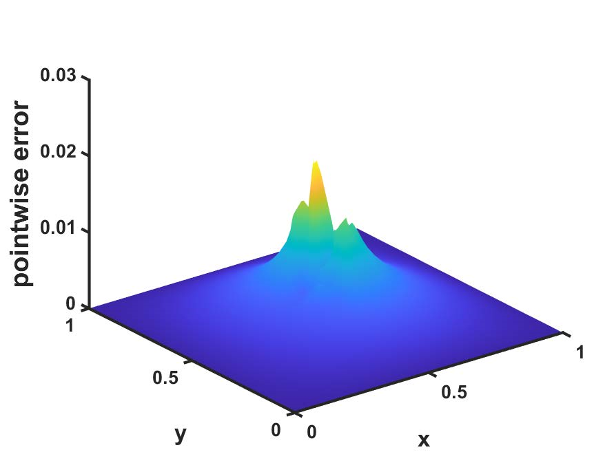
(c)

(d)

(e)

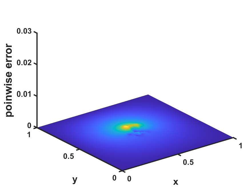
(f)

Figure 10: Example 2: setting $N=2470,\ g=5$, results by adaptive RBF-FD approach under uniform node-distribution with $p=6$ in first row and under nonuniform nodes with variable polynomial degree in second row, (a, d) node distribution, (b, e) approximated solution, and (c, f) pointwise absolute error

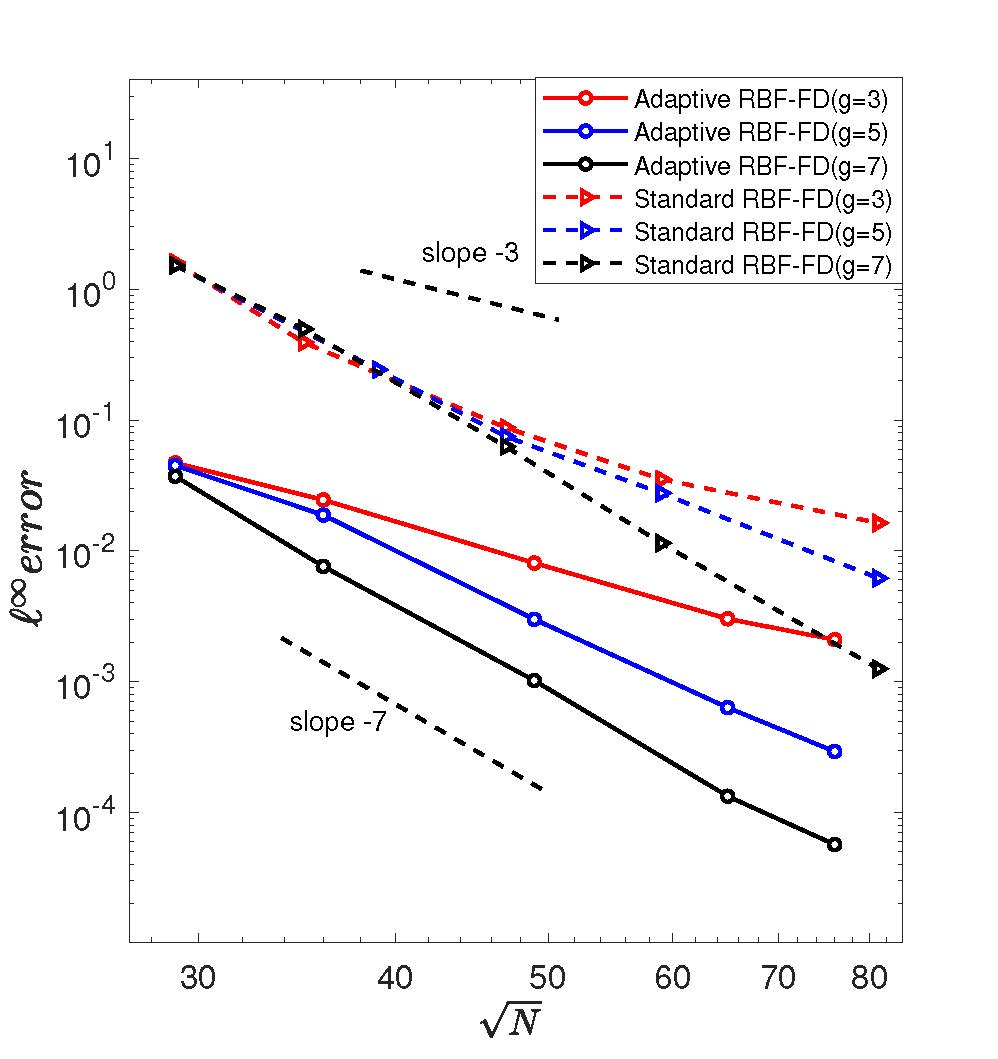
Figure 11: Example 2: Comparison of convergence of the standard RBF-FD and the Adaptive RBF-FD for a Poisson equation with delta-like exact solution.

4.3 Example 3: Solving a heat equation

We consider a time-dependent heat equation incorporated with compatible initial and boundary conditions:

$$\left\{\begin{aligned} u_{t}-\bigtriangleup u&=f(x,y,t)\qquad\ \text{for}\ (x,y,t)\in\Omega\times(0,T],\\ u(x,y,0)&=g_{1}(x,y)\quad\qquad\text{for}\ (x,y)\in\Omega,\\ u(x,y,t)&=g_{2}(x,y,t)\qquad\ \text{for}\ (x,y,t)\in\partial\Omega\times(0,T].\end{aligned}\right.$$

in $\Omega=[-1,1]^{2}$ with exact solution $u^{*}(x,y,t)=\exp(t)\cos(\pi x)\cos(\pi y)$. The initial condition and boundary conditions are generated from the exact solution:

$$g_{1}(x,y)=\cos(\pi x)\cos(\pi y),\qquad g_{2}(x,y,t)=\exp(t)\cos(\pi x)\cos(\pi y),$$

and so as the source term $f(x,y,t)=(1+2\pi^{2})u^{*}(x,y,t)$.

We discretize the PDE (4.3) in time using the $\theta$-method over $M$ time steps with step size $\tau=T/M$:

$$\begin{split}\frac{u^{n}-u^{n-1}}{\tau}=\theta(\bigtriangleup u^{n}+f^{n})+(1-\theta)(\bigtriangleup u^{n-1}+f^{n-1}).\end{split}$$

We consider both the backward-Euler scheme with $\theta=1$:

$$\begin{split}u^{n}-\tau\bigtriangleup u^{n}&=u^{n-1}+\tau f^{n}(x,y,t),\end{split}$$

and Crank-Nicolson scheme with $\theta=1/2$:

$$\begin{split}u^{n}-\frac{\tau}{2}\bigtriangleup u^{n}&=u^{n-1}+\frac{\tau}{2}\bigtriangleup u^{n-1}+\frac{\tau}{2}\bigtriangleup(f^{n}+f^{n-1}).\end{split}$$

The nonuniform discrete points in the domain is generated by the same method as described in Example 1. The user-defined global convergence rate set to $g=\{3,5,7\}$ and PHS kernel is $\phi(r)=r^{2m-1},m=3$. Figure 12 illustrate the convergence behavior of the solutions by the $\ell^{\infty}(\Omega,T)$ error. Figure 12 (a) plots the space convergence results with respect to $\sqrt{N}$ by $\tau=1E-7,T=1E-6$, discrete points in domain nodes $N\in[10^{2},70^{2}]$. The local stencil is set as $n_{s}=100$. The result shows that the convergence rate $g$ is obtained. Figure 12 (b) illustrates the time convergence results by $T=1$, $N=64^{2}$. It can be observed that the Crank-Nicolson method achieves second-order accuracy in time, while the backward-Euler method achieves first-order accuracy in time. These results suggest that the proposed adaptivity does not cause instability when solving parabolic equations.

\begin{overpic}[height=156.49014pt]{FIG1new//q3_convergence_NE.png} \put(47.0,90.0){\small$(a)$} \end{overpic}

\begin{overpic}[height=156.49014pt]{FIG1new//q3t_convergence.png} \put(45.0,94.0){\small$(b)$} \end{overpic}

Figure 12: Example 3: the convergence results of adaptive RBFFD (PHS+Poly) for solving the heat equation (4.3): (a) space convergence by $\tau=1E-7,T=1E-6,\ N\in[10^{2},70^{2}]$; (b) time convergence by $\tau\in[0.02,0.2]$, $T=1$, $N=64^{2}$

4.4 Example 4: Application in elastic wave model

We apply the adaptive RBF-FD method to the following elastic wave Navier equation [31]:

$$\left\{\begin{array}[]{l}\mu\Delta u_{1}+(\lambda+\mu)({\partial_{x}^{2}u_{1}}+{\partial_{x}\partial_{y}u_{2}})+\omega^{2}\rho u_{1}=f_{1}\\ \mu\Delta u_{2}+(\lambda+\mu)({\partial_{x}\partial_{y}u_{1}}+{{\partial_{y}^{2}}u_{2}})+\omega^{2}\rho u_{2}=f_{2}\\ \end{array},\right.$$ (11)

with $\omega$ being the angular frequency and $\lambda,\ \mu$ being Lamé constants. We assume the medium is homogeneous and set the density $\rho\equiv 1$ after normalization. The time-harmonic displacement vector $\bm{u}=(u_{1},u_{2})^{T}$ satisfies the lowest-order absorbing boundary condition:

$$\mathbf{T}^{(\mathbf{n})}(\bm{u})-i\eta\bm{u}=\mathbf{g}\quad\text{ on }\ \gamma=\partial\Omega,$$

where the traction operator $\mathbf{T}^{(\bm{n})}$ is

$$\mathbf{T}^{(\bm{n})}(\bm{u})=2\mu\frac{\partial\bm{u}}{\partial\bm{n}}+\lambda\bm{n}\nabla\cdot\bm{u}+\mu\bm{n}\times(\nabla\times\bm{u}),$$

with $\bm{n}$ being the unit normal vector and a real-valued matrix function $\eta$ is defined by

$$\eta=\omega\rho\left(C_{\mathrm{P}}\bm{n}\bm{n}^{T}+C_{\mathrm{S}}\bm{s}\bm{s}^{T}\right),C_{\mathrm{P}}=\sqrt{\frac{\lambda+2\mu}{\rho}},\ C_{\mathrm{S}}=\sqrt{\frac{\mu}{\rho}}$$

with $\bm{s}$ being a unit tangent vector. We study the problem in $\Omega=[0,1]^{2}$, and nonuniform distribution nodes are obtained by using the transformation $z=(\sin(\pi z)+1)/2$ on each coordinate. The components of the exact displacement field $\mathbf{u}=(u_{1},u_{2})^{T}$ is given as follows

$$\left\{\begin{array}[]{l}\displaystyle u_{1}=\alpha_{\mathrm{S}}\left\{\exp(-\alpha_{\mathrm{S}}y)-\frac{2\kappa_{R}^{2}}{\kappa_{R}^{2}+\alpha_{\mathrm{S}}^{2}}\exp(-\alpha_{\mathrm{P}}y)\right\}\exp(i\kappa_{R}x)\\ \displaystyle u_{2}=i\kappa_{R}\left\{\exp(-\alpha_{\mathrm{S}}y)-\frac{2\alpha_{\mathrm{P}}\alpha_{\mathrm{S}}}{\kappa_{R}^{2}+\alpha_{\mathrm{S}}^{2}}\exp(-\alpha_{\mathrm{P}}y)\right\}\exp(i\kappa_{R}x)\end{array},\right.$$ (12)

where $\alpha_{\mathrm{P}}=\sqrt{\kappa_{R}^{2}-\kappa_{\mathrm{P}}^{2}},\ \alpha_{\mathrm{S}}=\sqrt{\kappa_{R}^{2}-\kappa_{S}^{2}}$. We take the Lamé constants $\lambda=2$, $\mu=1$, angular frequency $\omega=2\pi$, which decide the value of $\kappa_{R}=2.14\pi,\ \kappa_{P}=\pi,\ \kappa_{S}=2\pi$. We report the relative $L^{2}$-error:

$$E_{\eta}=\frac{\left\|\bm{u}^{e}-\bm{u}^{n}\right\|_{2}}{\left\|\bm{u}^{e}\right\|_{2}}=\left({\frac{\int_{\Omega}\left(\overline{\bm{u}}^{e}-\overline{\bm{u}}^{n}\right)^{T}\left(\bm{u}^{e}-\bm{u}^{n}\right)d\Omega}{\int_{\Omega}\left(\overline{\bm{u}}^{e}\right)^{T}\left(\bm{u}^{e}\right)d\Omega}}\right)^{1/2}.$$

Setting the global convergence order $g\in\{3,5,7\}$, Figure 13 (a) compares the proposed adaptive PHS+Poly RBF-FD on nonuniform nodes and standard RBF-FD on uniform nodes. The adaptive method achieves higher accuracy while maintaining the desired convergence rate.

Angular frequency $\omega$ determines oscillatory behavior: higher $\omega$ causes more frequent oscillations. Figure 13 (b) plots error $E_{\eta}$ versus $\omega$ for $g=5$. Errors progressively worsen with increasing $\omega$, but the adaptive RBF-FD is less sensitive. Figure 14 plots the real and imaginary parts of $u_{1}$,$u_{2}$ at circle $r=0.5$ for $N=3600$. Both methods recover the analytic solutions well. For $g=5$, standard RBF-FD has $8.2\times 10^{5}$ nonzeros while adaptive RBF-FD has $6.5\times 10^{5}$, a reduction of $1.7\times 10^{5}$ nonzeros. For $g=7$, adaptive RBF-FD reduces nonzeros by $2.3\times 10^{5}$. The adaptive method saves more computation cost at higher accuracy. For realistic elastic wave problems, the adaptive RBF-FD could be an efficient alternative for practitioners.

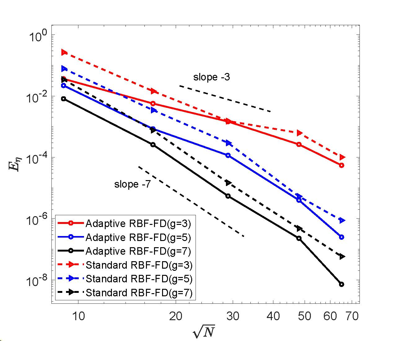
(a)

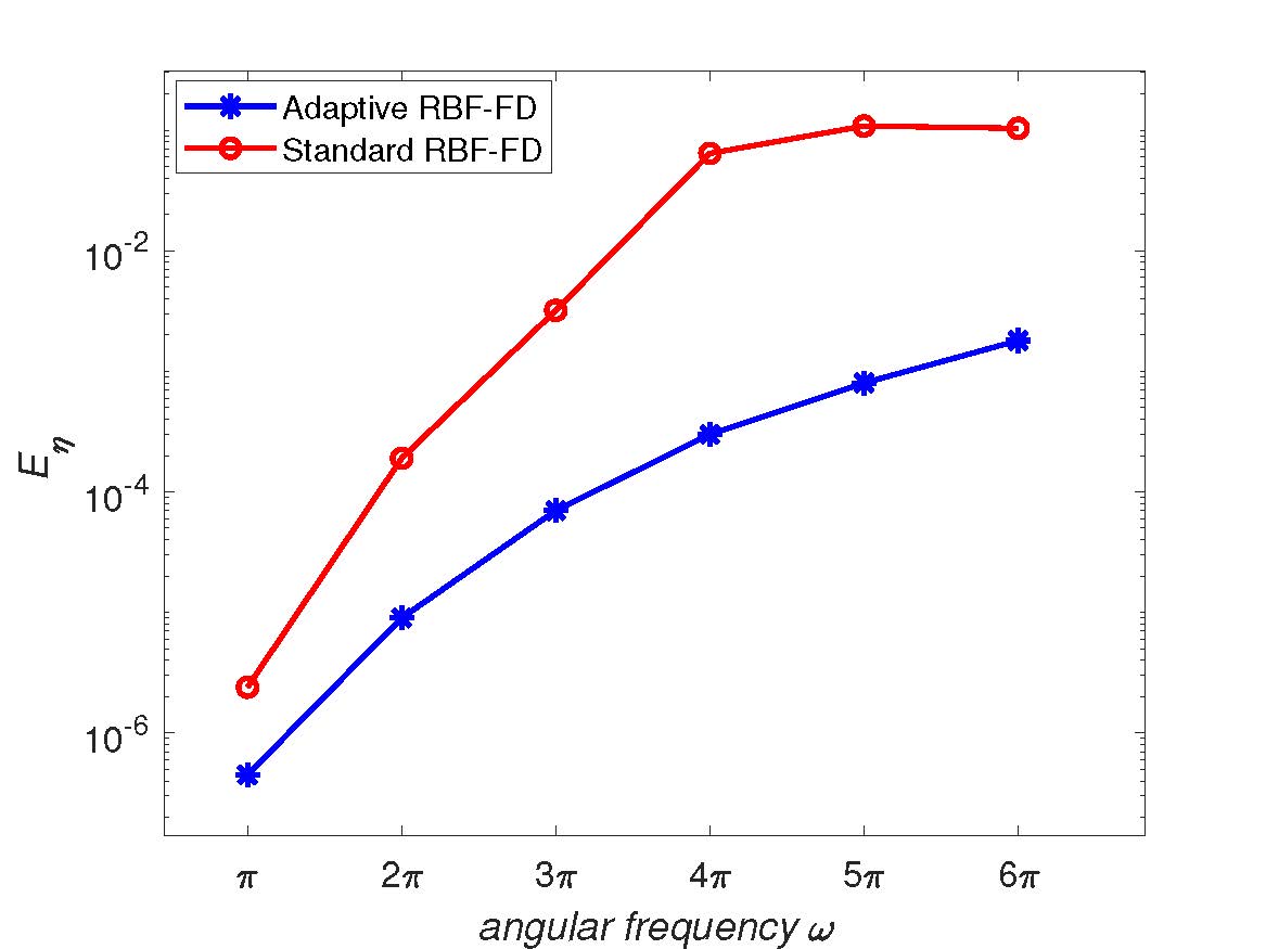
(b)

Figure 13: Example 4: (a) Comparison of convergence of the standard RBF-FD and the Adaptive RBF-FD for Navier equation. (b) The relative errors with respect the angular frequencies.

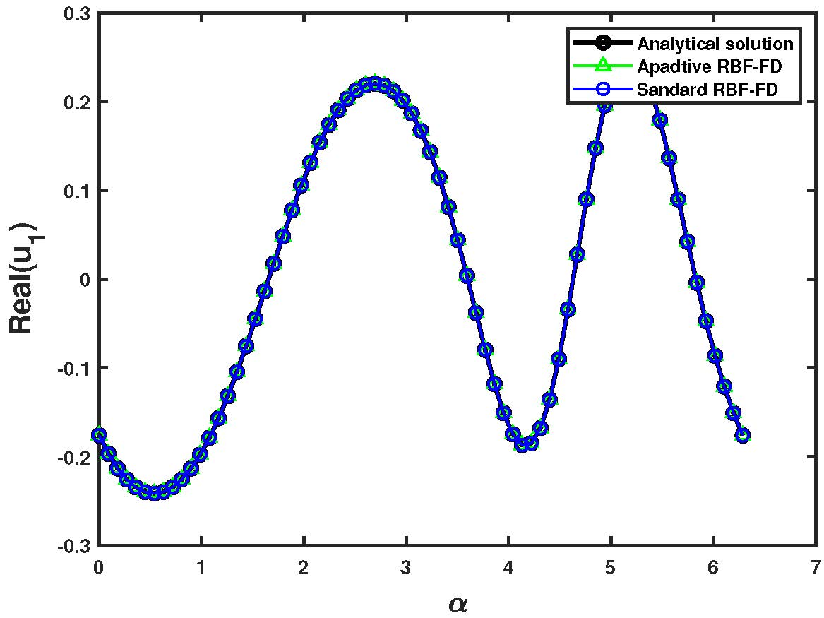
(a)

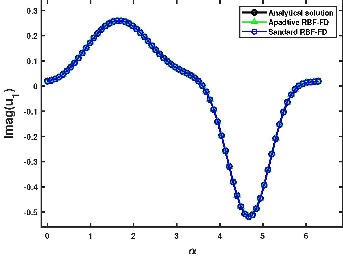
(b)

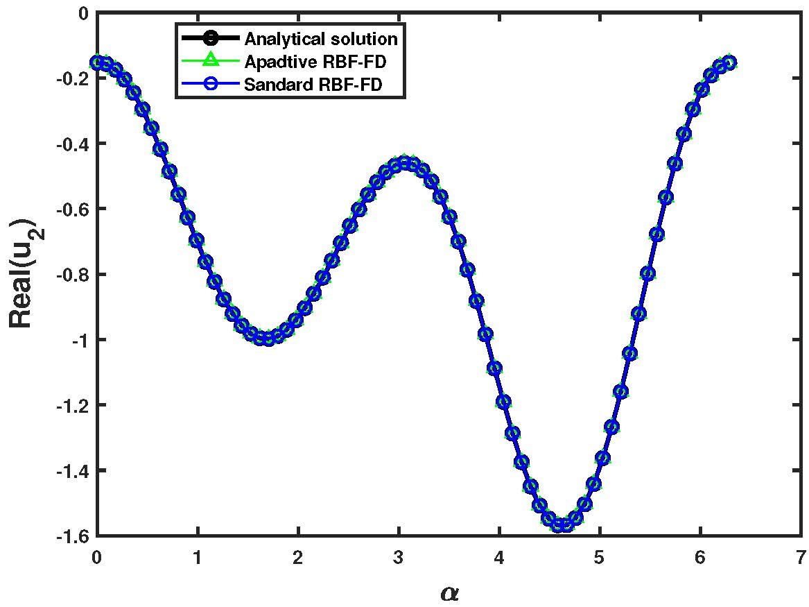
(c)

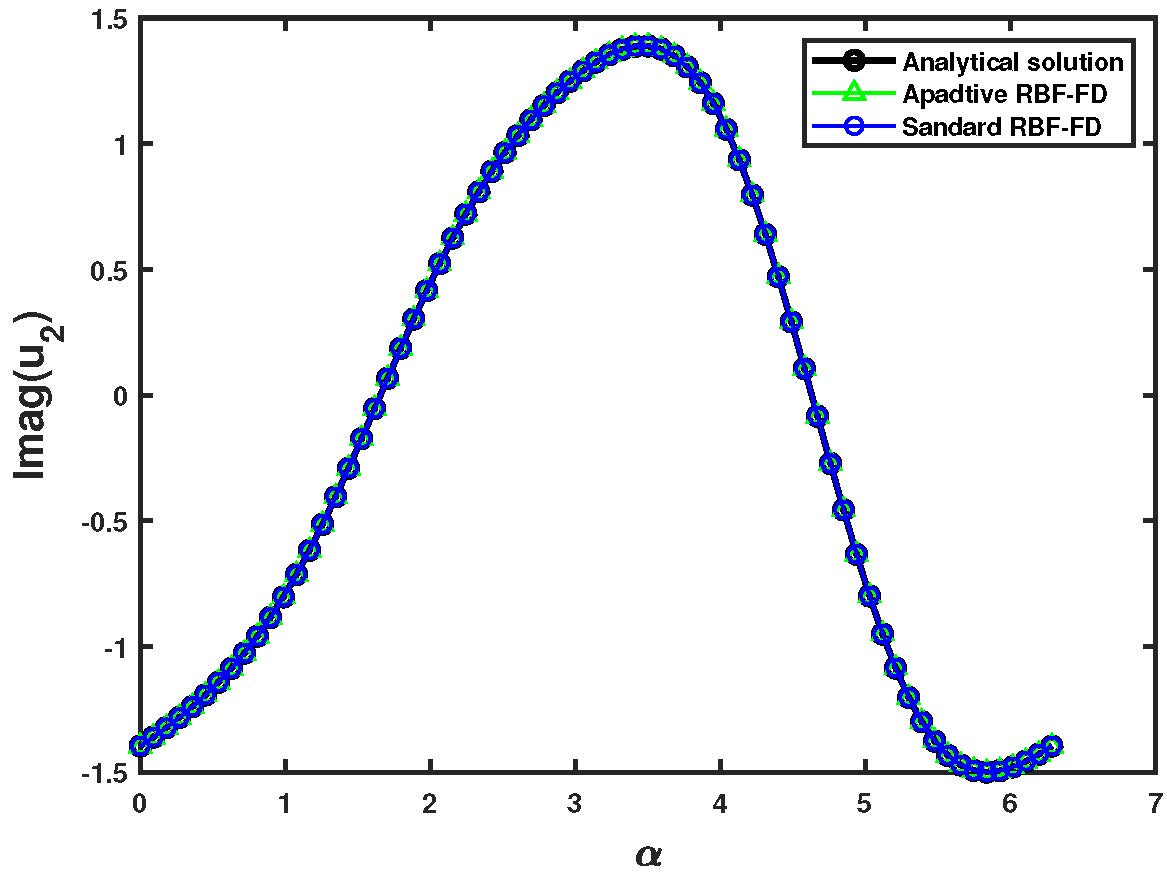
(d)

Figure 14: Example 4: results by adaptive RBF-FD for the Navier equation with $\omega=2\pi$ and $N=3600$.

5 Conclusions

We developed an adaptive PHS+Poly RBF-FD method well suited for high-order approximations over nonuniform nodes. For uniform nodes, adaptive RBF-FD simplifies to standard RBF-FD. By varying the polynomial degree at each point based on the desired global convergence order, we constructed the adaptive scheme. Our adaptive method provides several advantages: it achieves the specified global convergence order and high accuracy for nonuniform nodes while performing comparably to standard RBF-FD for uniform nodes. The differentiation matrix is sparser, suggesting lower computational cost that will increase for large-scale problems solved using sparse linear solvers. By adaptively choosing local stencil sizes and polynomial degrees based on node density, the proposed method saves the computational resources by balancing accuracy and efficiency. In other words, the proposed method is not aimed to improve accuracy. The method also applies to both steady and time-dependent problems, as demonstrated for the heat equation and elastic wave problems. These characteristics make the adaptive RBF-FD method a powerful tool for solving PDEs using scattered data. Future work will explore applications to large-scale and 3D problems to fully leverage the computational efficiency gains of the adaptive method.

References

- [1] V. Bayona, N. Flyer, and B. Fornberg, On the role of polynomials in RBF-FD approximations: III. behavior near domain boundaries, Journal of Computational Physics, (2019).
- [2] V. Bayona, N. Flyer, B. Fornberg, and G. A. Barnett, On the role of polynomials in RBF-FD approximations: II. numerical solution of elliptic PDEs, Journal of Computational Physics, 332 (2017), pp. 257–273.
- [3] V. Bayona, M. Moscoso, M. Carretero, and M. Kindelan, RBF-FD formulas and convergence properties, Journal of Computational Physics, 229 (2010), pp. 8281–8295.
- [4] G. Chandhini and Y. Sanyasiraju, Local RBF-FD solutions for steady convection–diffusion problems, International Journal for Numerical Methods in Engineering, 72 (2007), pp. 352–378.
- [5] B. arler, A radial basis function collocation approach in computational fluid dynamics, Cmes-computer Modeling in Engineering & Sciences, 7 (2005), pp. 185–194.
- [6] B. arler and R. Vertink, Meshfree explicit local radial basis function collocation method for diffusion problems, Computers & Mathematics with Applications, 51 (2006), pp. 1269–1282.
- [7] P. P. Chinchapatnam, K. Djidjeli, P. Nair, and M. Tan, A compact RBF-FD based meshless method for the incompressible Navier Stokes equations, Proceedings of the Institution of Mechanical Engineers, Part M: Journal of Engineering for the Maritime Environment, 223 (2009), pp. 275–290.
- [8] N. Flyer, B. Fornberg, V. Bayona, and G. A. Barnett, On the role of polynomials in RBF-FD approximations: I. interpolation and accuracy, Journal of Computational Physics, 321 (2016), pp. 21–38.
- [9] N. Flyer, E. Lehto, S. Blaise, G. B. Wright, and A. St-Cyr, A guide to RBF-generated finite differences for nonlinear transport: Shallow water simulations on a sphere, Journal of Computational Physics, 231 (2012), pp. 4078–4095.
- [10] B. FORNBERG and N. FLYER, Fast generation of 2-D node distributions for mesh-free PDE discretizations, Computers & Mathematics with Applications, 69 (2015), pp. 531–544.
- [11] B. Fornberg and N. Flyer, Solving PDEs with radial basis functions, Acta Numerica, 24 (2015), pp. 215–258.
- [12] B. Fornberg and E. Lehto, Stabilization of RBF-generated finite difference methods for convective PDEs, Journal of Computational Physics, 230 (2011), pp. 2270–2285.
- [13] M. Kindelan, D. Álvarez, and P. Gonzalez-Rodriguez, Frequency optimized RBF-FD for wave equations, Journal of Computational Physics, (2018).
- [14] B. Martin, A. Elsherbeni, G. E. Fasshauer, and M. Hadi, Improved FDTD method around dielectric and PEC interfaces using RBF-FD techniques, in Applied Computational Electromagnetics Society Symposium (ACES), 2018 International, IEEE, 2018, pp. 1–2.
- [15] B. Martin and B. Fornberg, Using radial basis function-generated finite differences (RBF-FD) to solve heat transfer equilibrium problems in domains with interfaces, Engineering Analysis with Boundary Elements, 79 (2017), pp. 38–48.
- [16] B. Martin, B. Fornberg, and A. St-Cyr, Seismic modeling with radial-basis-function-generated finite differences, Geophysics, 80 (2015), pp. T137–T146.
- [17] P. Mishra, S. Nath, G. Fasshauer, and M. Sen, Frequency-domain meshless solver for acoustic wave equation using a stable radial basis-finite difference (RBF-FD) algorithm with hybrid kernels, in SEG Technical Program Expanded Abstracts 2017, Society of Exploration Geophysicists, 2017, pp. 4022–4027.
- [18] P. K. Mishra, NodeLab— a matlab package for meshfree node-generation and adaptive refinement, (2019). https://github.com/pankajkmishra/NodeLab.
- [19] P. K. Mishra, G. E. Fasshauer, M. K. Sen, and L. Ling, A stabilized radial basis-finite difference (RBF-FD) method with hybrid kernels, Computers & Mathematics with Applications, (2018).
- [20] W. F. Mitchell, A collection of 2D elliptic problems for testing adaptive grid refinement algorithms, Applied mathematics and computation, 220 (2013), pp. 350–364.
- [21] A. Petras, L. Ling, and S. J. Ruuth, An RBF-FD closest point method for solving PDEs on surfaces, Journal of Computational Physics, 370 (2018), pp. 43–57.
- [22] L. Santos, N. Manzanares-Filho, G. Menon, and E. Abreu, Comparing RBF-FD approximations based on stabilized Gaussians and on polyharmonic splines with polynomials, International Journal for Numerical Methods in Engineering, (2017).
- [23] R. Schaback, A computational tool for comparing all linear PDE solvers, Advances in Computational Mathematics, 41 (2014), pp. 333–355.
- [24] , Error Analysis of Nodal Meshless Methods, Springer International Publishing, 04 2017, pp. 117–143.
- [25] V. Shankar, The overlapped radial basis function-finite difference (RBF-FD) method: A generalization of RBF-FD, Journal of Computational Physics, 342 (2017), pp. 211–228.
- [26] V. Shankar, G. B. Wright, R. M. Kirby, and A. L. Fogelson, A radial basis function (RBF)-finite difference (FD) method for diffusion and reaction–diffusion equations on surfaces, Journal of scientific computing, 63 (2015), pp. 745–768.
- [27] J. Slak and G. Kosec, Refined RBF-FD solution of linear elasticity problem, in 2018 3rd International Conference on Smart and Sustainable Technologies (SpliTech), IEEE, 2018, pp. 1–6.
- [28] A. Tolstykh and D. Shirobokov, On using radial basis functions in a “finite difference mode” with applications to elasticity problems, Computational Mechanics, 33 (2003), pp. 68–79.
- [29] G. B. Wright, Radial basis function interpolation: numerical and analytical developments, PhD thesis, University of Colorado at Boulder, 2003.
- [30] G. B. Wright and B. Fornberg, Scattered node compact finite difference-type formulas generated from radial basis functions, Journal of Computational Physics, 212 (2006), pp. 99–123.
- [31] L. Yuan and Y. Liu, A Trefftz-discontinuous Galerkin method for time-harmonic elastic wave problems, Computational and Applied Mathematics, 38 (2019), pp. 1–29.
- [32] S. Zhang, Meshless symplectic and multi-symplectic local RBF collocation methods for Hamiltonian PDEs, Journal of Scientific Computing, 88 (2021), p. 90.