Average Treatment Effect Estimation in Observational Studies with Functional Covariates

Abstract

Functional data analysis is an important area in modern statistics and has been successfully applied in many fields. Although many scientific studies aim to find causations, a predominant majority of functional data analysis approaches can only reveal correlations. In this paper, average treatment effect estimation is studied for observational data with functional covariates. This paper generalizes various state-of-art propensity score estimation methods for multivariate data to functional data. The resulting average treatment effect estimators via propensity score weighting are numerically evaluated by a simulation study and applied to a real-world dataset to study the causal effect of duloxitine on the pain relief of chronic knee osteoarthritis patients.

Keywords: Functional principal component analysis; Functional regression; Direct modeling; Covariate balancing; Magnetic resonance imaging.

1 Introduction

Functional data analysis (FDA) has become increasingly important in modern statistics and has been successfully applied in a variety of scientific fields. Apart from books on general introductions to FDA (e.g., Bosq, 2000; Ramsay and Silverman, 2005; Ferraty and Vieu, 2006; Horváth and Kokoszka, 2012; Hsing and Eubank, 2015; Kokoszka and Reimherr, 2017), recent advances of FDA, including innovative methodologies, profound theories, efficient algorithms, and successful applications, have been illustrated by numerous survey papers (e.g., Guo, 2004; Müller, 2008; Delicado et al., 2010; Geenens, 2011; Hörmann and Kokoszka, 2012; Cuevas, 2014; Marron and Alonso, 2014; Shang, 2014; Wang et al., 2016; Chen et al., 2017; Nagy, 2017; Vieu, 2018; Kokoszka and Reimherr, 2019).

A majority of FDA methods can only reveal correlations primarily via either functional regression models (for reviews see e.g., Morris, 2015; Greven and Scheipl, 2017; Paganoni and Sangalli, 2017; Reiss et al., 2017) or correlation measures (e.g., Leurgans et al., 1993; Dubin and Müller, 2005; Cupidon et al., 2008; Eubank and Hsing, 2008; Lian, 2014; Shin and Lee, 2015; Zhou et al., 2018). However, FDA methods for causal inference is underdeveloped despite the importance of causation in many scientific studies. Among very few exceptions, almost all of them focus on randomized clinical trials (e.g., Lindquist, 2012; McKeague and Qian, 2014; Ciarleglio et al., 2015, 2018; Zhao et al., 2018; Zhao and Luo, 2019). In classical causal inference for observational studies where multivariate data are of primary interest, the propensity score (Rosenbaum and Rubin, 1983) plays an important role and has been widely applied in epidemiology and political science among others. Despite its popularity, its use in FDA to study causations in observational studies is nearly void.

The main contribution of this paper is to introduce and adapt various state-of-art propensity score methods to observational functional data. We consider the scenario where the treatment is binary and at least one covariate is functional. We generalize the definition of the propensity score to functional data, and study two types of propensity score estimations. The propensity score is estimated by either directly fitting a functional regression model or balancing appropriate functions of the covariates. This paper in particular focuses on propensity score weighting (e.g., Rosenbaum, 1987; Robins et al., 2000; Hirano et al., 2003), although the propensity score may be used to adjust for confounding through other means, e.g., matching (e.g., Rosenbaum and Rubin, 1985; Rosenbaum, 1989; Abadie and Imbens, 2006) and subclassification (e.g., Rosenbaum and Rubin, 1984; Rosenbaum, 1991; Hansen, 2004). A systematic comparison of two popular propensity-score-weighted average treatment effect estimators is provided in both a simulation study and a real data application.

The rest of the paper proceeds as follows. Section 2 provides the problem setup and generalizes the classical definition of the propensity score to functional data where the treatment is binary and one covariate is functional. Section 3 introduces two types of propensity score estimations via direct modeling and covariate balancing respectively and two widely used average treatment effect estimators via propensity score weighting. The two average treatment effect estimators based on a variety of estimated propensity score weights are comprehensively compared in a simulation study in Section 4. They are also applied in a real data analysis in Section 5 to study the causal effect of duloxitine on the pain relief of chronic knee osteoarthritis patients. Discussion in Section 6 concludes the paper.

2 Framework

Suppose that $Y$ is a continuous outcome, $T$ is a binary treatment variable which equals either $0$ (control) or $1$ (treatment), ${\bf W}$ is a multivariate covariate, and $X(\cdot)$ is a functional covariate defined on a compact domain $\mathcal{T}$. Suppose that $E\int_{\mathcal{T}}\{X(t)\}^{2}\,dt<\infty$ and $X(\cdot)$ is smooth, e.g., continuous or twice-differentiable. Without loss of generality $E({\bf W})={\bf 0}$, $\mathcal{T}=[0,1]$ and $E\{X(t)\}=0$ for all $t\in[0,1]$.

Let $Y(1)$ and $Y(0)$ represent the potential values of $Y$ when $T=1$ and $0$ respectively. In practice $Y=TY(1)+(1-T)Y(0)$ is observable but $Y(1)$ and $Y(0)$ are not both observable. Based on $\{(Y_{i},T_{i},{\bf W}_{i},\{X_{i}(t):t\in[0,1]\}):i=1,\ldots,n\}$, which are independently and identically distributed (i.i.d.) copies of $(Y,T,{\bf W},\{X(t):t\in[0,1]\})$, we aim to estimate the average treatment effect $\tau=E\{Y(1)-Y(0)\}$.

We assume that each $X_{i}(\cdot)$ is fully observed, but the methods below are also applicable for densely measured $X_{i}(\cdot)$ since its entire trajectory can be accurately recovered by smoothing (e.g., Zhang and Chen, 2007). In this paper we only consider low-dimensional ${\bf W}_{i}$. The handling of high-dimensional multivariate covariates is beyond the scope of this paper but is a promising topic for future research (e.g., Belloni et al., 2014; Farrell, 2015; Belloni et al., 2017; Chernozhukov et al., 2018; Ning et al., 2018).

Similar to its classical counterpart (e.g., Rosenbaum and Rubin, 1983; Robins et al., 2000), the propensity score is defined by

$$p({\bf W}_{i},X_{i})=P(T_{i}=1\mid{\bf W}_{i},X_{i}(\cdot)).$$ (1)

In this paper we make the following two assumptions:

Assumption 1.

$$T_{i}\perp\left(Y_{i}(0),Y_{i}(1)\right)\mid\left({\bf W}_{i},X_{i}(\cdot)\right),$$

where “$\perp$” represents independence.

Assumption 2.

The propensity score satisfies

$$0<P(T_{i}=1\mid{\bf W}_{i}={\bf w},X_{i}(\cdot)=x(\cdot))<1,$$

for all vectors ${\bf w}$ and all functions $x(\cdot)$ defined on $[0,1]$ such that $\int_{0}^{1}\{x(t)\}^{2}\,dt<\infty$ .

Assumptions 1 and 2 are straightforward generalizations of the commonly used strong ignorability and positivity assumptions in classical causal inference respectively. Assumption 1 implies that there is no unmeasured covariate, while Assumption 2 essentially requires that every sample has a positive probability of receiving the treatment or being in the control group.

3 Methodology

In this section, we introduce various methods for propensity score estimation and two average treatment effect estimators via propensity score weighting.

3.1 Propensity Score Estimation

We propose two types of propensity score estimations, one via direct modeling and the other via covariate balancing. They will be introduced in Sections 3.1.1 and 3.1.2 respectively.

3.1.1 Direct Modeling

To estimate the propensity score $p({\bf W}_{i},X_{i})$, one may assume a parametric model for $p({\bf W}_{i},X_{i})$ and fit it with an appropriate estimation procedure.

The simplest model might be the generalized functional partial linear model (GFPLM):

$$\text{logit}\left\{p({\bf W}_{i},X_{i})\right\}=\alpha_{0}+\mbox{\boldmath$\alpha$}_{1}^{\top}{\bf W}_{i}+\int_{0}^{1}\beta(t)X_{i}(t)\,dt,$$ (2)

where $\text{logit}(x)=\log\{x/(1-x)\}$ and the scalar $\alpha_{0}$, vector $\mbox{\boldmath$\alpha$}_{1}$ and function $\beta(\cdot)$ are unknown parameters to be estimated. Apparently the GFPLM is an extension of James (2002), Müller and Stadtmüller (2005) and Shin (2009).

Similar to fitting other functional regression models considered in the FDA literature, regularization for the functional coefficient $\beta$ is needed to fit (2). Popular regularizations include the truncated basis function expansion (e.g., Cardot et al., 1999; Ramsay and Silverman, 2005, Ch.4), roughness penalization (e.g., Yuan and Cai, 2010) and their combinations (e.g., Cardot et al., 2003; Ramsay and Silverman, 2005, Ch.5). The most straightforward regularization is perhaps the first one above where the basis functions are obtained by functional principal component analysis (FPCA). Explicitly, the functional covariate may be approximated by by $X_{i}(t)\approx\sum_{k=1}^{L}A_{ik}\phi_{k}(t)$ where $\phi_{k}(\cdot),1\leq k\leq L<\infty,$ are eigenfunctions corresponding to the top $L$ eigenvalues $\lambda_{1}\geq\cdots\geq\lambda_{L}>0$ of the covariance function $\text{Cov}\{X(s),X(t)\}$, and $A_{ik}=\int_{0}^{1}X_{i}(t)\phi_{k}(t),1\leq k\leq L,$ are corresponding FPC scores. Thus

$$\text{logit}\left\{p({\bf W}_{i},X_{i})\right\}\approx\alpha_{0}+\mbox{\boldmath$\alpha$}_{1}^{\top}{\bf W}_{i}+\sum_{k=1}^{L}\beta_{k}A_{ik},$$ (3)

where $\beta_{k}=\int_{0}^{1}\beta(t)\phi_{k}(t)\,dt,1\leq k\leq L$. The maximum likelihood method can be used to find the parameter estimates $({\hat{\alpha}}_{0},{\hat{\mbox{\boldmath$\alpha$}}}_{1},{\hat{\beta}}_{1},\ldots,{\hat{\beta}}_{L})$ and thus the propensity score estimate ${\hat{p}}({\bf W}_{i},X_{i})$.

Remark 1.

1. The terms $\phi_{k}(\cdot),\lambda_{k},A_{ik},k\geq 1$ above are all population quantities. In practice one can only obtain their sample versions.

2. The aforementioned FPCA-regularized maximum likelihood method is also applicable to fit a GPFLM if $X_{i}$ is a multidimensional functional covariate, i.e.,

$$\text{logit}\left\{p({\bf W}_{i},X_{i})\right\}=\alpha_{0}+\mbox{\boldmath$\alpha$}_{1}^{\top}{\bf W}_{i}+\int\beta({\bf u})X_{i}({\bf u})\,d{\bf u},$$

where ${\bf u}$ is a generic and multidimensional index for $X_{i}$. With the FPC scores obtained by FPCA, this multidimensional GPFLM can also be approximated by (3) and fitted by the maximum likelihood method.

3. Following the suggestion by Rubin (2007) that the propensity score estimation is conducted without access to outcome data, the number of FPC scores $L$, a tuning parameter, can be determined by various means when estimating the propensity score, including the fraction of variation explained (e.g., 95% or 99%), cross-validation, the Akaike information criterion (AIC), etc.

In addition to the GFPLM, one may fit other propensity score models, such as the functional generalized additive model (FGAM, e.g., Müller et al., 2013; McLean et al., 2014):

$$\text{logit}\left\{p({\bf W}_{i},X_{i})\right\}=\alpha_{0}+\mbox{\boldmath$\alpha$}_{1}^{\top}{\bf W}_{i}+\int_{0}^{1}\eta(t,X_{i}(t))\,dt,$$ (4)

where the unknown parameters are $\alpha_{0}$, a scalar, $\mbox{\boldmath$\alpha$}_{1}$, a vector, and $\eta(*,\cdot)$, a bivariate function. To fit (4), one may apply the maximum likelihood method after approximating $\eta(*,\cdot)$ by a set of tensor products of B-spline basis functions.

3.1.2 Covariate Balancing

In the classical literature on causal inference, it is well known that parametric methods for propensity score estimation may suffer from model misspecification substantially (e.g., Smith and Todd, 2005; Kang and Schafer, 2007). Recently covariate balancing methods, which aim to mimic randomization, have been proposed as important alternatives (e.g., Qin and Zhang, 2007; Hainmueller, 2012; Imai and Ratkovic, 2014; Zubizarreta, 2015; Li et al., 2018; Wong and Chan, 2018; Zhao, 2019). To the best of our knowledge, all existing covariate balancing methods so far are developed to handle multivariate covariates and cannot be directly used for functional covariates.

One way of balancing both multivariate covariates ${\bf W}_{i}$ and functional covariate $X_{i}$ is to generalize the covariate balancing propensity score (CBPS) method (Imai and Ratkovic, 2014) by considering the following functional covariate balancing equation:

$$\frac{1}{n}\sum_{i=1}^{n}\left\{\frac{T_{i}}{p({\bf W}_{i},X_{i})}-\frac{(1-T_{i})}{1-p({\bf W}_{i},X_{i})}\right\}{\bf h}({\bf W}_{i},X_{i})={\bf 0},$$ (5)

where a parametric model is assumed for the propensity score $p({\bf W}_{i},X_{i})$ and ${\bf h}({\bf W}_{i},X_{i})$ is a user-defined vector-valued function to reflect how ${\bf W}_{i}$ and $X_{i}$ are balanced.

To solve (5), we propose to substitute the functional covariate $X_{i}$ by a multivariate covariate. For example, by FPCA as in Section 3.1.1, the functional covariate $X_{i}(\cdot)$ can be approximated by $X_{i}(t)\approx\sum_{k=1}^{L}A_{ik}\phi_{k}(t)$ with a proper integer $L$ such that ${\bf A}_{i}=(A_{i1},\ldots,A_{iL})^{\top}$ possesses a majority of the information of $X_{i}$. Thus ${\bf A}_{i}$ may be used as a substitute of $X_{i}$ and we may replace $p({\bf W}_{i},X_{i})$ and ${\bf h}({\bf W}_{i},X_{i})$ in (5) by the substitute propensity score

$$p({\bf C}_{i})=P(T_{i}=1\mid{\bf C}_{i}),$$ (6)

and another user-defined vector-valued function ${\bf h}({\bf C}_{i})$ respectively, where ${\bf C}_{i}=({\bf W}_{i}^{\top},{\bf A}_{i}^{\top})^{\top}$. Obviously if $X(\cdot)$ is of finite rank in terms of its spectral decomposition, i.e., FPCA, the substitute propensity score $p({\bf C}_{i})$ is equivalent to $p({\bf W}_{i},X_{i})$ when $L$ is chosen to be the rank of $X(\cdot)$. Then it suffices to solve

$$\frac{1}{n}\sum_{i=1}^{n}\left\{\frac{T_{i}}{p({\bf C}_{i})}-\frac{(1-T_{i})}{1-p({\bf C}_{i})}\right\}{\bf h}({\bf C}_{i})={\bf 0},$$ (7)

which is exactly the covariate balancing equation for multivariate covariates (Imai and Ratkovic, 2014).

To solve (7), one may assume a logistic model for $p({\bf C}_{i})$:

$$\text{logit}\left\{p({\bf C}_{i})\right\}=\gamma_{0}+\mbox{\boldmath$\gamma$}_{1}^{\top}{\bf C}_{i},$$ (8)

where $\gamma_{0}$ and $\mbox{\boldmath$\gamma$}_{1}$ are unknown parameters to be estimated, which is equivalent to the approximate GFPLM in (3). One also needs to specify ${\bf h}({\bf C}_{i})$ to reflect how ${\bf C}_{i}$ are balanced. For example, one may define ${\bf h}({\bf C}_{i})={\bf C}_{i}$ to balance the first moment of ${\bf C}_{i}$. Alternatively to balance both the first and second moments of ${\bf C}_{i}$, one may use ${\bf h}({\bf C}_{i})=({\bf C}_{i}^{\top},({\bf C}_{i}^{2})^{\top})^{\top}$ where ${\bf C}_{i}^{2}$ contains the entry-wise square of ${\bf C}_{i}$. Then we let ${\hat{p}}({\bf W}_{i},X_{i})={\hat{p}}({\bf C}_{i})$ obtained in (7).

3.2 Average Treatment Effect Estimation

To estimate the average treatment effect $\tau=E\{Y(1)-Y(0)\}$, a variety of estimators via propensity score weighting have been proposed, such as the Horvitz-Thompson estimator (Horvitz and Thompson, 1952), the inverse propensity score weighting estimator (Hirano et al., 2003), the weighted least squares regression estimator (Robins et al., 2000; Freedman and Berk, 2008), and the doubly robust estimator (Robins et al., 1994) among others.

In the simulation experiments and real data application below, we will consider two representative average treatment effect estimators, the Horvitz-Thompson (HT) estimator and Hájek estimator, to numerically evaluate and compare the propensity score estimation methods in Section 3.1.

Explicitly, for each propensity score estimate ${\hat{p}}_{i}={\hat{p}}({\bf W}_{i},X_{i})$ obtained by either direct modeling or covariate balancing approach, the HT and Hájek estimators are respectively defined by

$${\hat{\tau}}_{\text{HT}} = \frac{1}{n}\sum_{i=1}^{n}\left\{\frac{T_{i}Y_{i}}{{\hat{p}}_{i}}-\frac{(1-T_{i})Y_{i}}{1-{\hat{p}}_{i}}\right\},\quad\text{and}$$

$${\hat{\tau}}_{\text{H\'{a}jek}} = \frac{\sum_{i=1}^{n}T_{i}Y_{i}/{\hat{p}}_{i}}{\sum_{i=1}^{n}T_{i}/{\hat{p}}_{i}}-\frac{\sum_{i=1}^{n}(1-T_{i})Y_{i}/(1-{\hat{p}}_{i})}{\sum_{i=1}^{n}(1-T_{i})/(1-{\hat{p}}_{i})}.$$

Apparently the Hájek estimator, which normalizes the HT estimator, is a special inverse propensity score weighting estimator.

4 Simulation

In this section we present a simulation study to evaluate and compare a few propensity score estimation methods in terms of the performances of their resulting average treatment effect estimations.

We had $1,000$ simulation runs where we generated independent subjects with sample size $n=200$ and $500$ respectively. For the $i$th subject, $Z_{i1},\ldots,Z_{i6}$ were i.i.d. sampled from the standard normal distribution. The multivariate covariate ${\bf W}_{i}=(W_{i1},W_{i2},W_{i3})^{\top}$ was generated by $W_{i1}=Z_{i1}+2Z_{i2}$, $W_{i2}=Z_{i2}^{2}-Z_{i3}^{2}$, $W_{i3}=\exp(Z_{i3})-\exp(1/2)$. The functional covariate was generated by $X_{i}(t)=\sum_{k=1}^{6}A_{ik}\phi_{k}(t),t\in[0,1]$ where $A_{ik}=2Z_{ik}/k,k=1,\ldots,6,$ and $\phi_{2k-1}(t)=\sqrt{2}\cos(2\pi kt)$, $\phi_{2k}(t)=\sqrt{2}\sin(2\pi kt)$, $k=1,2,3$. Note that $E({\bf W}_{i})={\bf 0}$ and $E\{X_{i}(t)\}=0,t\in[0,1]$.

We generated the treatment $T_{i}$ using the three propensity score models (PSMs) for $p({\bf W}_{i},X_{i})$ as follows.

1. PSM 1: The treatment $T_{i}$ follows a Bernoulli distribution with the probability

   $$p({\bf W}_{i},X_{i})=\frac{\exp\{\mbox{\boldmath$\alpha$}^{\top}{\bf W}_{i}+\int_{0}^{1}\beta_{0}(t)X_{i}(t)\}}{1+\exp\{\mbox{\boldmath$\alpha$}^{\top}{\bf W}_{i}+\int_{0}^{1}\beta_{0}(t)X_{i}(t)\}},$$

   where $\mbox{\boldmath$\alpha$}=(-1,0.5,-0.1)^{\top}$ and $\beta_{0}(t)=2\phi_{1}(t)+0.5\phi_{2}(t)+0.5\phi_{3}(t)+\phi_{4}(t)$.
   

2. PSM 2: The treatment $T_{i}$ follows a Bernoulli distribution with the probability

   $$p({\bf W}_{i},X_{i})=\frac{\exp\{\mbox{\boldmath$\alpha$}^{\top}{\bf W}_{i}+\int_{0}^{1}\eta_{0}(t,X_{i}(t))\,dt\}}{1+\exp\{\mbox{\boldmath$\alpha$}^{\top}{\bf W}_{i}+\int_{0}^{1}\eta_{0}(t,X_{i}(t))\,dt\}},$$

   where $\mbox{\boldmath$\alpha$}=(-1,0.5,-0.1)^{\top}$ and $\eta_{0}(t,x)=-0.5+\exp[-\{(t-0.5)/0.3\}^{2}-(x/5)^{2}]$.
   

3. PSM 3: The treatment $T_{i}$ follows a Bernoulli distribution with the probability

   $$p({\bf W}_{i},X_{i})=\frac{\exp(-Z_{i1}+0.5Z_{i2}-0.25Z_{i3}-0.1Z_{i4})}{1+\exp(-Z_{i1}+0.5Z_{i2}-0.25Z_{i3}-0.1Z_{i4})}.$$

Obviously PSM 1 is a GFPLM as in (2) and PSM 2 is an FGAM as in (4).

We generated the outcome $Y_{i}$ based on the following two outcome models (OMs).

1. OM 1: $Y_{i}=200+10T_{i}+(1.5T_{i}-0.5)(27.4Z_{i1}+13.7Z_{i2}+13.7Z_{i3}+13.7Z_{i4})+e_{i}$ where $e_{i}$ is generated from the standard normal distribution independently of $Z_{i1},\ldots,Z_{i6}$. The true average treatment effect is $\tau=10.$

2. OM 2: $Y_{i}=Z_{i1}Z_{i2}^{3}Z_{i3}^{2}Z_{i4}+e_{i}$ where $e_{i}$ follows the standard normal distribution which is independent of $Z_{i1},\ldots,Z_{i6}$. The true average treatment effect is $\tau=0.$

We compared the performances of five propensity score estimation methods in the simulation study, denoted by GFPLM, FGAM, CBPS1, CBPS2 and KBCB respectively. The first two methods are via direct modeling while the last three are via covariate balancing. By the FPCA approximation and maximum likelihood method as in Section 3.1.1, GFPLM fits (2) to estimate the propensity score. The number of FPC scores $L$ was selected as the smallest integer such that the fraction of variation explained by the top $L$ FPC scores is at least 95%. FGAM obtains the propensity score estimate by fitting (4) directly, where tensor products of seven cubic B-spline basis functions were used to approximate $\eta(*,\cdot)$ before the maximum likelihood method was applied. Apparently GFPLM is subject to model misspecification when data are generated from PSM 2, while both GFPLM and FGAM fit incorrect models when data are generated from PSM 3.

Both CBPS1 and CBPS2 are based on the CBPS method as introduced in Section 3.1.2. The multivariate substitute ${\bf A}_{i}=(A_{i1},\ldots,A_{iL})^{\top}$ for the functional covariate $X_{i}$ was obtained by FPCA which explains at least 95% of the variation of $X_{i}$, and (8) was assumed for the substitute propensity score $p({\bf C}_{i})$. CBPS1 balanced the first moments of ${\bf C}_{i}$ while CBPS2 balanced both first and second moments of ${\bf C}_{i}$, and they were performed using the CBPS R package. KBCB is another covariate functional balancing method recently proposed by Wong and Chan (2018), which controls the balance of ${\bf C}_{i}$ over a reproducing kernel Hilbert space (RKHS). KBCB was implemented using the ATE.ncb R package downloaded from https://github.com/raymondkww/ATE.ncb where the RKHS was chosen as the second-order Sobolev space.

Table 1: Bias and RMSE values for the HT and Hájek estimates based on five propensity score estimation methods for PSM 1 and OM 1. The percentages beside a propensity score estimation method, if any, refer to the proportions of simulation runs used to calculate the bias and RMSE values for the HT and Hájek estimates respectively, and “-” denotes 100%. All simulation runs were used for a propensity score estimation method if no such percentages are given.

	HT		Hájek
	Bias	RMSE	Bias	RMSE
n = 200
GFPLM (99.9%, -)	4.82	100.17	2.28	11.28
FGAM (99.9%, -)	8.44	17.12	9.58	10.47
CBPS1	2.90	45.87	3.00	9.15
CBPS2 (99.8%, -)	1.77	28.58	3.75	7.29
KBCB	1.69	4.43	2.08	4.58
n = 500
GFPLM	1.78	75.83	1.65	10.07
FGAM	9.02	11.98	9.56	9.86
CBPS1	2.47	39.25	2.27	7.58
CBPS2 (99.8%, -)	1.98	21.26	2.73	5.74
KBCB	0.79	2.56	0.96	2.62

With the propensity score estimate obtained by each of the five methods above, we achieved the HT and Hájek estimates for the average treatment effect, i.e., ${\hat{\tau}}_{\text{HT}}$ and ${\hat{\tau}}_{\text{H\'{a}jek}}$ as in Section 3.2. Note that KBCB does not give an estimate for the substitute propensity score $p({\bf C}_{i})$. Instead it provides estimates for both $T_{i}/p({\bf C}_{i})$ and $(1-T_{i})/\{1-p({\bf C}_{i})\}$, but they suffice to obtain both HT and Hájek estimates.

Table 2: The same as Table 1 except for PSM 2 and OM 1.

	HT		Hájek
	Bias	RMSE	Bias	RMSE
n = 200
GFPLM (99.9%, -)	1.26	57.49	-0.68	8.20
FGAM (99.8%, -)	-1.05	59.70	-0.93	8.22
CBPS1	-1.22	29.65	-1.44	6.48
CBPS2 (99.9%, -)	-4.19	22.22	-1.81	5.62
KBCB	-1.03	4.11	-0.49	3.95
n = 500
GFPLM	-2.46	40.28	-0.87	6.00
FGAM	-3.23	43.39	-0.74	5.95
CBPS1	-0.38	22.52	-1.14	4.94
CBPS2	-0.98	15.31	-0.98	3.83
KBCB	-0.35	2.53	-0.17	2.51

The bias and root mean squared error (RMSE) values for the HT and Hájek estimates are given in Tables 1–6. For each average treatment effect estimate based on any propensity score estimation method, we removed the simulation runs of which average treatment effect estimates are ten standard deviations away from the mean, and used the remaining simulated data to calculate bias and RMSE values.

Table 3: The same as Table 1 except for PSM 3 and OM 1.

	HT		Hájek
	Bias	RMSE	Bias	RMSE
n = 200
GFPLM (99.9%, -)	0.15	22.19	-0.15	5.66
FGAM (99.9%, -)	-4.22	9.16	-4.37	5.96
CBPS1	-1.83	13.02	-1.14	4.63
CBPS2 (99.8%, -)	-1.69	14.80	-1.11	4.83
KBCB	-0.37	3.92	-0.27	3.90
n=500
GFPLM	-0.04	12.51	-0.09	3.45
FGAM	-4.03	5.84	-4.37	5.05
CBPS1	-0.63	9.12	-0.70	3.06
CBPS2	-1.27	8.40	-0.81	2.91
KBCB	-0.07	2.46	-0.05	2.46

Table 4: The same as Table 1 except for PSM 1 and OM 2. All bias and RMSE values are given in the unit of $10^{-1}$.

$10^{-1}$	HT		Hájek
	Bias	RMSE	Bias	RMSE
n = 200
GFPLM (99.9%, 99.8%)	0.05	18.26	0.27	12.48
FGAM (99.9%, 99.9%)	3.28	11.83	3.29	11.75
CBPS1 (99.9%, 99.9%)	0.59	9.74	0.65	10.71
CBPS2 (99.8%, -)	0.99	7.92	1.04	8.26
KBCB	0.95	8.70	0.95	8.71
n = 500
GFPLM (99.8%, 99.9%)	-0.07	11.59	-0.04	10.76
FGAM (99.8%, 99.8%)	4.01	10.40	4.02	10.43
CBPS1 (99.9%, 99.9%)	0.11	8.49	0.22	8.63
CBPS2 (99.8%, 99.9%)	0.51	6.74	0.64	6.58
KBCB	1.04	6.71	1.04	6.71

The six tables show that for any propensity score estimation methods but KBCB, a larger sample size generally improves the average treatment effect estimation accuracy measured by RMSE, but it unnecessarily improves the bias. With respect to RMSE, the three covariate balancing methods are generally better than the two directly modeling methods, although FGAM occasionally outperforms the two CBPS methods (see Tables 1 and 3). Between the two direct modeling methods, FGAM almost always performs better than GFPLM in terms of RMSE even when the latter correctly specifies PSM 1, but the former is often worse in terms of bias. The results for the two CBPS methods indicate that balancing additional covariate moments can typically improve average treatment effect estimation. Among all five propensity score estimation methods, KBCB performs overall the best in terms of both bias and RMSE with the only exceptions for PSM 1 and OM 2 (see Table 4) and for PSM 2 and OM 2 with $n=200$ (see Table 5).

Table 5: The same as Table 4 except for PSM 2 and OM 2.

$10^{-1}$	HT		Hájek
	Bias	RMSE	Bias	RMSE
n = 200
GFPLM (99.8%, 99.8%)	-0.54	10.24	-0.52	9.29
FGAM (99.7%, 99.9%)	-0.21	10.17	-0.24	9.91
CBPS1	-0.50	8.43	-0.51	8.87
CBPS2 (99.9%, -)	-0.35	5.95	-0.34	6.70
KBCB	-0.66	7.13	-0.66	7.14
n = 500
GFPLM (99.8%, 99.9%)	-0.53	8.46	-0.54	8.25
FGAM (99.8%, 99.9%)	-0.54	9.70	-0.55	8.96
CBPS1	-0.62	6.86	-0.67	7.17
CBPS2 (99.9%, 99.9%)	-0.55	6.24	-0.60	6.35
KBCB	-0.60	5.12	-0.60	5.12

Table 6: The same as Table 4 except for PSM 3 and OM 2.

$10^{-1}$	HT		Hájek
	Bias	RMSE	Bias	RMSE
n = 200
GFPLM (99.9%, 99.9%)	-0.43	10.91	-0.39	10.49
FGAM (99.8%, 99.8%)	-0.29	10.19	-0.30	10.31
CBPS1	-0.35	8.43	-0.37	8.75
CBPS2 (99.9%, 99.9%)	-0.37	10.43	-0.31	8.94
KBCB	-0.12	7.10	-0.12	7.11
n = 500
GFPLM	-0.92	7.44	-0.90	7.35
FGAM	-1.12	7.91	-1.13	7.92
CBPS1	-0.70	6.29	-0.72	6.42
CBPS2 (99.9%, 99.9%)	-0.59	5.89	-0.60	6.04
KBCB	-0.30	4.88	-0.30	4.88

In terms of computational stability, all propensity score estimation methods perform satisfactorily, but KBCB is the most robust method since it never produces outlying average treatment effect estimates. CBPS1 is slightly less likely to produce extreme average treatment effect estimates than CBPS2. This is somewhat unsurprising since the latter additionally balances the second moments of covariates. Compare to the HT estimates, the Hájek estimates generally have fewer outlying values and smaller RMSE values for all propensity score estimation methods but KBCB. This observation demonstrates the benefit of inverse propensity score weighting.

5 Data Application

We applied three propensity score weighting methods introduced above to a pain relief dataset (Tétreault et al., 2016), which was downloaded from OpenNeuro (https://openneuro.org/datasets/ds000208/versions/1.0.0). The dataset consists of $56$ chronic knee osteoarthritis pain patients in two separate clinical trials. The first trial was single-blind where all $17$ subjects took placebo pills, while the second trial was double-blind where $39$ subjects were randomized to take either duloxetine (30/60mg QD) or placebo. With the observational data obtained by combining the two trials, we aimed to estimate the average treatment effect of duloxitine compared to placebos on chronic knee osteoarthritis pain relief. The pain relief was measured by the visual analog scale (VAS) score, and the Western Ontario and McMaster Universities Osteoarthritis Index (WOMAC) score, and we studied the average duloxitine effect on both measures separately.

Table 7: The HT and Hájek estimates for the average treatment effect of duloxitine on pain relief measured by the VAS score. Bootstrap standard errors (SE) and 95% bootstrap percentile confidence intervals were obtained by 1,000 bootstrap samples.

	${\hat{\tau}}$	$SE$	[2.5% , 97.5%]
HT
GFPLM	-5.99	11.62	[-22.77 , 6.49]
CBPS	-5.26	4.12	[-12.21 , 3.17]
KBCB	0.39	3.43	[-6.29 , 7.21]
Hájek
GFPLM	-0.52	4.27	[-9.04 , 7.58]
CBPS	-0.23	3.64	[-6.87 , 7.18]
KBCB	0.28	3.37	[-6.14 , 7.17]

A subject is considered to receive the treatment if he/she took duloxitine; those who took placebo pills are regarded to be in the control group. The multivariate covariates ${\bf W}_{i}$ are age and gender. Each subject also underwent pretreatment brain scans, via both anatomical magnetic resonance imaging (MRI) and resting state functional MRI (rsfMRI). Using the FMRIB Software Library v6.0 (https://fsl.fmrib.ox.ac.uk/fsl/fslwiki), we preprocessed the rsfMRI scans of each subject, registered them to template MNI152 through his/her anatomical MRI scan, and then downsampled each registered rsfMRI scan to the spatial resolution of voxel size $4\text{mm}^{3}$. Finally, inspired by Tétreault et al. (2016), we obtained a connectivity network/matrix for each subject which contains the Pearson correlation of the brain signals from every pair of voxels, and we treated this network as a functional covariate $X_{i}$. Since each voxel is indexed by a three-dimensional spatial coordinate, the functional covariate is six-dimensional.

Table 8: The same as Table 7 except for the WOMAC score.

	${\hat{\tau}}$	$SE$	[2.5% , 97.5%]
HT
GFPLM	-8.41	11.23	[-26.25 , 5.35]
CBPS	-7.63	4.79	[-16.22 , 2.08]
KBCB	1.16	4.18	[-7.54 , 8.45]
Hájek
GFPLM	-3.18	4.72	[-11.66 , 6.50]
CBPS	-2.85	4.31	[-10.56 , 6.52]
KBCB	1.05	4.17	[-7.76 , 8.50]

We considered three methods for propensity score estimation, GFPLM, CBPS and KBCB. GFPLM refers to the direct modeling method where the propensity score is estimated by fitting the model in Remark 1.2. The top $L$ FPC scores of $X_{i}$, denoted by ${\bf A}_{i}=(A_{i1},\ldots,A_{iL})^{\top}$, were used in the approximate model (3) for GFPLM. They were also used as the multivariate substitute of $X_{i}$ to define the substitute propensity score as in (6) to perform CBPS and KBCB. To apply CBPS, (8) was assumed for the substitute propensity score, and only the first moments of ${\bf C}_{i}=({\bf W}_{i}^{\top},{\bf A}_{i}^{\top})^{\top}$ were balanced due to a small sample size. We used $L=4$ in all three methods, which was selected as the smallest integer such that the corresponding AIC value no longer decreases when the top FPC scores are sequentially added to (3).

For each propensity score estimation and each pain relief measure, i.e., VAS or WOMAC score, we obtained its corresponding HT and Hájek estimates for the average treatment effect of duloxitine. We used $1,000$ bootstrap samples to provide uncertainty measures, including standard errors and confidence intervals.

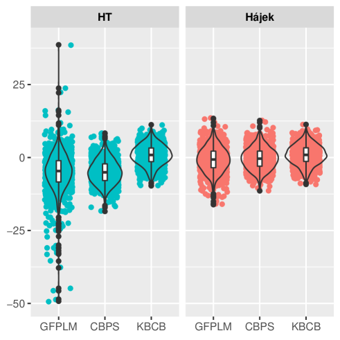
Figure 1: Violin plots for the 1,000 bootstrap HT and Hájek estimates for the average treatment effect of duloxitine on the VAS score.

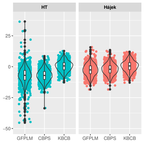
Figure 2: The same as Figure 1 except for the WOMAC score.

Tables 7 and 8 provide the HT and Hájek estimates, bootstrap standard errors and 95% bootstrap percentile confidence intervals for the average treatment effect of duloxitine on VAS and WOMAC scores respectively. They indicate no significant treatment effect of duloxitine over placebo pills on pain relief. This is consistent with Tétreault et al. (2016), although their conclusion was made from a double-blind clinical trial, i.e., the second trial, while we based our finding on an observational dataset. Explicitly, the 95% confidence intervals for the average treatment effect of duloxitine on VAS and WOMAC scores obtained from the double-blind trial are $[-8.402,6.760]$ and $[-9.717,8.832]$ respectively. Both confidence intervals are based on t statistics assuming normality of each treatment or control group and equal variances of the two groups, which are validated by the Shapiro-Wilk tests and F-tests respectively.

The $1,000$ bootstrap HT and Hájek average treatment effect estimates are illustrated in Figures 1 and 2 for VAS and WOMAC scores respectively. Both figures show that the HT estimates based on GFPLM for propensity score estimation have a much larger variation than the two covariate balancing methods, but inverse propensity score weighting can substantially reduce their differences as revealed by the Hájek estimates. The median of the Hájek estimates is shifted towards zero compared to that of the HT estimates when the propensity score is estimated by either GFPLM or CBPS. The two average treatment effect estimates essentially show no difference for KBCB.

6 Discussion

To the best of our knowledge, this paper has made the first attempt to study average treatment effect estimation via propensity score weighting for functional data in observational studies. The paper introduces both direct modeling and covariate balancing methods for propensity score estimation and systematically evaluates their performances via a simulation experiment and a real data application. The results confirm the benefits of both inverse propensity score weighting and covariate balancing methods as advocated for multivariate data.

The methods introduced in this paper for average treatment effect estimation only focus on the scenario where the outcome is a continuous scalar variable and there is only one functional covariate. However, with straightforward modifications, they may be generalized to handle multiple functional covariates and continuous functional outcomes.

The covariate balancing methods introduced above rely on a satisfactory multivariate substitute for the functional covariate, which requires the functional covariate to be either fully observed or densely measured (e.g., Dauxois et al., 1982; Hall and Hosseini-Nasab, 2006; Hall et al., 2006). A future research topic is to develop covariate balancing methods for sparsely measured functional covariates (e.g, James et al., 2000; Yao et al., 2005) or a unified approach for all types of functional covariates (e.g., Li and Hsing, 2010; Zhang and Wang, 2016; Liebl, 2019). Another interesting direction is to study non-truncation regularization methods, e.g., the roughness penalization, to solve covariate balancing equations with functional covariates.

References

- Abadie and Imbens (2006) Abadie, A. and G. W. Imbens (2006). Large sample properties of matching estimators for average treatment effects. Econometrica 74(1), 235–267.
- Belloni et al. (2017) Belloni, A., V. Chernozhukov, I. Fernández-Val, and C. Hansen (2017). Program evaluation and causal inference with high-dimensional data. Econometrica 85(1), 233–298.
- Belloni et al. (2014) Belloni, A., V. Chernozhukov, and C. Hansen (2014). Inference on treatment effects after selection among high-dimensional controls. The Review of Economic Studies 81(2), 608–650.
- Bosq (2000) Bosq, D. (2000). Linear processes in function spaces: theory and applications, Volume 149. Springer, New York.
- Cardot et al. (1999) Cardot, H., F. Ferraty, and P. Sarda (1999). Functional linear model. Statistics & Probability Letters 45(1), 11–22.
- Cardot et al. (2003) Cardot, H., F. Ferraty, and P. Sarda (2003). Spline estimators for the functional linear model. Statistica Sinica 13, 571–591.
- Chen et al. (2017) Chen, K., X. Zhang, A. Petersen, and H.-G. Müller (2017). Quantifying infinite-dimensional data: Functional data analysis in action. Statistics in Biosciences 9(2), 582–604.
- Chernozhukov et al. (2018) Chernozhukov, V., D. Chetverikov, M. Demirer, E. Duflo, C. Hansen, W. Newey, and J. Robins (2018). Double/debiased machine learning for treatment and structural parameters. The Econometrics Journal 21(1), C1–C68.
- Ciarleglio et al. (2015) Ciarleglio, A., E. Petkova, R. T. Ogden, and T. Tarpey (2015). Treatment decisions based on scalar and functional baseline covariates. Biometrics 71(4), 884–894.
- Ciarleglio et al. (2018) Ciarleglio, A., E. Petkova, T. Ogden, and T. Tarpey (2018). Constructing treatment decision rules based on scalar and functional predictors when moderators of treatment effect are unknown. Journal of the Royal Statistical Society: Series C (Applied Statistics) 67(5), 1331–1356.
- Cuevas (2014) Cuevas, A. (2014). A partial overview of the theory of statistics with functional data. Journal of Statistical Planning and Inference 147, 1–23.
- Cupidon et al. (2008) Cupidon, J., R. Eubank, D. Gilliam, and F. Ruymgaart (2008). Some properties of canonical correlations and variates in infinite dimensions. Journal of Multivariate Analysis 99(6), 1083–1104.
- Dauxois et al. (1982) Dauxois, J., A. Pousse, and Y. Romain (1982). Asymptotic theory for the principal component analysis of a vector random function: some applications to statistical inference. Journal of Multivariate Analysis 12(1), 136–154.
- Delicado et al. (2010) Delicado, P., R. Giraldo, C. Comas, and J. Mateu (2010). Statistics for spatial functional data: some recent contributions. Environmetrics 21(3-4), 224–239.
- Dubin and Müller (2005) Dubin, J. A. and H.-G. Müller (2005). Dynamical correlation for multivariate longitudinal data. Journal of the American Statistical Association 100(471), 872–881.
- Eubank and Hsing (2008) Eubank, R. L. and T. Hsing (2008). Canonical correlation for stochastic processes. Stochastic Processes and their Applications 118(9), 1634–1661.
- Farrell (2015) Farrell, M. H. (2015). Robust inference on average treatment effects with possibly more covariates than observations. Journal of Econometrics 189(1), 1–23.
- Ferraty and Vieu (2006) Ferraty, F. and P. Vieu (2006). Nonparametric functional data analysis: theory and practice. Springer, New York.
- Freedman and Berk (2008) Freedman, D. A. and R. A. Berk (2008). Weighting regressions by propensity scores. Evaluation Review 32(4), 392–409.
- Geenens (2011) Geenens, G. (2011). Curse of dimensionality and related issues in nonparametric functional regression. Statistics Surveys 5, 30–43.
- Greven and Scheipl (2017) Greven, S. and F. Scheipl (2017). A general framework for functional regression modelling. Statistical Modelling 17(1-2), 1–35.
- Guo (2004) Guo, W. (2004). Functional data analysis in longitudinal settings using smoothing splines. Statistical Methods in Medical Research 13(1), 49–62.
- Hainmueller (2012) Hainmueller, J. (2012). Entropy balancing for causal effects: A multivariate reweighting method to produce balanced samples in observational studies. Political Analysis 20(1), 25–46.
- Hall and Hosseini-Nasab (2006) Hall, P. and M. Hosseini-Nasab (2006). On properties of functional principal components analysis. Journal of the Royal Statistical Society: Series B (Statistical Methodology) 68(1), 109–126.
- Hall et al. (2006) Hall, P., H.-G. Müller, and J.-L. Wang (2006). Properties of principal component methods for functional and longitudinal data analysis. The Annals of Statistics 34(3), 1493–1517.
- Hansen (2004) Hansen, B. B. (2004). Full matching in an observational study of coaching for the sat. Journal of the American Statistical Association 99(467), 609–618.
- Hirano et al. (2003) Hirano, K., G. W. Imbens, and G. Ridder (2003). Efficient estimation of average treatment effects using the estimated propensity score. Econometrica 71(4), 1161–1189.
- Hörmann and Kokoszka (2012) Hörmann, S. and P. P. Kokoszka (2012). Functional time series. Handbook of Statistics: Time Series Analysis: Methods and Applications 30, 157–186.
- Horváth and Kokoszka (2012) Horváth, L. and P. Kokoszka (2012). Inference for functional data with applications, Volume 200. Springer, New York.
- Horvitz and Thompson (1952) Horvitz, D. G. and D. J. Thompson (1952). A generalization of sampling without replacement from a finite universe. Journal of the American Statistical Association 47(260), 663–685.
- Hsing and Eubank (2015) Hsing, T. and R. Eubank (2015). Theoretical foundations of functional data analysis, with an introduction to linear operators. John Wiley & Sons.
- Imai and Ratkovic (2014) Imai, K. and M. Ratkovic (2014). Covariate balancing propensity score. Journal of the Royal Statistical Society: Series B (Statistical Methodology) 76(1), 243–263.
- James et al. (2000) James, G., T. Hastie, and C. Sugar (2000). Principal component models for sparse functional data. Biometrika 87(3), 587–602.
- James (2002) James, G. M. (2002). Generalized linear models with functional predictors. Journal of the Royal Statistical Society: Series B (Statistical Methodology) 64(3), 411–432.
- Kang and Schafer (2007) Kang, J. D. Y. and J. L. Schafer (2007). Demystifying double robustness: A comparison of alternative strategies for estimating a population mean from incomplete data. Statistical Science 22(4), 523–539.
- Kokoszka and Reimherr (2017) Kokoszka, P. and M. Reimherr (2017). Introduction to functional data analysis. CRC Press.
- Kokoszka and Reimherr (2019) Kokoszka, P. and M. Reimherr (2019). Some recent developments in inference for geostatistical functional data. Revista Colombiana de Estadística 42(1), 101–122.
- Leurgans et al. (1993) Leurgans, S. E., R. A. Moyeed, and B. W. Silverman (1993). Canonical correlation analysis when the data are curves. Journal of the Royal Statistical Society. Series B (Methodological) 55(3), 725–740.
- Li et al. (2018) Li, F., K. L. Morgan, and A. M. Zaslavsky (2018). Balancing covariates via propensity score weighting. Journal of the American Statistical Association 113(521), 390–400.
- Li and Hsing (2010) Li, Y. and T. Hsing (2010). Uniform convergence rates for nonparametric regression and principal component analysis in functional/longitudinal data. The Annals of Statistics 38(6), 3321–3351.
- Lian (2014) Lian, H. (2014). Some asymptotic properties for functional canonical correlation analysis. Journal of Statistical Planning and Inference 153, 1–10.
- Liebl (2019) Liebl, D. (2019). Inference for sparse and dense functional data with covariate adjustments. Journal of Multivariate Analysis 170, 315–335.
- Lindquist (2012) Lindquist, M. A. (2012). Functional causal mediation analysis with an application to brain connectivity. Journal of the American Statistical Association 107(500), 1297–1309.
- Marron and Alonso (2014) Marron, J. S. and A. M. Alonso (2014). Overview of object oriented data analysis. Biometrical Journal 56(5), 732–753.
- McKeague and Qian (2014) McKeague, I. W. and M. Qian (2014). Estimation of treatment policies based on functional predictors. Statistica Sinica 24(3), 1461–1485.
- McLean et al. (2014) McLean, M. W., G. Hooker, A.-M. Staicu, F. Scheipl, and D. Ruppert (2014). Functional generalized additive models. Journal of Computational and Graphical Statistics 23(1), 249–269.
- Morris (2015) Morris, J. S. (2015). Functional regression. Annual Review of Statistics and Its Application 2(1), 321–359.
- Müller (2008) Müller, H.-G. (2008). Functional modeling of longitudinal data. In Longitudinal Data Analysis, pp. 237–266. Chapman and Hall/CRC.
- Müller and Stadtmüller (2005) Müller, H.-G. and U. Stadtmüller (2005). Generalized functional linear models. the Annals of Statistics 33(2), 774–805.
- Müller et al. (2013) Müller, H.-G., Y. Wu, and F. Yao (2013). Continuously additive models for nonlinear functional regression. Biometrika 100(3), 607–622.
- Nagy (2017) Nagy, S. (2017). An overview of consistency results for depth functionals. In Functional Statistics and Related Fields, pp. 189–196. Springer.
- Ning et al. (2018) Ning, Y., S. Peng, and K. Imai (2018). Robust estimation of causal effects via high-dimensional covariate balancing propensity score. arXiv preprint arXiv:1812.08683.
- Paganoni and Sangalli (2017) Paganoni, A. M. and L. M. Sangalli (2017). Functional regression models: Some directions of future research. Statistical Modelling 17(1-2), 94–99.
- Qin and Zhang (2007) Qin, J. and B. Zhang (2007). Empirical-likelihood-based inference in missing response problems and its application in observational studies. Journal of the Royal Statistical Society: Series B (Statistical Methodology) 69(1), 101–122.
- Ramsay and Silverman (2005) Ramsay, J. O. and B. W. Silverman (2005). Functional data analysis (2nd ed.). New York: Springer.
- Reiss et al. (2017) Reiss, P. T., J. Goldsmith, H. L. Shang, and R. T. Ogden (2017). Methods for scalar-on-function regression. International Statistical Review 85(2), 228–249.
- Robins et al. (2000) Robins, J. M., M. Á. Hernán, and B. Brumback (2000). Marginal structural models and causal inference in epidemiology. Epidemiology 11(5), 550–560.
- Robins et al. (1994) Robins, J. M., A. Rotnitzky, and L. P. Zhao (1994). Estimation of regression coefficients when some regressors are not always observed. Journal of the American Statistical Association 89(427), 846–866.
- Rosenbaum (1987) Rosenbaum, P. R. (1987). Model-based direct adjustment. Journal of the American Statistical Association 82(398), 387–394.
- Rosenbaum (1989) Rosenbaum, P. R. (1989). Optimal matching for observational studies. Journal of the American Statistical Association 84(408), 1024–1032.
- Rosenbaum (1991) Rosenbaum, P. R. (1991). A characterization of optimal designs for observational studies. Journal of the Royal Statistical Society: Series B (Methodological) 53(3), 597–610.
- Rosenbaum and Rubin (1983) Rosenbaum, P. R. and D. B. Rubin (1983). The central role of the propensity score in observational studies for causal effects. Biometrika 70(1), 41–55.
- Rosenbaum and Rubin (1984) Rosenbaum, P. R. and D. B. Rubin (1984). Reducing bias in observational studies using subclassification on the propensity score. Journal of the American Statistical Association 79(387), 516–524.
- Rosenbaum and Rubin (1985) Rosenbaum, P. R. and D. B. Rubin (1985). Constructing a control group using multivariate matched sampling methods that incorporate the propensity score. The American Statistician 39(1), 33–38.
- Rubin (2007) Rubin, D. B. (2007). The design versus the analysis of observational studies for causal effects: parallels with the design of randomized trials. Statistics in Medicine 26(1), 20–36.
- Shang (2014) Shang, H. L. (2014). A survey of functional principal component analysis. AStA Advances in Statistical Analysis 98(2), 121–142.
- Shin (2009) Shin, H. (2009). Partial functional linear regression. Journal of Statistical Planning and Inference 139(10), 3405–3418.
- Shin and Lee (2015) Shin, H. and S. Lee (2015). Canonical correlation analysis for irregularly and sparsely observed functional data. Journal of Multivariate Analysis 134, 1–18.
- Smith and Todd (2005) Smith, J. A. and P. E. Todd (2005). Does matching overcome lalonde’s critique of nonexperimental estimators? Journal of Econometrics 125(1-2), 305–353.
- Tétreault et al. (2016) Tétreault, P., A. Mansour, E. Vachon-Presseau, T. J. Schnitzer, A. V. Apkarian, and M. N. Baliki (2016). Brain connectivity predicts placebo response across chronic pain clinical trials. PLoS Biology 14(10), e1002570.
- Vieu (2018) Vieu, P. (2018). On dimension reduction models for functional data. Statistics & Probability Letters 136, 134–138.
- Wang et al. (2016) Wang, J.-L., J.-M. Chiou, and H.-G. Müller (2016). Functional data analysis. Annual Review of Statistics and Its Application 3, 257–295.
- Wong and Chan (2018) Wong, R. K. and K. C. G. Chan (2018). Kernel-based covariate functional balancing for observational studies. Biometrika 105(1), 199–213.
- Yao et al. (2005) Yao, F., H.-G. Müller, and J.-L. Wang (2005). Functional data analysis for sparse longitudinal data. Journal of the American Statistical Association 100(470), 577–590.
- Yuan and Cai (2010) Yuan, M. and T. T. Cai (2010). A reproducing kernel hilbert space approach to functional linear regression. The Annals of Statistics 38(6), 3412–3444.
- Zhang and Chen (2007) Zhang, J.-T. and J. Chen (2007). Statistical inferences for functional data. The Annals of Statistics 35(3), 1052–1079.
- Zhang and Wang (2016) Zhang, X. and J.-L. Wang (2016). From sparse to dense functional data and beyond. The Annals of Statistics 44(5), 2281–2321.
- Zhao (2019) Zhao, Q. (2019). Covariate balancing propensity score by tailored loss functions. The Annals of Statistics 47(2), 965–993.
- Zhao and Luo (2019) Zhao, Y. and X. Luo (2019). Granger mediation analysis of multiple time series with an application to functional magnetic resonance imaging. Biometrics 75(3), 788–798.
- Zhao et al. (2018) Zhao, Y., X. Luo, M. Lindquist, and B. Caffo (2018). Functional mediation analysis with an application to functional magnetic resonance imaging data. arXiv preprint arXiv:1805.06923.
- Zhou et al. (2018) Zhou, Y., S.-C. Lin, and J.-L. Wang (2018). Local and global temporal correlations for longitudinal data. Journal of Multivariate Analysis 167, 1–14.
- Zubizarreta (2015) Zubizarreta, J. R. (2015). Stable weights that balance covariates for estimation with incomplete outcome data. Journal of the American Statistical Association 110(511), 910–922.