Digging for relics of the past: the ancient and obscured bulge globular cluster NGC 6256

Abstract

We used a set of moderately-deep and high-resolution optical observations obtained with the Hubble Space Telescope to investigate the properties of the stellar population in the heavily obscured bulge globular cluster NGC 6256. The analysis of the color-magnitude diagram revealed a stellar population with an extended blue horizontal branch and severely affected by differential reddening, which was corrected taking into account color excess variations up to $\delta E(B-V)\sim 0.51$. We implemented a Monte Carlo Markov Chain technique to perform the isochrone fitting of the observed color-magnitude diagram in order to derive the stellar age, the cluster distance and the average color excess in the cluster direction. Using different set of isochrones we found that NGC 6256 is characterised by a very old stellar age around $13.0$ Gyr, with a typical uncertainty of $\sim 0.5$ Gyr. We also found an average color excess $E(B-V)=1.19$ and a distance from the Sun of 6.8 kpc. We then derived the cluster gravitational center and measured its absolute proper motion using the Gaia-DR2 catalog. All this was used to back-integrate the cluster orbit in a Galaxy-like potential and measure its integrals of motion. It turned out that NGC 6256 is currently in a low-eccentricity orbit entirely confined within the bulge and its integrals of motion are fully compatible with a cluster purely belonging to the Galaxy native globular cluster population. All these pieces of evidence suggest that NGC 6256 is an extremely old relic of the past history of the Galaxy, formed during the very first stages of its assembly.

1 Introduction

Bulge globular clusters (GCs) are ideal tools to trace the properties (kinematics, chemistry and age) of the stellar populations located in the inner regions of the Galaxy. However, their observation is highly challenging, not only because they are situated in a distant and very crowded region of the Milky Way, but also because they are usually affected by severe and differential extinction, due to the large and patchy amount of interposed interstellar dust. This is the reason why most of the bulge GCs are still poorly studied. The current picture is that a handful of bulge GCs is characterized by a relatively low metal content ([Fe/H]$<-1.0$) with respect to the metallicities typically observed for the majority of both GCs and field stars residing in the bulge (e.g., Bica et al., 2016). This value of [Fe/H], together with the significant $\alpha$ enhancement ([$\alpha/$Fe]$\geq 0.3$) measured in these systems, suggests that they have been generated through an early and fast star formation burst during the initial stages of the Galaxy assembly (see, e.g., Cescutti et al., 2008). Interestingly, the first age measurements of some of these relatively metal-poor systems suggested that they are indeed very old, with ages around 13 Gyr (see, e.g., the cases of NGC 6522, HP1 and Djorgovski 2; Kerber et al., 2018, 2019; Ortolani et al., 2019b). More in general, improved age estimates of bulge GCs are tentatively suggesting the presence of a correlation between the age and the metallicity of these systems, with the more metal-poor clusters being older than the more metal-rich ones (see Figure 16 in Saracino et al., 2019). A deep investigation of these systems is thus crucial to constrain the slope of the presumed age-[Fe/H] relation, which is still completely unknown, but could bring precious information on the bulge formation processes.

This work is part of an ongoing large program aimed at characterizing the stellar populations of highly extincted stellar systems orbiting within the Galactic bulge, which led us to the discovery of the surprising properties of the stellar system Terzan 5 (see Ferraro et al., 2009, 2015, 2016; Lanzoni et al., 2010; Origlia et al., 2011, 2013, 2019; Massari et al., 2012, 2014a, 2014b; Cadelano et al., 2018) and other intriguing clusters (Saracino et al., 2015, 2016, 2019; Pallanca et al., 2019). This paper focused on NGC 6256. So far, only a handful of photometric and spectroscopic works have attempted to constrain its properties, and a reliable and comprehensive characterization of this system is thus still lacking. One of the first photometric studies showing the optical color-magnitude diagram (CMD) of the cluster was presented by Alcaino (1983), who suggested that NGC 6256 is a metal-rich cluster similar to 47 Tucanae, located at 11 kpc from the Sun and with a large color excess of $E(B-V)=0.8$. Different results were then found by Webbink (1985), who estimated a much lower metallicity for this system ([Fe/H]$\approx-1.56$), a slightly smaller distance ($d=9.1$ kpc), and a color-excess $E(B-V)=0.88$. Deeper optical studies (Ortolani et al., 1999) revised again the situation, suggesting that NGC 6256 presents a blue horizontal branch, an intermediate metallicity ([Fe/H]$\approx-1.3$), a distance of just 6.4 kpc, and an even larger color excess, $E(B-V)=1.1$. The first high resolution study of the system, performed through Hubble Space Telescope (HST) observations by Piotto et al. (2002), revealed very scattered red giant branch and horizontal branch stars, hinting to the presence of significant variations of the color excess even within the small field of view covered by the observations. Finally, the ground-based near-IR photometric investigation performed by Valenti et al. (2007) with the ESO-NTT found [Fe/H]$=-1.63$, a distance modulus $(m-M)_{0}=14.79$ (corresponding to 9.1 kpc) and $E(B-V)=1.2$, while the compilation by Harris (2010) quotes [Fe/H]$=-1.02$, $d=10.3$ kpc, and $E(B-V)=1.09$. A recent spectroscopic analysis of ten giant stars (Vásquez et al., 2018, but see also Stephens & Frogel 2004) revealed that the stellar population of NGC 6256 is characterized by [Fe/H]$\approx-1.61$, with a possible intrinsic dispersion of 0.2 dex, implying that NGC 6256 is one of the metal-poorest GC currently located within the Galactic bulge.

These results clearly demonstrate that a detailed and reliable physical characterization of this cluster is still lacking. Indeed, even the most recent Gaia DR2 data (Gaia Collaboration et al., 2016) are useless to this aim, because of the large reddening and crowding conditions in the direction of the system, and they can just provide the proper motion of the brightest stars (Baumgardt et al., 2019). The goal of this study is thus to obtain a coherent view of the properties of the stellar population in the inner regions of NGC 6256. To this end, we make use of a set of moderately-deep and high-resolution images acquired with the HST. In Section 2, the data-set and the data reduction procedure are described; in Section 3 we discuss the differential reddening correction; in Section 4 and 5 we present the determination of the cluster stellar population properties and of its orbit within the Galaxy. Finally, in Section 6, we summarize the results and draw our conclusions.

2 Observations and Data analysis

This work is based on a set of high-resolution optical observations obtained with the Wide Field Camera 3 (WFC3) on board the HST, under GO 11628 (PI: Noyola). It consists of 3 images acquired with the F555W filter and exposure time of 360 s, and 3 images in the F814W filter with exposure time of 100 s. The photometric analysis was performed with DAOPHOT IV (Stetson, 1987) on the dark, bias, flat and charge transfer efficiency corrected “flc” images (see e.g. Cadelano et al., 2017b, 2019). As a first step, about 200 stars were selected in each image in order to model the point spread function (PSF), whose full width at half maximum was set to 1.5 pixels ($\sim 0.06\arcsec$) and sampled within a radius of 10 pixels ($\sim 0.4\arcsec$). The PSF models were chosen on the basis of a $\chi^{2}$ statistic and, in every image, the best-fit was provided by a Moffat function (Moffat, 1969). These models were finally applied to all the sources detected at more than $5\sigma$ from the background level in each image. Then, we built a master catalog with stars detected in at least 2 of the available images per filter. At the corresponding positions of these stars, the photometric fit was forced in all the other frames by using DAOPHOT/ALLFRAME (Stetson, 1994). Finally, for each star we homogenized the magnitudes estimated in different images, and their weighted mean and standard deviation were adopted as the star magnitudes and their related photometric errors. Instrumental magnitudes have been reported to the VEGAMAG system by using the zero-points values for an aperture of 10 pixels, as quoted in the WFC3 website’: $ZP_{\rm F555W1}=25.735$, $ZP_{\rm F555W2}=25.720$ for the F555W magnitudes of stars observed in chip 1 and in chip 2 of the camera, respectively, and $ZP_{\rm F814W1}=24.598$ and $ZP_{\rm F814W2}=24.574$ for the corresponding F814W magnitudes. Finally, we applied appropriate aperture corrections, evaluated independently for each chip and filter at a radius of 10 pixels from the stellar centers. The aperture corrections are of the order of $-0.03$ mags for both the chips in the F555W observations, and around $-0.01$ mags for both the chips of the F814W images.

The instrumental positions have been corrected for geometric distortions following the procedure described by Bellini et al. (2011). They have been then reported to the absolute coordinate system by cross-correlation with the Gaia DR2 publicly available catalog (Gaia Collaboration et al., 2018).

The resulting CMD of the cluster is reported in the left panel of Figure 1, where it can be appreciated an important broadening of all the evolutionary sequences due to severe differential reddening affecting the whole field of view ($\sim 160\arcsec\times 160\arcsec$).

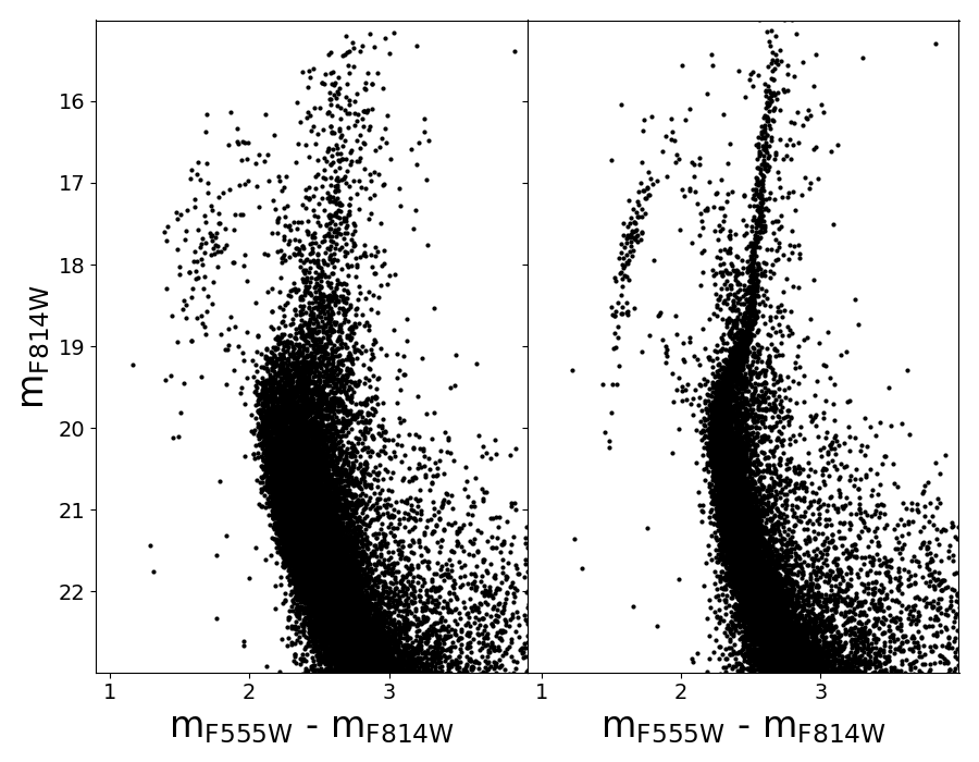
Figure 1: Left panel: Optical CMD of NGC 6256 obtained from the HST data-set used in this work. Right panel: same as in the left panel, but after the correction for differential reddening (see Section 3).

3 Differential reddening correction

For a proper derivation of the cluster population properties, it is first necessary to correct the stellar magnitudes for the effects of the strong differential reddening affecting the field of view. To do this, we used an approach similar to that described in Dalessandro et al. (2018) and Saracino et al. (2019, see also , ). First of all, we created the cluster mean ridge line (MRL). We roughly selected a sample of likely cluster member stars along the main-sequence, sub-giant and red giant branches based on their observed position in the CMD. The resulting sample is plotted with black points in the left panel of Figure 2. To minimize the contamination from field stars, we further selected only the stars located within the cluster half-light radius ($\sim 50\arcsec$) quoted in Harris (2010). We then iteratively divided the CMD in magnitude bins of different widths, ranging from 0.15 to 0.5 mags in steps of 0.01 mags. During each iteration, at a fixed bin width, we evaluated the sigma-clipped mean color of the selected sample within each bin and determined a MRL by connecting all these values together. Finally, at the end of the iterations, we averaged all these MRLs to obtain the final MRL shown in the left panel of Figure 2.

For the stars belonging to the sample of likely cluster members in the magnitude range $16<m_{\rm F814W}<21$, and independently of their distance from the center, we computed their distance ($\Delta X$) from the MRL along the reddening vector, defined using the extinction coefficients $R_{\rm F555W}=3.207$ and $R_{\rm F814W}=1.842$, appropriate for turn-off stars ($T_{\rm eff}\sim 6000$ K) and obtained from Cardelli et al. (1989) and Girardi et al. (2002).

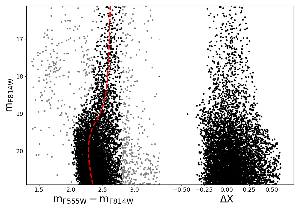
Figure 2: Left panel: Zoomed view of the cluster CMD (the same as the one plotted in the left panel of Figure 1). Black points are the stars roughly selected as cluster members and used to determine the cluster MRL, which is shown as a dashed red curve. Right panel: stellar magnitudes as a function of their distance from the MRL ($\Delta X$) for the reference sample used for the differential reddening determination (black points on the left panel).

The resulting distribution of $\Delta X$ as a function of the stellar magnitude is shown in the right panel of Figure 2. This reference sample was used to assign a value of $\Delta X$ to all the sources in our photometric catalog, as follows. For each source, $\Delta X$ and its uncertainty were determined as the $\sigma$-clipped median and standard deviation of the $\Delta X$ values measured for the $n$ closest reference stars. The resulting values of $\Delta X$ (and related uncertainties) can be transformed into the local differential reddening $\delta E(B-V)$ and used to correct the observed stellar magnitudes by using the following equation:

$$\delta E(B-V)=\frac{\Delta X}{\sqrt{R_{\rm F555W}^{2}-2R_{\rm F555W}R_{\rm F814W}+2R_{\rm F814W}^{2}}},$$ (1)

This procedure was iterated three times. Initially, $\Delta X$ was measured for each star using the 30 closest reference stars, then using the 25 and finally the 20 closest stars. These numbers have been chosen as a compromise between having enough statistic and achieving good enough spatial resolution in the final reddening map. The procedure was stopped at the third iteration, as a fourth one would introduce magnitude corrections negligible with respect to the photometric errors.

At the end of the procedure, we found reddening variations within the surveyed field as large as $\delta E(B-V)=0.51$. The detailed spatial distribution of the reddening variations is shown in the map plotted in Figure 3. This reddening correction, applied to all the stars in the catalog, resulted in the CMD shown in right panel of Figure 1. As can be seen, the evolutionary sequences are now significantly better outlined: indeed, the sub-giant branch, the red giant branch and an extended blue horizontal branch can now be clearly appreciated, and the main sequence is also much thinner. The CMD also reveals that NGC 6256 suffers from a large contamination from field interlopers, that cannot be removed with the available data-sets because of their limited time baseline, which make them not suitable to perform proper motion analysis.

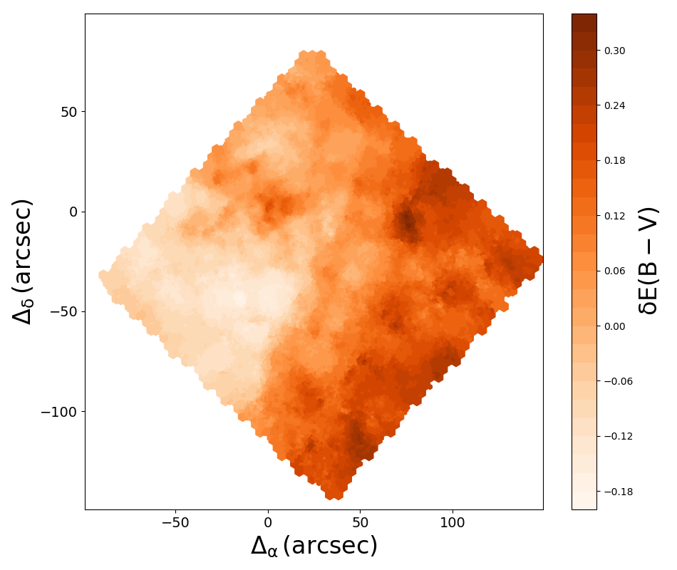
Figure 3: Differential reddening map within the observed field of view in the direction of NGC 6256. Positions are reported with respect to the cluster center. Different colors correspond to different values of $\delta E(B-V)$, as reported in the color-bar on the right.

4 Age, distance and color excess determination

4.1 First-guess estimates of distance and color excess

The differential reddening-corrected CMD discussed above has been used to determine the cluster properties (distance, absolute color excess, and stellar population age) via isochrone fitting. To this aim, it is helpful to obtain an independent estimates of both the cluster distance modulus and color excess, to be used as starting point in the isochrone fitting procedure. As discussed in Section 1, the values for these parameters available in the literature are still extremely uncertain.

Unfortunately, no RRLyrae stars (that would be suitable to determine the distance modulus) are known in this cluster. Moreover, the publicly available parallaxes in the Gaia Data Release 2 (DR2) catalog (Gaia Collaboration et al., 2018) are extremely uncertain for the stars in the direction of this cluster and they cannot be used to constrain the cluster distance. The same holds for the absolute color excess: the spatial resolution of the publicly available all-sky maps of interstellar extinction (e.g. Schlafly, & Finkbeiner, 2011) are too poor to get a reliable average value of this parameter, given the extreme variations on very small scales shown in Figure 3.

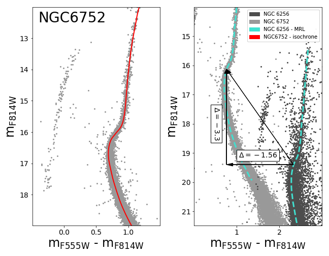
Figure 4: Left panel: $m_{\rm F814W},(m_{\rm F555W}-m_{\rm F814W})$ CMD of NGC 6752. The red line is a DSED isochrone with an age of 13 Gyr, reported into the observational plane by assuming $E(B-V)=0.04$ and $(m-M)_{0}=13.14$. Right panel: The dark gray dots show the same CMD of NGC 6256 as in Figure 1, while the light gray dots show the same NGC 6752 CMD as in the left panel. The cyan dashed curve is the MRL derived in Section 3. The adopted shifts in color and magnitude are marked with the two black arrows.

We thus estimated the cluster distance modulus and average color excess by comparing the observed CMD with a catalog of stars of the GC NGC 6752, obtained from images acquired under GO 11904 (PI: Kalirai) with the same instrument and combination of filters as for NGC 6256. The data reduction and calibration of these images is exactly the same as the one described in Section 2.

NGC 6752 is a $\sim 13$ Gyr old system (Gratton et al., 2003; Dotter et al., 2010), with a metallicity [Fe/H]$=-1.56\pm 0.04$ (Carretta et al., 2009) comparable to that of NGC 6256, and very well constrained distance modulus and color excess: $(m-M)_{0}=13.14\pm 0.06$ and $E(B-V)=0.04\pm 0.01$ (Baumgardt et al., 2019; Ferraro et al., 1999). For two systems with approximately the same metallicity and age, it is expected that any magnitude difference between their MRLs is mainly due to the relative difference in distance and color excess. The left panel of Figure 4 shows that, assuming the metallicity, distance modulus, and color excess quoted above for NGC 6752, a 13 Gyr isochrone extracted from the Dartmouth Stellar Evolutionary Database (DSED; Dotter et al., 2008) provides a good match of the cluster CMD. We then applied color and magnitude shifts to the MRL of NGC 6256 obtained in Section 3 (cyan dashed line in the right panel of Figure4) to superimpose it onto the MRL of NGC 6752 (created using the same procedure described in Section 3). To do this, we performed a fit of the two curves in the magnitude range $15<m_{\rm F814W}<18$ and chose the best-fit shifts on the basis of the $\chi^{2}$ statistics, finding $\Delta(m_{\rm F555W}-m_{\rm F814W})=-1.56$ and $\Delta m_{\rm F814W}=-3.3$. Adopting the same extinction coefficients used in Section 3, these shifts corresponds to a color excess $E(B-V)=1.18\pm 0.05$ and a distance modulus $(m-M)_{0}=14.25\pm 0.1$ for NGC 6256. We stress that these are only first-guess estimates, just used as starting points for the accurate isochrone fitting of the cluster CMD discussed in the next Section. In fact, these relative measurements could be biased by the possible differences in the cluster’s relative age and in the light-element abundances of the cluster’s sub-populations. Moreover, these results could also be biased by the effects of a very different $E(B-V)$ on the observed sequences (see Section 4.2 and Figure 5).

4.2 Isochrone fitting

To derive the absolute age of the cluster via isochrone fitting, we followed a Bayesian procedure similar to that used by Saracino et al. (2019, see also , ). This approach allows to estimate the stellar system age through a one-to-one comparison between the observed CMD and a set of theoretical models, simultaneously exploring reasonable grids of values for the relevant cluster parameters (not only the age, but also the distance modulus and color excess).

The observed CMD was compared to three different sets of $\alpha$-enhanced isochrones: the DSED models (Dotter et al., 2008), the Victoria-Regina Isochrone Database (VR, VandenBerg et al., 2014) and the BaSTI stellar evolution models (Pietrinferni et al., 2004, 2006). For each family of models we assumed [$\alpha/$Fe]$=+0.4$, which is the typical value for bulge GCs, and a standard He abundance $Y=0.25$. In the case of the DSED and VR databases, isochrones can be generated at different metallicities, while for the BaSTI database only a selection of [Fe/H] values is available. Therefore, in order to perform a proper comparison between the results obtained from these different models, we assumed in all cases [Fe/H]$=-1.62$, a value which is extremely close to that derived through spectroscopy (Vásquez et al., 2018) and that is available for all the three sets of models. The adopted extinction coefficients in the F555W and F814W bands take into account the dependence of the reddening on the effective temperature of the stars, following the extinction laws of Cardelli et al. (1989), the equations in Girardi et al. (2002) and assuming the alpha-enhanced spectral library used in Pietrinferni et al. (2006). This is indeed necessary for performing reliable isochrone fitting in the case of highly reddened systems, because neglecting such a temperature dependence makes the red giant branch and the main sequence shallower, thus increasing the overall color range spanned by the isochrone in the CMD. This is shown in Figure 5, where we plot, as an example, the same DSED isochrone (with an age of 12.5 Gyr, [Fe/H]$=-1.62$ and the first-guess values of distance modulus and $E(B-V)$ estimated for NGC 6256 in the previous Section) before and after such a correction: the black line corresponds to the isochrone obtained by using constant extinction coefficients ($R_{\rm F555W}=3.207$ and $R_{\rm F814W}=1.842$), while the red line is derived by correcting the extinction coefficients for the dependence on the surface temperature of the stars. As can be seen, the significant color difference between the two curves demonstrates that reliable age estimates for heavily reddened systems, such as NGC 6256, cannot be performed by assuming constant extinction coefficients, especially when dealing with optical filters (in fact, this effect is larger for decreasing wavelengths).

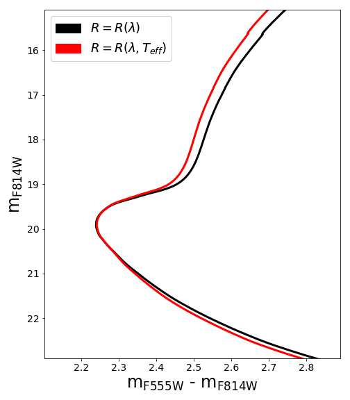
Figure 5: The black curve is a DSED isochrone computed for a stellar population of 12.5 Gyr and [Fe/H]$=-1.62$, in the same filter combination used in this work. It has been put into the observational plane by using a distance modulus of 14.25, a color excess $E(B-V)=1.18$, and constant extinction coefficients: $R_{\rm F555W}=3.207$ and $R_{\rm F814W}=1.842$. The red curve is the same isochrone, but with temperature-dependent extinction coefficients.

To compare the observed CMD of NGC 6256 with the three families of stellar models we applied a Markov Chain Monte Carlo (MCMC) sampling technique. We assumed that the probability of a $n^{th}$ star to belong to an isochrone (corrected for a given reddening and distance) can be expressed in terms of a Gaussian distribution:

$$p_{n}=\frac{1}{\sqrt{2\pi}\sigma_{n}}\exp{\left[-\frac{1}{2}\frac{d_{n}^{2}}{\sigma_{n}^{2}}\right]}\propto\frac{\exp{\left(-\frac{d_{n}^{2}}{2\sigma_{n}^{2}}\right)}}{\sigma_{n}}$$ (2)

where $d_{n}$ is the minimum distance of the star from the isochrone and $\sigma_{n}$ the uncertainty of such a distance expressed as $\sigma=\sqrt{\sigma_{col}^{2}+\sigma_{mag}^{2}+\sigma_{DR}^{2}}$, where $\sigma_{col}$, $\sigma_{mag}$ are the photometric uncertainties on the color and F814W magnitude, respectively, while $\sigma_{DR}$ are the uncertainties on the differential correction derived as discussed in Section 3. Therefore, the logarithmic likelihood function of a given isochrone can be expressed as the logarithm of the sum of $p_{n}$ over all the $n^{th}$ stars:

$$\ln\mathscr{L}=\ln\sum_{n=1}^{N_{stars}}p_{n}\propto-\frac{1}{2}\sum_{n=1}^{N_{stars}}\left[\frac{d_{n}^{2}}{\sigma_{n}^{2}}+\ln(\sigma_{n}^{2})\right]$$ (3)

To sample the posterior probability distribution in the n-dimensional parameter space, we used the emcee code (Foreman-Mackey et al., 2019). Since no age estimates are available in the literature for NGC 6256, we explored a wide range of old ages, uniformly distributed from 10 to 15 Gyr, in steps of 0.25 Gyr. To put the isochrones into the observational plane, we used values of the color excess and distance modulus following Gaussian prior distributions peaked at $E(B-V)=1.2\pm 0.1$ and $(m-M)_{0}=14.25\pm 0.1$, respectively. In order to minimize the contamination by field interlopers, we extended these calculations only to stars within the cluster half-light radius ($\sim 50\arcsec$; Harris, 2010). Moreover, we restricted the analysis only to stars in the magnitude range $18.5<m_{F814W}<20.5$, a CMD region surrounding the turn-off and therefore sensitive to stellar age variations.

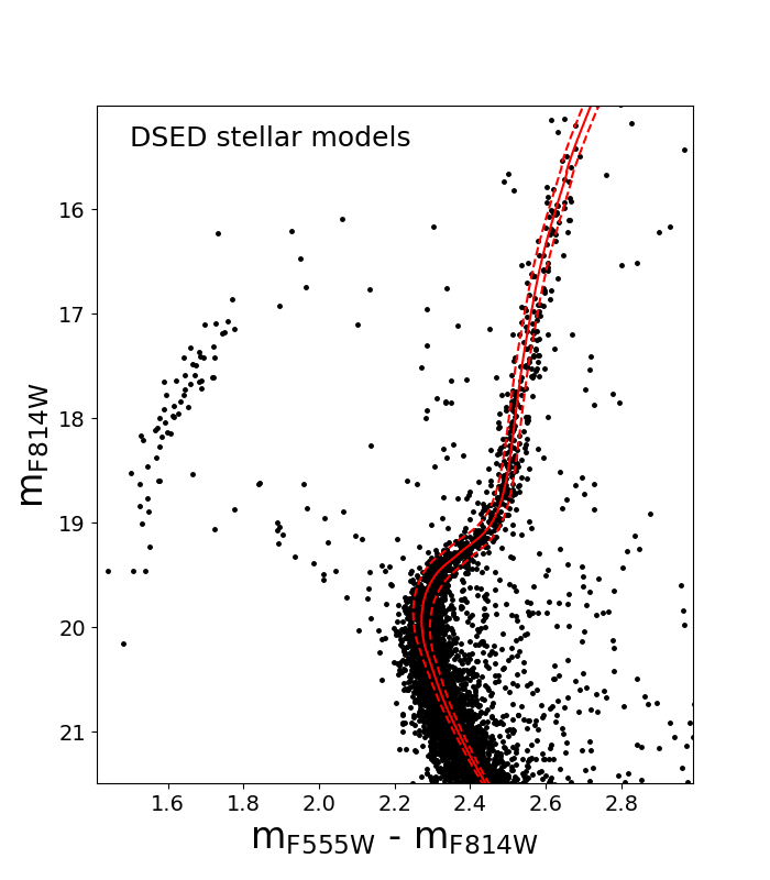
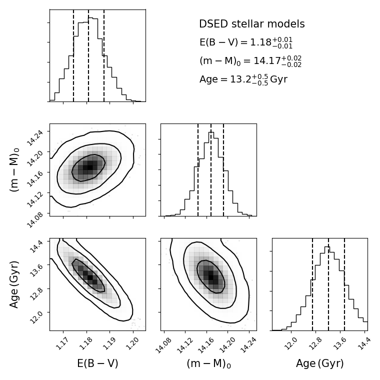
Figure 6: Left panel: CMD of NGC 6256 with the best-fit DSED isochrone plotted as a red solid line. All the solutions within the $1\sigma$ uncertainties are confined in the region between the two dashed red isochrones. Right panel: Corner plots showing the one- and two-dimensional projections of the posterior probability distributions for all the parameters derived from the MCMC method applied to the DSED model family. The contours correspond to the 1$\sigma$, 2$\sigma$ and 3$\sigma$ levels. The best-fit parameter values are presented in Table 1.

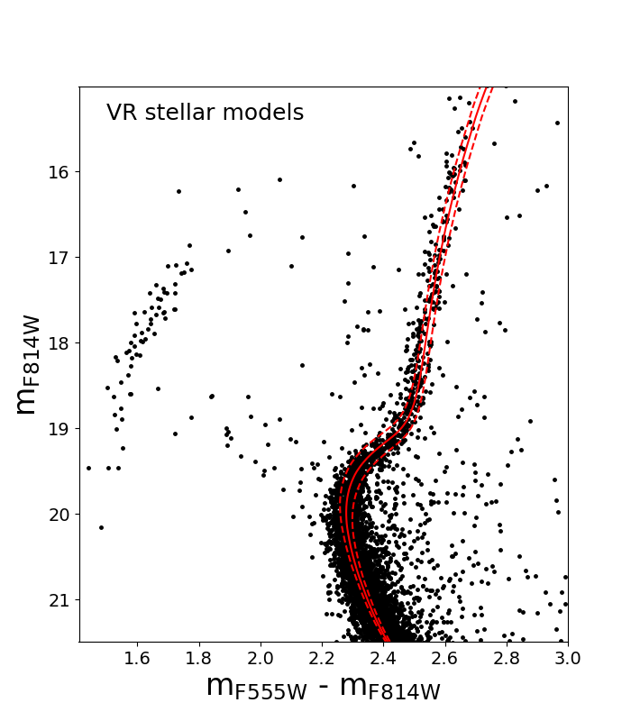
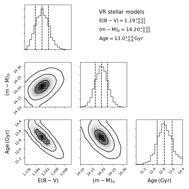
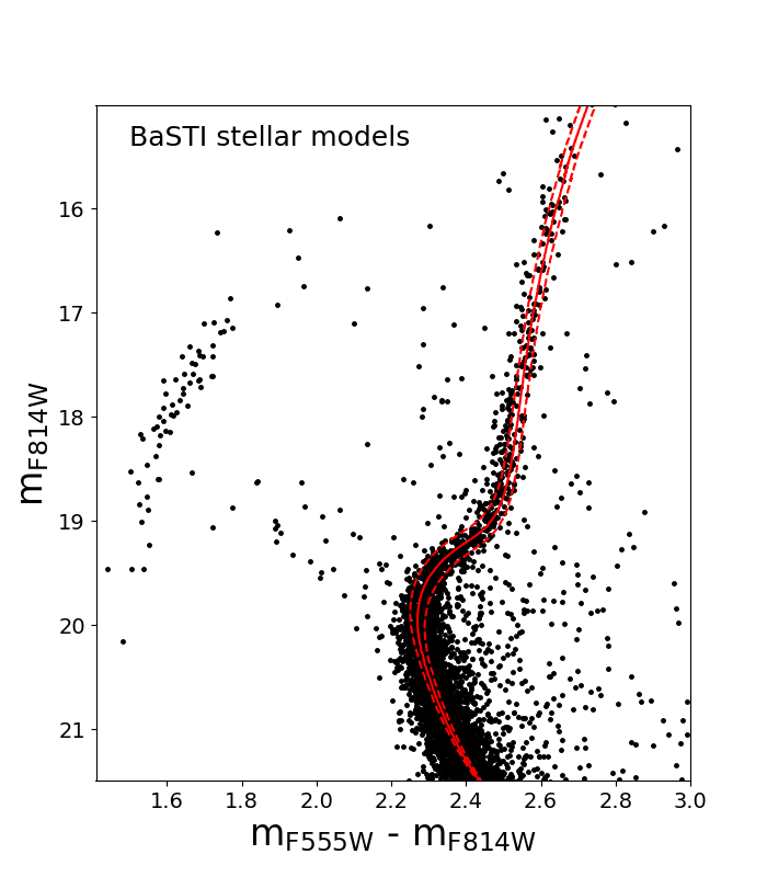
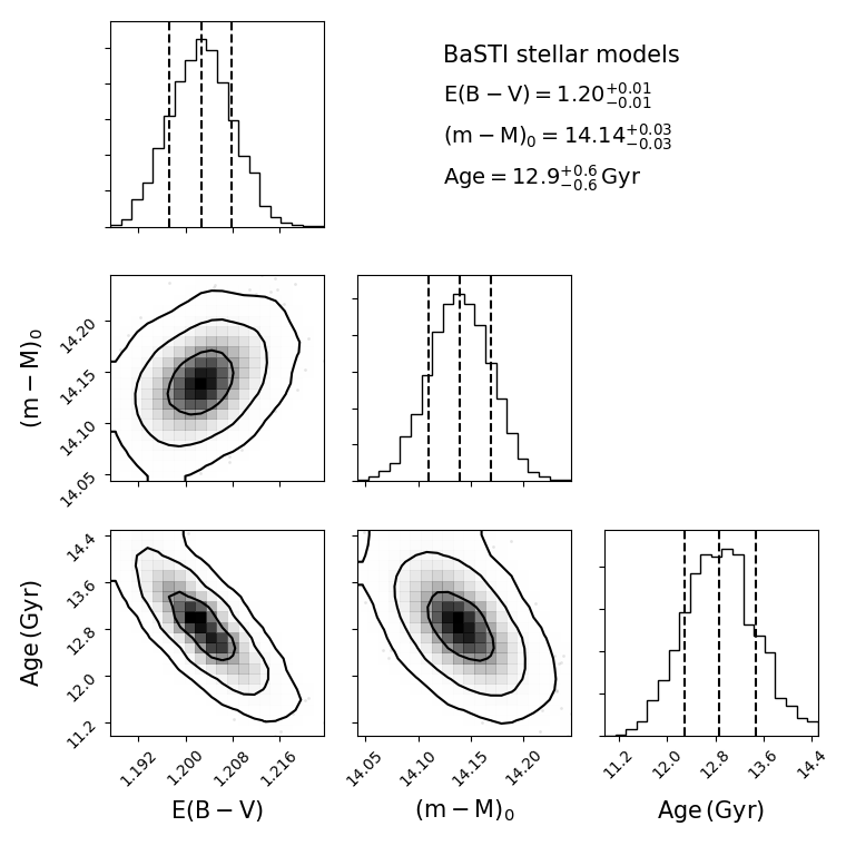
Figure 7: As in Figure 6, but for the VR models (top panels) and the BaSTI models (bottom panels). The best-fit parameter values are presented in Table 1.

The results obtained in terms of age, distance modulus and color excess are shown in Figures 6 and 7 for the three adopted sets of theoretical models. In each figure, the left-hand panel shows the $(m_{\rm F814W},m_{\rm F555W}-m_{\rm F814W})$ CMD and the best-fit isochrones. In all the cases, the best-fit model very well reproduces the cluster evolutionary sequences. The one- and two-dimensional posterior probabilities for all of the parameter combinations are presented in the right-hand panels as corner plots. The best-fit values and their uncertainties (based on the $16^{th}$, $50^{th}$, $84^{th}$ percentiles) obtained for the age, $E(B-V)$ and $(m-M)_{0}$ from the three sets of models are also listed in Table 1. Since we are using different models (adopting slightly different solar abundances, opacities, reaction rates, efficiency of atomic diffusion etc.), the resulting best-fit values are somewhat expected to be not exactly the same. However, they are all mutually consistent within the errors. NGC 6256 turns out to be a very old cluster, with an age of 13.0 Gyr (obtained as the average of the three derived values). The average color excess, $E(B-V)=1.19$, is in good agreement with that quoted by Valenti et al., 2007, and it implies that, within the field of view covered by our observations, this parameter varies from a minimum of $\sim 1.0$ up to $\sim 1.5$. The obtained distance modulus corresponds to a distance of $6.8\pm 0.1$ kpc from the Sun and turns out to be significantly different from some of the values quoted in literature. Indeed, the cluster results 3.5 kpc closer than reported in Harris (2010) and 2.3 kpc closer than the value quoted in Valenti et al. (2007).

Table 1: Best-fit parameter values for DSED, VR and BaSTI models.

Model	Age	$E(B-V)$	$(m-M)_{0}$
	[Gyr]	[mag]	[mag]
DSED	$13.2\pm 0.5$	$1.18\pm 0.01$	$14.17\pm 0.02$
VR	$13.0\pm 0.6$	$1.19\pm 0.01$	$14.20\pm 0.03$
BaSTI	$12.9\pm 0.6$	$1.20\pm 0.01$	$14.14\pm 0.03$
Average	$13.0\pm 0.6$	$1.19\pm 0.01$	$14.17\pm 0.03$

As a consistency check, we verified that the results remain basically unchanged if a uniform prior spanning a large interval of values for both the color excess and the distance modulus is assumed. As an additional test, we repeated the isochrone fitting procedure including the cluster metallicity as a fit parameter. This was however feasible only for the DSED and the VR models. We allowed the metallicity of the cluster to vary from $-1.1$ dex to $-1.8$ dex, following a normal distribution with peak value [Fe/H]$=-1.61$ and standard deviation equal to 0.2, as derived by Vásquez et al. (2018). The results in terms of age, color excess and distance modulus are basically unchanged with respect to those quoted in Table 1, while the best-fit metallicity values are [Fe/H]$=-1.6\pm 0.1$ for both the DSED and VR models. They are in excellent agreement with the values derived through spectroscopy.

Throughout the whole analysis, we assumed that the cluster stellar population has a standard He content $Y=0.25$. The presence of a He-enhanced sub-population of stars could introduce a broadening of the sequences which should be visible in optical CMDs. We compared the observed width of the evolutionary sequences in the CMD with that derived from a synthetic stellar population having a standard He content. This was created generating stars with F555W and F814W magnitudes randomly extracted from the best-fit BaSTI model convoluted with the observed error distribution in each filter: $\sigma=\sqrt{\sigma_{mag}^{2}+\sigma_{DR}^{2}}$. We found that the width of the synthetic CMD is comparable to the observed one along all the evolutionary sequences, thus confirming that the possible presence of a He-enhanced sub-population cannot be assessed by using the current data-set, as the sequence broadening is dominated by the residuals of the differential reddening corrections. While for a cluster with a mass around $1\times 10^{5}\ M_{\odot}$, such as NGC 6256 (Baumgardt & Hilker, 2018), it is expected the presence of sub-populations with a maximum He spread $\delta Y_{max}=0.01-0.02$ (Milone et al., 2018), we repeated the MCMC analysis using BaSTI models for a stellar population exclusively composed of stars with $Y=0.3$ ($\delta Y=0.05$). We found that the derived age is consistent within the uncertainties with those derived previously (Table 1). Therefore we conclude that, with the available photometry, variations of He abundances expected for this clusters do not have significant impact on the results presented here.

5 Proper motion and orbit of NGC 6256

5.1 The cluster center of gravity

The gravitational center of the cluster was determined following an iterative procedure based on the position of resolved stars and described in Lanzoni et al. (2010, see also ). The procedure starts by determining the distance from a first-guess center of all the stars included within a circle of radius $r$ centered on it, and then adopts as new center the average of the star coordinates. The procedure is then iteratively repeated: during each iteration the starting center is that derived in the previous iteration and the procedure stops when convergence is reached (i.e., when the newly-determined center differs by less than $0.01\arcsec$ from the 10 previous determinations). We performed this procedure several times, adopting different values of $r$ and selecting stars in different magnitude ranges, chosen as a compromise between having high enough statistics and avoiding spurious effects due to incompleteness and saturation. In particular, the radius $r$ was chosen in the range from $20\arcsec$ to $30\arcsec$, spaced by $5\arcsec$. For each radius $r$, we explored different magnitude ranges, from $m_{\rm F814W}>16.0$ (in order to exclude stars close to the saturation limit), down to $m_{\rm F814W}=20-21$, in steps of 0.5 mag. We also excluded from the procedure stars with color $2<(m_{\rm F555W}-m_{\rm F814W})<3$, in order to minimize the contamination due to field interlopers. As first-guess center, we used the value quoted by Harris (2010). The final coordinates adopted for the cluster gravitational center are the mean of the different values obtained in the different runs, and the uncertainty is their standard deviation of the measures: $RA=16^{\rm h}59^{\rm m}32.668^{\rm s}$ and $Dec=-37^{\circ}7\arcmin 15.139\arcsec$, with an uncertainty of about $0.4\arcsec$. Our newly determined center differs by $\sim 2\arcsec$ from that quoted in Harris (2010).

5.2 The cluster proper motion

To compute the bulk absolute motion of NGC 6256 on the plane of the sky, we made use of the absolute proper motions (PMs) of individual stars available in the Gaia DR2 catalog (Gaia Collaboration et al., 2016, 2018). First, we selected all the stars in common between our HST catalog and the Gaia DR2 data set having an absolute PM measure. Then, we rejected all the objects with poorly measured PM according to the prescriptions given in Arenou et al. (2018). The CMD and the vector-point diagram (VPD) of all the stars in common between our observations and the Gaia catalog are shown in Figure 8. We further refined the selection by considering only those stars included within a circle centered on the overdensity of points clearly visible in the VPD, whose center and radius were derived as the mean and standard deviations of the best-fit Gaussians of the histograms shown in the right panel of Figure 8 ($\mu_{\alpha}\cos\delta=3.6\pm 1.0$ mas yr^-1, $\mu_{\delta}\approx-1.6\pm 1.0$ mas yr^-1). These stars are plotted as red dots in the CMD of Figure 8). The absolute PM of NGC 6526 was finally measured from this fiducial sample of 189 stars, by using the Gaussian Maximum-likelihood method described in Walker et al. (2006, see also equation 3 of ) stars. We found: $\mu_{\alpha}\cos(\delta)=-3.7\pm 0.2$ mas yr^-1 and $\mu_{\delta}=-1.6\pm 0.2$ mas yr^-1, in the J2000.0 system. These values are consistent with those determined by Vasiliev (2019) and Baumgardt et al. (2019), which are both based on Gaia DR2 PMs as well.

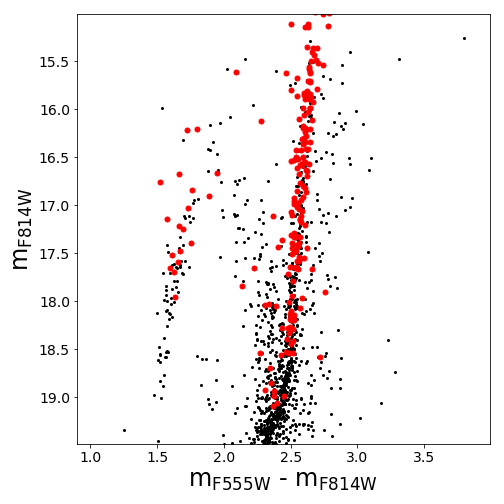
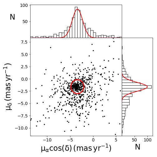
Figure 8: Left panel: Differential reddening-corrected CMD of NGC 6256 (same as in the right panel of Figure 1), showing only the stars in common with the Gaia DR2 catalog. The red dots correspond to the stars included within the red circle shown in the VPD in the right panel of the figure. Right panel: The main panel shows the VPD of the stars in common between our HST catalog and the Gaia DR2 catalog. The upper and side plots show the histograms of the proper motions along RA and Dec, with superimposed a best-fit Gaussian function. The red circle in the main panel is centered on the mean values of the best-fit Gaussian functions and has a radius of 1.4 mas yr^-1, equal to the combined $1\sigma$ values. This circle encloses all the stars that have been used to measure the cluster absolute PM.

5.3 The cluster orbit

The cluster absolute PM thus derived, combined with the radial systemic velocity from Vásquez et al. (2018, $v_{r}=-103.4\pm 0.5$ km s^-1), was used to back-integrate the cluster orbit within the Milky Way potential well. To this purpose, we used GravPot16 (Fernández-Trincado et al., 2017), a package that generates stellar orbits in a semi-analytic, steady-state and three-dimensional Galaxy model, based on the gravitational potential derived from the Besançon Galactic Model (Robin et al., 2003) and including also a prolate bar (Robin et al., 2012). This tool has been recently used to compute the orbits of several Galactic star clusters (Gaia Collaboration et al., 2018; Libralato et al., 2018; Bellazzini et al., 2019). The Galaxy parameters (such as the bar properties, Sun distance from the Galactic center, etc.) were set to the same standard values adopted by Gaia Collaboration et al. (2018). Figure 9 shows the resulting orbit of the cluster during the last Gyr. We verified that nothing significantly changes if the cluster initial conditions are randomly varied within the uncertainty ranges of its position and velocity. It can be seen that NGC 6256 is in a low-eccentricity orbit ($e\sim 0.11$), strongly confined within the Galactic bulge. In fact, during its $\sim 50$ Myr orbital period, it reaches a minimum and maximum distance from the Galactic center of about 0.8 kpc and 2.9 kpc, respectively. This confirms that, despite its relatively low metallicity, this system is not a halo intruder crossing the bulge during a fraction of its orbit (as suggested for other bulge GCs, like NGC 6681, Terzan 10 and Djorgovski 1, Massari et al., 2013; Ortolani et al., 2019a), but it is a GC genuinely belonging to the bulge population. As a consistency check, we compared our results with those obtained using different orbit integrators (see, e.g. Cadelano et al., 2017a) that adopt different shapes of the Galactic potential. We found that all the results are consistent within the uncertainties. These results are also qualitatively in agreement with those reported by Baumgardt et al. (2019). It is worth stressing that the simulated cluster orbit cannot be used to firmly asses if the cluster birthplace was indeed the Galactic bulge, since a back-integration of the orbit for a time as long as the cluster age should take into account the (basically unknown) variation of the Galactic potential as a function of time.

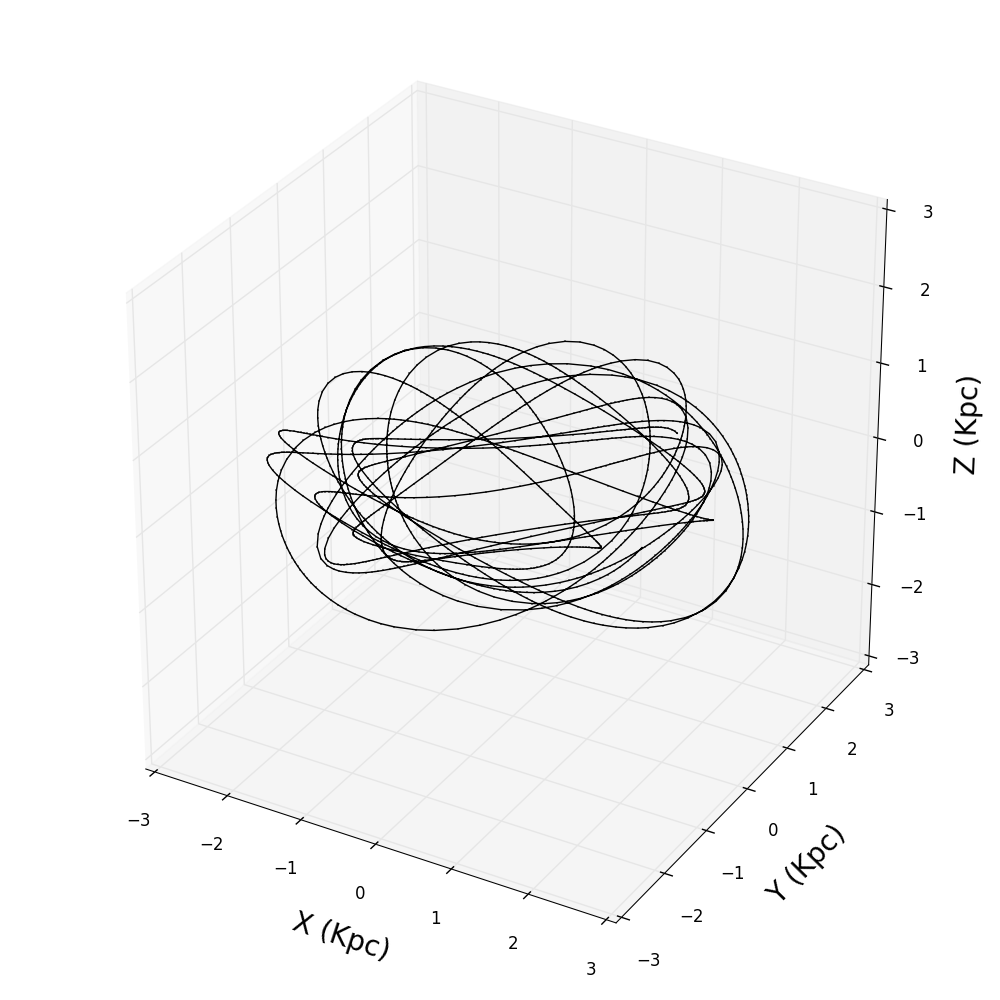
Figure 9: Simulated positions occupied by NGC 6256 in the last Gyr during its orbit within the Galaxy. The 3D axes cover a region smaller than the size of the Galactic bulge, thus confirming that the orbit of this cluster is well confined within it.

Massari et al. (2019) calculated the integrals of motion for a large sample of Galactic GCs to infer their birthplaces (i.e. to infer which clusters belong to the main Galactic population and which ones have been likely accreted during merger events that the Galaxy experienced in the past). To this aim they used the cluster current positions from Harris (2010) and kinematics from the Gaia DR2 catalog. They found that NGC 6256 is unlikely to belong to the Galaxy in situ population and it is most likely associated with an accreted low-energy component (see Figure 3 in Massari et al., 2019). However, their result is based on a distance value significantly different from the one computed here, while the cluster kinematic is in agreement with the results derived here and by Vásquez et al. (2018). We therefore repeated the same procedure followed by Massari et al. (2019) using the updated cluster position and found that NGC 6256 has a orbital energy of $E\sim-2.3\times 10^{5}$ km²/s² and an angular momentum of $L_{z}\sim-300$ km/s kpc. These updated values place NGC 6256 in a region of the integrals of motion space occupied by systems that genuinely belong to the population of bulge clusters formed in situ (Figure 10).

These dynamical arguments strongly suggest that NGC 6256 is an old and low-metallicity GCs that was formed in the bulge during the very early epoch of the Galaxy assembly.

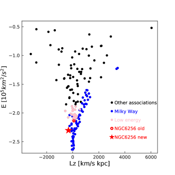
Figure 10: Integrals of motion for the sample of Galactic GCs analyzed in Massari et al. (2019). Blue points are clusters belonging to the Galaxy in situ population, pink points are those associated with an accreted low-energy component while black points are clusters with different associations. The position of NGC 6256 previously computed by Massari et al. (2019) is reported with a red open circle while its updated position is shown with a red star.

6 Summary and conclusions

We exploited, for the first time, deep and high resolution optical observations of the bulge globular cluster NGC 6256 to derive the main properties of its stellar population. The analysis revealed a population affected by high and differential reddening, which causes a severe blurring of all the cluster evolutionary sequences. We corrected the CMD position of each observed star for this effect and created a differential reddening map that reveals $E(B-V)$ variations up to $0.5$ mag across the $160\arcsec\times 160\arcsec$ field of view covered by the observations. In the differential reddening-corrected CMD, all the evolutionary sequences are nicely defined, and the main sequence is sampled down to 4 magnitudes below the turn-off. Our photometry confirmed that NGC 6256 is an outsider system with respect to most of the bulge GCs, since its stellar population is characterized by an extended and blue horizontal branch, suggesting a relatively low metal content, as confirmed by spectroscopic studies. These rare, relatively metal-poor GCs in the bulge are expected to be the oldest relics of the Galaxy assembly process and we thus performed isochrone fitting to determine the cluster stellar population age, along with other properties such as its distance and average color excess. It turned out that NGC 6256 is one of the oldest clusters known to date in the Galactic bulge. Indeed, the comparison with different sets of isochrones revealed a stellar population having an average age of $13.0$ Gyr with a typical uncertainty around $0.5$ Gyr. This result is particularly worth of attention: although bulge GCs are known to be 12 Gyr-old on average, improved age estimates are recently suggesting that metal-rich clusters are slightly younger (see the case of NGC 6528 in Lagioia et al. 2014; Calamida et al. 2014), while metal-poor GCs are preferentially older than this limit (NGC 6558, NGC 6522 and HP1; Barbuy et al. 2007; Kerber et al. 2018, 2019). The cluster age here obtained for NGC 6256 fits within such a scenario. We also found that NGC 6256 is affected by a large absolute color excess $E(B-V)=1.19$ and that its absolute distance modulus implies a distance of 6.8 kpc from the Sun. We finally determined the gravitational center and the absolute proper motion of the cluster, to then derive its orbit within a Galaxy-like potential. We found that NGC 6256 is moving in a low-eccentricity orbit entirely confined within the bulge, thus confirming that it is not a halo intruder crossing the bulge during its motion, but a genuine member of the Galactic bulge. Moreover, we computed the cluster integrals of motion and found that the cluster binding energy and angular momentum are compatible with those expected for a cluster purely belonging to the in situ Galactic bulge population. All together, these pieces of evidence indicate that NGC 6256 is one of the oldest systems formed within the bulge during the first stages of Galaxy assembly.

References

- Alcaino (1983) Alcaino, G. 1983, A&AS, 53, 47
- Allen & Santillan (1991) Allen, C., & Santillan, A. 1991, Rev. Mexicana Astron. Astrofis., 22, 255
- Arenou et al. (2018) Arenou, F., Luri, X., Babusiaux, C., et al. 2018, A&A, 616, A17
- Barbuy et al. (2007) Barbuy, B., Zoccali, M., Ortolani, S., et al. 2007, AJ, 134, 1613
- Baumgardt & Hilker (2018) Baumgardt, H., & Hilker, M. 2018, MNRAS, 478, 1520
- Baumgardt et al. (2019) Baumgardt, H., Hilker, M., Sollima, A., & Bellini, A. 2019, MNRAS, 482, 5138
- Bellini et al. (2011) Bellini, A., Anderson, J., & Bedin, L. R. 2011, PASP, 123, 622
- Bellazzini et al. (2019) Bellazzini, M., Ibata, R. A., Martin, N., et al. 2019, MNRAS, 2390
- Bica et al. (2016) Bica, E., Ortolani, S., & Barbuy, B. 2016, PASA, 33, e028
- Cadelano et al. (2017a) Cadelano, M., Dalessandro, E., Ferraro, F. R., et al. 2017, ApJ, 836, 170
- Cadelano et al. (2017b) Cadelano, M., Pallanca, C., Ferraro, F. R., et al. 2017, ApJ, 844, 53
- Cadelano et al. (2018) Cadelano, M., Ransom, S. M., Freire, P. C. C., et al. 2018, ApJ, 855, 125
- Cadelano et al. (2019) Cadelano, M., Ferraro, F. R., Istrate, A. G., et al. 2019, ApJ, 875, 25
- Calamida et al. (2014) Calamida, A., Bono, G., Lagioia, E. P., et al. 2014, A&A, 565, A8
- Cardelli et al. (1989) Cardelli, J. A., Clayton, G. C., & Mathis, J. S. 1989, ApJ, 345, 245
- Carretta et al. (2009) Carretta, E., Bragaglia, A., Gratton, R., et al. 2009, A&A, 508, 695
- Cescutti et al. (2008) Cescutti, G., Matteucci, F., Lanfranchi, G. A., et al. 2008, A&A, 491, 401
- Correnti et al. (2016) Correnti, M., Gennaro, M., Kalirai, J. S., Brown, T. M., & Calamida, A. 2016, ApJ, 823, 18
- Dalessandro et al. (2013) Dalessandro, E., Salaris, M., Ferraro, F. R., et al. 2013, MNRAS, 430, 459
- Dalessandro et al. (2018) Dalessandro, E., Lardo, C., Cadelano, M., et al. 2018, A&A, 618, A131
- Deustua et al. (2016) Deustua, S. E., Mack, J., Bowers, A. S., et al. 2016, Space Telescope WFC Instrument Science Report,
- Dotter et al. (2008) Dotter, A., Chaboyer, B., Jevremović, D., et al. 2008, ApJS, 178, 89-101
- Dotter et al. (2010) Dotter, A., Sarajedini, A., Anderson, J., et al. 2010, ApJ, 708, 698
- Fernández-Trincado et al. (2017) Fernández-Trincado, J. G., Robin, A. C., Moreno, E., et al. 2017, SF2A-2017: Proceedings of the Annual Meeting of the French Society of Astronomy and Astrophysics, Di
- Ferraro et al. (1999) Ferraro, F. R., Messineo, M., Fusi Pecci, F., et al. 1999, AJ, 118, 1738
- Ferraro et al. (2006) Ferraro, F. R., Valenti, E., & Origlia, L. 2006, ApJ, 649, 243
- Ferraro et al. (2009) Ferraro, F. R., Dalessandro, E., Mucciarelli, A., et al. 2009, Nature, 462, 483
- Ferraro et al. (2015) Ferraro, F. R., Pallanca, C., Lanzoni, B., et al. 2015, ApJ, 807, L1
- Ferraro et al. (2016) Ferraro, F. R., Massari, D., Dalessandro, E., et al. 2016, ApJ, 828, 75
- Foreman-Mackey et al. (2016) Foreman-Mackey, D., Vousden, W., Price-Whelan, A., et al. 2016, Zenodo Software Release, 2016
- Foreman-Mackey et al. (2019) Foreman-Mackey, D., Farr, W., Sinha, M., et al. 2019, The Journal of Open Source Software, 4, 1864
- Gaia Collaboration et al. (2016) Gaia Collaboration, Brown, A. G. A., Vallenari, A., et al. 2016, A&A, 595, A2
- Gaia Collaboration et al. (2018) Gaia Collaboration, Brown, A. G. A., Vallenari, A., et al. 2018, A&A, 616, A1
- Girardi et al. (2002) Girardi, L., Bertelli, G., Bressan, A., et al. 2002, A&A, 391, 195
- Gratton et al. (2003) Gratton, R. G., Bragaglia, A., Carretta, E., et al. 2003, A&A, 408, 529
- Harris (1996) Harris, W. E. 1996, AJ, 112, 1487
- Harris (2010) Harris, W. E. 2010, arXiv e-prints, arXiv:1012.3224
- Hockney & Eastwood (1988) Hockney, R. W., & Eastwood, J. W. 1988, Bristol: Hilger, 1988,
- Johnson & Soderblom (1987) Johnson, D. R. H., & Soderblom, D. R. 1987, AJ, 93, 864
- Kerber et al. (2018) Kerber, L. O., Nardiello, D., Ortolani, S., et al. 2018, ApJ, 853, 15
- Kerber et al. (2019) Kerber, L. O., Libralato, M., Souza, S. O., et al. 2019, MNRAS
- Lagioia et al. (2014) Lagioia, E. P., Milone, A. P., Stetson, P. B., et al. 2014, ApJ, 782, 50
- Lanzoni et al. (2007) Lanzoni, B., Dalessandro, E., Ferraro, F. R., et al. 2007, ApJ, 668, L139
- Lanzoni et al. (2010) Lanzoni, B., Ferraro, F. R., Dalessandro, E., et al. 2010, ApJ, 717, 653
- Lanzoni et al. (2019) Lanzoni, B., Ferraro, F. R., Dalessandro, E., et al. 2019, ApJ, 887, 176
- Libralato et al. (2018) Libralato, M., Bellini, A., Bedin, L. R., et al. 2018, ApJ, 854, 45
- Massari et al. (2012) Massari, D., Mucciarelli, A., Dalessandro, E., et al. 2012, ApJ, 755, L32
- Massari et al. (2013) Massari, D., Bellini, A., Ferraro, F. R., et al. 2013, ApJ, 779, 81
- Massari et al. (2014a) Massari, D., Mucciarelli, A., Ferraro, F. R., et al. 2014, ApJ, 795, 22
- Massari et al. (2014b) Massari, D., Mucciarelli, A., Ferraro, F. R., et al. 2014, ApJ, 791, 101
- Massari et al. (2015) Massari, D., Dalessandro, E., Ferraro, F. R., et al. 2015, ApJ, 810, 69
- Massari et al. (2019) Massari, D., Koppelman, H. H., & Helmi, A. 2019, A&A, 630, L4
- Milone et al. (2012) Milone, A. P., Piotto, G., Bedin, L. R., et al. 2012, A&A, 540, A16
- Milone et al. (2018) Milone, A. P., Marino, A. F., Renzini, A., et al. 2018, MNRAS, 481, 5098
- Moffat (1969) Moffat, A. F. J. 1969, A&A, 3, 455
- Montegriffo et al. (1995) Montegriffo, P., Ferraro, F. R., Fusi Pecci, F., & Origlia, L. 1995, MNRAS, 276, 739
- Origlia et al. (2011) Origlia, L., Rich, R. M., Ferraro, F. R., et al. 2011, ApJ, 726, L20
- Origlia et al. (2013) Origlia, L., Massari, D., Rich, R. M., et al. 2013, ApJ, 779, L5
- Origlia et al. (2019) Origlia, L., Mucciarelli, A., Fiorentino, G., et al. 2019, ApJ, 871, 114
- Ortolani et al. (1999) Ortolani, S., Barbuy, B., & Bica, E. 1999, A&AS, 136, 237
- Ortolani et al. (2011) Ortolani, S., Barbuy, B., Momany, Y., et al. 2011, ApJ, 737, 31
- Ortolani et al. (2019a) Ortolani, S., Nardiello, D., Pérez-Villegas, A., et al. 2019, A&A, 622, A94
- Ortolani et al. (2019b) Ortolani, S., Held, E. V., Nardiello, D., et al. 2019, A&A, 627, A145
- Pallanca et al. (2019) Pallanca, C., Ferraro, F. R., Lanzoni, B., et al. 2019, ApJ, 882, 159
- Pietrinferni et al. (2004) Pietrinferni, A., Cassisi, S., Salaris, M., et al. 2004, ApJ, 612, 168
- Pietrinferni et al. (2006) Pietrinferni, A., Cassisi, S., Salaris, M., et al. 2006, ApJ, 642, 797
- Piotto et al. (2002) Piotto, G., King, I. R., Djorgovski, S. G., et al. 2002, A&A, 391, 945
- Pryor & Meylan (1993) Pryor, C., & Meylan, G. 1993, Structure and Dynamics of Globular Clusters, 50, 357
- Reid et al. (2009) Reid, M. J., Menten, K. M., Zheng, X. W., et al. 2009, ApJ, 700, 137-148
- Robin et al. (2003) Robin, A. C., Reylé, C., Derrière, S., et al. 2003, A&A, 409, 523
- Robin et al. (2012) Robin, A. C., Marshall, D. J., Schultheis, M., et al. 2012, A&A, 538, A106
- Saracino et al. (2015) Saracino, S., Dalessandro, E., Ferraro, F. R., et al. 2015, ApJ, 806, 152
- Saracino et al. (2016) Saracino, S., Dalessandro, E., Ferraro, F. R., et al. 2016, ApJ, 832, 48
- Saracino et al. (2019) Saracino, S., Dalessandro, E., Ferraro, F. R., et al. 2019, ApJ, 874, 86
- Sarajedini et al. (2007) Sarajedini, A., Bedin, L. R., Chaboyer, B., et al. 2007, AJ, 133, 1658
- Schlafly, & Finkbeiner (2011) Schlafly, E. F., & Finkbeiner, D. P. 2011, ApJ, 737, 103
- Schönrich et al. (2010) Schönrich, R., Binney, J., & Dehnen, W. 2010, MNRAS, 403, 1829
- Stephens & Frogel (2004) Stephens, A. W., & Frogel, J. A. 2004, AJ, 127, 925
- Stetson (1987) Stetson, P. B. 1987, PASP, 99, 191
- Stetson (1994) Stetson, P. B. 1994, PASP, 106, 250
- Valenti et al. (2007) Valenti, E., Ferraro, F. R., & Origlia, L. 2007, AJ, 133, 1287
- VandenBerg et al. (2014) VandenBerg, D. A., Bergbusch, P. A., Ferguson, J. W., & Edvardsson, B. 2014, ApJ, 794, 72
- Vasiliev (2019) Vasiliev, E. 2019, MNRAS, 484, 2832
- Vásquez et al. (2018) Vásquez, S., Saviane, I., Held, E. V., et al. 2018, A&A, 619, A13
- Walker et al. (2006) Walker, M. G., Mateo, M., Olszewski, E. W., et al. 2006, AJ, 131, 2114
- Webbink (1985) Webbink, R. F. 1985, Dynamics of Star Clusters, 541