Time sequence spectroscopy of Epsilon CrA.
The 518 nm Mg I triplet region analyzed with Broadening Functions

Abstract

High-resolution spectroscopic observations of the W UMa-type binary $\epsilon\,$CrA obtained as a time monitoring sequence on four full and four partial nights within two weeks have been used to derive orbital elements of the system and discuss the validity of the Lucy model for description of the radial-velocity data. The observations had more extensive temporal coverage and better quality than similar time-sequence observations of the contact binary AW UMa. The two binaries share several physical properties with both showing very similar deviations from the Lucy model: The primary component is a rapidly-rotating star almost unaffected by the presence of the secondary component, while the latter is embedded in a complex gas flow and appears to have its own rotation-velocity field, in contradiction to the model. The spectroscopic mass ratio is found to be larger than the one derived from the light-curve analysis, similarly as in many other W UMa-type binaries, but the discrepancy for $\epsilon\,$CrA is relatively minor, much smaller than for AW UMa. The presence of the complex velocity flows contradicting the solid-body rotation assumption suggest a necessity of modification to the Lucy model, possibly along the lines outlined by Stȩpień (2009) in his concept of the energy transfer between the binary components.

1 Introduction

$\epsilon\,$Coronae Austrinae (Epsilon CrA, hereinafter $\epsilon\,$CrA; HD 175813, HR 7152, F2V, $V=4.8$, $B-V=0.36$, $P=0.591$ d.) is the brightest known binary star of the W UMa type. Such stars are also frequently called “contact binaries” because they achieve a state of physical equilibrium in actual physical contact permitting free exchange of energy between their components. The result is the observed equality of the effective temperature over the whole binary structure. Since the component masses always differ, with typical mass ratios around 0.3 to 0.5 and the steep mass-luminosity relations, the more massive component provides practically all luminous energy while the less massive component carries the angular momentum of the binary and contributes its radiation area to the combined system luminosity. The first physically acceptable structure model of the W UMa binaries was developed by Lucy (1968a). The companion study, Lucy (1968b), used its assumptions to give a prescription on light-curve models utilizing the Roche-model equipotentials. While the light-curve model enjoys immense popularity with hundreds or thousands of light curves synthesized so far, the large body of observational results has not resulted in much progress in the understanding of the energy exchange process which is so crucial for the structure model. A vigorous and often heated discussion of the 1970’s died out when it was realized that most severe controversies cannot be resolved using physical arguments without observational support. As a result, the structure model of Lucy (1968a) is assumed valid irrespective of the energy transfer processes operating in these binaries. We return to this important subject at the end of the paper, in Section 4.2, in a discussion of structure and energy transport models.

The current study has been motivated by the similarity $\epsilon\,$CrA to AW UMa, the first and currently the only contact binary which has been studied spectroscopically in sufficient detail using the high-resolution, continuous, time-monitoring observations (Rucinski, 2015, Paper I). Both binaries have small mass ratios close to 0.1. It is not clear if rather moderate numbers of known such small mass-ratio W UMa binaries is an observational selection bias or a genuine property of the group; extensive sky surveys will soon resolve this matter. We assume that both binaries are contact binaries with the same processes operating in them as in more common systems with mass ratios around 0.3 – 0.5. The results for AW UMa were surprising and in discord with the Lucy model: the binary turned out to be a puzzling case of a binary which observed photometrically – and analyzed for the light-curve variations – seemed to be a perfect illustration of the Lucy model, and yet – spectroscopically – appeared to resemble a semi-detached binary with the primary losing its matter and engulfing the secondary in its outer layers. The current observations and analysis of $\epsilon\,$CrA were meant as an attempt to answer the question: Is AW UMa an atypical binary? Or, more importantly, is the dichotomy in the photometry versus spectroscopy telling us that photometry does not carry sufficient information through its spectrum-integrating nature? In other words, is bringing one more dimension into the temporal analysis necessary to see the full complexity of such a binary system?

Radial velocities are easy to predict with the Lucy model (Rucinski, 2012). The model envisages the two stellar components filling the same common Roche-model equipotential and rotating as a solid body with a total absence of velocities in the rotating system of coordinates. Extensive use of the model for the moderate spectral resolution observations of 90 W UMa binaries at the David Dunlap Observatory (a very brief summary is in Rucinski (2013, Sec. 2)) appeared to confirm the model. However, the high-resolution, high-quality data presented in Paper I showed that AW UMa contradicts the Lucy model and indicated a need for its modifications. The essential results of Paper I (see also the earlier work on AW UMa by Pribulla & Rucinski (2008)) are as follows:
1. The upper 70% of the rotational profile of the rapidly-rotating primary of AW UMa agrees with that of a single star unaffected by the presence of its companion and rotating at the projected equatorial velocity $V\sin i$ of about 85% of the orbital synchronism.
2. An additional, high rotation-rate velocity component called “the pedestal” extends the profile width to that expected for the rotating Roche-model structure.
3. The surface of the primary component is covered by more regularly distributed “ripples” and relatively isolated “spots”. These features may be located at different stellar latitudes with different rotation rates, as indicated by different rates of migration across the stellar profile.
4. The secondary component possesses a velocity field embedded in the inter-binary gas flow. Its flat or meniscus-shaped rotation profile does not show a central condensation, suggesting a detached star of unusual velocity distribution rather than a component of the Lucy model.
5. In spite of the velocity field modified by the inter-binary flows, the phase dependence of the integrated spectral-line intensities (integrated equivalent widths) (Paper I, Fig. 2) roughly agrees with the photometric data. The variations can be explained by making a simple assumption of a phase-invariable primary with all equivalent-line-width phase variations due to changing visibility of the secondary component and of its surrounding matter.
6. The masses of the two components of AW UMa are: $M_{1}\sin^{3}i=1.29\pm 0.15\,M_{\odot}$, $M_{2}\sin^{3}i=0.128\pm 0.016\,M_{\odot}$ (for the assumed $i\simeq 80^{0}$ as for the Lucy model). Irrespectively of the model, the orbital inclination is not far from the edge-on orientation so that the above minimum-mass estimates are close to the actual ones. The spectroscopic mass ratio, $q_{\rm sp}=0.10$, is different from the indicated by photometric results using the Lucy model, $q_{\rm ph}=0.08$, with the formal uncertainties of both methods several tens-of-times smaller than their difference.
7. The moderate period change of AW UMa of $dP/dt=-5.3\times 10^{-10}$ (Rucinski et al., 2013) could be interpreted by a net mass-transfer from the primary to the secondary at a rate of about $dM/dt\simeq-2\times 10^{-8}M_{\odot}/{\rm yr}$.

Paper I, although presenting unexpected results for AW UMa, has gone critically uncommented except for the important investigation by Eaton (2016) who carefully considered possible ways of reconciling the new spectroscopic results with the Lucy light curve model. Several of the suggested modifications (e.g. large photospheric spots) would imply the introduction of many arbitrary parameters just to fit the data, but some criticism may be valid (e.g.  the use of the flux spectrum as a template in view of the complex geometry of the local light emergence).

The observations of $\epsilon\,$CrA reported in this paper required extensive use of a very stable, high-resolution spectrograph on a moderate-size telescope. Such observations are not easy to arrange and execute. Because of the high brightness of the star and several and some organizational reasons, it turned out easier to arrange a continuous spectral time-monitoring for $\epsilon\,$CrA than for V566 Oph for which we had important indications from lower-resolution work (Pribulla & Rucinski, 2008; Rucinski, 2010) that the Lucy model may work correctly. Thus, instead of attempting to analyze an object entirely different from AW UMa, we concentrated on the uniqueness of that binary and on general lessons for the most appropriate model of W UMa binaries.

Although $\epsilon\,$CrA with $V=4.8$ is a relatively bright star, the previous analyses on $\epsilon\,$CrA have not been extensive. The early light-curve studies of Knipe (1967) and Tapia (1969) have remained the main photometric source for the Lucy model light-curve studies of Twigg (1979) and, especially Wilson & Raichur (2011), who pushed the Lucy model to its full, extensive consequences with many parameters determined at the same time. The orbital inclinations were determined to be $i=72.24\pm 0.50$ degrees (Twigg, 1979) and $i=73.05\pm 0.16$ degrees (Wilson & Raichur, 2011), both consistently smaller than the orbital inclination of AW UMa estimated at $i\simeq 78-80$ degrees (see Paper I). The photographic line-by-line radial-velocity analysis by Tapia & Whelan (1975) was substantially improved by the study of Goecking & Duerbeck (1993) who detected the secondary component using the cross-correlation function (CCF) technique, finding the mass ratio of $q_{\rm sp}=0.128\pm 0.014$. This mass ratio is significantly larger than the formally very accurate photometric results of Twigg (1979), $q_{\rm ph}=0.114\pm 0.003$ and Wilson & Raichur (2011), $q_{\rm ph}=0.1244\pm 0.0014$. The study by Goecking & Duerbeck (1993) was the closest in spirit to the current one as our Broadening-Functions technique can be considered an improvement on the CCF, but based on a linear transformation rather than a non-linear one (Rucinski, 2002) and retaining the full spectral resolution of the data. The reader is advised to consult Paper I as the current paper is very closely related to the AW UMa study (Rucinski, 2015).

The $\epsilon\,$CrA spatial velocity does not differ appreciably in its general properties from the majority of the nearby W UMa binaries (Rucinski, 2013) which appear to be galactic-disk, kinematically-old objects. With the assumed: $\mu_{\rm RA}=-132.2\pm 0.41$ mas/yr, $\mu_{\rm Dec}=-98.4\pm 0.38$ mas/yr and $\pi=32.01\pm 0.27$ mas (Gaia Collaboration, 2016, 2018) and our new $V_{0}=62.541$ km s^-1 (Section 3.2 and Table 4), the spatial velocity components are $U=+71.9$, $V=-7.8$ and $W=+0.2$, all in km s^-1, with the convention on the $U$ vector direction as in Rucinski (2013). The tangential velocities are moderate and it is only the radial direction in which the space-velocity vector is larger. The absolute magnitude $M_{V}=+2.3$ implies a relatively bright star for its spectral type. In addition to the most frequently cited F2V, the spectral type of $\epsilon\,$CrA was estimated by Grey et al. (2006) to be as late as F4VFe-0.8. Both, the high luminosity and the slightly later spectral type than of AW UMa suggest a binary object with stellar cores somewhat advanced in their evolution.

The paper presents the observations of $\epsilon\,$CrA in Section 2 and their results in Section 3. The new results and those for AW UMa suggest a re-discussion of the venerable Lucy model. The essential directions for such an effort in view of the results for both binaries are outlined in Conclusions in Section 4.

2 Observations and their processing

Observations of $\epsilon\,$CrA were made in the service mode with the CHIRON spectrograph (Tokovinin et al., 2013) on the CTIO/SMARTS 1.5m telescope on eight nights between 12 to 29 July 2018. Six nights were within the first week while the remaining two were two weeks later (see Table 1). The first three nights were clear, but the following nights were affected to a various degree by the variable weather conditions of the Chilean winter. The overall span of the $\epsilon\,$CrA observations of 17 days is much longer than for AW UMa for which all observations were collected in three consecutive nights. Altogether, 361 exposures of 450 seconds were taken using the slicer setup which provides a spectral resolving power of $R=80,000$. An attempt was made to retain the same time resolution throughout the program. The median spacing between the observations was 468 seconds or 7.8 minutes which is a less rapid data-taking rate than used for AW UMa where the median cadence was 2.1 minutes. The longer exposures and more observation nights resulted in the total amount of exposure time for $\epsilon\,$CrA of 2705 minutes; this should be compared with 876 minutes for AW UMa.

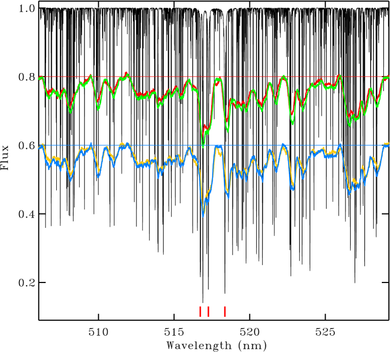
Figure 1: The model-spectrum template used for the Broadening-Functions deconvolution technique (thin black line) and the observed spectra of $\epsilon\,$CrA (in color) are shown together, with the observed spectra shifted by $-0.2$ for the orbital phases 0.25 and 0.5 (red and green lines) and $-0.4$ for the phases 0.75 and 0.0 (orange and blue lines), respectively. The spectral region is centered on the Mg I “b” triplet. The integrated spectral-line absorption in the whole spectral window is 5.51 percent and is due mostly to iron lines with the magnesium triplet contributing 0.64 percent to that number. The lines of the triplet are marked by the red bars at the bottom part of the figure.

Table 1: Observing nights of $\epsilon\,$CrA

July 2018	$HJD$	$Orb$	$N$
12	58312.5211 – 58312.8785	0.7601 – 1.3643	66
13	58313.5402 – 58313.8870	2.4830 – 3.0693	64
14	58314.5356 – 58314.8600	4.1660 – 4.7145	60
15	58315.5380 – 58315.5631	5.8608 – 5.9033	6
16	58316.5378 – 58316.8031	7.5513 – 7.9998	49
18	58318.6736 – 58318.8660	11.1622 – 11.4876	36
26	58326.5976 – 58326.7576	24.5597 – 24.8304	30
28	58328.5632 – 58328.8552	27.8830 – 28.3768	54

Note. — The mid-exposure time ranges for individual nights are expressed as $HJD-2,400,000$. $Orb$ gives the range in time in units of the orbital period, continuously counted from the assumed initial epoch $HJD=2\,458\,312.0716$ and $P=0.59145447$ day; the fractional part of $Orb$ is the orbital phase. $N$ is the number of star spectra obtained on a given night. The nights are identified by the day in July 2018.

The spectral region used for $\epsilon\,$CrA was 506.05 nm to 529.20 nm, which is slightly wider at the short-wavelengths than the region adopted for AW UMa additionally contributing to improved final results. The spectral sampling at the conversion step from wavelengths to velocities was set at 1.8 km s^-1 leading to 7450 points in the utilized spectrum. Four typical spectra for the cardinal orbital phases of the binary are shown in Figure 1 together with the spectrum of the template used for the Broadening-Functions (BF) processing. The spectra are dominated by the strong rotational broadening at all orbital phases. The orbital-phase variations – the subject of this paper – are rather subtle, mostly masked by strong overlapping of the broadened lines. This stresses the necessity of high quality data and of an efficient information-extraction technique. The Broadening-Functions technique in the most convenient as it derives information on the velocity field using a linear deconvolution of the rotation- and orbital motion-broadened spectrum. The final product is a function similar to a cross-correlation, but having an important advantage of linearity and thus of a direct mapping of the radial velocity field into the spectral wavelength domain. The function integral is normalized to unity for a perfect match of the integrated equivalent width of the spectral lines to that of the template spectrum. The function recovers the actual level of the spectral continuum which is not accessible in the wavelength domain.

Parameters of the BF processing of the $\epsilon\,$CrA data were set at the same values as for the case of AW UMa, as described in Paper I. Similarly, the spectra were smoothed to the effective resolution characterized by a Gaussian with the FWHM of 8.5 km s^-1, corresponding to the resolving power $R\simeq 35,000$. The Broadening-Functions (BF) processing was used to determine the functions at 551 points leading to the strong, 13.5-fold over-determinacy of the final, individual profiles. As the template, we used the same model-atmosphere flux spectrum of a F2V star, calculated by Dr. Jano Budaj for AW UMa. Because of the very wide spectral lines and the atypical appearance of the spectrum, the spectral type of $\epsilon\,$CrA has been estimated in the literature as ranging between F0V and F4V; the color index $B-V=0.36$ agrees with F2V (for AW UMa: $B-V=0.33$). The BF’s calculated for the available spectra of $\epsilon\,$CrA are characterized by a median $S/N\simeq 120$. Thus, they are substantially more accurate than those for AW UMa ($S/N\simeq 57$) reflecting the longer exposures and the higher apparent brightness of $\epsilon\,$CrA. The BF’s are listed in Table 2. The overall size of the table is almost $2\!\times\!10^{5}$ numbers stored in a compact, integer form; storage of the spectra would take 13.5 times more space.

A prediction of the moment of primary (deeper) eclipses of the more-massive star by the secondary component, based on photometric data have been provided to the author by Prof. J. Kreiner and Dr. B. Zakrzewski of Cracow. The data covered the years 1960 to 2017 so that the ephemeris required extrapolation forward in time. The quadratic ephemeris is: $HJD=2\,439\,707.6624(2)+0.59143046(23)\times E+3.817(79)\,10^{-10}\times E^{2}$, with the uncertainties of the last digits given in parentheses. For an eclipse occurring just before the start of our observations, the epoch and time are: $E=41456$, $HJD=2\,458\,312.0766$. A sine fit to the radial velocities of the primary component of $\epsilon\,$CrA (see Section 3.1) ) gave a slightly different value for the mid-primary eclipse which has been adopted as the origin for our orbital-phase reckoning. The final, locally-linear prediction for the primary eclipses that we used was: $HJD=2\,458\,312.0716+0.59145447\times E_{1}$, with $E_{1}=1$ for the first of the observed eclipses.

A continuous measure of time, but expressed in the orbital period as a unit, is a convenient argument to see changes taking place in AW UMa over a few orbital cycles. We use the same quantity for $\epsilon\,$CrA, equivalent to $E_{1}$ above, but expressed as a real number with its fractional part being the familiar orbital phase called hereinafter $\phi$; we call it the “orbit” ($Orb$). Our data covered the orbits $0.760\leq Orb\leq 28.377$.

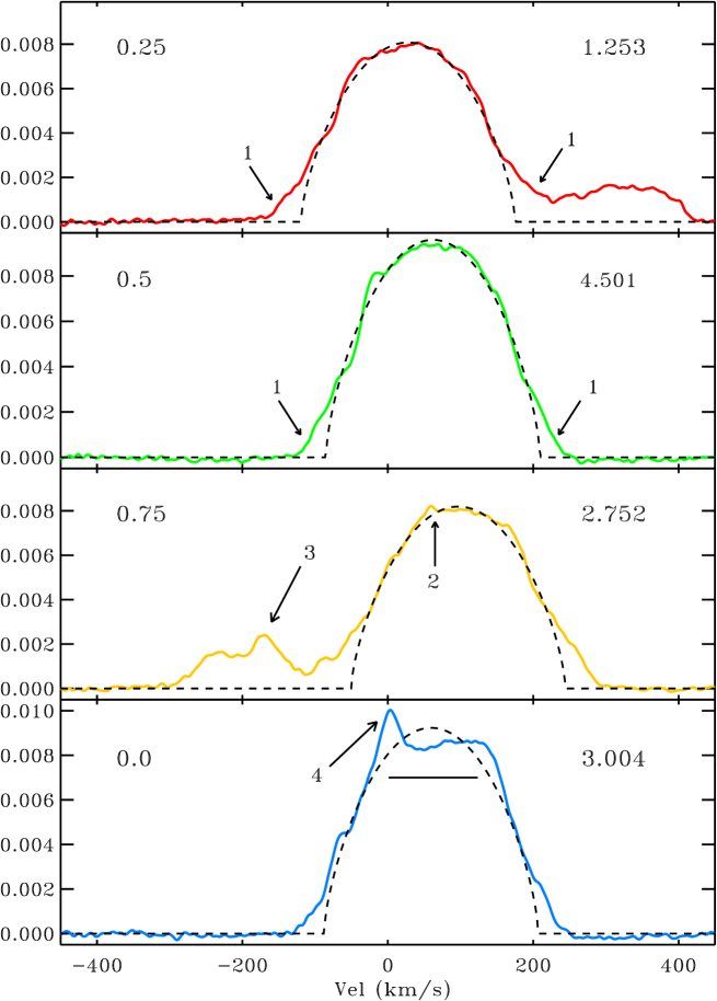
Figure 2: Broadening Functions (BF) for four observations close to orbital quadratures and mid-eclipses with the color coding corresponding to that used in Figure 1. The nominal orbital phases are given in the left upper corners of the panels while the orbits ($Orb$, see the text) of the actual observations are in the right upper corners. The units of the vertical scale relate to the normalization of the BF integrals to the template when sampled at 1.8 km s^-1 (unity for the exact spectral match of the spectra). The BF features indicated by the numbers are: 1 – the pedestal; 2 – a surface inhomogeneity; 3 – the “wisp”, a radial-velocity structure associated with the secondary component of the binary (Section 3.3); 4 – the flow of matter over the surface of the secondary component directed toward the observer (Section 3.1). The broken lines give the vertically-scaled rotational profile for $V\sin i=147$ km s^-1. In the lowest panel, the horizontal bar shows the expected velocity extent ($\pm 64$ km s^-1) of a Lucy-model, synchronously-rotating secondary component with $q=0.13$, for $i=73$ degrees; the secondary is filling the inner critical common equipotential passing through the $L_{1}$ point, see Section 3.2 and Table 5.

3 The results

3.1 The primary component

The Broadening Functions (BFs) for $\epsilon\,$CrA are very similar to those of AW UMa in that they are dominated by the strong feature of the primary component of the binary system. We show the BFs for four cardinal orbital phases in Figure 2; the results for other observations are tabulated in Table 2. We see that: (1) The rotational profile of single, rapidly rotating star with $V\sin i=147$ km s^-1 describes the upper part of the primary component profile (above the 0.35 of the maximum) very well; the transit eclipse being an obvious exception; (2) The profile shows high-velocity extension wings which we called the “pedestal” for the case of AW UMa; (3) The primary component surface appears to be covered by low-contrast inhomogeneities to a lesser degree than in AW UMa, and (4) Obvious signs of distributed matter in the binary are present and may be affecting the primary profile. One of such is a conspicuous BF perturbation at the primary (deeper) eclipse during the transit of the secondary over the disk of the primary component (the lowest panel in Figure 2). The perturbation, in the form of a spike is most likely caused by gaseous matter flowing towards the observer over the surface of the secondary component; this is discussed further in Section 3.2.

Table 2: Broadening Functions

	-4950	-4932	-4914	-4896	-4878	-4860	…
5211	-336	-159	-39	19	9	-46	…
5263	-330	-202	-137	-99	-63	-25	…
5319	-289	-113	-4	41	27	-32	…
5372	-419	-256	-145	-64	-8	19	…
5426	-313	-167	-80	-29	-3	-6	…
…

Note. — The table has 361 rows of 551 numbers corresponding to the number of observations and the length of the BF functions. For efficient transfer, the ASCII file has all numbers scaled and converted to integers. The first row gives 551 radial velocities in the heliocentric system, expressed in km s^-1 and multiplied by 10 (format: 6x,551i6). The subsequent 361 rows (format: 552i6) give, in the first position, the time $T=HJD-2\,458\,312$ multiplied by $10^{4}$, and then 551 values of the Broadening Function multiplied by $10^{6}$. Thus, the velocities in the first row are: $-495.0$, $-493.2$, $-491.4$, $-489.6$, $-487.8$, $-486.0$, … km s^-1 and the corresponding BF values at $T=0.5211$ are: $-0.000336$, $-0.000159$, $-0.000039$, $0.000019$, $0.000009$, $-0.000046$.

This table is available in the on-line version only.

The details in the profiles in Figure 2 are all significant and are not caused by the BF uncertainties which are very small (Section 2). The errors have a constant distribution along the whole length of a given BF; their size may be estimated directly from the scatter in the baseline, for example from the empty portion at velocities $<350$ km s^-1. It is one of the advantages of the BF approach that all points are treated equivalently and independently by the linear deconvolution process. The spectral resolution of FWHM of 8.5 km s^-1 was set at the start of the BF determination and is the only source of correlation between the data points.

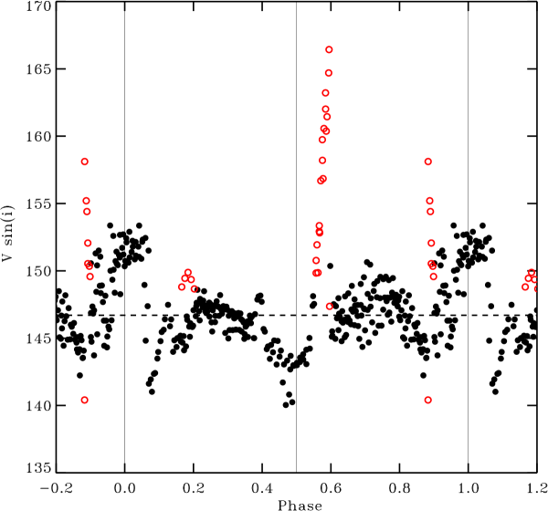
Figure 3: The projected equatorial velocity $V\sin i$ of the primary component of $\epsilon\,$CrA determined by rotation-profile fits to individual Broadening Functions. The figure shows the results of the fits to the upper 65% of the primary-component profile. The data strongly affected by the distributed matter in the system and not used for the primary radial-velocity orbit are marked by red, open circles. The horizontal broken line gives the adopted value of $V\sin i=147$ km s^-1.

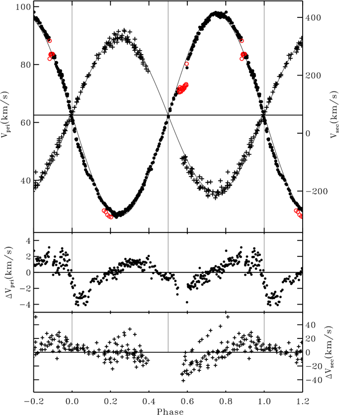
Figure 4: The radial velocity orbit of $\epsilon\,$CrA. The primary component velocities (circles and the left vertical axis) were determined by rotational-profile fits to the upper 65% of the primary BF feature. The data not used in the sine-curve fit are marked by red, open circles. The secondary component velocities (crosses, the right axis compressed by 10-times in scale relative to the left axis) were determined as profile centroids in 2D images formed from the BF functions, such as Figures 5–9. The two lower panels show the velocity residuals, with different scales for the primary and secondary components.

The width of the primary component profile (Figure 3) changes slightly with the orbital phase. The solid-body rotational profile for the limb darkening coefficient $u=0.5$ was fit to the individual profiles above 0.35 of the maximum value to avoid contamination by the high-velocity pedestal. The fits gave the smallest $V\sin i\simeq 143$ km s^-1 during the short interval of the secondary (shallower) eclipse, $\phi=0.5$, when the secondary component with all its complications (Sections 3.2–3.3) underwent the occultation by the primary. This interval appears to be longer before the center of the eclipse, starting $\phi\simeq 0.40$ and ends abruptly $\phi\simeq 0.54$. These phases coincide with large perturbations of the primary profile by an unexplained spectral feature discussed further in Section 3.3. The short duration of the totality phases agrees with the orbital inclination angle of $i\simeq 72-73$ degrees (Twigg, 1979; Wilson & Raichur, 2011) estimated from the approximate relations of Mochnacki & Doughty (1972) and our determination of the mass ratio of $q_{\rm sp}=0.13$ (Section 3.2). The median projected equatorial velocity for all phases is $V\sin i=147\pm 3$ km s^-1, where the assigned uncertainty is an estimate of the scatter at orbital phases away from the extended wings of the eclipses and not perturbed by the gas streams (Figure 2). Of the total of 361 observations, 32 rotational-profile fits were noticeably disturbed by optically-thick gas motions in the system and were eliminated from the determination of the primary component orbit (marked by red open circles in Figure 3). The rotation rate of $V\sin i=147$ km s^-1 is about 80–85% of the rotation synchronous with the orbital motion of the inner critical equipotential ($178\,\sin i$ km s^-1); however, the additional broadening in the pedestal of about 25 – 35 km s^-1 would bring it into an approximate agreement with the synchronous rate.

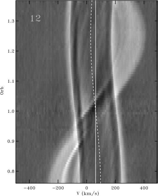
Figure 5: The two-dimensional representation of the BF temporal variability during the night #12; the nights of our program are numbered by the days of July 2018. The scaled and orbital-velocity shifted rotational-profile fits to the primary component profile, with the assumed $V\sin i=147$ km s^-1, have been subtracted to reduce the dynamic range of the image. The horizontal scale gives the heliocentric velocity while the vertical scale running upwards gives the time expressed in $Orb$ units; the fractional part of the $Orb$ is the familiar orbital phase counted from the deeper (transit) eclipse. The vertical white line gives the velocity of the mass center while the broken line gives the fit to the centroid of the primary component. The two bright bands along the residual profile of the primary component show the pedestal, a feature marked in Figure 2 by the label 1. The enhanced, approaching side of the secondary component is interpreted as a stream of matter over its surface during the transit eclipse ($orb=1$).

Table 3: The radial velocities of the primary component of $\epsilon\,$CrA

$HJD$	$Orb$	$V_{1}$	$V\,\sin i$	Key
0.5211	0.760	97.84	149.6	1
0.5263	0.769	97.07	149.3	1
0.5319	0.778	97.07	148.4	1
0.5372	0.787	96.59	147.9	1
0.5426	0.796	96.63	147.8	1

Note. — The columns are as follows:

$HJD$ – the heliocentric JD for the middle of the exposure counted from $HJD=2458312$;

$Orb$ – the same time expressed with the orbital period as an unit;

$V_{1}$ – the centroid of the rotational velocity fitting profile expressed in km s^-1;

$V\,\sin i$ – the projected rotational velocity determined from the upper 65 precent of the profile;

$Key$ – zero signifies that the observation was not used for the primary-component velocity determination.

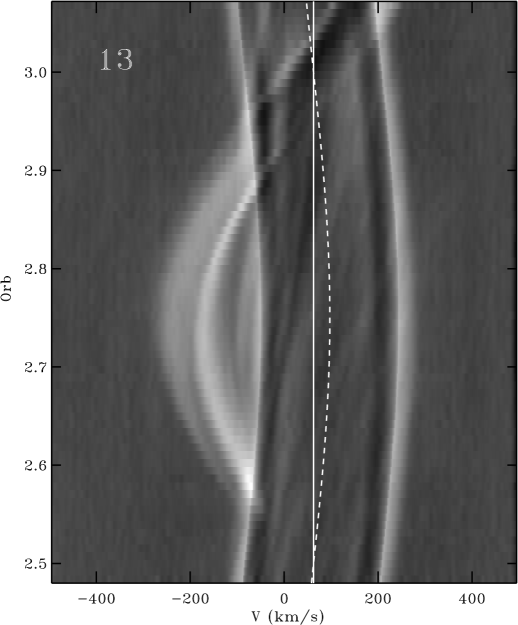
Figure 6: The same as in Figure 5 for 13 July 2018 when the secondary component was approaching us during the orbital quadrature. Note the complex structure of the secondary component for the orbital phases centered at $\phi\simeq 0.75$. The most prominent feature is called the “wisp”; it is marked by label 3 in Figure 2. In may represent a stationary spot in the volume between the stars.

The radial-velocities of the primary component of $\epsilon\,$CrA are listed in Table 3 while the orbital solution based on the centroids of the rotational-profile fits is shown in Figure 4. The orbital fit to these velocities by a sine curve is very well defined, particularly after the strongly deviating measurements close to the phases around 0.58 and 0.87 are removed. The zero point determined here is used in this paper as the origin of the orbit and orbital-phase counting. The resulting parameters of the spectroscopic orbit for the primary component are listed in Table 4, together with the results for the secondary component discussed in the next Section 3.2. The orbital period $P$ is for the locally linear ephemeris following the quadratic elements in Section 2.

While the parameters of the sine-curve fit to the primary component radial velocities have very small errors, the quality of the fit is characterized by a relatively large single-point random error of $\pm 1.44$ km s^-1. As shown in Figure 4, the large fraction of the uncertainty is due to the systematic deviations reaching $-4$ to $+2$ km s^-1 close to the eclipses; the scatter at the orbital phases around 0.25 and 0.75 is considerably smaller, $\pm 0.38$ km s^-1. The deviations before and after the primary eclipse (the transit of the secondary component in front of the primary) are reminiscent of the “Rossiter–McLaughlin effect” effect which was also noticeable in the AW UMa velocity data. However, observed with the accuracy available here, the effect is not symmetric relative to the eclipse center implying the existence of gas-flow motions affecting even the central parts of the primary profile.

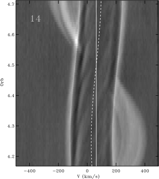
Figure 7: The same as in Figure 5 for the night of 14 July 2018, centered at the shallower eclipse, the secondary-component occultation.

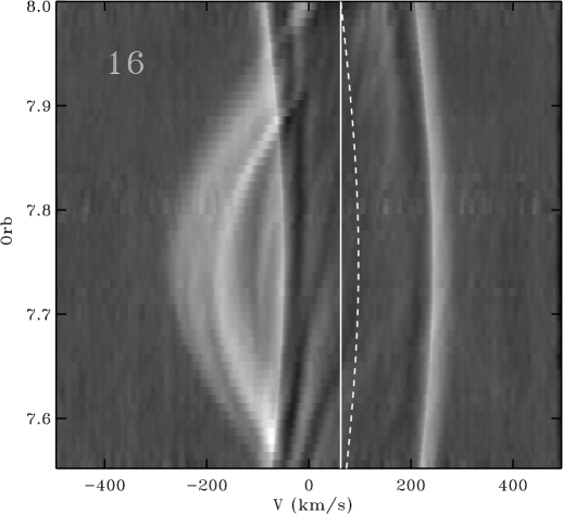
Figure 8: The same as in Figure 5 for the night of 16 July 2018.

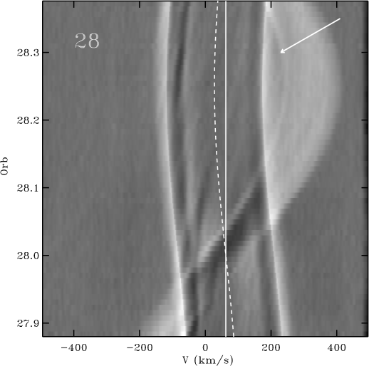
Figure 9: The same as in Figure 5, but after a two-week break in observations, on the night of 28 July 2018. This night included the orbital quadrature when the secondary was receding from the observer. Note the flat profile of the secondary profile at its positive orbital velocities and the faintly defined inner edge of the profile (marked by the white arrow) indicating the velocity field of the secondary component detached from that of the primary component.

Figures 5–9 show the 2D images of the BF time variability on the five nights with more than 40 observations of $\epsilon\,$CrA per night (similar, smaller images exist for the three remaining nights). The images were obtained by interpolation into an equal-step grid of orbital phases with the phase step of 0.008 and then – to improve the visibility of the weak features – by subtraction of the orbital-velocity shifted and scaled rotational-profile fits for the primary component. Figure 10 should be consulted for interpretation of these figures in terms of the sense of rotation and of the orbital phase system. The reader is reminded that a connection of velocities to locations and spatial dimensions is not trivial and requires assumptions.

A comparison of the 2D images of $\epsilon\,$CrA with those of AW UMa in Paper I shows the primary components of both binaries to be very similar to each other, but with some differences: (1) The large-scale disturbances visible as gentle, winding waves on the in the 2D pictures have smaller amplitudes in $\epsilon\,$CrA with the largest intensity modulation of about 4%, while in AW UMa some of them reached 8%; (2) The small-scale ($<\!1\%$), high-frequency, regularly-spaced disturbances which we called “ripples” appear to be absent in $\epsilon\,$CrA; (3) We do not see isolated spots which may have been present on the primary of AW UMa.

We conclude that the primary component of $\epsilon\,$CrA is covered by surface inhomogeneities to a lesser degree than AW UMa. This absence of the wavy ripples, so well visible in AW UMa, is particularly significant as the BF data are of higher quality (the $S/N$ ratio of 120 versus 57 for AW UMa; Section 2) and the overall monitoring time spent on $\epsilon\,$CrA was 3.7 times longer than for AW UMa. However, we should remember that the 3.1 times longer exposure time used for $\epsilon\,$CrA may have led to some smoothing over high frequency disturbances. The pedestal feature of $\epsilon\,$CrA is very similar to that in AW UMa, remaining unexplained.

3.2 The secondary component and the spectroscopic orbit

In contrast to the well understood and basically phase invariable central profile of the rapidly-rotating primary, the secondary component of $\epsilon\,$CrA presents a rather complex picture. Its spectral lines are weak: Expressed as integrals of the respective BF features, the spectral lines are $7.97\pm 0.54$ times weaker than the lines of the primary component, with the large error in this value reflecting the difficulty of separating the two features. While radial velocity profiles of the secondary can be defined in individual BF’s, they are easier to analyze in the 2D images, such as Figures 5–9 where the complexity of the profiles is fully visible thanks to the BF phase intercorrelation. The images show that the secondary component is to some extent connected to its dominating companion, but that the radial-velocity profiles are different than expected for the Lucy model. The profiles suggest a system of gas motions or surface inhomogeneities rather than of an unperturbed, stable photosphere. Spatial localization of these features is generally difficult to establish, but this ambiguity can be sometimes lifted by the eclipses.

A silhouette of the secondary in radial velocities is well defined during the transit (primary, deeper) eclipses ($\phi=0.0$) when the secondary star is projected against its larger companion. We observed transit eclipses on four nights, numbers 12, 13, 16, and 28. The secondary is delineated by two, symmetrically located BF features giving its rotational velocity half-width of $66\pm 2$ km s^-1. We see a considerable difference in the appearance of the two defining “sides” of the secondary component during the transits (see Figures 5, 6 and 9): The negative-velocity side, at $-66$ km s^-1, relative to the secondary mass center, is always more strongly defined by a spike-like feature in the BF’s. A similar, enhanced spectral-line feature was observed in AW UMa, but it is much stronger and better defined in $\epsilon\,$CrA (see the lowest panel of Figure 2). We discuss this feature as a representation of inter-binary gas motions further in Section 3.3.

In contrast to the approaching side, the edge of the rotationally receding side is poorly defined during the transit, but its visibility improves after the primary eclipse when the secondary continues at the positive velocities relative to the projected mass center. These out-of-eclipse phases carry information on the varying velocity distribution over the secondary surface at other aspect angles. Of importance is the admittedly faintly-defined negative-velocity limit of the secondary component when this star is moving away from the observer (the phase range $0<\phi<0.5$; marked by the arrow in Figure 9). It appears that the rotational motion is at least partly confined to the secondary component as if in a local surface motion, without a connection to the velocity field of the primary component. The Lucy model, with its strict solid-body rotation, predicts no separation in velocities of the two components. We saw a very similar inner edge to the secondary-component velocities in AW UMa, but it is much better defined in $\epsilon\,$CrA. This implies that in both binaries the secondary component has its own velocity field, independent of the primary component.

While the secondary component of $\epsilon\,$CrA shows a relatively flat profile at the positive-velocity side of the primary, with numerous but barely-marked and tenuous structures, it is very different when it re-appears after the occultation at $\phi=0.5$. Then, at the negative orbital velocities, it shows a more complicated structure dominated by what appears as a “wisp” in the 2D images (discussed further in the next Subsection 3.3) and as several delicate, phase-dependent weaker features. The individual profiles at negative relative velocities are orbital-phase dependent, with only weak traces of a tendency for a central-depression or meniscus- shaped shape, as was suggested for the less extensively observed for AW UMa. Generally, however, the secondary of $\epsilon\,$CrA does not seem to show a profile similar to that of an accretion disk, as was suggested in Paper I for AW UMa. We note that we probably see the two binaries at orbital inclination angles differing by about ten degrees so that phenomena taking place in the plane of the binary orbit may be visible differently.

Table 4: The spectroscopic orbit of $\epsilon\,$CrA

Parameter	Result	Error	Unit
$P$	0.59145447		day
$HJD(pri)$	2458312.0716	0.0004	day
$K_{1}$	34.718	0.084	km s-1
$K_{2}$	267.13	1.37	km s-1
$V_{0}$	62.541	0.076	km s-1
$q_{\rm sp}=M_{2}/M_{1}$	0.1300	0.0010
$A\sin i$	3.527	0.016	$R_{\odot}$
$(M_{1}+M_{2})\sin^{3}i$	1.685	0.023	$M_{\odot}$
$M_{1}\sin^{3}i$	1.491	0.020	$M_{\odot}$
$M_{2}\sin^{3}i$	0.1938	0.0026	$M_{\odot}$

Note. — The period $P$ was assumed for the epoch of the observations, as described in the text. The time of the deeper (transit) eclipse $HJD(pri)$ is from the primary-component velocity curve. The radial-velocity amplitude of the secondary component was obtained from measurements of the profile centroid locations in 2D images, such as in Figures 5–9, with the value of $V_{0}$ assumed to be the same as for the primary component.

The errors are formal least-squares errors and do not reflect systematic uncertainties in the data – see the text in Section 3.2 for more details.

Table 5: Rotation of the $\epsilon\,$CrA components

	Phase	Observed	$L_{1}$	$L_{2}$	Observer sees
Primary	0.25	147	178	192	primary approaching
	0.5	143	173	184	occultation of the secondary
	0.75	147	178	192	primary receding
Secondary	0.25	89	74	114	secondary receding
	0.0	66	64	75	secondary transits the primary
	0.75	57	74	114	secondary approaching

Note. — The values of the equatorial projected velocity $V\sin i$ are expressed in km s^-1. They were determined by the single-star rotational-profile fits for the primary and as the profile half-widths at the base for the secondary component (see the text). The observed values were determined to approximately $\pm 3$ km s^-1. Predictions of the solid-body rotation values are for the common equipotential surfaces passing through the Lagrangian $L_{1}$ and $L_{2}$ points. The assumed sum of the observed orbital velocities used for the solid-body rotation estimates is $K_{1}+K_{2}=301.9\pm 1.5$ km s^-1. The geometry of the Roche model for $q=0.13$ is from Plavec & Kratochvil (1964).

Table 6: Orbital velocities of the secondary component of $\epsilon\,$CrA

$Time(Orb)$	Vel (km s-1)
0.7638	-211.41
0.7819	-207.11
0.7929	-192.50
0.8214	-178.75
0.8373	-161.56

Note. — The first column gives the time in the $Orb$ units (the time expressed in the binary orbital period; see the text); the second column gives the radial velocity of the secondary component in km s^-1, estimated as a centroid of the secondary profile on the 2D images (see the text).

This table is available in the on-line version only.

The orbital radial velocities of the secondary component were determined from the 2D images (Figures 5–9) for 184 epochs as centroids of the secondary-component profiles. In addition to the orbital motion, we observed variations of the secondary profile in its width and structure, most likely because of the complex gas flows around and over the surface of the secondary component. The secondary profile shows more structure and is narrower after the secondary emerges from behind the primary ($\phi=0.5$) than after the transit over the primary ($\phi=0.0$) when the secondary recedes from the observer.

The individual profiles of the secondary do not appear to be dominated by rotation, as for the primary component, nor do they have shapes expected by the Lucy model. Thus, we cannot directly identify their observed width with $V\sin i$; we can however determine their observed widths from the relatively sharp edges at their BF base. The half-widths of the secondary profiles vary gradually with the orbital phase. The widths can be best established at the phases of the maximum velocity of approach and recession, in addition to the direct radial-velocity imprint at the transit eclipse; the measurements at intermediate phases are more affected by the poor definition of the profile edges and could not be used. The observed half-widths range between 57 km s^-1 at the maximum approach of the secondary ($\phi=0.75$) and 89 km s^-1 at its recession from the observer ($\phi=0.25$); with the half-width at the transit eclipse ($\phi=0.0$) of 66 km s^-1 falling in between. The above numbers carry an uncertainty of about $\pm 3$ km s^-1. The half-widths at the profile base, interpreted as corresponding to $V\sin i$ are summarized in Table 5, together with the half-widths expected for the rigidly-rotating Roche structure; Figure 10 gives a schematic distribution of velocity vectors in the $\epsilon\,$CrA system.

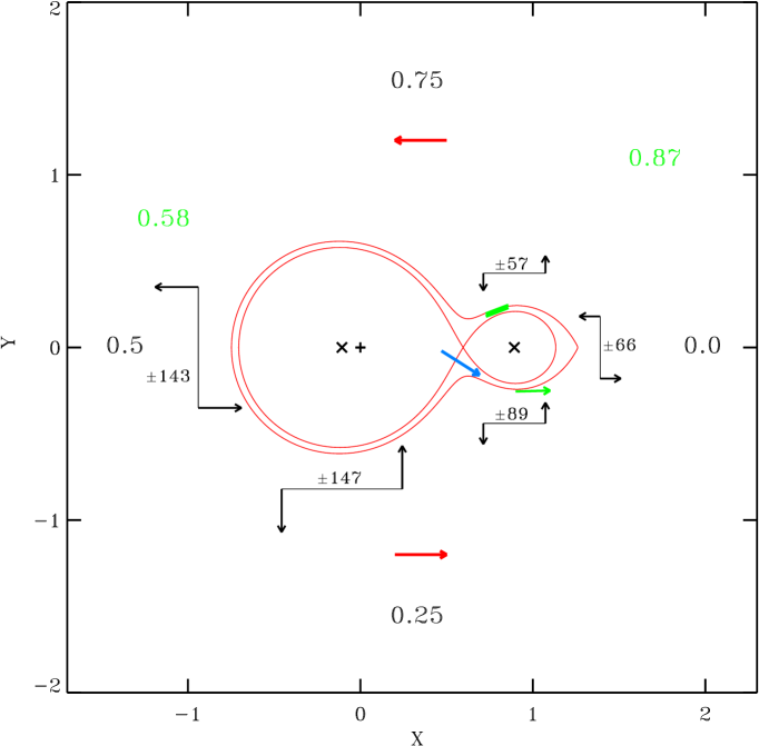
Figure 10: A schematic view of the $\epsilon\,$CrA binary with the observed radial velocities shown as vectors. The unit of geometrical length in the orbital plane is the separation between the mass centers; the velocity vectors are not to scale. The phase directions to the observer are written for four cardinal directions in black. The Roche model equipotentials for $q=0.13$ are shown in red color; the red arrows mark its counter-clockwise rotation of the binary in the figure frame. The individual rotation velocities, such as the $V\sin i$ for the primary and the half-widths at the base for the secondary are written in black as numbers preceded by the $\pm$ sign. The identified sources of the secondary-component profile perturbations are shown in green. The green numbers for the phases correspond to the begin and end of the ”wisp” visibility (see the text). The blue arrow shows the direction of the expected flow originating in the primary component.

The centroid velocities of the secondary component profiles were determined to $\pm 3.5$ km s^-1, as estimated from repeated measurements. They follow the sine curve, as shown in Figure 4. The orbital parameters given in Table 4 assume that the center-of-mass velocity, $V_{0}$, of the secondary is the same as for the primary component. While the uncertainty of $K_{2}$ of $\pm 1.37$ km s^-1 is small, compared with orbital solutions for other W UMa binaries, the single-point error for the secondary, $\pm 14.7$ km s^-1 is large and reflects systematic trends in the deviations within some of the individual orbits reaching $-30$ km s^-1 to $+40$ km s^-1. Since neither the Lucy model nor the simplified sine-curve fits describe such deviations, we treat them as contributors to the random errors. As the result, the orbital parameters presented here should be treated as provisional and subject to re-evaluation once a correct model becomes available. We note that a solution for the secondary with the mean systemic velocity $V_{0}$ treated as a free parameter differed in the mean velocity by $\Delta V_{0}=-0.94\pm 1.77$ km s^-1 from that for the primary component, indicating the overall level of systematic uncertainties in our data processing and velocity measurements.

The quantity which should be least affected by the inadequacy of the adopted model should be the mass ratio, $q=K_{1}/K_{2}$. The light curve synthesis simulations provide information on the mass ratio which is independent of the spectroscopic result; however, it entirely depends on the adopted Lucy-model. The most recent, very accurate photometric value of the mass ratio, $q_{\rm ph}=0.1244\pm 0.0014$ by Wilson & Raichur (2011), is only slightly smaller than our spectroscopic result, $q_{\rm sp}=0.1300\pm 0.0010$; the latter is practically identical with the result by Goecking & Duerbeck (1993), $q_{\rm sp}=0.128\pm 0.014$. Apparently, the systematic difference, $q_{\rm ph}<q_{\rm sp}$, discovered by Niarchos & Duerbeck (1991, Sec.5) is very weakly present in $\epsilon\,$CrA, only at the $4\sigma$ level, and with error estimates which may be systematically too optimistic. Apparently, the similarity of $\epsilon\,$CrA to AW UMa – analyzed in the same way and using the same technique in Paper I – does not extend into the mass-ratio discrepancy. This subject is discussed further in Section 4.1

3.3 Complications in the secondary component profile

The profiles of the secondary component, as shown in Figures 5–9, are fairly complicated yet appear to be surprisingly stable, suggesting a binary-wide velocity field in stationary conditions. However, it is not entirely obvious what is the cause of the details in the profiles. Our Broadening Function information-extraction method is not sensitive to the rarefied gas: It can only detect the presence of a dense, high-temperature gas with similar characteristics to those of the photospheric layers of the primary component. If not projected against a photosphere, the gas must be sufficiently dense to accumulate to the optical depth of at least order of unity along the line of sight to produce an absorption feature detectable by the BF technique. This condition may be fulfilled in localized places close to the secondary component and possibly in the region between the binary components. The radial-velocity measurements give us information about one velocity component of the gas motions only, not about localization of the radiating gas. In addition to the eclipse shadowing effects, a model or plausible assumptions are the only possibilities to visualize the actual patterns of the gas motions.

The BF spike at the negative-velocity of the secondary component during its transit was described in Section 3.2 as defining the approaching side of that star (see the lowest panel of Figure 2). It is one of the most prominent manifestations of the inter-binary matter, but it is visible only in a narrow range of phases around $\phi=0.0$, becoming the strongest at the exact alignment of the stars. Its phase dependence is difficult to measure because the spike is small in the absolute sense with the integrated intensity at its maximum of less than one percent of that of the primary-component integrated profile. If strengthening of the spectral lines was coincident with a continuum increase, such a faint feature would be detectable in broad-band photometry, possibly combining with other small variations during the eclipse branch. In the case of the current program, it was possible to detect it spectroscopically mostly thanks to the linear properties of the BF technique and after subtraction of the dominant primary-component profile. Its width at the base is $25\pm 2$ km s^-1, as estimated from repeated transit events. We think that the spike is produced by the outer layers of a stream of matter flowing away from the primary component and sliding along the surface of the secondary, directly towards the observer. The outer layers of the flow attain a sufficient optical depth when visible along and into their length; they must be relatively slim and long to produce a strong dependence on the angle.

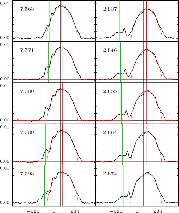
Figure 11: The Broadening Functions illustrate the secondary-profile complication visible as a radial-velocity feature called a “wisp” in the text. The wisp is interpreted as a radial-velocity representation of a stationary area of the enhanced absorption spectrum. The left column shows a sequence for the orbital phase around $\phi\simeq 0.58$ when the wisp appears after the secondary occultation while the right column shows the orbital phases close to $\phi\simeq 0.86$ when the projection of the secondary component starts approaching its transit over the primary component. The vertical red and green straight lines give the orbital velocities of the mass centers of the primary and secondary components determined by the sine-function fits, while the black line gives the velocity of the binary center. The rotational profile of the primary for $V\sin i=147$ km s^-1 is shown by a thin red line. The $Orb$ number is given in the left upper corner of each panel; its fractional part is the orbital phase.

The radial-velocity profile of the secondary component appears to be more complicated within the orbital phases when the secondary approaches the observer (the phase interval $0.5<\phi<1.0$). The most prominent feature visible in the radial velocity images in Figures 5–9 is called here a “wisp” (see also the third panel of Figure 2 and Figure 11). The wisp emerges from behind the primary component around the orbital phase $\phi\simeq 0.58$ and remains visible to $\phi\simeq 0.87$. The phases of the wisp appearance and disappearance are the only positional indications on the location where the wisp is formed, but these limiting phases are difficult to determine; they are coincident with the intervals when the radial-velocity measurements of the primary component required rejection of several discrepant measurements from the final velocity curve (Figure 4).

The wisp has very different properties from the brief BF spike at the binary-component alignment producing the transit eclipse: It is not rapidly changing its intensity with the orbital phase, instead, it shows a systematic drift in radial velocities within its visibility phase range, $0.58<\phi<0.87$ (the best visible in Figure 6; see also Figure 11). It stays confined to the middle of the secondary-component profile suggesting a feature possibly anchored on the stellar disk and apparently confined to one hemisphere since it does not reappear on the positive-velocity side of the system when the secondary component recedes from the observer ($\phi>0.0$). The wisp tends to be wider soon after its emergence from behind the primary component, with the full width at the base of about 35–40 km s^-1, then it narrows down to 15–20 km s^-1 before its disappearance. Its migration in the radial velocities relative to the center of mass of the secondary component can be approximated by a linear dependence on the orbital phase, ${\rm Drift}=29.24(\pm 0.64)+217.50(\pm 6.53)\times(\phi-0.75)$ km s^-1 km s^-1 (Figure 12), where the single-measurement error of the relation, 3.3 km s^-1, is mostly due to measurements uncertainties.

Figure 12: Radial velocities of the “wisp” visible in the 2D images in Figures 5–9 within the orbital-phase range when the secondary component approaches the observer. The Drift velocity is expressed relative to the orbital velocity of the secondary component.

Assuming the projected rotational velocity of the secondary component of $-66$ km s^-1 and the orbit-synchronous rotation, the constant intensity and the apparent radial-velocity drift of the wisp can be explained by a spatially-stationary patch located on this component and visible for half of the orbital revolution. This patch of an increased strength of the spectral lines would be then located on the positive Y-axis side in Figure 10, at about $60-65$ degrees away from the line joining the stars. This location would explain why the patch is invisible within the orbital phase range $0<\phi<0.5$, as well as the early appearance after the mid-occultation at $\phi=0.58$ and an even-earlier disappearance before the mid-transit at $\phi=0.87$. These numbers assume a moderately low orbital inclination angle of $i\simeq 70$ degrees producing a grazing totality eclipse. The wisp, as a positive BF feature with the strength of about $1.5-2$% of the primary component integrated BF intensity, is produced by a localized enhancement of the absorption line spectrum. Although it is so weak, its strength is not negligible relative to the secondary-component where it contributes up to 20% of the integrated BF intensity.

The input spectra were individually normalized (to the unit level at the observed continuum) so that without simultaneous photometric observations we can only state that the spectral lines become stronger during the visibility of the wisp. But the mechanism is not known as the lack of an independent information on the continuum precludes a proper interpretation of the wisp. We see two possible explanation of the enhanced spectrum producing the wisp:

1. The patch of the stronger lines is produced by a localized piling up of the dense gas. Normally, added material on top of the atmosphere would simply shift the location of the surface corresponding to the optical-depth of one. But, since we do not know the exact geometry of the gas circulation in the $\epsilon\,$CrA system, this may be a viable solution. The broad-band photometric effect of such a gas concentration is expected to be very small at a level of $\leq 0.1$% since the wisp corresponds to a $\leq 2$% modification of the spectrum whose integrated equivalent width of all spectral lines in our spectral window is about 5.5% relative to the continuum level.

2. A spot of a depressed effective temperature. The locally lower temperature would lead to a decrease of the star brightness and to a richer and stronger absorption-line spectrum. Our spectra were normalized so that information on the stellar brightness was lost. This matter could not be resolved without broad-band data, but we have indirect indications (see the next Section 3.4 and Figure 13) that the light-curve maximum after the secondary eclipse ($\phi\simeq 0.75$) was by about 2% lower than the first maximum. This would suggest that the wisp-causing dark spot may have indeed influenced the continuum level. Such a spot would be most likely very different from magnetic star spots because the effective temperature drop must be rather moderate. Usually magnetic spots are dark and it is hard to detect their spectral contribution, whereas here the line-spectrum enhancement would over-compensate for the brightness decrease.

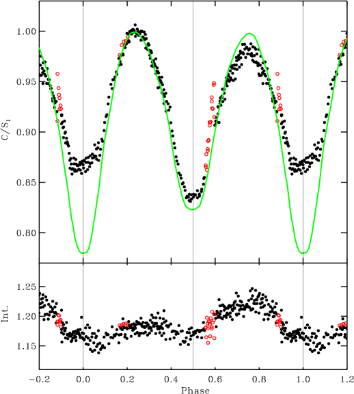
Figure 13: The “light curve” of $\epsilon\,$CrA restored from the BF spectral data (upper panel) and the phase variations of the integrated equivalent width (IEW) of the spectral lines; see the text for details. The red, open circles mark the data not used for the radial-velocity orbit determination. The green line shows the visual-band light curve obtained by Knipe (1967) after conversion to flux units.

3.4 The spectroscopic “light curve”

We demonstrated for the case of AW UMa (Paper I) that, with some assumptions, the spectroscopic results can give a direct link to the photometric phase variability of this binary. We utilized (1) the BF normalization of the integrated equivalent width (IEW) of all spectral lines in the spectral window to the IEW of the model spectrum, and – building upon the observed approximate constancy of the effective temperature with the orbital phase, (2) we made a strong assumption that the spectral lines of the primary component remain constant with the orbital phase. The results for $\epsilon\,$CrA are shown in Figure 13, while additional explanations of the two assumptions are as follows:

1. The BF’s for AW UMa and $\epsilon\,$CrA were determined using the same model atmosphere, F2V for the solar abundance. The IEW in AW UMa showed only a very small IEW phase variation of about 2% around the value of 1.10 (Figure 2, Paper I). This agreed with the approximate effective-temperature constancy and could be interpreted as a slightly later spectral type of AW UMa than of the template. In $\epsilon\,$CrA, the IEW is larger, with the mean value of 1.18 (Figure 13), in agreement with suggestions of an even later spectral type of the binary. The IEW shows about 5% departures from the mean value reaching 1.23 at the orbital phases around $\phi\simeq 0.75$. We note that these are the phases when the secondary component approaches the observer and when the wisp-producing feature (Section 3.3) could influence the continuum spectrum; apparently, the feature produces stronger absorption lines as if the local effective temperature was lower. The IEW for $\epsilon\,$CrA is not as invariable with phase as that for AW UMa; the difference between the binaries may possibly relate to their different orbital inclination angles and the different visibility of their orbital planes where – according to the model of Stȩpień (Section 4.2) – the energy is transported between the binary components.

2. The assumption (2) states that the primary component does not change with the orbital phase and remains a rapidly rotating star describable by a rotational profile; it is oblivious to the existence of the secondary component. In other words: Whatever happens in the system in terms of the line producing photospheric area is due to the secondary and the matter around it. The assumption is made simply for convenience; its correctness is verifiable by the result.

The “spectroscopic light curve” is calculated using the maximum value ($S_{1}$) of the primary component rotational-profile to form a phase dependence of its inverse $C/S_{1}$ (see the discussion in Paper I, Sec. 3). It turns out that such dependence is a very reasonable approximation to the photometric light curve, as shown in the upper panel of Figure 13, confirming our assumptions. In Paper I, we used for $C$ the normalized integral of the rotational profile, but here we simply use an arbitrary constant adjusted to produce a light curve normalized to unity at the maximum light. Such a light curve is correctly phased and can be compared with the calibrated light curves of Knipe (1967) (shown in Figure 13), Tapia (1969) and Hernández (1972). Only the primary (transit) eclipse comes out too shallow, but this is expected since the assumption of no apparent change to the primary component profile breaks down during these phases.

In very simple terms, the “spectroscopic light curve” derived in the above way expresses the amount of the spectral-line producing surface projected onto the sky. Figure 13 tells us that this amount is very close to what can be calculated using the Lucy model. Thus, such a spectroscopically-derived light curve does carry the same information about the binary – but admittedly in a more convoluted way – as a standard photometric light curve.

The successful application of our approach may turn out to be restricted to the low mass-ratio systems such as our two targets, AW UMa and $\epsilon\,$CrA, where the primary components strongly dominate in the energy balance. However, thanks to the steep mass-luminosity relation in the lower Main Sequence, the domination of the primary component may extend into moderate mass ratios. The binary parameter range for the above approach remains to be determined.

4 Conclusions

4.1 $\epsilon\,$CrA and AW UMa

The new, spectral time-monitoring observations of $\epsilon\,$CrA show the binary as a twin to AW UMa analyzed in Paper I. The observations were more extensive (3.1 times more total exposure time) and more accurate (the observational $S/N$ improved about twice) so that the results carry more weight in a discussion of both binaries. $\epsilon\,$CrA appears to be slightly more massive, as expected for a longer orbital period, but the spectral types are practically identical, although $\epsilon\,$CrA may have more evolved cores judging by its larger luminosity and the slightly lower effective temperature. The two binaries are very similar in having small mass ratios ($q_{\rm sp}=0.10$ and 0.13). Most importantly, both show an identical disagreement with the assumptions of the Lucy model by having an apparently stationary velocity field in the rotating frame of the binary. The gas flows are best visible within the secondary-component profile and in the volume between the components. We did not see any obvious changes in the flow velocity patterns over 27 orbital periods so $\epsilon\,$CrA may have more stable internal velocities than AW UMa; the latter, however, was not observed equally extensively as $\epsilon\,$CrA. In $\epsilon\,$CrA, a “wisp” (Section 3.3) in the 2D time-sequence images of the surface velocity motions, associated with the secondary component was seen to be stable over the duration of the observations. Similar, but less well-defined velocity features were seen in AW UMa. Such features are most probably produced by gas streams seen along their longer dimensions through accumulated optical depth or may come from isolated areas of enhanced spectral-line strength of currently unexplained properties.

The general stability of both binaries is confirmed by the moderate systematic period variations, with $dP/dt$ at a level of a few $\times 10^{-7}$ day/year. The period changes in these two binaries are of opposite sign, hence they are most likely unrelated to their secular evolution. They may be explainable by a small imbalance in the net mass transfer between the binary components or by external perturbations; we recall that W UMa binaries practically always exist in triple systems, see Tokovinin et al. (2006) and Rucinski et al. (2007). Since large amounts of matter carrying radiation energy appear to circulate between the components (see the next Subsection 4.2), the flows must be well balanced in terms of the net amount of the matter transferred between the stars.

The primary in both binaries is a rapidly-rotating early F-type star with the projected equatorial rotational velocity $V\sin i$ at about 80% of the rate synchronous with the orbital motion (cf. Section 3.1). The BF profile appears symmetric and well represented by the standard rotational profile. The slower-than-expected rotation suggested for the higher latitudes of the primary may partially result from the anti-cyclonic gas motion (in the counter-rotation direction) seen in the mass-losing, hydrodynamic models of Oka et al. (2002). Gas velocities in such a high-pressure cell are expected to link the high stellar latitudes of the primary to the outflow from the Lagrangian $L_{1}$ point. Only a modest reduction of the observed rotational velocity is expected however, perhaps by a value of the order of sonic or subsonic photospheric velocity which for the spectral types of both stars is $\simeq 7$ km s^-1. The pedestal at the base of the primary rotational profile with the additional broadening by 25–35 km s^-1 would bring the observed $V\sin i$ into an approximate agreement with the synchronous rate with the orbit. The pedestal contributes moderately to the total depth of the spectral lines, typically at a level 0.06 to 0.10 of the integrated rotational profile of the primary. The pedestal likely reflects the presence of the matter in the orbital plane, returning to the primary after its orbit around the secondary component.

The secondary components of W UMa-type binaries are important for our understanding of the unresolved secret of how these binaries function as stable structures. The secondaries of both, $\epsilon\,$CrA (Section 3.2) and AW UMa (Paper I), look similar in that they show orbital-phase changes which are repeatable and stable in time, and appear to be related to the phase-dependent visibility of an otherwise stationary velocity field. We identified two features in the somewhat complex radial velocity picture: (1) A stream directed toward the observer over the secondary surface, accumulating to sufficient optical line depth within a narrow cone of visibility; (2) A region where the absorption line spectrum is for some reason stronger than in the surrounding; it can be a region of a local, geometrically complex piling up of the gas possibly through collision of a direct and circum-secondary flows from the primary, or an area of a slightly lower effective temperature with enhanced absorption line spectrum. These features may be the sought-after surface imprints of a deeper energy transport from the primary to the secondary component. In spite of the complex radial-velocity picture, the amount of the visible, line-producing photosphere of the secondary and of the matter between the stars approximately agrees with that predicted by the Roche-model based model of Lucy (1968b).

4.2 A new model for W UMa binaries?

Our observational results for AW UMa and $\epsilon\,$CrA relate to two small mass-ratio W UMa-type systems. Despite their small mass ratios, both binaries have been always considered genuine members of and representatives for the whole class of these objects. We assume that our results indeed apply to the whole class of the W UMa-type binaries.

The available radial-velocity data for AW UMa and $\epsilon\,$CrA show that the main assumption of the Lucy (1968a, b) model, the solid-body rotation of the components as a prerequisite for the definition of the Roche-model equipotentials, is not confirmed. A complex system of velocities in the rotating system of coordinates is particularly well visible within the phase-dependent radial-velocity profiles of the secondary component. The velocities are moderate, of the order of or less than the rotational velocity of the secondary component while their observed ranges are of the order of the local sound speed. But their spatial pattern is of great importance as we see circulation fully confined to the secondary component, similar to that expected on a non-contact binary component. The impact of such well organized velocity systems on the assumed W UMa-binary model and on interpretation of light-curve observations is currently unknown and should be investigated.

The solid-body assumption at the time of the Lucy model creation was simply the easiest to make, although no mechanism had been offered why the components would rotate in such a way. This assumption made the Lucy model particularly easy to use as a light-curve modeling tool so that many light-curve solutions have been made utilizing the model’s simplicity. Most of these solutions produced photometric mass ratio, $q_{\rm ph}$, determinations utilizing the one-to-one mapping between the mass ratio and the relative dimensions of the components, first discussed by Mochnacki & Doughty (1972). While this relationship has been particularly useful for light-curve solutions, it appears that it may require a correction or modification. This had been signalled by Goecking & Duerbeck (1993), was strongly confirmed for AW UMa and is now indicated for $\epsilon\,$CrA. While the discrepancy between the spectroscopically determined $q_{\rm sp}$ and photometrically $q_{\rm ph}$ for $\epsilon\,$CrA is indicated at the level of $4\times\sigma$ (with possibly over-optimistic error estimates), for AW UMa the relative discrepancy $(q_{\rm sp}-q_{\rm ph})/q_{\rm sp}$ reached the unbelievable relative value of $\geq 10$%! This suggests that either the spectroscopic or photometric determinations of $q$ may be biased. We point out that unrecognized, but omnipresent companions tend to push photometric solutions towards smaller mass ratios and/or smaller orbital inclinations by a photometric-scale change; no equally simple biasing mechanism exists for spectroscopic mass-ratio determinations executed at an adequate resolution. Whatever the reason, the continuing routine use of the Roche-lobe based photometric model to determine the values of $q_{\rm ph}$ may give systematically wrong individual results, biasing statistics of the mass ratio, masses and orbital inclination angles.

The Lucy (1968a, b) model, when it was developed more than a half-century ago, offered the first physically acceptable description of W UMa-type binaries. It generated an extensive interest, but also considerable controversy after its implied properties were studied in more detail. The main difficulties were related to the internal structure and effective-temperature equalization processes. Further research led to the consideration of the thermal cycles consisting of semi-detached and contact configurations (Lucy, 1976; Flannery, 1976), but the problems did not disappear, but related to the structure during a part of the thermal cycle, after re-establishment of the contact. The discussion culminated in detailed studies of the energy transport in contact by Webbink (1976, 1977) and a heated discussion of the concept of a “contact discontinuity” (Shu et al., 1976; Hazlehurst & Refsdal, 1978; Papaloizou & Pringle, 1979; Shu et al., 1979). The “discontinuity” concept was important as it envisaged the secondary component fully enshrouded in the matter of the primary component. This assumption solved the equality of the effective temperatures while the rest of the observables, particularly the solid-body-rotating equipotential structure, remained as in the original Lucy model. The end to further discussion and similar first-principle considerations came from the realization that – with only photometric data – there exist no observational verification methods for this complex problem. The model concept of Stȩpień (2009) returned to the idea of the gas of the primary-component surrounding the secondary, but now not as a static equipotential structure, but rather as a stationary flow of the optically-thick matter confined to the equatorial regions and eventually returning to the primary. In its motion, the flow is controlled by the gravitational pull to the orbital plane and the dispersing tendency of the Coriolis force in the plane. The Stȩpień study specifically addressed the energy transport requirements and did not offer any predictions on the observational consequences of the flow, making his ideas less directly applicable at the present stage than the Lucy model.

Our detection of the organized gas flows in AW UMa and $\epsilon\,$CrA supports the energy-transport model of Stȩpień (2009) and the pioneering hydrodynamic calculations of Oka et al. (2002). The essential component of a new vision is a stationary flow that dominates the thermal equilibrium of the binary and which starts and ends on the primary component. The flow submerges the equatorial regions of the secondary in optically thick gas. It leaves the primary at high latitudes to slide down to the low latitudes of the $L_{1}$-point region where it starts its orbit around the secondary component, first curving to one side of the binary (the negative Y-axis side in Figure 10), and then returning to the primary at its low latitudes. When all the matter returns to the primary and there is no net mass-transfer between the components, then no orbital period changes are expected to be observable. The stream at its return may lead to formation of the perturbed region identified between the stars in $\epsilon\,$CrA; it may also excite the standing atmospheric waves visible as the ripples in AW UMa. We see only the outermost layers of the moving matter, although the process may involve large amounts of matter carrying substantial energy. Generally, only moderate observable effects are expected, such as those we detected in AW UMa and $\epsilon\,$CrA, but some details are not easily explainable, e.g. the phase-dependent velocity extent of the secondary component.

Two directions can be followed for further research to develop modifications of the current W UMa-binary model: The theoretical one specifically addressing the detailed properties of the Stȩpień energy-transfer model, perhaps following the directions established by the pioneering hydrodynamical models of Oka et al. (2002) and the observational one based on high-resolution time-sequence spectroscopy. Both may present considerable difficulties. The former would require extensive use of super-computers in a simulation incorporating complex physical phenomena, while the observations would be difficult to arrange as they require relatively large amounts of time on moderate- or large-size telescopes equipped with high-efficiency, high-resolution spectrographs. As always, the observations would provide the necessary guidance, but are harder to generalize than theoretical models. The result of the effort is expected to lead to a paradigm shift from an elegant picture of a static, solid-body, Roche-model structure with the inexplicable equality of temperature over its surface, to a more complex vision of a gaseous binary approximately agreeing with the Roche model, with the primary component engulfing the secondary component in its equatorial regions by an optically thick, stationary flow carrying the temperature-equalizing energy.

References

- Eaton (2016) Eaton, J. A. 2016, MNRAS, 457, 836
- Flannery (1976) Flannery, B. P. 1976, ApJ, 205, 217
- Gaia Collaboration (2016) Gaia Collaboration, A&A, 595, 1
- Gaia Collaboration (2018) Gaia Collaboration DR2, A&A, 616, 1
- Goecking & Duerbeck (1993) Goecking, K.D., & Duerbeck, H.W. 1993, A&A, 278, 463
- Grey et al. (2006) Gray, R. O., Corbally, C. J., Garrison, R. F., McFadden, M. T., et al. 2006, AJ, 132, 161
- Hazlehurst & Refsdal (1978) Hazlehurst, J. & Refsdal, S. 1978, ApJ, 62, L9
- Hernández (1972) Hernández, C. A. 1972, AJ, 77, 152
- Knipe (1967) Knipe, G. C. F. 1967, Rep. Obs. Johann. Circ. 126, 142
- Lucy (1968a) Lucy, L. B. 1968a, ApJ, 151, 1123
- Lucy (1968b) Lucy, L. B. 1968b, ApJ, 153, 877
- Lucy (1976) Lucy, L. B. 1976, ApJ, 205, 208
- Mochnacki & Doughty (1972) Mochnacki S.W., & Doughty N.A. 1972, MNRAS, 156, 51
- Niarchos & Duerbeck (1991) Niarchos, P. G. & Duerbeck, H. W. 1991, A&A, 247, 399
- Oka et al. (2002) Oka, K., Nagae, T., Matsuda, T., Fujiwara, H., & Boffin, H. M. J. 2002, A&A, 394, 115
- Papaloizou & Pringle (1979) Papaloizou, J. & Pringle, J. E. 1979, MNRAS, 189, 5P
- Plavec & Kratochvil (1964) Plavec, M., & Kratochvil, P. 1964, Bull. Astr. Inst. Czechoslovakia, 15, 165
- Pribulla & Rucinski (2008) Pribulla, T., & Rucinski, S. M. 2008, MNRAS, 386, 377
- Rucinski (2002) Rucinski, S. M. 2002, AJ, 124, 1746
- Rucinski (2010) Rucinski, S. M. 2010, in Binaries – Key to Comprehension of the Universe, eds. A. Prša, M. Zejda, ASP Conf. Ser. 435, 195
- Rucinski (2012) Rucinski, S. M. 2012, in From Interacting Binaries to Exoplanets: Essential Modeling Tools, eds. M. Richards, & I. Hubeny IAU Symp., 285, 365
- Rucinski (2013) Rucinski, S. M. 2013, AJ, 146, 70
- Rucinski (2015) Rucinski S. M. 2015, AJ, 149, 49 (Paper I)
- Rucinski et al. (2007) Rucinski S. M., Pribulla, T., van Kerkwijk, A. H. 2007, AJ, 134, 2353
- Rucinski et al. (2013) Rucinski S. M., Matthews, J. M., Cameron, C., Guenther, D. B., et al. 2013, Inf. Bull. Var. Stars, 6079
- Shu et al. (1976) Shu, F. H., Lubow, S. H., & Anderson, L. 1976, ApJ, 209, 536
- Shu et al. (1979) Shu, F. H., Lubow, S. H., & Anderson, L. 1979, ApJ, 229, 223
- Stȩpień (2009) Stȩpień, K. 2009, MNRAS, 397, 857
- Tapia (1969) Tapia, S. 1969, AJ, 74, 533
- Tokovinin et al. (2006) Tokovinin, A., Thomas, S., Sterzik, M., & Udry, S. 2006, A&A, 450, 681
- Tokovinin et al. (2013) Tokovinin, A., Fischer, D. A., Bonati, M., Giguere, M. J., et al. 2013, PASP, 125, 1336
- Tapia & Whelan (1975) Tapia, S. & Whelan, J., 1975, ApJ, 200, 98
- Twigg (1979) Twigg, L. W. 1979, MNRAS, 189, 907
- Webbink (1976) Webbink, R. F. 1976, ApJS, 32, 583
- Webbink (1977) Webbink, R. F. 1977, ApJ, 215, 851
- Wilson & Raichur (2011) Wilson, R. E., & Raichur, H. 2011, MNRAS, 415, 596