New method for fitting the low-energy constants in chiral perturbation theory

Abstract

A new set of the next-to-leading order (NLO) and the next-to-next-to-leading order (NNLO) low-energy constants $L_{i}^{r}$ and $C_{i}^{r}$ in chiral perturbation theory is obtained. These values are computed using the new experimental data with a new calculation method. This method combines the traditional global fit and Monte Carlo method together. The higher order contributions are estimated with this method. The theoretical values of the observables provide good convergence at each chiral dimension, except for the NNLO values of the $\pi K$ scattering lengths $a_{0}^{3/2}$ and $a_{0}^{1/2}$. The fitted values for $L_{i}^{r}$ at NLO are close to their results with the new method at NNLO; i.e., these $L_{i}^{r}$ are nearly order-independent in this method. The estimated ranges for $C_{i}^{r}$ are consistent with those in the literature, and their possible upper or/and lower boundaries are given. The values of some linear combinations of $C_{i}^{r}$ are also given, and they are more reliable. If one knows a more exact value $C_{i}^{r}$, another $C_{i}^{r}$ can be obtained by these values.

I Introduction

Chiral perturbation theory (ChPT) is an important tool to study the low-energy pseudoscalar mesonic interactions. The main idea of ChPT comes from the fact that QCD possesses an $SU(3)_{L}\times SU(3)_{R}$ flavor symmetry in the chiral limit in which the light quark are considered massless. This symmetry is spontaneously broken into the subgroup $SU(3)_{V}$ and eight massless pseudoscalar Goldstone bosons arise. These pseudoscalar Goldstone bosons are considered to be the lightest eight pseudoscalar mesons ($\pi$, $K$ and $\eta$). The small masses of these pseudoscalar mesons come from the small light-quark masses. On the other hand, the fundamental interaction between the pseudoscalar mesons in ChPT can be considered as an effective interaction in the low energy, i.e. ChPT is only an effective theory. The only restriction is symmetry, such as chiral symmetry, parity symmetry, charge conjugation symmetry, and so on. There exist an infinite number of terms satisfying these symmetries, and an infinite number of unknown parameters called low-energy constants (LECs) that correspond to these terms. The details of the strong interaction are hidden in these LECs. The Weinberg power-counting scheme organizes the most important terms to be considered first, the second important ones to be calculated secondly, and so on Weinberg (1979). Generally, physical quantities in ChPT are calculated order by order (chiral dimension). One order provides about a $p/\Lambda_{\chi}$ factor, where $p$ is the typical scale of the momentum and $\Lambda_{\chi}\sim 1$ GeV is the scale related to chiral symmetry breaking. For the three-flavor ChPT, there exist 2, 10+2, 90+4, and 1233+21 LECs in the $\mathcal{O}(p^{2})$, $\mathcal{O}(p^{4})$, $\mathcal{O}(p^{6})$, and $\mathcal{O}(p^{8})$ order, respectively Gasser and Leutwyler (1985, 1984); Bijnens et al. (1999, 2019). The numbers after the plus signs are related to the contact terms. It shows that the numbers increase rapidly with the growth of the chiral dimension. Nevertheless, ChPT can not determine these LECs by itself. Without LECs, most physical quantities would not be calculated numerically and ChPT would lose most of its predictions. Hence, numerical values of LECs play an important role in ChPT. There are a lot of methods to obtain LECs, such as global fit Bijnens et al. (1994); Amorós et al. (2000a); Bijnens and Jemos (2012); Bijnens and Ecker (2014), lattice QCD Dowdall et al. (2013); Bazavov et al. (2010a, 2009, b); Bernard and Passemar (2010), chiral quark model Jiang et al. (2010, 2015), resonance chiral theory Amorós et al. (2000b); Knecht and Nyffeler (2001), sum rules Golterman et al. (2014), holographic QCD Colangelo et al. (2012), dispersion relations Guo et al. (2007, 2008); Guo and Sanz-Cillero (2009), and so on. Each method has its advantage and application domain. However, at present, most of them only obtain a part of LECs at/to a given order and the higher-order contributions are neglected. Most numerical results satisfy the power-counting scheme, but there also exist some exceptions (see the discussion below). However, the calculation at/to a given order sometimes may not give a very good prediction. It leads to numerical values of some LECs that may have large errors. This is one possibility why some LECs have large errors in some references. One motivation for this paper is to obtain some LECs with the higher-order contributions in order to narrow the errors of some NLO LECs.

In this paper, some three-flavor LECs will be obtained with a new method, which is similar to the traditional global fit method but with some improvements. The traditional global fit method seems simpler than the pure calculation by the background theory. This method is also much closer to the experiment, because it fits the experimental data directly. The theoretical values and errors can be obtained simultaneously without the background theory or any other physical model. Usually, $\chi^{2}$ in the fit is as small as possible, and the corresponding LECs are the result. However, the global fit method needs sufficient theoretical calculations in ChPT, some of them which may be in the high order with tedious loop-diagram calculations. Its precision is limited by the number and the accuracy of experimental data. So far, a lot of research arises and some LECs have been fitted. $L_{1}^{r}$, $L_{2}^{r}$ and $L_{3}^{r}$ are obtained by fitting $K_{\ell 4}$ form factors and $\pi\pi$ scattering lengths Bijnens et al. (1994). $L_{i}^{r}(i=1,2,3,5,7,8)$ are obtained by fitting the quark-mass ratio $m_{s}/\hat{m}$, the decay constant ratio $F_{K}/F_{\pi}$ and $K_{\ell 4}$ form factors Amorós et al. (2000a). About ten years later, Ref. Bijnens and Jemos (2012) added $\pi\pi$ scattering lengths ($a_{0}^{0}$ and $a_{0}^{2}$), $\pi K$ scattering lengths ($a_{0}^{1/2}$ and $a_{0}^{1/3}$) and the threshold parameters of the scalar form factor ($\langle r^{2}\rangle_{S}^{\pi}$ and $c_{S}^{\pi}$) in the fit. Recently, Ref. Bijnens and Ecker (2014) added two-flavor LECs in the fit. The last two references not only obtain the next-to-leading order [NLO, $\mathcal{O}(p^{4})$] LECs $L_{i}^{r}$ but also estimate a part of LECs $C_{i}^{r}$ in the next-to-next-to-leading order [NNLO, $\mathcal{O}(p^{6})$]. Nevertheless, their results only make use of the theoretical expansion to a finite order (NNLO). The higher-order contributions are ignored. There also exist some other problems in Ref. Bijnens and Ecker (2014):

1. Some NLO fitted values of $L_{i}^{r}$ are quite different from those obtained at NNLO. For example, $L_{1}^{r}=0.53(06)\times 10^{-3}$ at a NNLO fit, which is about half of its NLO fitted value $L_{1}^{r}=1.0(1)\times 10^{-3}$. Nevertheless, $L_{1}^{r}$ is a constant. Its true value is order independent. Its fitted value should not depend on the order as far as possible.

2. The higher-order effects are not taken into account. If the higher-order corrections are considered, some physical quantities may change largely, such as $a_{0}^{1/2}$ and $a_{0}^{3/2}$. Reference Bijnens and Ecker (2014) tells us that the numerical values of $a_{0}^{1/2}$ and $a_{0}^{3/2}$ at NNLO are larger than the NLO results. Hence, the higher-order effects should have a big impact on the low-order LECs. In addition, one can determine whether a set of LECs have reliable values, if the higher-order effects are known. If the possible higher-order effects are smaller than the low-order ones, the set of LECs should be considered more reliable. Hence, the higher-order effects should play an important role in the fit.

3. The fitted $\chi^{2}/\mathrm{d.o.f.}$ is approximately equal to $1.0/10$ at NNLO fit. There seems to be an overfitting problem. A larger $\chi^{2}$ could give a wider range of $C_{i}^{r}$. Some $C_{i}^{r}$ in this wider range may solve the two problems discussed above.

4. The $\pi K$ scattering lengths $a_{0}^{1/2}$ and $a_{0}^{3/2}$ have a poor convergence. Compared with the NLO results, their NNLO values are too large.

5. Some original data about $C_{i}^{r}$ Bijnens (2019) are very close to the final results Bijnens and Ecker (2014). The differences are less than $10^{-12}$. We guess these LECs might be dependent on the boundaries.

In this paper, we attempt to solve the first three problems and try to find out why the other two problems arise. With some reasonable hypotheses, a new method for fitting LECs is introduced and a set of $L_{i}^{r}$ and $C_{i}^{r}$ are obtained. Because the number of constraint conditions is not large enough, only the ranges of $C_{i}^{r}$ are obtained, but the values of $L_{i}^{r}$ are more precise.

This paper is organized as follows: In Sec. II, some hypothesises are introduced and the following calculations are based on these hypothesises. In Sec. III, all the experimental data involved are given. Section IV introduces a modified global fit method with the higher-order estimation. In Sec. V, some rough values of $L_{i}^{r}$ are given and the convergences of some observables are also presented. In Sec. VI, a new method is introduced, which can compute more reasonable values of $L_{i}^{r}$ and estimate the values of $C_{i}^{r}$. Section VII gives the results of $L_{i}^{r}$ and $C_{i}^{r}$ with this new method. A short summary is given in Sec. VIII

II The low-energy constants and their hypotheses

In ChPT, without the contact terms, for the three-flavor case, there are 10 LECs $L_{i}$ at NLO and 90 LECs $C_{i}$ at NNLO; for the two-flavor case, 7 LECs $l_{i}$ exist at NLO and 52 LECs $c_{i}$ exist at NNLO. Their renormalized values $L_{i}^{r}$, $C_{i}^{r}$, $l_{i}^{r}$ and $c_{i}^{r}$ are defined in Refs. Gasser and Leutwyler (1984, 1985); Scherer and Schindler (2012); Bijnens (2013); Bijnens and Ecker (2014); Bijnens et al. (2000). Some scale independent $\bar{l}_{i}$ Gasser and Leutwyler (1984) are used frequently. This paper will determine the values of 8 $L_{i}^{r}\;(i=1,\ldots,8)$ and 38 $C_{i}^{r}$ (the values of $i$ can be found in Table 5) at the renormalization scale $\mu=0.77$GeV. Four $\bar{l}_{i}\;(i=1,2,3,4)$ will be used in the estimation as observables, and none of the $c_{i}$ will be used. The following notations are the same as those in Ref. Bijnens and Ecker (2014).

Due to the experimental condition and the theoretical calculation, the experimental data and the relevant NNLO analytical results are lacking. Until now, only 17 observables have been used in the NNLO global fit Bijnens and Ecker (2014). Theoretically, it is impossible to obtain all LECs very accurately with only these 17 observables. Hence, we have different requirements for these NLO and NNLO LECs. For $L_{i}^{r}$, their values need to be as precise as possible, because their number (8) is much less than 17. On the other hand, although 17 is less than 38, it does not seem too small to estimate $C_{i}^{r}$. With the help of some reasonable hypotheses, the intervals of $C_{i}^{r}$ can be limited to some reliable ranges at least. To achieve these goals, the following hypotheses are introduced to limit the feasible ranges of the LECs:

1. Chiral expansion for most observables is assumed to have good convergence. Observables are expanded by the momentum and the quark masses in ChPT. Any observable is calculated (chiral) order by order. The high-order value should be small enough compared with the low-order one. This is a theoretical assumption in the effective theory. For most observables, the LO values give the greatest contributions. The NLO and the NNLO values are smaller and smaller. The sum of the unknown higher-order contributions, which is also called truncation error, should be smaller than the NNLO values. There should exist some exceptions. These exceptions will be considered separately.

2. All $L_{i}^{r}$ are assumed to be stable. In other words, the values of $L_{i}^{r}$ obtained at both NLO and NNLO should be almost unchanged. This is because that all LECs are constants, and they are independent of the different computational methods. According to hypothesis i, the contributions at NNLO and the truncation error would be small enough. These small contributions only lead to a small variation of $L_{i}^{r}$. However, this does not always work. In Ref. Bijnens and Ecker (2014), some NNLO fitted $L_{i}^{r}$ have large differences from the NLO fitted ones. For example, the NNLO fitted value of $L_{1}^{r}=0.53(04)\times 10^{-3}$ is half of its NLO fitted value $1.0(1)\times 10^{-3}$. The deviation from the NLO value is about $5\sigma$. The reason is that these values are only fitted at a given order and the truncation errors are neglected. For some $L_{i}^{r}$, this effect is not very obvious, but for the other ones, it may have a large impact on their values. This hypothesis will be used for constraining the ranges of $L_{i}^{r}$ at NNLO calculation, which are assumed to be close to the NLO fitted values. We choose the difference between the NLO and the NNLO fitted values to be less than 20% in this paper.

3. All $C_{i}^{r}$ should be consistent with those obtained from the other references; i.e., their values can not deviate too much from those in the other references. Because these $C_{i}^{r}$ are derived by different approximations, their results should be close to the real values. We consider all of their results reasonable. Hence, we have no reason to deny any of their results. These $C_{i}^{r}$ are treated as boundary conditions to constrain the ranges of $C_{i}^{r}$. Compared with $L_{i}^{r}$, the number of $C_{i}^{r}$ is very large and $C_{i}^{r}$ are hard to be determined. Their values appear less than $L_{i}^{r}$ in the literature. Appendix B presents all relevant $C_{i}^{r}$ that we can find. The distributions of most $C_{i}^{r}$ are wide. The true values of $C_{i}^{r}$ are assumed to be in or close to these wide ranges.

III Observables, inputs and $\chi^{2}$

This paper is based on Refs. Bijnens and Jemos (2012); Bijnens and Ecker (2014), which adopt a global fit method to obtain $L_{i}^{r}$ and use a random walk algorithm to estimate $C_{i}^{r}$. For the NLO fit, the following 12 observables are used. The mass ratio $m_{s}/\hat{m}$ can be calculated according to pion and kaon masses ($m_{s}/\hat{m}|_{1}$) or pion and eta masses ($m_{s}/\hat{m}|_{2}$) Amorós et al. (2000b, a); Bijnens and Jemos (2012); Bijnens (2019), where $m_{s}$ is the strange quark mass and $\hat{m}=(m_{u}+m_{d})/2$ is the isospin doublet quark mass. The ratio of the kaon decay constant $F_{K}$ to the pion decay constant $F_{\pi}$ ($F_{K}/F_{\pi}$) is also used in the fit Amorós et al. (2000b); Bijnens and Jemos (2012); Bijnens and Ecker (2014); Bijnens (2019), which eliminates the unknown constant $F_{0}$. There exist two form factors $F$ and $G$ in the $K_{\ell 4}$ decay; their values and slops at threshold ($f_{s}$, $g_{p}$, $f^{\prime}_{s}$ and $g^{\prime}_{s}$) Amorós et al. (2000a) are also considered in the fit. The $\pi\pi$ scattering lengths $a_{0}^{0}$ and $a_{0}^{2}$ Bijnens et al. (2004a); Bijnens (2019), the $\pi K$ scattering lengths $a_{0}^{1/2}$ and $a_{0}^{3/2}$, and the pion scalar radius $\langle r^{2}\rangle_{S}^{\pi}$ in the form factor $F_{S}^{\pi}(t)$ Bijnens and Dhonte (2003) are also included. With these 12 observables, eight $L_{i}^{r}(i=1,\ldots,8)$ will be fitted. The other five observables are added at the NNLO fit, they are the pion scalar curvature $c_{S}^{\pi}$ Bijnens and Dhonte (2003) and four two-flavor LECs $\bar{l}_{i}\,(i=1,\ldots,4)$ Gasser et al. (2007). In this paper, we also adopt the same observables in the fit and only update some experimental or theoretical data. All the calculations are in three flavor ChPT. The analytical results can be found in the above references. In the calculation, these observables are treated as independent ones. The calculations are related to 8 $L_{i}^{r}$ and 38 $C_{i}^{r}$. The total number 46 is larger than the number of observables. We will use a different method to obtain them. The renormalization scale $\mu$ is chosen to be 0.77 GeV in this paper.

The values of the meson masses and the pion decay constant are

$$m_{\pi}^{\pm}= 139.57061(24)\,\mathrm{MeV},\quad m_{\pi}^{0}=134.9770(5)\,\mathrm{MeV},\quad m_{\eta}=547.862(17)\,\mathrm{MeV},$$

$$m_{K}^{\pm}= 493.677(16)\,\mathrm{MeV},\quad m_{K}^{0}=497.611(13)\,\mathrm{MeV},\quad F_{\pi}=92.3\pm 0.1\,\mathrm{MeV}.$$ (1)

The average kaon mass is

$$m_{K\,\mathrm{av}}=494.50\,\mathrm{MeV}.$$ (2)

which is used in the calculation for the pion and kaon decay constants and the pseudoscalar meson masses Bijnens and Prades (1997).

The values of $m_{s}/\hat{m}$ and $F_{K}/F_{\pi}$ are Tanabashi et al. (2018)

$$\frac{m_{s}}{\hat{m}}=27.3_{-1.3}^{+0.7},\quad\frac{F_{K}}{F_{\pi}}=1.199\pm 0.003.$$ (3)

For $K_{\ell 4}$ form factors $F$ and $G$, their slope and value at threshold are Tanabashi et al. (2018)

$$f_{s}=5.712\pm 0.032,\quad f_{s}^{\prime}=0.868\pm 0.049,$$

$$g_{p}=4.958\pm 0.085,\quad g^{\prime}_{p}=0.508\pm 0.122.$$ (4)

The latest results for $\pi\,\pi$ scattering lengths are given in Ref. Batley et al. (2010), which are based on the analysis of $K_{e4}$ data. Their values are

$$a_{0}^{0}=0.2196\pm 0.0034,\quad a_{0}^{2}=-0.0444\pm 0.0012.$$ (5)

For $\pi\,K$ scattering lengths, Ref. Adeva et al. (2017) gives the most recent experimental value for the S-wave isospin-odd $\pi K$ scattering length $a_{0}^{-}=|a_{0}^{1/2}-a_{0}^{3/2}|/3$ , but we have not found any update of $a_{0}^{1/2}$ or $a_{0}^{3/2}$ separately. Hence, we still use the same data as those in Refs. Büettiker et al. (2004); Bijnens and Ecker (2014),

$$a_{0}^{1/2}m_{\pi}=0.224\pm 0.022,\quad a_{0}^{3/2}m_{\pi}=-0.0448\pm 0.0077.$$ (6)

Since no update has been found, the scalar radius $\langle r^{2}\rangle_{S}^{\pi}$ and the scaler curvature $c_{S}^{\pi}$ of the pion scalar form factor are the same as those in Ref. Bijnens and Ecker (2014). Their values are based on the dispersion analysis Donoghue et al. (1990); Moussallam (2000a),

$$\langle r^{2}\rangle_{S}^{\pi}=0.61\pm 0.04\,\mathrm{fm}^{2},\quad c_{S}^{\pi}=11\pm 1\,\mathrm{GeV}^{-4}.$$ (7)

For two-flavor LECs $\bar{l}_{i}\,(i=1,\ldots,4)$, the values of $\bar{l}_{1}$ and $\bar{l}_{2}$ are chosen Colangelo et al. (2001),

$$\bar{l}_{1}=-0.4\pm 0.6,\quad\bar{l}_{2}=4.3\pm 0.1,$$ (8)

which are the same as those in Ref. Bijnens and Ecker (2014). For $\bar{l}_{3}$ and $\bar{l}_{4}$, Ref. Bijnens and Ecker (2014) uses the average of lattice results Aoki et al. (2014); Dürr et al. (2014) and the continuum results Colangelo et al. (2001); Gasser and Leutwyler (1984). At this time, the lattice results in Ref. Dürr et al. (2014) are not included in Flavour Lattice Averaging Group (FLAG) average Aoki et al. (2014). The most recent FLAG data Aoki et al. (2020) provide the following averages

$$\bar{l}_{3}|_{N_{f}=2}=3.41(82),\quad\bar{l}_{3}|_{N_{f}=2+1}=3.07(64),\quad\bar{l}_{3}|_{N_{f}=2+1+1}=3.53(26),$$

$$\bar{l}_{4}|_{N_{f}=2}=4.40(28),\quad\bar{l}_{4}|_{N_{f}=2+1}=4.02(45),\quad\bar{l}_{4}|_{N_{f}=2+1+1}=4.73(10).$$ (9)

The values in Eq. (9) have included the results in Ref. Dürr et al. (2014). A new estimate according to Eq. (9) and Refs. Colangelo et al. (2001); Gasser and Leutwyler (1984) is

$$\bar{l}_{3}=3.2\pm 0.7,\quad\bar{l}_{4}=4.4\pm 0.2.$$ (10)

The $\bar{l}_{i}$ values in Eqs. (8) and (10) are adopted in our fit.

Equations. (1) – (8) and (10) are all physical quantities used in our calculation.

The objective function in the estimation, $\chi^{2}$, is the same as those in Refs. Amorós et al. (2000a); Bijnens and Jemos (2012); Bijnens and Ecker (2014),

$$\chi^{2}=\sum_{i}\chi_{i}^{2}=\sum_{i}\left(\frac{X_{i({\rm th})}-X_{i({\rm exp})}}{\Delta X_{i}}\right)^{2},$$ (11)

where $X_{i({\rm exp})}$ are the experimental values, $X_{i({\rm th})}$ are the theoretical estimates and $\Delta X_{i}$ are the experimental errors. Generally, $\chi^{2}$ is as small as possible. This function is a criterion to judge whether the LECs are reasonable or not. The errors of $L_{i}^{r}$ give $\Delta\chi^{2}=1$, assuming the quadratic approximation is near the minimum.

The above $\chi^{2}$ contains both $\bar{l}_{i}$ and the $\pi\,\pi$ scattering lengths $a_{0}^{0}$ and $a_{0}^{2}$. However, in the two-flavor ChPT, $a_{0}^{0}$ and $a_{0}^{2}$ can be calculated by $\bar{l}_{i}$ to NLO. The higher-order contributions are small. Hence, $\bar{l}_{i}$ are statistically correlated to $a_{0}^{0}$ and $a_{0}^{2}$. Strictly speaking, the inverse covariance matrix of $\bar{l}_{i}$ needs to be considered in Eq. (11), but it is hard to be determined. We have not found it in the literature. Hence, the covariance matrix is ignored in Eq. (11), and Eq. (11) does not lead to a normal $\chi^{2}$ distribution. Equation (11) is only a modified $\chi^{2}$ fitting. The contributions from $\bar{l}_{i}$ should be regarded as extra constraints of $L_{i}^{r}$ and $C_{i}^{r}$ in $\chi^{2}$ but not independent influence. The contributions from $\bar{l}_{i}$ are about $15\%$ of the total $\chi^{2}$. Their influence is not very large and has little impact on the final results.

IV Method I: A modified global fit for obtaining $L_{i}^{r}$

In this section, a modified global fit method is introduced, which contained the higher-order estimates in the fit. This method is only for estimating the values of $L_{i}^{r}$. The calculating process is similar to that in Refs. Bijnens and Jemos (2012); Bijnens and Ecker (2014). Only the differences are explained.

IV.1 Chiral expansions

In ChPT, physical quantities are calculated order by order, but some quantities described above are mixed by different orders. In order to pick out the exact contributions from different orders, they need to be expanded order by order.

The expansion for the ratio $F_{K}/F_{\pi}$ to the NNLO is Bijnens and Ecker (2014)

$$\frac{F_{K}}{F_{\pi}}\approx \underbrace{1}_{\text{LO}}+\underbrace{\Big{(}\frac{F_{K}}{F_{0}}\Big{)}_{4}-\Big{(}\frac{F_{\pi}}{F_{0}}\Big{)}_{4}}_{\text{NLO}}+\underbrace{\Big{(}\frac{F_{K}}{F_{0}}\Big{)}_{6}-\Big{(}\frac{F_{\pi}}{F_{0}}\Big{)}_{6}-\Big{(}\frac{F_{\pi}}{F_{0}}\Big{)}_{4}\Big{[}\Big{(}\frac{F_{K}}{F_{0}}\Big{)}_{4}-\Big{(}\frac{F_{\pi}}{F_{0}}\Big{)}_{4}\Big{]}}_{\text{NNLO}}.$$ (12)

Hereafter, the subscript 2, 4, 6 and 8 are represented the contribution at LO, NLO, NNLO and NNNLO, respectively.

The quark-mass ratio $m_{s}/\hat{m}$ can be calculated according to the LO pion and kaon masses or the LO pion and eta masses

$$\frac{m_{s}}{\hat{m}}\Big{|}_{1}=\frac{2m_{K2}^{2}-m_{\pi 2}^{2}}{m_{\pi 2}^{2}},\quad\frac{m_{s}}{\hat{m}}\Big{|}_{2}=\frac{3m_{\eta 2}^{2}-m_{\pi 2}^{2}}{2m_{\pi 2}^{2}}.$$ (13)

Their expansions are

$$\frac{m_{s}}{\hat{m}}\Big{|}_{1}\approx \frac{2[m_{K}^{2}-(m_{K}^{2})_{4}-(m_{K}^{2})_{6}]-[m_{\pi}^{2}-(m_{\pi}^{2})_{4}-(m_{\pi}^{2})_{6}]}{[m_{\pi}^{2}-(m_{\pi}^{2})_{4}-(m_{\pi}^{2})_{6}]}$$

$$\approx \underbrace{\frac{2m_{K}^{2}-m_{\pi}^{2}}{m_{\pi}^{2}}}_{\text{LO}}+\underbrace{\frac{2m_{K}^{2}(m_{\pi}^{2})_{4}}{m_{\pi}^{4}}-\frac{2(m_{K}^{2})_{4}}{m_{\pi}^{2}}}_{\text{NLO}}+\underbrace{\frac{2m_{K}^{2}(m_{\pi}^{2})_{4}^{2}}{m_{\pi}^{6}}-\frac{2(m_{K}^{2})_{4}(m_{\pi}^{2})_{4}}{m_{\pi}^{4}}+\frac{2m_{K}^{2}(m_{\pi}^{2})_{6}}{m_{\pi}^{4}}-\frac{2(m_{K}^{2})_{6}}{m_{\pi}^{2}}}_{\text{NNLO}},$$ (14)

$$\frac{m_{s}}{\hat{m}}\Big{|}_{2}\approx \frac{3[m_{\eta}^{2}-(m_{\eta}^{2})_{4}-(m_{\eta}^{2})_{6}]-[m_{\pi}^{2}-(m_{\pi}^{2})_{4}-(m_{\pi}^{2})_{6}]}{2[m_{\pi}^{2}-(m_{\pi}^{2})_{4}-(m_{\pi}^{2})_{6}]}$$

$$\approx \underbrace{\frac{3m_{\eta}^{2}-m_{\pi}^{2}}{2m_{\pi}^{2}}}_{\text{LO}}+\underbrace{\frac{3m_{\eta}^{2}(m_{\pi}^{2})_{4}}{2m_{\pi}^{4}}-\frac{3(m_{\eta}^{2})_{4}}{2m_{\pi}^{2}}}_{\text{NLO}}+\underbrace{\frac{3m_{\eta}^{2}(m_{\pi}^{2})_{4}^{2}}{2m_{\pi}^{6}}-\frac{3(m_{\eta}^{2})_{4}(m_{\pi}^{2})_{4}}{2m_{\pi}^{4}}+\frac{3m_{\eta}^{2}(m_{\pi}^{2})_{6}}{2m_{\pi}^{4}}-\frac{3(m_{\eta}^{2})_{6}}{2m_{\pi}^{2}}}_{\text{NNLO}}.$$ (15)

$\langle r^{2}\rangle_{S}^{\pi}$ and $c_{S}^{\pi}$ are related to the differential of form factors $F_{S}^{\pi}(t)$. Their expansions are

$$\langle r^{2}\rangle_{S}^{\pi}= \frac{6}{F_{S}^{\pi}(0)}\frac{d}{dt}F_{S}^{\pi}(t)|_{t=0}$$

$$\approx \underbrace{0}_{\text{LO}}+\underbrace{6\Big{(}\frac{F_{S}^{\pi}}{2B_{0}}\Big{)}^{\prime}_{4}}_{\text{NLO}}+\underbrace{6\Big{[}\Big{(}\frac{F_{S}^{\pi}}{2B_{0}}\Big{)}^{\prime}_{6}-\Big{(}\frac{F_{S}^{\pi}}{2B_{0}}\Big{)}^{\prime}_{4}\Big{(}\frac{F_{S}^{\pi}}{2B_{0}}\Big{)}_{4}\Big{]}}_{\text{NNLO}}$$

$$+\underbrace{6\Big{\{}\Big{(}\frac{F_{S}^{\pi}}{2B_{0}}\Big{)}^{\prime}_{8}-\Big{(}\frac{F_{S}^{\pi}}{2B_{0}}\Big{)}^{\prime}_{4}\Big{[}\Big{(}\frac{F_{S}^{\pi}}{2B_{0}}\Big{)}_{6}+\Big{(}\frac{F_{S}^{\pi}}{2B_{0}}\Big{)}_{4}^{2}\Big{]}-\Big{(}\frac{F_{S}^{\pi}}{2B_{0}}\Big{)}_{4}\Big{(}\frac{F_{S}^{\pi}}{2B_{0}}\Big{)}^{\prime}_{6}\Big{\}}}_{\text{NNNLO}}\bigg{|}_{t=0},$$ (16)

$$c_{S}^{\pi}= \frac{1}{2}\frac{1}{F_{S}^{\pi}(0)}\frac{d^{2}}{dt^{2}}F_{S}^{\pi}(t)|_{t=0}$$

$$\approx \underbrace{0}_{\text{LO}}+\underbrace{\frac{1}{2}\Big{(}\frac{F_{S}^{\pi}}{2B_{0}}\Big{)}^{\prime\prime}_{4}}_{\text{NLO}}+\underbrace{\frac{1}{2}\Big{[}\Big{(}\frac{F_{S}^{\pi}}{2B_{0}}\Big{)}^{\prime\prime}_{6}-\Big{(}\frac{F_{S}^{\pi}}{2B_{0}}\Big{)}^{\prime\prime}_{4}\Big{(}\frac{F_{S}^{\pi}}{2B_{0}}\Big{)}_{4}\Big{]}}_{\text{NNLO}}$$

$$+\underbrace{\frac{1}{2}\Big{\{}\Big{(}\frac{F_{S}^{\pi}}{2B_{0}}\Big{)}^{\prime\prime}_{8}-\Big{(}\frac{F_{S}^{\pi}}{2B_{0}}\Big{)}^{\prime\prime}_{4}\Big{[}\Big{(}\frac{F_{S}^{\pi}}{2B_{0}}\Big{)}_{6}+\Big{(}\frac{F_{S}^{\pi}}{2B_{0}}\Big{)}_{4}^{2}\Big{]}-\Big{(}\frac{F_{S}^{\pi}}{2B_{0}}\Big{)}_{4}\Big{(}\frac{F_{S}^{\pi}}{2B_{0}}\Big{)}^{\prime\prime}_{6}\Big{\}}}_{\text{NNNLO}}\bigg{|}_{t=0}.$$ (17)

The first terms in Eqs. (16) and (17) are both equal to zero; it is due to the fact that the scalar form factor at LO is independent on $t$.

IV.2 The estimation at the higher order

In the previous fitting methods Amorós et al. (2000a); Bijnens and Jemos (2012); Bijnens and Ecker (2014), the influences from the higher orders have not been taken into account. Although the truncation errors should be very small according to hypothesis i, it is also worth to evaluate the influences from the higher orders according to hypothesis ii. Higher-order contributions may have a big impact on some values of $L_{i}^{r}$. However, the contributions of the order beyond NNLO are absolutely unknown, and they need to be estimated in other ways. Reference Furnstahl et al. (2015); Melendez et al. (2017) provide a method for the quantitative estimation of the truncation errors, which is based on Bayesian method. They assume that the expansion coefficients of the observables in the effective field theory are of natural size, and their distributions are symmetric about the origin. The distribution of the truncation errors is also symmetric about the origin. The confidence intervals can be obtained in several ways. This assumption leads to a zero center value and a nonzero uncertainty band. In practice, contributions from the higher orders may not be equal to zero. Some nonzero estimates need to be obtained, but we do not find an effective way to use the nonzero uncertainty band by the computer. In this section, a method for estimating higher-order contributions is introduced. The idea is similar to that in Ref. Melendez et al. (2019), but we do some simplifications for saving computation time.

In ChPT, physical quantities are calculated order by order. Each order provides a small factor $\epsilon=p/\Lambda_{\chi}$. For example, a physical quantity $X$ can be written as

$$X=X_{\mathrm{ref}}\sum_{n=1}^{\infty}c_{n}Q^{n},$$ (18)

where the dimensionless parameter $Q=\epsilon^{2}$, $c_{n}$ are dimensionless coefficients and $X_{\mathrm{ref}}$ is the natural size of $X$. We take $X_{\mathrm{ref}}$ equal to the LO value of $X$.

In practice, strict calculations in the higher orders are very complex because of a lot of unknown LECs and loop diagrams. Hence, the expansion of $X$ is truncated at a certain order and only the first few terms can be obtained. If $X$ is truncated at the order $k$, the theoretical prediction for $X$ is

$$X^{\prime}=X_{\mathrm{ref}}\sum_{n=1}^{k}c_{n}Q^{n},$$ (19)

where $k=1,\;2$, and 3 represent the LO, NLO and NNLO, respectively. The truncation error is

$$\Delta_{k}=X_{\mathrm{ref}}\sum_{n=k+1}^{\infty}c_{n}Q^{n}=X-X^{\prime}.$$ (20)

Before fitting the LECs, a nonzero and valid value of $\Delta_{k}$ needs be estimated first. For convenience, we estimate $X$ directly, but not $\Delta_{k}$.

According to hypothesis i, the sequence $\{c_{n}Q^{n}\}$ is naively assumed to be a geometric sequence $\{a_{0}q^{n}\}$. Whether this assumption is reasonable or not depends on the final fitted results. This will be mentioned later. In this case, one can get the approximation,

$$X=X_{\mathrm{ref}}\sum_{n=1}^{\infty}c_{n}Q^{n}\approx X_{\mathrm{ref}}\sum_{n=0}^{\infty}a_{0}q^{n}=X_{\mathrm{ref}}\frac{a_{0}}{1-q},$$ (21)

and the truncated error $\Delta_{k}$ is

$$\Delta_{k}\approx X_{\mathrm{ref}}\frac{a_{0}}{1-q}-X^{\prime}.$$ (22)

In order to determine the parameters $a_{0}$ and $q$ in the geometric sequence, we define two cumulative sums sequences $\{S_{k}\}$ and $\{S^{*}_{k}\}$,

$$S_{k}=\sum_{n=1}^{k}c_{n}Q^{n},\quad S^{*}_{k}=\sum_{n=0}^{k}a_{0}q^{n},$$ (23)

where the sequence $\{S_{k}\}$ can be regarded as a set of discrete data, and they can be calculated if a set of LECs related to $X$ is known. The cumulative sum $S_{k}^{*}$ of the geometric series is

$$S^{*}(k)=\frac{a_{0}(1-q^{k+1})}{1-q}.$$ (24)

The parameters $a_{0}$ and $q$ can be fitted by the least squares method.

For the NLO fit, only the LO and the NLO contributions of $F_{S}^{\pi}(t)$ can be calculated. Then only the NLO contributions of $\langle r^{2}\rangle_{S}^{\pi}$ and $c_{S}^{\pi}$ can be obtained according to Eqs. (16) and (17). To fit $a_{0}$ and $q$ in Eq. (24), one needs to know at least two terms of $S^{*}(k)$. However, for $\langle r^{2}\rangle_{S}^{\pi}$ or $c_{S}^{\pi}$, the LO value is zero. We only know the NLO contribution at the NLO calculation. $a_{0}$ and $q$ can not be fitted at NLO. Hence, we only estimate $F_{S}^{\pi}(t)$ in Eqs. (16) or (17). $K_{\ell 4}$ form factors $f^{\prime}_{s}$ and $g^{\prime}_{p}$ have a similar property. We estimate them the same as $\langle r^{2}\rangle_{S}^{\pi}$ and $c_{S}^{\pi}$.

IV.3 Convergence

Because the number of the observables is not large enough, the constraints on LECs are not very strong. In order to give more constraints on LECs, besides the observables $F_{K}/F_{\pi}$, $m_{s}/\hat{m}|_{1}$ and $m_{s}/\hat{m}|_{2}$, some other physical observables, i.e. $F_{\pi}$, $F_{K}$, $m_{\pi}$, $m_{K}$ and $m_{\eta}$ are also introduced separately. We find that not all of them have good convergence simultaneously. Sometimes, the two-flavor LECs $l_{i}^{r}\,(i=2,3)$ also have bad convergences. The NNLO values of these observables may be larger than the NLO ones. In other words, some of them may conflict with hypothesis i in Sec. II. Hence, we add the following new constraints to $\chi^{2}$ as Ref. Bijnens and Ecker (2014),

$$f^{\chi}((m_{\alpha}^{2})_{6}/m_{\alpha}^{2}/\Delta)\,(\alpha=\pi,K,\eta),$$ (25)

$$f^{\chi}\Big{(}\Big{(}\frac{F_{\alpha}}{F_{0}}\Big{)}_{6}/\Delta\Big{)}\,(\alpha=\pi,K),$$ (26)

$$f^{\chi}((l_{i}^{r})_{6}/(l_{i}^{r})_{4}/0.3)\,(i=2,3),$$ (27)

where the denominator $\Delta=0.1$, and $f^{\chi}(x)=2x^{4}/(1+x^{2})$. If $f^{\chi}(x)=x^{2}$, it would be a normal $\chi^{2}$ distribution. When $x<1$, the chosen $f^{\chi}(x)$ is less than a normal $\chi^{2}$ distribution. When $x>1$, the chosen $f^{\chi}(x)$ is larger than a normal $\chi^{2}$ distribution. A smaller $x$ has a smaller influence on $\chi^{2}$ in Eq. (11). Reference Bijnens and Ecker (2014) only adopts the first equation.

V The results by Method I

V.1 NLO fitted $L_{i}^{r}$

Table 1 presents the NLO fitted $L_{i}^{r}$. The results in the second column (fit 1) assume $L_{4}^{r}\equiv 0$ and the other $L_{i}^{r}$ are left free in the fit. The results in the third column (fit 2) are obtained by a free fit. To compare with our results, the fourth (fifth) column lists the results in Ref. Bijnens and Ecker (2014), which are fitted at NLO (NNLO). The NLO fit averages three sets of results when $L_{4}=0,\pm 0.3$. Both fit 1 and fit 2 are very close to the NNLO fit in Ref. Bijnens and Ecker (2014), but some of them are very different from its NLO fit. It indicates that the geometric series can give a good estimate for higher-order contributions. The estimation in Sec. IV.2 is valid. For fit 2, $L_{4}^{r}$ is small enough, and it is satisfied the large-$N_{c}$ limit. This is an assumption in Ref. Bijnens and Ecker (2014). Moreover, $2L_{1}^{r}-L_{2}^{r}$ and $L_{6}^{r}$ are also satisfied by the large-$N_{c}$ limit. They are also better than those in column 4. It means that the estimates from the higher order can not be ignored. They have a great influence on $L_{i}^{r}$ (especially $L_{1}^{r}$, $L_{3}^{r}$, $L_{4}^{r}$ and $L_{6}^{r}$), and the large-$N_{c}$ limit is satisfied automatically. Hence, we have a good reason to believe that contributions beyond the NNLO also have a great influence on $C_{i}^{r}$. When we calculate the NNLO LECs, the truncation errors need to be estimated too. Since fit 2 has no assumption about $L_{4}^{r}$ and its values are not very different from fit 1, we use it as the NLO results in this section.

Table 1: The NLO fitted $L_{i}^{r}$. The second and the third columns are our fitting results. The fourth and the fifth columns are the results in Ref. Bijnens and Ecker (2014), which is fitted at NLO and NNLO, respectively. The last line is $\chi^{2}$ and the degrees of freedom (d.o.f.). Fit 1: $L_{4}^{r}\equiv 0$. Fit 2: No assumption about $L_{4}^{r}$.

LECs	Fit 1	Fit 2	NLO fit Bijnens and Ecker (2014)	NNLO fit Bijnens and Ecker (2014)
$10^{3}L_{1}^{r}$	$0.42(05)$	$0.44(05)$	1.0(1)	0.53(06)
$10^{3}L_{2}^{r}$	$0.93(05)$	$0.84(10)$	1.6(2)	0.81(04)
$10^{3}L_{3}^{r}$	$-2.84(16)$	$-2.84(16)$	$-$3.8(3)	$-$3.07(20)
$10^{3}L_{4}^{r}$	$\equiv$0	$0.30(33)$	0.0(3)	$\equiv$0.3
$10^{3}L_{5}^{r}$	$0.93(02)$	$0.92(02)$	1.2(1)	1.01(06)
$10^{3}L_{6}^{r}$	$0.18(05)$	$0.22(08)$	0.0(4)	0.14(05)
$10^{3}L_{7}^{r}$	$-0.22(12)$	$-0.23(12)$	$-$0.3(2)	$-$0.34(09)
$10^{3}L_{8}^{r}$	$0.44(10)$	$0.44(10)$	0.5(5)	0.47(10)
$\chi^{2}$(d.o.f.)	5.0(5)	4.2(4)	–(5)	1.0(9)

The second to the fourth column in Table 2 shows the LO, the NLO and the higher-order contributions of the observables with fit 2 in Table 1. The fifth column is the theoretical estimates. In order to see the convergence of these quantities obviously, the percentage of each order is defined,

$$\mathrm{Pct}_{\mathrm{order}}=\Big{|}\frac{X_{\mathrm{order}}}{X_{\mathrm{th}}}\Big{|}\times 100\%,$$ (28)

where $X_{\mathrm{th}}$ is the theoretical estimate and the subscript “order” represents LO, NLO, and the higher order (HO). These percentages are shown in the parentheses from the second to the fourth columns in Table 2. The experimental values are listed in the sixth column. It shows that all observables have good convergence. The $\chi_{i}^{2}=2.1$ from $\pi\,K$ scattering lengths ($a_{0}^{1/2}$ and $a_{0}^{3/2}$) give a dominant contribution to the total $\chi^{2}=4.2$. The main reason is that the LO contributions of these scattering lengths can not give good predictions. In other words, the LO contributions of $a_{0}^{1/2}$ and $a_{0}^{3/2}$ are very different from their experimental values. The contributions beyond the LO need to be large values, but the NLO contributions are not large enough. Hence, these two observables give about half of the total $\chi^{2}$. It seems that ChPT can not give a good prediction for these $\pi K$ scattering lengths. The convergences of $a_{0}^{1/2}$ and $a_{0}^{3/2}$ are bad and in conflict with hypothesis i in Sec. II. However, if they are not included in the fit, $L_{4}^{r}$ increases to $0.54\times 10^{-3}$. This value conflicts with the large-$N_{c}$ limit. Hence, they are considered a necessity and will be included in the following calculations. The higher-order estimates of $f_{s}$, $g_{p}$, $a_{0}^{0}$, and $a_{0}^{1/2}$ are not very small. This is the reason why there are large deviations between the fourth column and the fifth column in Table 1, such as $L_{1}^{r}$, $L_{3}^{r}$, $L_{4}^{r}$ and $L_{6}^{r}$.

Table 2: The convergences of the observables with fit 2 $L_{i}^{r}$ in Table 1. The percentage $\mathrm{Pct}_{\mathrm{LO,NLO,HO}}$ is defined in Eq. (28). The last two columns are the theoretical estimates and experimental values, respectively.

Observables	LO$|\mathrm{Pct}_{\mathrm{LO}}$(%)	NLO$|\mathrm{Pct}_{\mathrm{NLO}}$(%)	HO$|\mathrm{Pct}_{\mathrm{HO}}$(%)	Theory	Experiment
$m_{s}/\hat{m}|_{1}$	25.8(94.0)	1.6(5.7)	0.1(0.4)	27.5	$27.3_{-1.3}^{+0.7}$
$m_{s}/\hat{m}|_{2}$	24.2(88.7)	2.7(10.0)	0.3(1.3)	27.3	$27.3_{-1.3}^{+0.7}$
$F_{K}/F_{\pi}$	1.000(83.4)	0.166(13.8)	0.033(2.8)	1.199	$1.199\pm 0.003$
$f_{s}$	3.782(66.2)	1.278(22.4)	0.652(11.4)	5.711	$5.712\pm 0.032$
$g_{p}$	3.782(76.7)	0.881(17.9)	0.268(5.4)	4.931	$4.958\pm 0.085$
$a_{0}^{0}$	0.1592(71.8)	0.0449(20.2)	0.0176(7.9)	0.2217	$0.2196\pm 0.0034$
$10a_{0}^{2}$	$-$0.455(104.8)	0.022(5.0)	$-$0.001(0.2)	$-$0.434	$-0.444\pm 0.012$
$a_{0}^{1/2}m_{\pi}$	0.142(76.7)	0.033(17.8)	0.010(5.4)	0.185	$0.224\pm 0.022$
$10a_{0}^{3/2}m_{\pi}$	$-$0.709(113.1)	0.093(14.8)	$-$0.011(1.7)	$-$0.627	$-0.448\pm 0.077$
$F_{S}^{\pi}(0)/2B_{0}$	1.000(94.2)	0.058(5.4)	0.004(0.3)	1.061	–

The convergences of $m_{s}/\hat{m}|_{1}$, $m_{s}/\hat{m}|_{2}$, and $F_{K}/F_{\pi}$ are already presented in Table 2. If ChPT has good convergence, their numerators and denominators also need to be convergent separately. The NLO contributions of them are

$$(m_{\pi}^{2})_{4}=1.31\times 10^{-3}\mathrm{GeV}^{2}(7.2\%),\quad(m_{K}^{2})_{4}=3.4\times 10^{-3}\mathrm{GeV}^{2}(1.4\%),\quad(m_{\eta}^{2})_{4}=-1.16\times 10^{-2}\mathrm{GeV}^{2}(3.9\%),$$

$$\Big{(}\frac{F_{\pi}}{F_{0}}\Big{)}_{2}+\Big{(}\frac{F_{\pi}}{F_{0}}\Big{)}_{4}=1+0.206,\quad\Big{(}\frac{F_{K}}{F_{0}}\Big{)}_{2}+\Big{(}\frac{F_{K}}{F_{0}}\Big{)}_{4}=1+0.372,$$ (29)

where the values in the parentheses in the first row are $(m^{2}_{\alpha})_{4}/m^{2}_{\alpha}\;(\alpha=\pi,K,\eta)$. These observables also have satisfactory convergences.

V.2 NNLO fitted $L_{i}^{r}$

In the NNLO fit, the greatest difficulty is that 38 unknown LECs $C_{i}^{r}$ are involved. At present, we only find two methods can obtain all of their values. The latest results are in Refs. Bijnens and Ecker (2014); Jiang et al. (2015), respectively. This subsection adopts these two sets of values first. We will estimate them in Sec. VI.

There is a little difference from the NLO fit. Section V.1 has mentioned that $\pi K$ scattering lengths $a_{0}^{1/2}$ and $a_{0}^{3/2}$ can not give good predictions and their NLO values are not large enough. Hence, the contributions beyond the NLO need large values. We assume that the truncation error should be small and the NNLO contribution should be large, because it is unnatural that the NNLO contribution is smaller than or approximately equal to the truncation error. It is difficult to estimate the values of $a_{0}^{1/2}$ and $a_{0}^{3/2}$ with the method in Sec. IV.2. For example, the LO contribution of $a_{0}^{3/2}m_{\pi}$ is $-0.0709$ in Table 2, but the experimental value is $-0.0448\pm 0.0077$. If the NLO contribution has a small positive value, the NNLO contribution needs a larger positive value. Nevertheless, we have assumed the values at each order as a geometric sequence in Eq. (21). The first and the third term ($a_{0}$ and $a_{0}q^{2}$) in a geometric sequence have the same sign. The NNLO contribution should be negative too. To avoid this contradiction, we assume that $a_{0}^{1/2}$ and $a_{0}^{3/2}$ have good convergence except for the NNLO case. In this case, the truncation errors can be estimated according to only the LO and the NLO values, such as

$$\Delta_{a_{0}^{1/2}}=(a_{0}^{1/2})_{2}\frac{q_{1}^{3}}{1-q_{1}},\quad q_{1}=\frac{(a_{0}^{1/2})_{4}}{(a_{0}^{1/2})_{2}}.$$ (30)

In this case, $\Delta_{a_{0}^{1/2}}$ is small if $q_{1}$ is small. The estimation of $\Delta_{a_{0}^{3/2}}$ is the similar to $\Delta_{a_{0}^{1/2}}$. For two-flavor LECs, Ref. Gasser et al. (2007) gives the relation betweens $l_{i}^{r}$, $L_{i}^{r}$ and $C_{i}^{r}$ up to the NNLO. In the NNLO fit, $l_{i}^{r}(i=1,\ldots,4)$ are estimated first, which depend on the renormalized scale $\mu$. Then $\bar{l}_{i}$ are calculated by the estimates of $l_{i}^{r}$.

Table 3: The NNLO fitted $L_{i}^{r}$. The results in the second and the fourth column use the $C_{i}^{r}$ in Refs. Bijnens and Ecker (2014) and Jiang et al. (2015), respectively. The third and the fifth column are the relative deviations of $L_{i}^{r}$ [defined in Eq. (31)]. The results in the last column are the NNLO fit in Ref. Bijnens and Ecker (2014).

LECs	Fit 3		Fit 4		NNLO fitBijnens and Ecker (2014)
	$L_{i}^{r}$	$\mathrm{Pct}_{L_{i}^{r}}(\%)$	$L_{i}^{r}$	$\mathrm{Pct}_{L_{i}^{r}}(\%)$
$10^{3}L_{1}^{r}$	$0.37(05)$	20.5	$0.44(05)$	0.4	0.53(06)
$10^{3}L_{2}^{r}$	$0.74(04)$	13.4	$0.35(04)$	140.5	0.81(04)
$10^{3}L_{3}^{r}$	$-2.92(17)$	2.7	$-2.16(16)$	31.8	$-$3.07(20)
$10^{3}L_{4}^{r}$	$0.31(08)$	3.7	$0.55(06)$	46.3	$\equiv$0.3
$10^{3}L_{5}^{r}$	$1.01(03)$	8.1	$1.03(02)$	10.4	1.01(06)
$10^{3}L_{6}^{r}$	$0.29(04)$	21.8	$0.14(05)$	55.6	0.14(05)
$10^{3}L_{7}^{r}$	$-0.30(08)$	23.1	$-0.05(06)$	322.8	$-$0.34(09)
$10^{3}L_{8}^{r}$	$0.44(09)$	0.3	$0.25(07)$	77.7	0.47(10)
$\chi^{2}$(d.o.f.)	14.7(9)		80.3(9)		1.0(10)

The NNLO fitted $L_{i}^{r}$ are shown in Table 3. Columns 2 and 4 use the $C_{i}^{r}$ in Refs. Bijnens and Ecker (2014) and Jiang et al. (2015), respectively. Column 3 and 5 are the relative deviations of $L_{i}^{r}$

$$\mathrm{Pct}_{L_{i}^{r}}=\Bigg{|}\frac{L^{r}_{i,\mathrm{NNLO}}-L^{r}_{i,\mathrm{NLO}}}{L^{r}_{i,\mathrm{NNLO}}}\Bigg{|}\times 100\%.$$ (31)

To compare with our results, the results in the last column are the NNLO fit in Ref. Bijnens and Ecker (2014).

For fit 3, $\chi^{2}/$d.o.f.$=14.7/9$ seems a little large. The main problem is that some $\mathrm{Pct}_{L_{i}^{r}}$ in column 3 are larger than 20%, such as $\mathrm{Pct}_{L_{1}^{r}}$, $\mathrm{Pct}_{L_{6}^{r}}$ and $\mathrm{Pct}_{L_{7}^{r}}$. We consider these deviations are a little large. The value less than 20% is acceptable. The results for the fit 4 are even worse. $\chi^{2}/$d.o.f.$=79.8/9$ is very large and most of $\mathrm{Pct}_{L_{i}^{r}}$ are larger than 20%. Especially, the values of $L_{2}^{r}$ and $L_{7}^{r}$ are very different from their NLO fitted results. It indicates that these two sets of $C_{i}^{r}$ in the references can not fit the data well at NNLO. A new set of $C_{i}^{r}$ needs to be found. It needs to satisfy all the hypotheses in Sec. II.

VI Method II

This section gives a new method to obtain a better set of $L_{i}^{r}$ and $C_{i}^{r}$ simultaneously. A part of processes in this method is similar to those in method I.

References Bijnens and Ecker (2014); Bijnens and Jemos (2012) estimate $C_{i}^{r}$ first, with a random-walk method in the parameter space of $C_{i}^{r}$, then they fit $L_{i}^{r}$ with the values of $C_{i}^{r}$. Although this method attempts to restrict the fitted values of $L_{i}^{r}$, some NNLO fitted values of $L_{i}^{r}$ deviate too much from their NLO fitted values (see Table 1). For example, $L_{1}^{r}=0.53(06)\times 10^{-3}$ and $L_{2}^{r}=0.81(04)\times 10^{-3}$ at the NNLO fit, which are about half of their values at the NLO fit $L_{1}^{r}=1.0(1)\times 10^{-3}$ and $L_{2}^{r}=1.6(2)\times 10^{-3}$. We have attempted to determine $C_{i}^{r}$ by scattering points randomly in some possible parameter spaces, but we do not find a better set of $C_{i}^{r}$. In addition, we find that $C_{i}^{r}$ may not satisfy the large-$N_{c}$ limit. If we choose the nonzero $C_{i}^{r}$ in Ref. Jiang et al. (2015), but the zero $C_{i}^{r}$ are replaced by those in Ref. Bijnens and Ecker (2014), a much smaller $\chi^{2}$ can be found. Hence, we do not assume $C_{i}^{r}$ satisfies the large-$N_{c}$ limit. Any $C_{i}^{r}$ could have a not very small value.

Fit 2 in Table 1 gives a set of reasonable predictions in Table 2. Its values are also close to the NNLO fit in Ref. Bijnens and Ecker (2014). Hence, we assume this set of $L_{i}^{r}$ is also close to the true values of $L_{i}^{r}$, and we take them as reference values. According to hypothesis ii in Sec. II, The difference between the true value of $L_{i}^{r}$ and $L^{r}_{i,\mathrm{NLO}}$ is assumed to be less than 20%, i.e.

$$L_{i}^{r}\in[L^{r}_{i,\mathrm{NLO}}\times 80\%,~{}L^{r}_{i,\mathrm{NLO}}\times 120\%].$$ (32)

The value 20% is a personal choice. We consider 20% is large enough. If fit 2 in Table 1 is close enough to the true values of $L_{i}^{r}$, 20% is even a little large for some $L_{i}^{r}$. We choose these wide ranges to cover the true values of $C_{i}^{r}$ as far as possible. These wide ranges will also lead to wide distributions of $C_{i}^{r}$. One can see how $C_{i}^{r}$ is clearly dependent on $L_{i}^{r}$.

The total number of $L_{i}^{r}$ and $C_{i}^{r}$ is $8+38=46$, which is much larger than the number of the observables 17. There are 29 redundant parameters. Theoretically, they can not be obtained exactly simultaneously. Hence, we expect that all $L_{i}^{r}$ are as precise as possible, but some $C_{i}^{r}$ could have large errors. We adopt the following steps to obtain all of them.

1. All $L_{i}^{r}$ are generated randomly according to a uniform distribution in the ranges in Eq. (32), because we do not know which values of $L_{i}^{r}$ are more possible. At this step, none of the $C_{i}^{r}$ are known, the calculation at NNLO does not start, and we also can not give the NNLO predictions for the observables. Theoretically, for any set of $L_{i}^{r}$, one could adjust the values of $C_{i}^{r}$ to give a good fit. In other words, before further calculations, we can not judge which $L_{i}^{r}$ in which range is more possible or not. A nonuniform distribution of $L_{i}^{r}$ may cause the final results of $L_{i}^{r}$ to be close to the peak of the distribution. However, at this step, we do not know where the peak is; hence, we choose uniform distribution. If the future study considers that the values of $L_{i}^{r}$ favor a particular distribution, one could modify uniform distribution to the new one.

   It will show that if some calculations are done, a part of the generated $L_{i}^{r}$ could not lead to a reasonable set of $C_{i}^{r}$. Some sets of $L_{i}^{r}$ would conflict with the hypotheses in Sec. II. They will be removed. The initial uniform distribution of a $L_{i}^{r}$ will change to a nonuniform one. We will use this new distribution to talk about $C_{i}^{r}$ in the following steps. In this step, $6.8\times 10^{5}$ sets of $L_{i}^{r}$ are generated. This number is large enough to keep enough sets of $L_{i}^{r}$ at last.

2. To avoid some unnecessary calculations, some sets of $L_{i}^{r}$ could be removed first by some simple constraints. We find that most sets of $L_{i}^{r}$ can not give a good prediction of $l_{i}^{r}$, i.e. the NLO theoretical values $(l_{i}^{r})_{4}$ deviate too far away from their experimental values $(l_{i}^{r})_{\mathrm{exp}}$. These sets of $L_{i}^{r}$ can not satisfy hypothesis i in Sec. II and they can be removed first. We use the following constraints,

   $$\Biggl{|}1-\frac{(l_{i}^{r})_{4}}{(l_{i}^{r})_{\mathrm{exp}}}\Biggl{|}\leq 0.8,\;(i=2,3).$$ (33)

   The choice 0.8 is large enough and does not contradict with Eq. (27). This constraint seems very weak, but most sets of $L_{i}$ are removed because of this constraint. After this step, only about $6.8\times 10^{4}$ sets of $L_{i}^{r}$ are left.

3. For a given set of $L_{i}^{r}$, the number of redundant parameters is $38-17=21$, which is still large. One can not obtain a unique set of $C_{i}^{r}$. The random-walk method Bijnens and Ecker (2014); Bijnens and Jemos (2012) may give a reasonable set of $C_{i}^{r}$, but the efficiency is low. It would take a very long time. Generally, different sets of $C_{i}^{r}$ may produce the same $\chi^{2}$. It is hard to confirm which one is more reasonable. Hence, we do not determine $C_{i}^{r}$ directly. On the other hand, there exist 17 observables. 17 functions of $C_{i}^{r}$ can be determined uniquely. Generally, not all of these functions are linear functions. Appendix A provides a method to change them to linear ones called $\widetilde{C}_{i}$. For a given set of $L_{i}^{r}$, these $\widetilde{C}_{i}$ can be determined uniquely as method I. The remaining about $6.8\times 10^{4}$ sets of $L_{i}^{r}$ lead to about $6.8\times 10^{4}$ sets of $\widetilde{C}_{i}$.

   The relation between $\widetilde{C}_{i}$ and $C^{r}_{j}$ in Appendix A can be expressed as

   $$P_{ij}C^{r}_{j}=\widetilde{C}_{i},\;(i=1\ldots 17),$$ (34)

   where $P_{ij}$ is a coefficient matrix, $j$ is not continuous and its values can be found in Table 5. To simplify this linear relation, one can multiply a suitable matrix $B$ on both sides of Eq. (34)

   $$BPC^{r}=B\widetilde{C}\equiv\widetilde{C}^{\prime},$$ (35)

   where the matrix $BP$ is the reduced row echelon form of matrix $P$. Most $\widetilde{C}^{\prime}_{i}$ are still linearly dependent on more than one $C^{r}_{i}$, but three $\widetilde{C}^{\prime}_{i}$ are only related to $C_{14}^{r}$, $C_{15}^{r}$ and $C_{17}^{r}$, respectively. This is because three rows in the matrix $BP$ have only one nonzero element; the related three $C_{i}^{r}$ do not linearly combine with the others. In other words, $C_{14}^{r}$, $C_{15}^{r}$, and $C_{17}^{r}$ can be obtained directly, because $\widetilde{C}_{i}$ and $B$ are already known.

   In this step, only the constraint in Eq. (27) is used, because $A_{i}\,(i=1,\ldots,5)$ (defined in Appendix A) can not be obtained separately. These $A_{i}$ are related to the NNLO values of $m_{\alpha}^{2}(\alpha=\pi,K,\eta)$ and $F_{\alpha}(\alpha=\pi,K)$. Hence, Eqs. (25) and (26) can not be calculated until now. These constraints are going to be adopted later.

4. There remain about $6.8\times 10^{4}$ sets of $L_{i}^{r}$ and $\widetilde{C}_{i}$, but a lot of them give bad convergences of the observables. A typical three-flavor ChPT correction at the NLO, NNLO and NNNLO are $\sim 25\%$, $\sim 7\%$, and $\sim 1.5\%$, respectively Bijnens and Ecker (2014). For an observable $X$, except $a_{0}^{1/2}$, $a_{0}^{3/2}$ and $l^{r}_{i}(i=2,3)$, the following constraints are introduced

   $$\Biggl{|}\frac{(X)_{4}}{X}\Biggl{|}\times 100\%\leq 30\%,\quad\Biggl{|}\frac{(X)_{6}}{X}\Biggl{|}\times 100\%\leq 12\%,\quad\Biggl{|}\frac{(X)_{\mathrm{HO}}}{X}\Biggl{|}\times 100\%\leq 7\%,$$ (36)

   where the denominator $X$ is their theoretical estimates in Eq. (21). Because the typical corrections in each order are only a rough estimate, the upper bounds in Eq. (36) are slightly more than the estimates.

   $l^{r}_{i}(i=2,3)$ has been constrained by Eq. (27). For $\pi K$ scattering lengths $a_{0}^{1/2}$ and $a_{0}^{3/2}$, as discussed in Sec. V.1, they have a poor convergence. Hence, we assume they can have a larger NNLO contribution,

   $$\Biggl{|}\frac{(a_{0}^{1/2})_{6}}{a_{0}^{1/2}}\Biggl{|}\times 100\%\leq 25\%,\quad\Biggl{|}\frac{(a_{0}^{3/2})_{6}}{a_{0}^{3/2}}\Biggl{|}\times 100\%\leq 35\%,$$ (37)

   where both denominators $a_{0}^{1/2}$ and $a_{0}^{3/2}$ are their theoretical estimates. Their constraints at NLO and the higher order are the same as those in Eq. (36). For $a_{0}^{3/2}$, its LO value is too small because of the discussion above Eq. (30). Hence, the constraint at NNLO is looser than the other one.

   After this step, some sets of $L_{i}^{r}$ and the relevant $\widetilde{C}_{i}$ do not satisfy Eqs. (36) and (37) and are removed.

5. Each remaining $\widetilde{C}_{i}$ has its own distribution. Some ranges could be very wide. However, in ChPT, the absolute values of $\widetilde{C}_{i}$ might not be very large. To constrain the ranges of $\widetilde{C}_{i}$, we take advantage of the values of $C_{i}^{r}$ in other references. Some references have estimated the values of $C_{i}^{r}$ (see Table LABEL:Ci in Appendix B). With the help of these values, one can constrain the ranges of $\widetilde{C}_{i}$. However, not all of the results in the references are close to each other. Some results which are quite different from the others are excluded. The ranges of $C_{i}$ are chosen as

   $$C_{i}^{r}\in[{\bar{C}_{i}^{r}}-5\sigma_{C_{i}^{r}},\,{\bar{C}_{i}^{r}}+5\sigma_{C_{i}^{r}}],$$ (38)

   where $\bar{C}_{i}^{r}$ are the mean value of $C_{i}^{r}$ in Table LABEL:Ci and $\sigma_{C_{i}^{r}}$ are their standard deviations. Several outliers are removed in the calculation. The numerical values can be found in Table 9. The intervals chosen are $5\sigma$ wide. They are wide enough to cover nearly all values in the references. In addition, $3\sigma$-wide intervals can not give a large enough set of $C_{i}^{r}$ in our method (see the next step). Equation (38) only gives the reasonable boundaries of $C_{i}^{r}$. If some more reasonable boundaries are found, it is not necessary to use all values in the literature.

   The constraints for $m_{\alpha}^{2}(\alpha=\pi,K,\eta)$ and $F_{\alpha}(\alpha=\pi,K)$ in Eqs. (25) and (26) are replaced by the following constraints to constrain the ranges of $C^{r}_{i}$,

   $$\Bigg{|}\frac{(m_{\alpha}^{2})_{6}}{m_{\alpha}^{2}}\Bigg{|}\leq 0.12\,(\alpha=\pi,K,\eta),\quad\Bigg{|}\Big{(}\frac{F_{\alpha}}{F_{0}}\Big{)}_{6}\bigg{/}\Big{(}\frac{F_{\alpha}}{F_{0}}\Big{)}\Bigg{|}\leq 0.12\,(\alpha=\pi,K),$$ (39)

   where $F_{\alpha}/F_{0}$ is the theoretical estimate of the decay-constant ratios. Not all of $C^{r}_{i}$ satisfy these constraints. Relevant $\widetilde{C}_{i}$ and $L_{i}^{r}$ are also removed.

6. The distributions of most remaining $\widetilde{C}_{i}$ are similar to a normal distribution. Only a few of them have a little asymmetry. The mean values and standard deviations of $\widetilde{C}_{i}$ are regarded as their estimates and errors, respectively. To this step, 13114 sets of $L_{i}^{r}$ and $\widetilde{C}_{i}$ are left. This number is large enough in the statistical sense. To save computation time, we only use the mean values of $\widetilde{C}_{i}$ to estimate $C_{i}^{r}$, except for $C_{14}^{r}$, $C_{15}^{r}$, and $C_{17}^{r}$ (they have been obtained in Eq. (35)).

   Equations (35) and (38) describe a high-dimension range in the parameter space of $C_{i}^{r}$. Figure 1 gives a low-dimensional example. The box in Fig. 1 (a) gives the upper and the lower bounds of $C_{i}^{r}$ as Eq. (38). In the high-dimensional space, it is a hyperrectangle. The blue and the red planes are two possible constraints of $C_{i}^{r}$ for a given set of $\widetilde{C}_{i}$ as Eq. (35), if the matrix $B$ is $1\times 3$ dimensional. For some sets of $\widetilde{C}_{i}$, the constraint plane may be similar to the blue one; for some other sets of $\widetilde{C}_{i}$, the constraint plane may be similar to the red one; and for the other sets of $\widetilde{C}_{i}$, the constraint plane can be the other possible cases. In the current situation, the box is $38-3=35$ dimensions and the plane is $35-17=18$ dimensions. The shape of the parameter space of $C_{i}^{r}$ (as the blue or the red range) is an 18-dimensional convex polyhedron. The geometric center of this parameter space is regarded as the estimates of $C_{i}^{r}$. In other words, we assume the possibilities are equal in the 18-dimensional convex polyhedron, because we have no reason which area is more possible.

   We use the Monte-Carlo method to determine the centre, because we could not find an analytical method or a more effective numerical method. Considering the low-dimensional example in Fig. 1 (a), the blue and the red convex polygons are laid flat in Fig. 1 (b) and Fig. 1 (c), respectively. One would scatter points in the blue/red range to determine its center, instead of the box in Fig. 1 (a). However, we also could not find a method to scattering points only in this irregular range uniformly, especially in the high-dimensional space. One would scatter points in a larger rectangle range, such as $KLMN$ in Fig. 1 (b) or $A_{1}B_{1}G_{1}F_{1}$ in Fig. 1 (c). The choice of the rectangle is not unique. This method works in the low-dimensional space, but in the high-dimensional space, the volume of the convex polyhedron might be very small compared with the volume of the smallest hyperrectangle. It would be very hard to scatter points in the convex polyhedron. Unfortunately, the values of $\widetilde{C}_{i}$ obtained above lead to this situation. Hence, instead of the hyperrectangle, we scatter points in a high-dimensional parallel polyhedron, such as $AGDI$ (or $BHEJ$) in Fig. 1 (b) or $A_{1}D_{1}C_{1}B_{1}$ (or $A_{1}C_{1}B_{1}E_{1}$) in Fig. 1 (c). The choice of the high-dimension parallel polyhedron is not unique too. There exist many possible cases. To increase the chances of searching points in the high-dimension convex polyhedron, the volume of the high-dimension parallel polyhedron is as small as possible. The volume of the smallest one might be less enough than the volume of the hyperrectangle. However, the total number of these high-dimension parallel polyhedrons is very large. Hence, we also use the Monte-Carlo method to choose a lot of different high-dimension parallel polyhedrons (not all of them), and then calculate all their volumes. Finally, we choose the smallest one. This method seems a little boring and takes a long time, but we find a small enough high-dimension parallel polyhedron at least. Now we can scatter points in this high-dimensional parallel polyhedron and pick up the points in the high-dimensional convex polyhedron. The mean values of the coordinates of these points are the estimates of $C_{i}^{r}$. The standard deviations of the coordinates of these points are regarded as the estimates of $\Delta C_{i}^{r}$. In the calculation, we find that the $3\sigma$-wide intervals are too narrow to generate points in the high-dimensional convex polyhedron. Hence, $5\sigma$-wide intervals are chosen in Eq. (38).

   

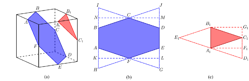
   Figure 1: The possible parameter space of $C_{i}^{r}$ in three dimensions. The box in Fig. 1 (a) gives the upper and the lower bounds of $C_{i}^{r}$ as Eq. (38). The blue and the red planes are two possible constraints of $C_{i}^{r}$ for a given set of $\widetilde{C}_{i}$ as Eq. (35), if the matrix $B$ is $1\times 3$ dimensional. All possible values of $C_{i}^{r}$ are in the blue/red convex polygon. The blue and the red convex polygons are laid flat in Figs. 1 (b) and 1 (c), respectively.

7. Using the estimates of $C_{i}^{r}$ obtained above, $L_{i}^{r}$ can be determined by method I.

This method to obtain $L_{i}^{r}$ and $C_{i}^{r}$ with the truncation errors is general. It is only based on the hypotheses in Sec. II. It does not depend on the number of observables, as long as the number of observables is larger than the number of $L_{i}^{r}$. In the present case, the number of observables (17) is small compared with the number of $C_{i}^{r}$ (38). Theoretically, if more observables are introduced, the values of $L_{i}^{r}$ are more precise. However, for $C_{i}^{r}$, besides giving more constraints of the existing $C_{i}^{r}$, the new observables may also introduce some new $C_{i}^{r}$. These new observables could also constrain the ranges of the new $C_{i}^{r}$. Sometimes, a new observable may give a new linearly independent $\widetilde{C}_{i}^{r}$. In this case, the rank of matrix $P$ in Eq. (34) increases. A new constraint should be introduced and $C_{i}^{r}$ could be constrained in some narrower ranges. Otherwise, if the rank of matrix $P$ is not changed, this new observable has a little impact on $C_{i}^{r}$. It only leads to a more precise set of $\widetilde{C}_{i}$.

VII The results by method II

The estimates and errors of $\widetilde{C}_{i}$ are given in the Table 4. If we randomly select a half of $\widetilde{C}_{i}$, the mean values and the standard deviations are unchanged. It indicates that the number of the samples is sufficient. Most of their relative errors are small enough, only $\Delta\widetilde{C}_{i}/\widetilde{C}_{i}\;(i=1,2,3,10)$ have large values. One could use this set of $\widetilde{C}_{i}$ to decide whether a part of $C_{i}^{r}$ are reasonable. A $\widetilde{C}_{i}$ is only related to a few $C_{i}^{r}$. For a particular research, sometimes it only needs a few $C_{i}^{r}$. If these $C_{i}^{r}$ are related to one or more $\widetilde{C}_{i}$, the values in Table 4 could decide to some extent whether these $C_{i}^{r}$ satisfy the observables discussed in this paper. If one knows more exact values of some $C_{i}^{r}$, some other $C_{i}^{r}$ can be obtained by these $\widetilde{C}_{i}^{r}$ too.

Table 4: The estimates and errors of $\widetilde{C}_{i}$.

$\widetilde{C}_{i}$	Values	$\widetilde{C}_{i}$	Values
$\widetilde{C}_{1}$	$0.02(12)$	$10\widetilde{C}_{10}$	$-0.06(13)$
$\widetilde{C}_{2}$	$0.19(34)$	$\widetilde{C}_{11}$	$0.24(02)$
$10^{2}\widetilde{C}_{3}$	$-0.72(42)$	$10^{3}\widetilde{C}_{12}$	$-0.18(01)$
$10^{2}\widetilde{C}_{4}$	$0.22(03)$	$10^{3}\widetilde{C}_{13}$	$1.02(44)$
$10\widetilde{C}_{5}$	$-0.16(02)$	$10^{4}\widetilde{C}_{14}$	$0.29(06)$
$10^{3}\widetilde{C}_{6}$	$0.26(13)$	$10^{3}\widetilde{C}_{15}$	$-0.11(01)$
$10^{2}\widetilde{C}_{7}$	$-0.42(12)$	$10^{4}\widetilde{C}_{16}$	$-0.56(06)$
$10\widetilde{C}_{8}$	$-0.45(09)$	$10^{4}\widetilde{C}_{17}$	$0.19(16)$
$10^{2}\widetilde{C}_{9}$	$-0.99(11)$

The distributions of $C_{i}^{r}$ are shown in Fig. 2 and Fig. 3. The upper and the lower boundaries in these figures are according to Eq. (38); their values are given in Table 9. They show that most $C_{i}^{r}$ are dependent on the initial boundaries. $C_{i}^{r}\,(i=1,3,7,8,18,66,69,88)$ are dependent on both sides of the boundaries, and $C_{i}^{r}\,(i=2,4,5,6,10,17,20,22,23,26,28,29,30,32,33,36,63,83,90)$ are dependent on one side. To obtain a more precise value, one needs more reasonable constraints or more inputs. Eleven $C_{i}^{r}\,(i=11,\ldots,16,19,21,25,31,34)$ are nearly boundary independent and are more reasonable. $C_{i}^{r}\,(i=11,12,13)$ are very special. There exists a jump in the center. We solve the linear programming problem [Eqs. (34) and (38)] and find that does not there exist any solution in the other side of the jump. This is because the other boundaries of $C_{i}^{r}$ limit the solution. However, the jump is far away from both boundaries. These LECs are also considered boundary independent.

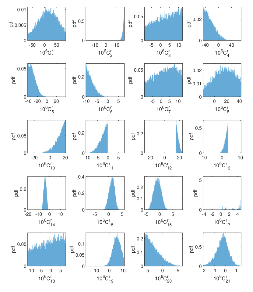
Figure 2: Distributions of the first part of $C_{i}^{r}$. The horizontal axis represents the value of $C_{i}^{r}$, the upper and the lower boundaries are given in Table 9. The vertical axis represents the probability density function (pdf).

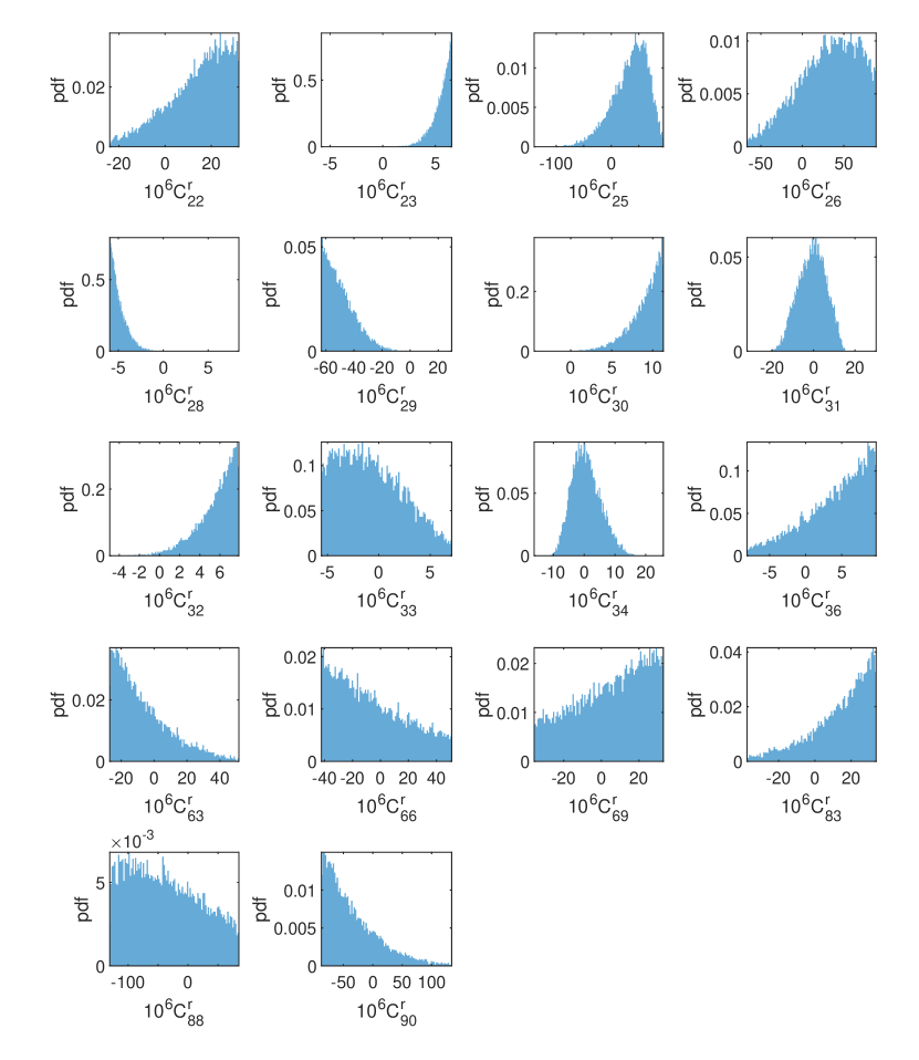
Figure 3: Distributions of the second part of $C_{i}^{r}$. The horizontal axis represents the value of $C_{i}^{r}$, the upper and the lower boundaries are given in Table 9. The vertical axis represents the probability density function (pdf).

The values of $C_{i}^{r}$ are shown in Table 5. Actually, in the calculation, the linear combinations $C^{r}_{63}-C^{r}_{83}+C^{r}_{88}/2$ and $C^{r}_{66}-C^{r}_{69}-C^{r}_{88}+C^{r}_{90}$ arise as a whole. We also present them in Table 5. Our initial ranges of $C_{i}^{r}$ are wide and many sets of $C_{i}^{r}$ can give a small $\chi^{2}/$d.o.f. Hence, their errors seem large. There is a high probability that the true values of $C_{i}^{r}$ are in these ranges, especially the boundary-independent ones. Some results in Ref. Bijnens and Ecker (2014) are marked with an asterisk, these values are very close to the original data on the website Bijnens (2019) (less than $10^{-10}$). We guess these results meet the fitting boundaries. The symbol “$\equiv 0$” in Column 4 and column 8 means these values are zeros in the large-$N_{c}$ limit. However, most intervals of $C_{i}^{r}\;(i=2,6,11,13,15,23)$ are far away from zero. It indicates that these LECs do not satisfy the large-$N_{c}$ limit. That is why the results in Ref. Jiang et al. (2015) can not fit $L_{i}^{r}$ well by method I.

Table 5: The values of $C_{i}^{r}$ in units of $10^{-6}$. The brackets “[” and “]” mean the results are dependent on the lower and the upper boundaries, respectively. The parentheses “(” and “)” mean the results are independent on the lower and the upper boundaries, respectively. The results with an asterisk mean the original data in the website Bijnens (2019) are very close to those in Ref. Bijnens and Ecker (2014) (less than $10^{-10}$). The symbol “$\equiv 0$” for the results in Ref. Jiang et al. (2015) means these values are zeros in the large-$N_{c}$ limits.

LECs	Results	Ref. Bijnens and Ecker (2014)	Ref. Jiang et al. (2015)	LECs	Results	Ref. Bijnens and Ecker (2014)	Ref. Jiang et al. (2015)
$C^{r}_{1}$	$14[37]$	12∗	$25.33^{+0.60}_{-1.11}$	$C^{r}_{22}$	$14(13]$	9.0∗	$-2.98^{+1.70}_{-2.21}$
$C^{r}_{2}$	$16(1]$	3.0∗	$\equiv 0$	$C^{r}_{23}$	$5.6(0.9]$	$-$1.0∗	$\equiv 0$
$C^{r}_{3}$	$2.9[6.0]$	4.0∗	$-0.43^{+0.09}_{-0.09}$	$C^{r}_{25}$	$34(33)$	$-$11∗	$-25.76^{-3.49}_{+5.02}$
$C^{r}_{4}$	$-26[16)$	15∗	$18.11^{+0.51}_{-0.85}$	$C^{r}_{26}$	$31(36]$	10	$23.04^{+2.98}_{-4.59}$
$C^{r}_{5}$	$-31[7)$	$-$4.0∗	$-10.88^{+0.85}_{-1.11}$	$C^{r}_{28}$	$-4.9[0.9)$	$-$2.0∗	$1.53^{+0.00}_{-0.09}$
$C^{r}_{6}$	$-7.9[1.8)$	$-$4.0∗	$\equiv 0$	$C^{r}_{29}$	$-49[11)$	$-$20∗	$-8.42^{-1.79}_{+2.04}$
$C^{r}_{7}$	$2.4[6.1]$	5.0∗	$\equiv 0$	$C^{r}_{30}$	$9.0(1.9]$	3.0∗	$3.15^{+0.09}_{-0.17}$
$C^{r}_{8}$	$15[16]$	19∗	$17.85^{-1.28}_{+1.36}$	$C^{r}_{31}$	$-0.71(6.70)$	2.0∗	$-3.91^{+0.60}_{-1.11}$
$C^{r}_{10}$	$13(6]$	$-$0.25	$-5.53^{+0.43}_{-0.51}$	$C^{r}_{32}$	$5.6(1.9]$	1.7	$1.45^{-0.17}_{+0.26}$
$C^{r}_{11}$	$-2.6(1.8)$	$-$4.0∗	$\equiv 0$	$C^{r}_{33}$	$-0.69[3.12)$	0.82	$-0.43^{-0.17}_{+0.43}$
$C^{r}_{12}$	$18(2)$	$-$2.8	$-2.89^{+0.09}_{-0.09}$	$C^{r}_{34}$	$0.68(4.67)$	7.0∗	$5.61^{-1.53}_{+2.47}$
$C^{r}_{13}$	$2.2(0.9)$	1.5	$\equiv 0$	$C^{r}_{36}$	$4.1(4.3]$	2.0∗	$\equiv 0$
$C^{r}_{14}$	$-4.2(1.2)$	$-$1.0∗	$-7.40^{+1.19}_{-1.79}$	$C^{r}_{63}$	$-6.6[16.8)$	–	$21.08^{-1.79}_{+2.13}$
$C^{r}_{15}$	$1.2(1.0)$	$-$3.0∗	$\equiv 0$	$C^{r}_{66}$	$-6.5[25.4]$	–	$6.80^{+0.34}_{-0.60}$
$C^{r}_{16}$	$-0.81(1.34)$	3.2	$\equiv 0$	$C^{r}_{69}$	$4.6[19.0]$	–	$4.42^{+0.00}_{-0.09}$
$C^{r}_{17}$	$3.6(1.6]$	$-$1.0∗	$1.45^{+0.09}_{-0.34}$	$C^{r}_{83}$	$14(16]$	–	$-14.79^{+1.45}_{-1.87}$
$C^{r}_{18}$	$-1.1[5.4]$	0.63	$-5.10^{+0.60}_{-0.77}$	$C^{r}_{88}$	$-38[59]$	–	$-14.37^{-5.78}_{+7.91}$
$C^{r}_{19}$	$5.3(2.8)$	$-$4.0∗	$-2.30^{+0.77}_{-1.11}$	$C^{r}_{90}$	$-35[44)$	–	$19.72^{-3.74}_{+4.68}$
$C^{r}_{20}$	$-2.9[2.3)$	1.0	$1.45^{-0.17}_{+0.26}$	$C^{r}_{63}-C^{r}_{83}+C^{r}_{88}/2$	$-39(33)$	$-$9.6	$28.69^{-6.13}_{+7.96}$
$C^{r}_{21}$	$-0.28(0.56)$	$-$0.48	$-0.51^{+0.09}_{-0.09}$	$C^{r}_{66}-C^{r}_{69}-C^{r}_{88}+C^{r}_{90}$	$-7.9(78.9)$	50	$36.47^{+2.38}_{-3.74}$

The second column in Table 6 lists the results for $L_{i}^{r}$. Compared with Ref. Bijnens and Ecker (2014), $\chi^{2}/\mathrm{d.o.f.}=4.3/9$ is closer to 1. It means that the constraints in Sec. VI relieve the overfitting problem. Convergences play an important role in the fit. For the normal distribution in Eq. (32), the initial standard deviation of ${L_{i}^{r}}=11.5\%$. Now, most relative deviations (in the third column) are obviously less than 11.5%, except for $L_{2,3}^{r}$. Their values are a little large. We consider they are also acceptable. $\mathrm{Pct}_{L_{2}^{r}}$ and $\mathrm{Pct}_{L_{3}^{r}}$ in the third column in Table 6 are larger than the others. The main reason is that a set of $L_{i}^{r}$ containing small $L_{2}^{r}$ (large $L_{3}^{r}$) are much easier to be picked out in the step ii (iv). For comparison, column 4 presents the average values of the remaining sets in step vi in Sec. VI, column 5 lists the relative deviations between column 4 and column 6. The values in column 2 and column 4 are close to each other. It seems that averaging $C_{i}^{r}$ or averaging $L_{i}^{r}$ first gives nearly no difference. These results are also not much different from fit 2 and the results in Ref. Bijnens and Ecker (2014). Because the results in column 2 are related to $C_{i}^{r}$ in Table 5, we choose them as our $L_{i}^{r}$ results.

Table 6: The results for $L_{i}^{r}$. The second column is the final results of $L_{i}^{r}$. The fourth column is only a simple average of the value in step vi in Sec. VI. $\mathrm{Pct}_{L_{i}^{r}}$ in the second and the fourth column is defined in Eq. (31).

$L_{i}^{r}$	Results	$\mathrm{Pct}_{L_{i}^{r}}(\%)$	Average	$\mathrm{Pct}_{L_{i}^{r}}(\%)$	Fit 2	Ref. Bijnens and Ecker (2014) fit $p^{6}$
$10^{3}L_{1}^{r}$	$0.43(05)$	2.2	$0.44(05)$	0.8	0.44(05)	0.53(06)
$10^{3}L_{2}^{r}$	$0.74(04)$	14.0	$0.77(05)$	10.2	0.84(10)	0.81(04)
$10^{3}L_{3}^{r}$	$-2.47(17)$	15.0	$-2.55(15)$	11.6	$-$2.84(16)	$-$3.07(20)
$10^{3}L_{4}^{r}$	$0.33(08)$	9.3	$0.30(03)$	2.2	0.30(33)	$\equiv$0.3
$10^{3}L_{5}^{r}$	$0.95(04)$	2.6	$0.95(09)$	2.9	0.92(02)	1.01(06)
$10^{3}L_{6}^{r}$	$0.20(03)$	9.9	$0.21(02)$	8.8	0.22(08)	0.14(05)
$10^{3}L_{7}^{r}$	$-0.23(08)$	2.2	$-0.23(03)$	1.7	$-$0.23(12)	$-$0.34(09)
$10^{3}L_{8}^{r}$	$0.42(09)$	5.4	$0.42(04)$	4.7	0.44(10)	0.47(10)
$\chi^{2}$(d.o.f.)	4.3(9)	–	–	–	4.2(4)	1.0(10)

In Table 7, the values of the observables at each order and $\mathrm{Pct}_{\mathrm{order}}$ are listed. It can be seen that most observables have good convergence, except $a_{0}^{1/2}$ and $a_{0}^{3/2}$ at NNLO. The reason has been discussed in Sec. V.1 and step iv in Sec. VI. Whether the higher-order values are really small or not requires a more reasonable analysis. It is beyond this work. The truncation errors in the fifth column are very small, all $\mathrm{Pct}_{\mathrm{HO}}$ are less than 4%, except $l_{2}^{r}$. However, the absolute value of $l_{2}^{r}$ decreases order by order. It is not a contradiction. Now, with the hypothesises in Sec. II, the first three problems in the Introduction are solved, and the cause of the last two problems is also found.

Table 7: The convergence of observables. The second to the fifth columns give the contributions and $\mathrm{Pct}_{\mathrm{order}}$ at each order. The theoretical values are given in the sixth column. The experimental values (inputs) are listed in the last column. $\bar{l}_{i}$ have been changed to $l_{i}^{r}$.

physical quantities	LO$|\mathrm{Pct}_{\mathrm{LO}}$(%)	NLO$|\mathrm{Pct}_{\mathrm{NLO}}$(%)	NNLO$|\mathrm{Pct}_{\mathrm{NNLO}}$(%)	HO$|\mathrm{Pct}_{\mathrm{HO}}$(%)	Theory	Inputs
$m_{s}/\hat{m}|_{1}$	$25.8(94.8)$	$2.0(7.2)$	$-1.1(4.0)$	$0.6(2.0)$	$27.3$	$27.3_{-1.3}^{+0.7}$
$m_{s}/\hat{m}|_{2}$	$24.2(88.7)$	$3.3(12.2)$	$-0.8(2.8)$	$0.5(1.9)$	$27.3$	$27.3_{-1.3}^{+0.7}$
$F_{K}/F_{\pi}$	$1.000(83.4)$	$0.169(14.1)$	$0.023(1.9)$	$0.007(0.6)$	$1.199$	$1.199\pm 0.003$
$f_{s}$	$3.782(66.2)$	$1.322(23.1)$	$0.371(6.5)$	$0.235(4.1)$	$5.709$	$5.712\pm 0.032$
$g_{p}$	$3.782(76.7)$	$0.776(15.7)$	$0.366(7.4)$	$0.007(0.1)$	$4.931$	$4.958\pm 0.085$
$a_{0}^{0}$	$0.1592(72.5)$	$0.0453(20.6)$	$0.0098(4.5)$	$0.0053(2.4)$	$0.2196$	$0.2196\pm 0.0034$
$10a_{0}^{2}$	$-0.455(103.8)$	$0.022(5.0)$	$-0.010(2.2)$	$0.005(1.1)$	$-0.438$	$-0.444\pm 0.012$
$a_{0}^{1/2}m_{\pi}$	$0.142(62.6)$	$0.033(14.6)$	$0.049(21.7)$	$0.002(1.0)$	$0.226$	$0.224\pm 0.022$
$10a_{0}^{3/2}m_{\pi}$	$-0.709(150.2)$	$0.094(19.8)$	$0.142(30.1)$	$0.001(0.3)$	$-0.472$	$-0.448\pm 0.077$
$F_{S}^{\pi}(0)/2B_{0}$	$1.000(98.1)$	$0.019(1.9)$	$0.000(0.0)$	$0.000(0.0)$	$1.019$	–
$10^{3}l_{1}^{r}$	–	$-3.2(81.5)$	$-0.6(15.1)$	$-0.1(3.4)$	$-4.0$	$-4.0\pm 0.6$
$10^{3}l_{2}^{r}$	–	$3.0(145.6)$	$-1.3(66.5)$	$0.4(20.8)$	$2.0$	$1.9\pm 0.2$
$10^{3}l_{3}^{r}$	–	$0.2(102.5)$	$-0.0(2.6)$	$0.0(0.1)$	$0.2$	$0.3\pm 1.1$
$10^{3}l_{4}^{r}$	–	$6.3(96.8)$	$0.2(3.1)$	$0.0(0.1)$	$6.6$	$6.2\pm 1.3$

VIII summary and discussion

In this paper, we have computed the NLO and the NNLO LECs for pseudoscalar mesons with a new method (method II). The results are present in Table 6 and Table 5, respectively. The truncation errors are considered in the computation with some hypotheses in Sec. II; i.e., the theoretical values of observables are satisfied with the convergence in ChPT, all $L_{i}^{r}$ are stable and $C_{i}^{r}$ are consistent with those in the other references. The results nearly satisfy all these hypotheses, and all random processes are repeated several times. The results are nearly unchanged. They are reasonable in statistics. Some linear combinations of $C_{i}^{r}$ called $\widetilde{C}_{i}^{r}$ are also given. Their relative errors are less than $C_{i}^{r}$ and their values are more reliable. If one knows more exact values of some $C_{i}^{r}$, some other $C_{i}^{r}$ can be obtained by these $\widetilde{C}_{i}^{r}$.

First, a modified global fit method is used to obtain $L_{i}^{r}$. If they are only fitted at NLO, the results are very close to the NNLO fitted results in Ref. Bijnens and Ecker (2014). It indicates that the higher-order estimates have a good prediction. The estimation is reasonable. However, some $L_{i}^{r}$ deviate from the NLO fitting ones in Ref. Bijnens and Ecker (2014) too much. The main reason is that the higher-order estimates of $f_{s}$, $g_{p}$, $a_{0}^{0}$ and $a_{0}^{1/2}$ are not very small; i.e., the truncation errors can make a great impact on the values of the lower order LECs. The $\pi K$ scattering lengths $a_{0}^{1/2}$ and $a_{0}^{3/2}$ can not be fitted well, because their LO contributions can not give a good prediction, and the NLO contributions tend to be small. For the NLO fit, all the theoretical values of observables have good convergence. However, at NNLO, we have tried two sets of $C_{i}^{r}$ in the references, but the results are not very good.

Later, we use a new method to obtain both $L_{i}^{r}$ and $C_{i}^{r}$. The idea is that the linearly independent combinations of $C_{i}^{r}$ ($\widetilde{C}_{i}$) are obtained first, and then $C_{i}^{r}$ are estimated with the Monte-Carlo method. Finally, $L_{i}^{r}$ are fitted by these $C_{i}^{r}$. Some $C_{i}^{r}$ are dependent on the initial boundaries. In order to obtain more precise values, these $C_{i}^{r}$ need more information to narrow the boundaries. The other $C_{i}^{r}$ are boundary independent and can be limited to some reliable intervals. The relative errors between the NLO fitting results and the one by this method are all small. All observables have good convergence, except $a_{0}^{1/2}$ and $a_{0}^{3/2}$. For $a_{0}^{1/2}$ and $a_{0}^{3/2}$, we assume that their contributions beyond NNLO are small and their NNLO contributions are large, because their NLO values are not large enough. Whether this assumption is correct or not needs a more reasonable estimate beyond the NNLO according to ChPT.

Some constraints in this paper are very weak, such as Eqs. (32), (33), (36), (38), and (39), because we want to cover the true value as far as possible. Hence, some error ranges of the NNLO LECs are large. If another method can introduce more restrictive constraints, their error ranges may be narrower. However, the values of $L_{i}^{r}$ are more reliable. Their NLO and NNLO fitting results are very closed. One could use these $L_{i}^{r}$ for further calculations directly. However, the ranges of $C_{i}^{r}$ are larger. They could only give rough estimates at NNLO. The estimates could be treated as references to judge whether the NNLO contributions are small or large. We hope that this new method not only determines the LECs in ChPT for mesons, but it will also generalize to ChPT for baryons and another effective field theory in the future. Other effective field theories should also contain a lot of LECs, especially at the high order. If one fits the low-order LECs, the fit at the low order should also give a reliable set of LECs with truncation errors, even without the higher calculations. It would save a lot of effort. Some new predictions could be given with these fitting LECs. Some choices in this paper are also personal favorites. For example, the three hypotheses in Sec. II are very rough, for some special cases, stricter or looser conditions might be introduced. We also choose uniform distribution in Eq. (32), but the strict distribution would be very complex. These need to be further studied in the future too.

IX acknowledgements

We thank Professor Johan Bijnens for some help with $K_{\ell 4}$ program. We also thank Dr. Da-Bin Lin for providing a powerful computer. Yang and Jiang thank Dr. Sarah Wesolowski for giving a lot of helpful comments. This work was supported by the National Science Foundation of China (NSFC) under Grant No. 11565004, Guangxi Science Foundation under Grants No. 2018GXNSFAA281180 and No. 2017AD22006, and the high-performance computing platform of Guangxi University.

Appendix A The linear combinations of $C_{i}^{r}$

In Sec. VI, most $C_{i}^{r}$ have not been calculated separately, because the number of redundant parameters is very large. In this appendix, some $\widetilde{C}_{i}$ will be defined. They are linear combinations of $C_{i}^{r}$. These $\widetilde{C}_{i}$ can be calculated separately.

Generally, the NNLO contribution of some observables $X_{j}$ can be separated into two parts, one part is proportional to $C_{i}^{r}$ ($X_{j,C}$) and the other part is related to $L_{i}^{r}$ ($X_{j,L}$)

$$X_{j}=X_{j,L}+X_{j,C}=X_{j,L}+d_{j}A_{j},$$ (40)

where different $j$ denotes different observables which will be discussed below, $d_{j}$ are possible dimensional parameters, and $A_{j}$ are dimensionless coefficients. $d_{j}$ are independent of $C_{i}^{r}$, but $A_{j}$ are dependent on $C_{i}^{r}$. In this section, the discussion is only about $X_{j,C}$, so we will not go into detail below.

For meson masses and decay constants, $j=1\ldots 5$ denote $m_{\pi}^{2},m_{K}^{2},m_{\eta}^{2},F_{\pi}/F_{0},F_{K}/F_{0}$, respectively; $d_{1,2,3}=m_{\pi}^{6}/F_{\pi}^{4}$, $d_{4,5}=m_{\pi}^{4}/F_{\pi}^{4}$ and $A_{j}$ are

$$A_{1}= 48\,C^{r}_{19}-16\,C^{r}_{14}-16\,C^{r}_{17}-32\,C^{r}_{12}+32\,C^{r}_{31}-C^{r}_{15}\,\left(32\,a^{2}+16\right)-C^{r}_{13}\,\left(64\,a^{2}+32\right)$$

$$+C^{r}_{32}\,\left(64\,a^{2}+32\right)+C^{r}_{20}\,\left(64\,a^{4}+80\right)-C^{r}_{16}\,\left(64\,a^{4}-64\,a^{2}+48\right)+48\,C^{r}_{21}\,{\left(2\,a^{2}+1\right)}^{2},$$ (41)

$$A_{2}= 32\,C^{r}_{31}\,a^{6}-32\,C^{r}_{12}\,a^{6}-16\,C^{r}_{14}\,a^{2}\,\left(2\,a^{4}-2\,a^{2}+1\right)+48\,C^{r}_{19}\,a^{2}\,\left(2\,a^{4}-2\,a^{2}+1\right)$$

$$-16\,C^{r}_{16}\,a^{2}\,\left(4\,a^{4}-4\,a^{2}+3\right)+16\,C^{r}_{20}\,a^{2}\,\left(8\,a^{4}-2\,a^{2}+3\right)+48\,C^{r}_{21}\,a^{2}\,{\left(2\,a^{2}+1\right)}^{2}$$

$$-32\,C^{r}_{13}\,a^{4}\,\left(2\,a^{2}+1\right)-16\,C^{r}_{15}\,a^{4}\,\left(2\,a^{2}+1\right)-16\,C^{r}_{17}\,a^{2}\,\left(2\,a^{2}-1\right)+32\,C^{r}_{32}\,a^{4}\,\left(2\,a^{2}+1\right),$$ (42)

$$A_{3}= C^{r}_{20}\,\left(256\,a^{6}-192\,a^{4}+64\,a^{2}+16\right)+C^{r}_{19}\,\left(256\,a^{6}-384\,a^{4}+192\,a^{2}-16\right)$$

$$-C^{r}_{16}\,\left(\frac{256\,a^{6}}{3}-\frac{320\,a^{4}}{3}+\frac{256\,a^{2}}{3}-16\right)-C^{r}_{32}\,\left(-\frac{512\,a^{6}}{3}+\frac{256\,a^{4}}{3}+\frac{64\,a^{2}}{3}-32\right)$$

$$+C^{r}_{31}\,\left(\frac{512\,a^{6}}{3}-256\,a^{4}+128\,a^{2}-\frac{32}{3}\right)-C^{r}_{14}\,\left(\frac{512\,a^{6}}{9}-\frac{640\,a^{4}}{9}+\frac{320\,a^{2}}{9}-\frac{16}{3}\right)$$

$$-C^{r}_{17}\,\left(\frac{512\,a^{6}}{9}-\frac{640\,a^{4}}{9}+\frac{320\,a^{2}}{9}-\frac{16}{3}\right)-\frac{32\,C^{r}_{12}\,{\left(4\,a^{2}-1\right)}^{3}}{27}$$

$$-\frac{32\,C^{r}_{13}\,\left(2\,a^{2}+1\right)\,{\left(4\,a^{2}-1\right)}^{2}}{9}-\frac{16\,C^{r}_{15}\,\left(2\,a^{2}+1\right)\,{\left(4\,a^{2}-1\right)}^{2}}{9}$$

$$+16\,C^{r}_{21}\,{\left(2\,a^{2}+1\right)}^{2}\,\left(4\,a^{2}-1\right)-\frac{128\,C^{r}_{18}\,{\left(a^{2}-1\right)}^{2}\,\left(4\,a^{2}-1\right)}{9}+\frac{512\,C^{r}_{33}\,a^{2}\,{\left(a^{2}-1\right)}^{2}}{3},$$ (43)

$$A_{4}= 8\,C^{r}_{14}+8\,C^{r}_{17}+C^{r}_{15}\,\left(16\,a^{2}+8\right)+C^{r}_{16}\,\left(32\,a^{4}-32\,a^{2}+24\right),$$ (44)

$$A_{5}= C^{r}_{17}\,\left(16\,a^{2}-8\right)+C^{r}_{14}\,\left(16\,a^{4}-16\,a^{2}+8\right)+C^{r}_{16}\,\left(32\,a^{4}-32\,a^{2}+24\right)+8\,C^{r}_{15}\,a^{2}\,\left(2\,a^{2}+1\right),$$ (45)

where $a=m_{K}/m_{\pi}$. For $m_{s}/\hat{m}|_{1}$, $m_{s}/\hat{m}|_{2}$ and $F_{K}/F_{\pi}$, the NNLO order contributions related to $C_{i}^{r}$ are $(m_{\pi}^{4}/F_{\pi}^{4})\widetilde{C}_{i}$ $(i=1,2,3)$ respectively, where

$$\widetilde{C}_{1}= \frac{m_{K}^{2}}{m_{\pi}^{2}}A_{1}-A_{2},$$ (46)

$$\widetilde{C}_{2}= \frac{m_{\eta}^{2}}{m_{\pi}^{2}}A_{1}-A_{3},$$ (47)

$$\widetilde{C}_{3}= A_{5}-A_{4}.$$ (48)

For $K_{\ell 4}$ form factors, the NNLO contributions of $f_{s}$ and $f_{s}^{\prime}$ can be written as Amorós et al. (2000a)

$$F(s_{\pi},s_{\ell}=0,\cos\theta=0)_{6}=F_{6,L}+F_{6,C}=F_{6,L}+\frac{1}{F_{\pi}^{4}}(A_{6}s_{\pi}^{2}+A_{7}s_{\pi}m_{\pi}^{2}+A_{8}m_{\pi}^{4}).$$ (49)

$$A_{6}= 4\,C^{r}_{3}-64\,C^{r}_{2}-14\,C^{r}_{1}+20\,C^{r}_{4},$$ (50)

$$A_{7}= C^{r}_{10}\,\left(4\,a^{2}+4\right)+C^{r}_{5}\,\left(4\,a^{2}+16\right)+C^{r}_{8}\,\left(16\,a^{2}+4\right)+C^{r}_{12}\,\left(12\,a^{2}-8\right)$$

$$+C^{r}_{22}\,\left(4\,a^{2}+8\right)+C^{r}_{11}\,\left(16\,a^{2}+8\right)+C^{r}_{4}\,\left(4\,a^{2}-32\right)-C^{r}_{23}\,\left(8\,a^{2}+16\right)$$

$$+C^{r}_{25}\,\left(8\,a^{2}+16\right)+C^{r}_{1}\,\left(10\,a^{2}+48\right)+C^{r}_{6}\,\left(40\,a^{2}+20\right)+C^{r}_{7}\,\left(32\,a^{2}+32\right)$$

$$+C^{r}_{13}\,\left(48\,a^{2}-40\right)+C^{r}_{2}\,\left(32\,a^{2}+192\right)+4\,C^{r}_{3}\,a^{2},$$ (51)

$$A_{8}= 128\,C^{r}_{16}+128\,C^{r}_{28}+C^{r}_{5}\,\left(4\,a^{4}-32\right)-C^{r}_{1}\,\left(16\,a^{2}+32\right)-C^{r}_{14}\,\left(16\,a^{2}-32\right)$$

$$-C^{r}_{26}\,\left(16\,a^{2}-32\right)+C^{r}_{15}\,\left(80\,a^{2}+8\right)+C^{r}_{17}\,\left(64\,a^{2}-48\right)-C^{r}_{7}\,\left(64\,a^{2}+64\right)$$

$$-C^{r}_{2}\,\left(64\,a^{2}+128\right)-C^{r}_{6}\,\left(-8\,a^{4}+60\,a^{2}+32\right)-C^{r}_{12}\,\left(12\,a^{4}-24\,a^{2}+64\right)$$

$$-C^{r}_{13}\,\left(16\,a^{4}+72\,a^{2}+64\right)-28\,C^{r}_{8}\,a^{2}-16\,C^{r}_{25}\,a^{2}-32\,C^{r}_{29}\,a^{2}-64\,C^{r}_{30}\,a^{2}$$

$$-8\,C^{r}_{34}\,a^{4}-32\,C^{r}_{36}\,a^{2}+4\,C^{r}_{10}\,a^{2}\,\left(a^{2}+1\right)+8\,C^{r}_{23}\,a^{2}\,\left(a^{2}-2\right)+4\,C^{r}_{22}\,a^{2}\,\left(a^{2}-6\right)$$

$$+8\,C^{r}_{11}\,a^{2}\,\left(2\,a^{2}+1\right).$$ (52)

$f^{\prime}_{s}$ can be calculated numerically

$$f^{\prime}_{s}=4m_{\pi}^{2}\frac{F(s^{\prime}_{\pi})-F(s_{\pi})}{s^{\prime}_{\pi}-s_{\pi}},$$ (53)

where $s_{\pi}=(2m_{\pi}+0.001\mathrm{MeV})^{2}$ and $s^{\prime}_{\pi}=(293\mathrm{MeV})^{2}$ are around the threshold. The two observables $f_{s}$ and $f^{\prime}_{s}$ are related to two independent linear combinations

$$\widetilde{C}_{4} =A_{6}-\frac{m_{\pi}^{4}}{s_{\pi}s^{\prime}_{\pi}}A_{8},$$ (54)

$$\widetilde{C}_{5} =A_{7}+\frac{m_{\pi}^{2}(s_{\pi}+s^{\prime}_{\pi})}{s_{\pi}s^{\prime}_{\pi}}A_{8}.$$ (55)

The discussion for $g_{p}$ and $g^{\prime}_{p}$ is similar to $f_{s}$ and $f_{s}^{\prime}$. The parameters $A_{9,10,11}$ and the independent linear combinations $\widetilde{C}_{6,7}$ are

$$A_{9}= 4\,C^{r}_{3}-2\,C^{r}_{1}+2\,C^{r}_{4}+3\,C^{r}_{66}-3\,C^{r}_{69}-3\,C^{r}_{88}+3\,C^{r}_{90},$$ (56)

$$A_{10}= C^{r}_{10}\,\left(4\,a^{2}+4\right)-C^{r}_{6}\,\left(8\,a^{2}+4\right)-4\,C^{r}_{8}-C^{r}_{4}\,\left(8\,a^{2}+8\right)-C^{r}_{12}\,\left(4\,a^{2}+16\right)$$

$$+C^{r}_{22}\,\left(8\,a^{2}+4\right)+C^{r}_{11}\,\left(16\,a^{2}+8\right)-C^{r}_{25}\,\left(8\,a^{2}+4\right)+C^{r}_{63}\,\left(4\,a^{2}-4\right)$$

$$-C^{r}_{66}\,\left(2\,a^{2}+4\right)+C^{r}_{69}\,\left(2\,a^{2}+4\right)-C^{r}_{13}\,\left(48\,a^{2}+24\right)-C^{r}_{83}\,\left(4\,a^{2}-4\right)$$

$$+C^{r}_{88}\,\left(4\,a^{2}+2\right)-C^{r}_{90}\,\left(2\,a^{2}+4\right)-2\,C^{r}_{1}\,a^{2}+4\,C^{r}_{3}\,a^{2}-4\,C^{r}_{5}\,a^{2},$$ (57)

$$A_{11}= 16\,C^{r}_{17}+C^{r}_{15}\,\left(16\,a^{2}+8\right)+C^{r}_{66}\,\left(4\,a^{2}-a^{4}\right)+C^{r}_{90}\,\left(4\,a^{2}-a^{4}\right)-4\,C^{r}_{5}\,a^{4}-4\,C^{r}_{8}\,a^{2}$$

$$-28\,C^{r}_{12}\,a^{4}+16\,C^{r}_{14}\,a^{2}-20\,C^{r}_{22}\,a^{2}+20\,C^{r}_{25}\,a^{2}+16\,C^{r}_{26}\,a^{2}-32\,C^{r}_{29}\,a^{2}-8\,C^{r}_{34}\,a^{4}$$

$$-C^{r}_{88}\,\left(a^{4}+2\,a^{2}\right)-2\,C^{r}_{4}\,a^{2}\,\left(a^{2}-4\right)+4\,C^{r}_{10}\,a^{2}\,\left(a^{2}+1\right)-4\,C^{r}_{63}\,a^{2}\,\left(a^{2}-1\right)$$

$$+C^{r}_{69}\,a^{2}\,\left(a^{2}-4\right)+4\,C^{r}_{83}\,a^{2}\,\left(a^{2}-1\right)-4\,C^{r}_{6}\,a^{2}\,\left(2\,a^{2}+1\right)+8\,C^{r}_{11}\,a^{2}\,\left(2\,a^{2}+1\right)$$

$$-24\,C^{r}_{13}\,a^{2}\,\left(2\,a^{2}+1\right).$$ (58)

$$\widetilde{C}_{6}= A_{9}-\frac{m_{\pi}^{4}}{s_{\pi}s^{\prime}_{\pi}}A_{11},$$ (59)

$$\widetilde{C}_{7}= A_{10}+\frac{m_{\pi}^{2}(s_{\pi}+s^{\prime}_{\pi})}{s_{\pi}s^{\prime}_{\pi}}A_{11}.$$ (60)

The NNLO contribution of the $\pi\pi$ scattering amplitude is related to $A(s,t,u)$ and $A(t,u,s)=A(u,s,t)$, where $s=4m_{\pi}^{2}$, $t=0$ and $u=0$. They can be written as Eq. (40) Bijnens et al. (2004a),

$$A_{12}= 192\,C^{r}_{3}-128\,C^{r}_{2}-64\,C^{r}_{1}+384\,C^{r}_{4}+32\,C^{r}_{5}+64\,C^{r}_{7}+32\,C^{r}_{8}+32\,C^{r}_{10}-96\,C^{r}_{12}$$

$$+64\,C^{r}_{14}+128\,C^{r}_{16}+64\,C^{r}_{17}+96\,C^{r}_{19}-128\,C^{r}_{22}-128\,C^{r}_{23}+192\,C^{r}_{25}+64\,C^{r}_{26}$$

$$+128\,C^{r}_{28}-192\,C^{r}_{29}-128\,C^{r}_{30}+96\,C^{r}_{31}+C^{r}_{6}\,\left(64\,a^{2}+32\right)+C^{r}_{11}\,\left(64\,a^{2}+32\right)$$

$$+C^{r}_{15}\,\left(64\,a^{2}+96\right)-C^{r}_{13}\,\left(64\,a^{2}+160\right)+C^{r}_{20}\,\left(64\,a^{2}+160\right)+C^{r}_{32}\,\left(64\,a^{2}+160\right)$$

$$+C^{r}_{21}\,\left(384\,a^{2}+192\right),$$ (61)

$$A_{13}= 64\,C^{r}_{1}+128\,C^{r}_{2}-64\,C^{r}_{3}-128\,C^{r}_{4}+32\,C^{r}_{5}+64\,C^{r}_{7}+32\,C^{r}_{8}+32\,C^{r}_{10}-96\,C^{r}_{12}$$

$$-64\,C^{r}_{14}-128\,C^{r}_{16}-64\,C^{r}_{17}+96\,C^{r}_{19}+128\,C^{r}_{22}+128\,C^{r}_{23}-64\,C^{r}_{25}-64\,C^{r}_{26}$$

$$-128\,C^{r}_{28}+64\,C^{r}_{29}+96\,C^{r}_{31}+C^{r}_{6}\,\left(64\,a^{2}+32\right)+C^{r}_{11}\,\left(64\,a^{2}+32\right)$$

$$-C^{r}_{15}\,\left(64\,a^{2}+96\right)-C^{r}_{13}\,\left(64\,a^{2}+160\right)+C^{r}_{20}\,\left(64\,a^{2}+160\right)+C^{r}_{32}\,\left(64\,a^{2}+160\right)$$

$$+C^{r}_{21}\,\left(384\,a^{2}+192\right).$$ (62)

and $d_{12,13}=m_{\pi}^{6}/F_{\pi}^{6}$. The scattering lengths $a_{0}^{0}$ and $a_{0}^{2}$ are related to $m_{\pi}^{6}\widetilde{C}_{8,9}/(32\pi F_{\pi}^{6})$, respectively, where

$$\widetilde{C}_{8}= 3A_{12}+2A_{13},$$ (63)

$$\widetilde{C}_{9}= A_{13}.$$ (64)

For $\pi K$ scattering, the NNLO contribution is related to $T^{\frac{3}{2}}(s,t,u)$ and $T^{\frac{3}{2}}(u,t,s)$, where $s=(m_{K}+m_{\pi})^{2}$, $t=0$, and $u=(m_{K}-m_{\pi})^{2}$. They can be written as Eq. (40) Bijnens et al. (2004b),

$$A_{14}= 64\,C^{r}_{29}\,a^{3}-128\,C^{r}_{4}\,a^{3}-64\,C^{r}_{25}\,a^{3}-64\,C^{r}_{3}\,a^{3}-32\,C^{r}_{14}\,a^{2}\,\left(a+1\right)$$

$$-32\,C^{r}_{17}\,a\,\left(a^{3}+1\right)-16\,C^{r}_{15}\,a\,\left(4\,a^{3}+2\,a^{2}+3\,a+1\right)+16\,C^{r}_{1}\,a^{2}\,{\left(a+1\right)}^{2}$$

$$+64\,C^{r}_{2}\,a^{2}\,\left(a^{2}+1\right)+16\,C^{r}_{5}\,a^{2}\,\left(a^{2}+1\right)+32\,C^{r}_{7}\,a^{2}\,\left(a^{2}+1\right)+16\,C^{r}_{8}\,a^{2}\,\left(a^{2}+1\right)$$

$$+16\,C^{r}_{10}\,a^{2}\,\left(a^{2}+1\right)-48\,C^{r}_{12}\,a^{2}\,\left(a^{2}+1\right)-64\,C^{r}_{16}\,a^{2}\,\left(a^{2}+1\right)$$

$$+48\,C^{r}_{19}\,a^{2}\,\left(a^{2}+1\right)+32\,C^{r}_{22}\,a^{2}\,{\left(a+1\right)}^{2}+64\,C^{r}_{23}\,a^{2}\,\left(a^{2}+1\right)-16\,C^{r}_{26}\,a^{2}\,{\left(a+1\right)}^{2}$$

$$-64\,C^{r}_{28}\,a^{2}\,\left(a^{2}+1\right)+48\,C^{r}_{31}\,a^{2}\,\left(a^{2}+1\right)+32\,C^{r}_{6}\,a^{2}\,\left(2\,a^{2}+1\right)$$

$$+32\,C^{r}_{11}\,a^{2}\,\left(2\,a^{2}+1\right)-32\,C^{r}_{13}\,a^{2}\,\left(4\,a^{2}+3\right)+192\,C^{r}_{21}\,a^{2}\,\left(2\,a^{2}+1\right)$$

$$+32\,C^{r}_{20}\,a^{2}\,\left(4\,a^{2}+3\right)+32\,C^{r}_{32}\,a^{2}\,\left(4\,a^{2}+3\right),$$ (65)

$$A_{15}= 64\,C^{r}_{3}\,a^{3}+128\,C^{r}_{4}\,a^{3}+64\,C^{r}_{25}\,a^{3}-64\,C^{r}_{29}\,a^{3}+32\,C^{r}_{14}\,a^{2}\,\left(a-1\right)$$

$$-32\,C^{r}_{17}\,a\,\left(a^{3}-1\right)-16\,C^{r}_{15}\,a\,\left(4\,a^{3}-2\,a^{2}+3\,a-1\right)+16\,C^{r}_{1}\,a^{2}\,{\left(a-1\right)}^{2}$$

$$+64\,C^{r}_{2}\,a^{2}\,\left(a^{2}+1\right)+16\,C^{r}_{5}\,a^{2}\,\left(a^{2}+1\right)+32\,C^{r}_{7}\,a^{2}\,\left(a^{2}+1\right)+16\,C^{r}_{8}\,a^{2}\,\left(a^{2}+1\right)$$

$$+16\,C^{r}_{10}\,a^{2}\,\left(a^{2}+1\right)-48\,C^{r}_{12}\,a^{2}\,\left(a^{2}+1\right)-64\,C^{r}_{16}\,a^{2}\,\left(a^{2}+1\right)$$

$$+48\,C^{r}_{19}\,a^{2}\,\left(a^{2}+1\right)+32\,C^{r}_{22}\,a^{2}\,{\left(a-1\right)}^{2}+64\,C^{r}_{23}\,a^{2}\,\left(a^{2}+1\right)-16\,C^{r}_{26}\,a^{2}\,{\left(a-1\right)}^{2}$$

$$-64\,C^{r}_{28}\,a^{2}\,\left(a^{2}+1\right)+48\,C^{r}_{31}\,a^{2}\,\left(a^{2}+1\right)+32\,C^{r}_{6}\,a^{2}\,\left(2\,a^{2}+1\right)$$

$$+32\,C^{r}_{11}\,a^{2}\,\left(2\,a^{2}+1\right)-32\,C^{r}_{13}\,a^{2}\,\left(4\,a^{2}+3\right)+192\,C^{r}_{21}\,a^{2}\,\left(2\,a^{2}+1\right)$$

$$+32\,C^{r}_{20}\,a^{2}\,\left(4\,a^{2}+3\right)+32\,C^{r}_{32}\,a^{2}\,\left(4\,a^{2}+3\right),$$ (66)

where $d_{14,15}=m_{\pi}^{6}/F_{\pi}^{6}$. The scattering lengths $a_{0}^{1/2}$ and $a_{0}^{3/2}$ are related to $m_{\pi}^{6}\widetilde{C}_{10,11}/(8\pi F_{\pi}^{6}\sqrt{s})$, respectively, where

$$\widetilde{C}_{10}= -\frac{1}{2}A_{14}+\frac{3}{2}A_{15},$$ (67)

$$\widetilde{C}_{11}= A_{14}.$$ (68)

For the pion scalar form factor $F_{S}^{\pi}(t)$, the NNLO contribution is Bijnens and Dhonte (2003)

$$\Big{(}\frac{F_{S}^{\pi}(t)}{2B_{0}}\Big{)}_{6}= \Big{(}\frac{F_{S}^{\pi}(t)}{2B_{0}}\Big{)}_{6,L}+\frac{1}{F_{\pi}^{4}}(A_{16}t^{2}+A_{17}tm_{\pi}^{2}+A_{18}m_{\pi}^{4}),$$ (69)

$$A_{16}= -8\,C^{r}_{12}-16\,C^{r}_{13},$$ (70)

$$A_{17}= 32\,C^{r}_{12}+64\,C^{r}_{13}+16\,C^{r}_{14}+32\,C^{r}_{16}+16\,C^{r}_{17}+16\,C^{r}_{34}+16\,C^{r}_{36}+C^{r}_{15}\,\left(16\,a^{2}+24\right),$$ (71)

$$A_{18}= 144\,C^{r}_{19}-48\,C^{r}_{14}-48\,C^{r}_{17}-96\,C^{r}_{12}+96\,C^{r}_{31}-C^{r}_{15}\,\left(64\,a^{2}+64\right)$$

$$-C^{r}_{13}\,\left(128\,a^{2}+128\right)+C^{r}_{32}\,\left(128\,a^{2}+128\right)-C^{r}_{16}\,\left(64\,a^{4}-64\,a^{2}+112\right)$$

$$+C^{r}_{20}\,\left(64\,a^{4}+64\,a^{2}+240\right)+C^{r}_{21}\,\left(192\,a^{4}+576\,a^{2}+240\right).$$ (72)

$\langle r^{2}\rangle_{S}^{\pi}$ and $c_{S}^{\pi}$ are related to $\widetilde{C}_{12}=A_{16}$ and $\widetilde{C}_{13}=A_{17}$, respectively.

Reference Gasser et al. (2007) gives the relations between $l_{i}^{r}$ and $L_{i}^{r}$ up to the NNLO. The NNLO contributions related to $C_{i}^{r}$ are $l_{i}^{r}\sim M_{K}^{2}\widetilde{C}_{i+13}/(16\pi^{2}F_{0}^{2}),(i=1,2,3,4)$, where

$$\widetilde{C}_{14}= 8C_{6}^{r}-8C_{11}^{r}+32C_{13}^{r},$$ (73)

$$\widetilde{C}_{15}= 16C_{11}^{r}-32C_{13}^{r},$$ (74)

$$\widetilde{C}_{16}= -32C_{13}^{r}-16C_{15}^{r}+32C_{20}^{r}+192C_{21}^{r}+32C_{32}^{r},$$ (75)

$$\widetilde{C}_{17}^{r}= 16C_{15}^{r},$$ (76)

and $M_{K}^{2}$ is the one-loop expression of the kaon mass in the limit $m_{u}=m_{d}=0$ Gasser and Leutwyler (1985).

Now the number of $\widetilde{C}_{i}$ is related to the number of observables. They can be obtained directly.

Appendix B The values of $C_{i}^{r}$ in the other references

Table 8: $C_{i}^{r}$ in the other references. Some results with an asterisk mean the original results are $C_{i}$. We have reduced them to the renormalized ones. The numerical values are in units of $10^{-6}$.

$i$	$C_{i}^{r}$
1	4.25∗Colangelo et al. (2012)	$-$2.55∗Colangelo et al. (2012)	$-$7.65∗Colangelo et al. (2012)	$-$16.15∗Colangelo et al. (2012)	$32.22^{+0.85}_{-1.45}$∗Jiang et al. (2010)	30.69∗Jiang et al. (2010)	12Bijnens and Ecker (2014)
1	$25.33^{+0.60}_{-1.11}$∗Jiang et al. (2015)	12.16Bijnens and Jemos (2012)	8.66Bijnens and Jemos (2012)	16.83Bijnens and Jemos (2012)	$-$7.33Bijnens and Jemos (2012)
2	$-$7.82$\pm$4.17∗Kampf and Moussallam (2006)	$-$6.29$\pm$4.17∗Kampf and Moussallam (2006)	$-$0.43∗Kampf and Moussallam (2006)	$0.00^{+0.00}_{-0.00}$∗Jiang et al. (2010)	$\equiv$0∗Jiang et al. (2010)	3.0Bijnens and Ecker (2014)	$\equiv$0∗Jiang et al. (2015)
2	0.00Bijnens and Jemos (2012)	1.13Bijnens and Jemos (2012)	2.80Bijnens and Jemos (2012)
3	0.85∗Colangelo et al. (2012)	2.55∗Colangelo et al. (2012)	3.40∗Colangelo et al. (2012)	5.95∗Colangelo et al. (2012)	$-0.43^{+0.09}_{-0.09}$∗Jiang et al. (2010)	$-$0.09∗Jiang et al. (2010)	4.0Bijnens and Ecker (2014)
3	$-0.43^{+0.09}_{-0.09}$∗Jiang et al. (2015)	0.00Bijnens and Jemos (2012)	$-$0.11Bijnens and Jemos (2012)	3.24Bijnens and Jemos (2012)	0.84Bijnens and Jemos (2012)
4	5.10∗Colangelo et al. (2012)	0∗Colangelo et al. (2012)	$-$4.25∗Colangelo et al. (2012)	$-$10.20∗Colangelo et al. (2012)	$26.35^{+0.77}_{-1.28}$∗Jiang et al. (2010)	25.33∗Jiang et al. (2010)	15Bijnens and Ecker (2014)
4	$18.11^{+0.51}_{-0.85}$∗Jiang et al. (2015)	14.52Bijnens and Jemos (2012)	7.08Bijnens and Jemos (2012)	22.25Bijnens and Jemos (2012)	12.66Bijnens and Jemos (2012)
5	$-8.59^{+0.68}_{-0.94}$∗Jiang et al. (2010)	$-$4.34∗Jiang et al. (2010)	$-$4.0Bijnens and Ecker (2014)	$-10.88^{+0.85}_{-1.11}$∗Jiang et al. (2015)	6.19Bijnens and Jemos (2012)	$-$2.31Bijnens and Jemos (2012)	7.79Bijnens and Jemos (2012)
5	11.47Bijnens and Jemos (2012)
6	$\equiv$0∗Jiang et al. (2010)	$-$4.0Bijnens and Ecker (2014)	$\equiv$0∗Jiang et al. (2015)	0.00Bijnens and Jemos (2012)	$-$3.07Bijnens and Jemos (2012)	$-$0.50Bijnens and Jemos (2012)
7	$\equiv$0∗Jiang et al. (2010)	5.0Bijnens and Ecker (2014)	$\equiv$0∗Jiang et al. (2015)	0.00Bijnens and Jemos (2012)	3.50Bijnens and Jemos (2012)	$-$0.03Bijnens and Jemos (2012)
8	$19.64^{-1.36}_{+1.53}$∗Jiang et al. (2010)	9.86∗Jiang et al. (2010)	19Bijnens and Ecker (2014)	$17.85^{-1.28}_{+1.36}$∗Jiang et al. (2015)	6.19Bijnens and Jemos (2012)	5.28Bijnens and Jemos (2012)	14.34Bijnens and Jemos (2012)
8	6.15Bijnens and Jemos (2012)
10	$-8.93^{+0.68}_{-0.77}$∗Jiang et al. (2010)	$-$4.17∗Jiang et al. (2010)	$-$0.25Bijnens and Ecker (2014)	$-5.53^{+0.43}_{-0.51}$∗Jiang et al. (2015)	$-$12.39Bijnens and Jemos (2012)	$-$2.40Bijnens and Jemos (2012)	$-$1.64Bijnens and Jemos (2012)
10	3.07Bijnens and Jemos (2012)
11	$\equiv$0∗Jiang et al. (2010)	$-$4.0Bijnens and Ecker (2014)	$\equiv$0∗Jiang et al. (2015)	0.00Bijnens and Jemos (2012)	$-$1.12Bijnens and Jemos (2012)	$-$3.44Bijnens and Jemos (2012)
12	0.03$\pm$0.54Jamin et al. (2004)	$-$10Bijnens and Talavera (2003)	$-$3.74$\pm$1.36∗Cirigliano et al. (2005)	$-$0.6$\pm$0.3Unterdorfer and Pichl (2008)	4.90$\pm$0.48Bernard and Passemar (2010)	6.66$\pm$0.49Bernard and Passemar (2010)	3.99$\pm$0.81Bernard and Passemar (2010)
12	4.88$\pm$0.81Bernard and Passemar (2010)	3.99$\pm$0.48Bernard and Passemar (2010)	3.77$\pm$0.75Bernard and Passemar (2010)	0.43$\pm$0.34∗Golterman et al. (2014)	$-2.89^{+0.17}_{-0.09}$∗Jiang et al. (2010)	$-$1.62∗Jiang et al. (2010)	$-$2.8Bijnens and Ecker (2014)
12	$-$2.4Bijnens and Ecker (2014); Cirigliano et al. (2006)	$-$0.421Bernard and Passemar (2008)	$-$0.484Bernard and Passemar (2008)	$-$0.550Bernard and Passemar (2008)	$-$0.362Bernard and Passemar (2008)	$-$0.306Bernard and Passemar (2008)	$-$0.170Bernard and Passemar (2008)
12	$-$0.235Bernard and Passemar (2008)	$-$0.683Bernard and Passemar (2008)	$-$0.743Bernard and Passemar (2008)	$-$0.234Bernard and Passemar (2008)	1.107Bernard and Passemar (2008)	$-$0.202Bernard and Passemar (2008)	1.132Bernard and Passemar (2008)
12	$-$0.264Bernard and Passemar (2008)	1.084Bernard and Passemar (2008)	$-$15Bijnens and Dhonte (2003)	$-$5.2Bijnens and Dhonte (2003)	2.6Bijnens and Dhonte (2003)	7.8Bijnens and Dhonte (2003)	$-$11Bijnens and Dhonte (2003)
12	$-$8.4Bijnens and Dhonte (2003)	1.2Bijnens and Dhonte (2003)	$-$13Bijnens and Dhonte (2003)	$-2.89^{+0.09}_{-0.09}$∗Jiang et al. (2015)	$-$6.19Bijnens and Jemos (2012)	$-$0.78Bijnens and Jemos (2012)	$-$13.58Bijnens and Jemos (2012)
12	$-$5.12Bijnens and Jemos (2012)
13	0$\pm$0.2Unterdorfer and Pichl (2008)	$\equiv$0∗Jiang et al. (2010)	1.5Bijnens and Ecker (2014)	$-$5.6Bijnens and Dhonte (2003)	$-$0.2Bijnens and Dhonte (2003)	1.5Bijnens and Dhonte (2003)	0.3Bijnens and Dhonte (2003)
13	$\equiv$0∗Jiang et al. (2015)	0.00Bijnens and Jemos (2012)	2.65Bijnens and Jemos (2012)	$-$0.02Bijnens and Jemos (2012)
14	$-$36.55∗Amorós et al. (2000b)	$\equiv$0Bernard and Passemar (2010)	0.60$\pm$1.21Bernard and Passemar (2010)	0.55$\pm$1.17Bernard and Passemar (2010)	$\equiv$0.55Bernard and Passemar (2010)	$-$0.79$\pm$0.57Bernard and Passemar (2010)	$-7.06^{+1.02}_{-1.62}$∗Jiang et al. (2010)
14	$-$2.21∗Jiang et al. (2010)	$-$1.0Bijnens and Ecker (2014)	$-7.40^{+1.19}_{-1.79}$∗Jiang et al. (2015)	0.00Bijnens and Jemos (2012)	$-$1.90Bijnens and Jemos (2012)	$-$7.59Bijnens and Jemos (2012)	$-$8.28Bijnens and Jemos (2012)
15	$\equiv$0∗Jiang et al. (2010)	$-$3.0Bijnens and Ecker (2014)	$\equiv$0∗Jiang et al. (2015)	0.00Bijnens and Jemos (2012)	$-$2.28Bijnens and Jemos (2012)	$-$2.33Bijnens and Jemos (2012)
16	$\equiv$0∗Jiang et al. (2010)	3.2Bijnens and Ecker (2014)	2.4Moussallam (2000b)	2.6Moussallam (2000b)	2.8Moussallam (2000b)	3.2Moussallam (2000b)	$\equiv$0∗Jiang et al. (2015)
16	0.00Bijnens and Jemos (2012)	0.07Bijnens and Jemos (2012)	0.63Bijnens and Jemos (2012)
17	$\equiv$0Bernard and Passemar (2010)	0.13$\pm$1.41Bernard and Passemar (2010)	0.82$\pm$1.43Bernard and Passemar (2010)	$\equiv$0.13Bernard and Passemar (2010)	1.77$\pm$0.66Bernard and Passemar (2010)	$0.09^{-0.09}_{-0.09}$∗Jiang et al. (2010)	$-$1.28∗Jiang et al. (2010)
17	$-$1.0Bijnens and Ecker (2014)	$1.45^{+0.09}_{-0.34}$∗Jiang et al. (2015)	0.00Bijnens and Jemos (2012)	0.02Bijnens and Jemos (2012)	1.25Bijnens and Jemos (2012)	11.21Bijnens and Jemos (2012)
18	$-4.76^{+0.77}_{-0.94}$∗Jiang et al. (2010)	$-$0.51∗Jiang et al. (2010)	0.63Bijnens and Ecker (2014)	$-$1.8Bijnens and Ecker (2014); Kaiser (2007)	$-5.10^{+0.60}_{-0.77}$∗Jiang et al. (2015)	$-$2.02Bijnens and Jemos (2012)	$-$1.28Bijnens and Jemos (2012)
18	$-$2.84Bijnens and Jemos (2012)	$-$0.63Bijnens and Jemos (2012)
19	$-$23.80∗Amorós et al. (2000b)	$-4.08^{+0.77}_{-1.11}$∗Jiang et al. (2010)	$-$0.68∗Jiang et al. (2010)	$-$4.0Bijnens and Ecker (2014)	$-$0.6Bijnens and Ecker (2014); Kaiser (2007)	$-$1.7Moussallam (2000b)	$-$3.4Moussallam (2000b)
19	$-$4.5Moussallam (2000b)	$-$3.8Moussallam (2000b)	$-$2.4Moussallam (2000b)	$-2.30^{+0.77}_{-1.11}$∗Jiang et al. (2015)	0.01Bijnens and Jemos (2012)	$-$1.10Bijnens and Jemos (2012)	$-$4.11Bijnens and Jemos (2012)
19	$-$11.47Bijnens and Jemos (2012)
20	$1.53^{-0.26}_{+0.34}$∗Jiang et al. (2010)	0.17∗Jiang et al. (2010)	1.0Bijnens and Ecker (2014)	0.9Bijnens and Ecker (2014); Kaiser (2007)	$-$0.5Moussallam (2000b)	0.7Moussallam (2000b)	1.2Moussallam (2000b)
20	0.8Moussallam (2000b)	0.4Moussallam (2000b)	$1.45^{-0.17}_{+0.26}$∗Jiang et al. (2015)	$-$0.02Bijnens and Jemos (2012)	0.41Bijnens and Jemos (2012)	$-$3.35Bijnens and Jemos (2012)	$-$0.43Bijnens and Jemos (2012)
21	$-0.51^{+0.09}_{-0.09}$∗Jiang et al. (2010)	$-$0.09∗Jiang et al. (2010)	$-$0.48Bijnens and Ecker (2014)	$-0.51^{+0.09}_{-0.09}$∗Jiang et al. (2015)	0.01Bijnens and Jemos (2012)	$-$0.14Bijnens and Jemos (2012)	0.18Bijnens and Jemos (2012)
21	$-$0.88Bijnens and Jemos (2012)
22	$2.30^{+1.62}_{-2.13}$∗Jiang et al. (2010)	9.44∗Jiang et al. (2010)	9.0Bijnens and Ecker (2014)	$-2.98^{+1.70}_{-2.21}$∗Jiang et al. (2015)	$-$2.97Bijnens and Jemos (2012)	0.62Bijnens and Jemos (2012)	5.45Bijnens and Jemos (2012)
22	11.17Bijnens and Jemos (2012)
23	$\equiv$0∗Jiang et al. (2010)	$-$1.0Bijnens and Ecker (2014)	$\equiv$0∗Jiang et al. (2015)	0.00Bijnens and Jemos (2012)	0.48Bijnens and Jemos (2012)	2.69Bijnens and Jemos (2012)
25	$-50.84^{-4.17}_{+6.12}$∗Jiang et al. (2010)	$-$61.29∗Jiang et al. (2010)	$-$11Bijnens and Ecker (2014)	$-25.76^{-3.49}_{+5.02}$∗Jiang et al. (2015)	$-$18.38Bijnens and Jemos (2012)	$-$13.66Bijnens and Jemos (2012)	$-$14.52Bijnens and Jemos (2012)
25	12.82Bijnens and Jemos (2012)
26	$28.48^{+2.47}_{-4.00}$∗Jiang et al. (2010)	33.41∗Jiang et al. (2010)	10Bijnens and Ecker (2014)	$23.04^{+2.98}_{-4.59}$∗Jiang et al. (2015)	$-$2.84Bijnens and Jemos (2012)	7.65Bijnens and Jemos (2012)	$-$5.97Bijnens and Jemos (2012)
26	$-$4.85Bijnens and Jemos (2012)
28	$2.55^{+0.09}_{-0.09}$∗Jiang et al. (2010)	2.47∗Jiang et al. (2010)	$-$2.0Bijnens and Ecker (2014)	$1.53^{+0.00}_{-0.09}$∗Jiang et al. (2015)	1.35Bijnens and Jemos (2012)	0.69Bijnens and Jemos (2012)	1.77Bijnens and Jemos (2012)
28	1.47Bijnens and Jemos (2012)
29	$-26.18^{-2.21}_{+2.72}$∗Jiang et al. (2010)	$-$32.39∗Jiang et al. (2010)	$-$20Bijnens and Ecker (2014)	$-8.42^{-1.79}_{+2.04}$∗Jiang et al. (2015)	$-$13.63Bijnens and Jemos (2012)	$-$7.04Bijnens and Jemos (2012)	$-$19.07Bijnens and Jemos (2012)
29	$-$7.85Bijnens and Jemos (2012)
30	$5.10^{+0.17}_{-0.26}$∗Jiang et al. (2010)	4.93∗Jiang et al. (2010)	3.0Bijnens and Ecker (2014)	$3.15^{+0.09}_{-0.17}$∗Jiang et al. (2015)	2.70Bijnens and Jemos (2012)	1.37Bijnens and Jemos (2012)	1.65Bijnens and Jemos (2012)
30	5.45Bijnens and Jemos (2012)
31	$-5.36^{+0.43}_{-0.77}$∗Jiang et al. (2010)	$-$1.87∗Jiang et al. (2010)	2.0Bijnens and Ecker (2014)	$-3.91^{+0.60}_{-1.11}$∗Jiang et al. (2015)	$-$6.16Bijnens and Jemos (2012)	$-$1.44Bijnens and Jemos (2012)	$-$3.89Bijnens and Jemos (2012)
31	13.10Bijnens and Jemos (2012)
32	$1.53^{-0.26}_{+0.34}$∗Jiang et al. (2010)	0.17∗Jiang et al. (2010)	1.7Bijnens and Ecker (2014)	$1.45^{-0.17}_{+0.26}$∗Jiang et al. (2015)	$-$0.02Bijnens and Jemos (2012)	0.41Bijnens and Jemos (2012)	2.91Bijnens and Jemos (2012)
32	3.56Bijnens and Jemos (2012)
33	$0.77^{-0.00}_{+0.26}$∗Jiang et al. (2010)	0.68∗Jiang et al. (2010)	0.82Bijnens and Ecker (2014)	$-0.43^{-0.17}_{+0.43}$∗Jiang et al. (2015)	2.08Bijnens and Jemos (2012)	0.21Bijnens and Jemos (2012)	2.91Bijnens and Jemos (2012)
33	$-$1.02Bijnens and Jemos (2012)
34	5.61$\pm$4.00∗Cirigliano et al. (2005)	2.16$\pm$0.37Bernard and Passemar (2010)	$-$1.09$\pm$0.37Bernard and Passemar (2010)	3.20$\pm$0.81Bernard and Passemar (2010)	0.91$\pm$0.82Bernard and Passemar (2010)	3.20$\pm$0.37Bernard and Passemar (2010)	2.98$\pm$0.80Bernard and Passemar (2010)
34	$13.52^{-0.85}_{+1.36}$∗Jiang et al. (2010)	8.76∗Jiang et al. (2010)	7.0Bijnens and Ecker (2014)	6.480Bernard and Passemar (2008)	3.971Bernard and Passemar (2008)	1.344Bernard and Passemar (2008)	8.879Bernard and Passemar (2008)
34	11.176Bernard and Passemar (2008)	4.741Bernard and Passemar (2008)	2.235Bernard and Passemar (2008)	8.229Bernard and Passemar (2008)	5.718Bernard and Passemar (2008)	1.534Bernard and Passemar (2008)	$-$0.216Bernard and Passemar (2008)
34	0.666Bernard and Passemar (2008)	$-$1.092Bernard and Passemar (2008)	2.400Bernard and Passemar (2008)	0.659Bernard and Passemar (2008)	$5.61^{-1.53}_{+2.47}$∗Jiang et al. (2015)	14.32Bijnens and Jemos (2012)	3.63Bijnens and Jemos (2012)
34	23.21Bijnens and Jemos (2012)	10.77Bijnens and Jemos (2012)
36	$\equiv$0∗Jiang et al. (2010)	2.0Bijnens and Ecker (2014)	$\equiv$0∗Jiang et al. (2015)	0.00Bijnens and Jemos (2012)	3.89Bijnens and Jemos (2012)	$-$0.95Bijnens and Jemos (2012)
63	$25.42^{-2.04}_{+2.55}$∗Jiang et al. (2010)	11.98∗Jiang et al. (2010)	$21.08^{-1.79}_{+2.13}$∗Jiang et al. (2015)	6.19Bijnens and Jemos (2012)	6.83Bijnens and Jemos (2012)	6.65Bijnens and Jemos (2012)	7.76Bijnens and Jemos (2012)
66	3.40∗Colangelo et al. (2012)	$-$2.55∗Colangelo et al. (2012)	$-$5.95∗Colangelo et al. (2012)	$-$12.75∗Colangelo et al. (2012)	$14.54^{+0.60}_{-1.02}$∗Jiang et al. (2010)	14.71∗Jiang et al. (2010)	$0.68^{+0.34}_{-0.60}$∗Jiang et al. (2015)
66	10.49Bijnens and Jemos (2012)	3.91Bijnens and Jemos (2012)	17.03Bijnens and Jemos (2012)	4.16Bijnens and Jemos (2012)
69	$-$3.40∗Colangelo et al. (2012)	2.55∗Colangelo et al. (2012)	5.95∗Colangelo et al. (2012)	12.75∗Colangelo et al. (2012)	$-7.31^{-0.34}_{+0.51}$∗Jiang et al. (2010)	$-$7.65∗Jiang et al. (2010)	$4.42^{+0.00}_{-0.09}$∗Jiang et al. (2015)
69	$-$5.77Bijnens and Jemos (2012)	$-$1.96Bijnens and Jemos (2012)	$-$6.64Bijnens and Jemos (2012)	$-$7.84Bijnens and Jemos (2012)
83	$0.60^{+1.70}_{-2.30}$∗Jiang et al. (2010)	8.16∗Jiang et al. (2010)	$-14.79^{+1.45}_{-1.87}$∗Jiang et al. (2015)	1.63Bijnens and Jemos (2012)	0.16Bijnens and Jemos (2012)	$-$2.94Bijnens and Jemos (2012)	$-$5.53Bijnens and Jemos (2012)
88	$-$52∗Knecht and Nyffeler (2001)	$-$16∗Knecht and Nyffeler (2001)	$-$14∗Knecht and Nyffeler (2001)	$-$3.5$\pm$1.0Unterdorfer and Pichl (2008)	$-46.50^{-6.21}_{+8.76}$∗Jiang et al. (2010)	$-$66.56∗Jiang et al. (2010)	$-14.37^{-5.78}_{+7.91}$∗Jiang et al. (2015)
88	$-$13.83Bijnens and Jemos (2012)	$-$12.49Bijnens and Jemos (2012)	$-$9.12Bijnens and Jemos (2012)	$-$3.31Bijnens and Jemos (2012)
90	0.0∗Knecht and Nyffeler (2001)	33∗Knecht and Nyffeler (2001)	51∗Knecht and Nyffeler (2001)	$20.74^{-3.23}_{+3.91}$∗Jiang et al. (2010)	2.13∗Jiang et al. (2010)	$19.72^{-3.74}_{+4.68}$∗Jiang et al. (2015)	50.69Bijnens and Jemos (2012)
90	5.57Bijnens and Jemos (2012)	52.38Bijnens and Jemos (2012)	$-$2.04Bijnens and Jemos (2012)

Table 9: The initial intervals of $C_{i}^{r}$. These values are calculated by Eq. (38) and some outliers are excluded.

$i$	$C_{i}^{r}$	$i$	$C_{i}^{r}$	$i$	$C_{i}^{r}$	$i$	$C_{i}^{r}$
1	9.0$\pm$15.6	12	$-$1.6$\pm$5.1	22	4.0$\pm$5.6	34	4.7$\pm$4.2
2	$-$0.76$\pm$3.55	13	0.012$\pm$2.074	23	0.36$\pm$1.24	36	0.82$\pm$1.79
3	1.6$\pm$2.1	14	$-$2.7$\pm$3.5	25	$-$23$\pm$23	63	12$\pm$8
4	11$\pm$12	15	$-$1.3$\pm$1.4	26	11$\pm$16	66	4.3$\pm$9.3
5	$-$0.58$\pm$8.11	16	1.5$\pm$1.5	28	1.2$\pm$1.4	69	$-$1.4$\pm$6.9
6	$-$1.3$\pm$1.8	17	0.28$\pm$0.91	29	$-$17$\pm$9	83	$-$1.8$\pm$7.1
7	1.4$\pm$2.2	18	$-$2.0$\pm$1.9	30	3.4$\pm$1.6	88	$-$23$\pm$22
8	12$\pm$6	19	$-$3.2$\pm$2.8	31	$-$0.94$\pm$6.22	90	23$\pm$22
10	$-$4.0$\pm$4.9	20	0.30$\pm$1.23	32	1.5$\pm$1.3
11	$-$1.4$\pm$1.8	21	$-$0.30$\pm$0.35	33	0.75$\pm$1.27

References

- Weinberg (1979) Steven Weinberg, “Phenomenological Lagrangians,” Physica A 96, 327–340 (1979).
- Gasser and Leutwyler (1985) J. Gasser and H. Leutwyler, “Chiral perturbation theory: Expansions in the mass of the strange quark,” Nucl. Phys. B250, 465–516 (1985).
- Gasser and Leutwyler (1984) J. Gasser and H. Leutwyler, “Chiral perturbation theory to one loop,” Annals Phys. 158, 142 (1984).
- Bijnens et al. (1999) Johan Bijnens, Gilberto Colangelo, and Gerhard Ecker, “The mesonic chiral Lagrangian of order ,” JHEP 02, 020 (1999), arXiv:hep-ph/9902437 [hep-ph] .
- Bijnens et al. (2019) Johan Bijnens, Nils Hermansson-Truedsson, and Si Wang, “The order mesonic chiral Lagrangian,” JHEP 01, 102 (2019), arXiv:1810.06834 [hep-ph] .
- Bijnens et al. (1994) J. Bijnens, G. Colangelo, and J. Gasser, “ decays beyond one loop,” Nucl. Phys. B427, 427–454 (1994), arXiv:hep-ph/9403390 [hep-ph] .
- Amorós et al. (2000a) G. Amorós, J. Bijnens, and P. Talavera, “ form-factors and scattering,” Nucl. Phys. B585, 293–352 (2000a), [Erratum: Nucl. Phys.B598,665(2001)], arXiv:hep-ph/0003258 [hep-ph] .
- Bijnens and Jemos (2012) Johan Bijnens and Ilaria Jemos, “A new global fit of the at next-to-next-to-leading order in chiral perturbation theory,” Nucl. Phys. B854, 631–665 (2012), arXiv:1103.5945 [hep-ph] .
- Bijnens and Ecker (2014) Johan Bijnens and Gerhard Ecker, “Mesonic low-energy constants,” Ann. Rev. Nucl. Part. Sci. 64, 149–174 (2014), arXiv:1405.6488 [hep-ph] .
- Dowdall et al. (2013) R. J. Dowdall, C. T. H. Davies, G. P. Lepage, and C. McNeile, “ from and decay constants in full lattice QCD with physical , , and quarks,” Phys. Rev. D 88, 074504 (2013), arXiv:1303.1670 [hep-lat] .
- Bazavov et al. (2010a) A. Bazavov et al. (MILC), “Results for light pseudoscalar mesons,” Proceedings, 28th International Symposium on Lattice field theory (Lattice 2010): Villasimius, Italy, June 14-19, 2010, PoS LATTICE2010, 074 (2010a), arXiv:1012.0868 [hep-lat] .
- Bazavov et al. (2009) A. Bazavov et al. (MILC), “MILC results for light pseudoscalars,” Proceedings, 6th International Workshop on Chiral dymamics: Bern, Switzerland, July 6-10, 2009, PoS CD09, 007 (2009), arXiv:0910.2966 [hep-ph] .
- Bazavov et al. (2010b) A. Bazavov et al. (MILC), “Nonperturbative QCD simulations with 2+1 flavors of improved staggered quarks,” Rev. Mod. Phys. 82, 1349–1417 (2010b), arXiv:0903.3598 [hep-lat] .
- Bernard and Passemar (2010) Véronique Bernard and Emilie Passemar, “Chiral extrapolation of the strangeness changing form factor,” JHEP 04, 001 (2010), arXiv:0912.3792 [hep-ph] .
- Jiang et al. (2010) Shao-Zhou Jiang, Ying Zhang, Chuan Li, and Qing Wang, “Computation of the order chiral Lagrangian coefficients,” Phys. Rev. D 81, 014001 (2010), arXiv:0907.5229 [hep-ph] .
- Jiang et al. (2015) Shao-Zhou Jiang, Zhen-Long Wei, Qing-Sen Chen, and Qing Wang, “Computation of the order low-energy constants: An update,” Phys. Rev. D 92, 025014 (2015), arXiv:1502.05087 [hep-ph] .
- Amorós et al. (2000b) Gabriel Amorós, Johan Bijnens, and P. Talavera, “Two-point functions at two loops in three flavor chiral perturbation theory,” Nucl. Phys. B568, 319–363 (2000b), arXiv:hep-ph/9907264 [hep-ph] .
- Knecht and Nyffeler (2001) Marc Knecht and Andreas Nyffeler, “Resonance estimates of low-energy constants and QCD short distance constraints,” Eur. Phys. J. C21, 659–678 (2001), arXiv:hep-ph/0106034 [hep-ph] .
- Golterman et al. (2014) Maarten Golterman, Kim Maltman, and Santiago Peris, “NNLO low-energy constants from flavor-breaking chiral sum rules based on hadronic -decay data,” Phys. Rev. D 89, 054036 (2014), arXiv:1402.1043 [hep-ph] .
- Colangelo et al. (2012) P. Colangelo, J. J. Sanz-Cillero, and F. Zuo, “Holography, chiral Lagrangian and form factor relations,” JHEP 11, 012 (2012), arXiv:1207.5744 [hep-ph] .
- Guo et al. (2007) Zhi-Hui. Guo, Juan Jose Sanz Cillero, and Han-Qing Zheng, “Partial waves and large resonance sum rules,” Journal of High Energy Physics 06, 030 (2007), arXiv:hep-ph/0701232 .
- Guo et al. (2008) Z. H. Guo, J. J. Sanz-Cillero, and H. Q. Zheng, “ extension of the large- partial wave dispersion relations,” Phys. Lett. B661, 342–347 (2008), arXiv:0710.2163 [hep-ph] .
- Guo and Sanz-Cillero (2009) Zhi-Hui Guo and Juan José Sanz-Cillero, “-scattering lengths at revisited,” Phys. Rev. D 79, 096006 (2009), arXiv:0903.0782 [hep-ph] .
- Bijnens (2019) J. Bijnens, “Chiral perturbation theory,” http://home.thep.lu.se/~bijnens/chpt/ (2019).
- Scherer and Schindler (2012) Stefan Scherer and Matthias R. Schindler, “A primer for chiral perturbation theory,” Lect. Notes Phys. 830, 1–338 (2012).
- Bijnens (2013) Johan Bijnens, “Chiral perturbation theory and mesons,” Proceedings, 7th International Workshop on Chiral Dynamics (CD12): Newport News, Virginia, USA, August 6-10, 2012, PoS CD12, 002 (2013), arXiv:1301.6953 [hep-ph] .
- Bijnens et al. (2000) J. Bijnens, G. Colangelo, and G. Ecker, “Renormalization of chiral perturbation theory to order ,” Annals Phys. 280, 100–139 (2000), arXiv:hep-ph/9907333 [hep-ph] .
- Bijnens et al. (2004a) Johan Bijnens, Pierre Dhonte, and P. Talavera, “ scattering in three flavor ChPT,” JHEP 01, 050 (2004a), arXiv:hep-ph/0401039 [hep-ph] .
- Bijnens and Dhonte (2003) Johan Bijnens and Pierre Dhonte, “Scalar form-factors in chiral perturbation theory,” JHEP 10, 061 (2003), arXiv:hep-ph/0307044 [hep-ph] .
- Gasser et al. (2007) Jurg Gasser, Christoph Haefeli, Mikhail A. Ivanov, and Martin Schmid, “Integrating out strange quarks in ChPT,” Phys. Lett. B652, 21–26 (2007), arXiv:0706.0955 [hep-ph] .
- Bijnens and Prades (1997) Johan Bijnens and Joaquim Prades, “Electromagnetic corrections for pions and kaons: Masses and polarizabilities,” Nucl. Phys. B490, 239–271 (1997), arXiv:hep-ph/9610360 [hep-ph] .
- Tanabashi et al. (2018) M. Tanabashi et al. (Particle Data Group), “Review of particle physics,” Phys. Rev. D 98, 030001 (2018).
- Batley et al. (2010) J. R. Batley et al. (NA48/2), “Precise tests of low energy QCD from decay properties,” Eur. Phys. J. C70, 635–657 (2010).
- Adeva et al. (2017) B. Adeva et al. (DIRAC), “Measurement of the atom lifetime and the scattering length,” Phys. Rev. D 96, 052002 (2017), arXiv:1707.02184 [hep-ex] .
- Büettiker et al. (2004) Paul Büettiker, S. Descotes-Genon, and B. Moussallam, “A new analysis of scattering from Roy and Steiner type equations,” Eur. Phys. J. C33, 409–432 (2004), arXiv:hep-ph/0310283 [hep-ph] .
- Donoghue et al. (1990) John F. Donoghue, J. Gasser, and H. Leutwyler, “The decay of a light Higgs boson,” Nucl. Phys. B343, 341–368 (1990).
- Moussallam (2000a) Bachir Moussallam, “ dependence of the quark condensate from a chiral sum rule,” Eur. Phys. J. C14, 111–122 (2000a), arXiv:hep-ph/9909292 [hep-ph] .
- Colangelo et al. (2001) G. Colangelo, J. Gasser, and H. Leutwyler, “ scattering,” Nucl. Phys. B603, 125–179 (2001), arXiv:hep-ph/0103088 [hep-ph] .
- Aoki et al. (2014) Sinya Aoki et al., “Review of lattice results concerning low-energy particle physics,” Eur. Phys. J. C74, 2890 (2014), arXiv:1310.8555 [hep-lat] .
- Dürr et al. (2014) Stephan Dürr et al. (Budapest-Marseille-Wuppertal), “Lattice QCD at the physical point meets chiral perturbation theory,” Phys. Rev. D 90, 114504 (2014), arXiv:1310.3626 [hep-lat] .
- Aoki et al. (2020) S. Aoki et al. (Flavour Lattice Averaging Group), “FLAG Review 2019,” Eur. Phys. J. C80, 113 (2020), arXiv:1902.08191 [hep-lat] .
- Furnstahl et al. (2015) R. J. Furnstahl, N. Klco, D. R. Phillips, and S. Wesolowski, “Quantifying truncation errors in effective field theory,” Phys. Rev. C 92, 024005 (2015), arXiv:1506.01343 [nucl-th] .
- Melendez et al. (2017) J. A. Melendez, S. Wesolowski, and R. J. Furnstahl, “Bayesian truncation errors in chiral effective field theory: Nucleon-nucleon observables,” Phys. Rev. C 96, 024003 (2017), arXiv:1704.03308 [nucl-th] .
- Melendez et al. (2019) J. A. Melendez, R. J. Furnstahl, D. R. Phillips, M. T. Pratola, and S. Wesolowski, “Quantifying correlated truncation errors in effective field theory,” Phys. Rev. C 100, 044001 (2019), arXiv:1904.10581 [nucl-th] .
- Bijnens et al. (2004b) Johan Bijnens, Pierre Dhonte, and P. Talavera, “ scattering in three flavor ChPT,” JHEP 05, 036 (2004b), arXiv:hep-ph/0404150 [hep-ph] .
- Kampf and Moussallam (2006) Karol Kampf and Bachir Moussallam, “Tests of the naturalness of the coupling constants in ChPT at order ,” Eur. Phys. J. C47, 723–736 (2006), arXiv:hep-ph/0604125 [hep-ph] .
- Jamin et al. (2004) Matthias Jamin, José Antonio Oller, and Antonio Pich, “Order chiral couplings from the scalar form-factor,” JHEP 02, 047 (2004), arXiv:hep-ph/0401080 [hep-ph] .
- Bijnens and Talavera (2003) Johan Bijnens and P. Talavera, “ decays in chiral perturbation theory,” Nucl. Phys. B669, 341–362 (2003), arXiv:hep-ph/0303103 [hep-ph] .
- Cirigliano et al. (2005) V. Cirigliano, G. Ecker, M. Eidemüller, Roland Kaiser, A. Pich, and J. Portolés, “The Green function and breaking in decays,” JHEP 04, 006 (2005), arXiv:hep-ph/0503108 [hep-ph] .
- Unterdorfer and Pichl (2008) Rene Unterdorfer and Hannes Pichl, “On the radiative pion decay,” Eur. Phys. J. C55, 273–283 (2008), arXiv:0801.2482 [hep-ph] .
- Cirigliano et al. (2006) V. Cirigliano, G. Ecker, M. Eidemüller, Roland Kaiser, A. Pich, and J. Portolés, “Towards a consistent estimate of the chiral low-energy constants,” Nucl. Phys. B753, 139–177 (2006), arXiv:hep-ph/0603205 [hep-ph] .
- Bernard and Passemar (2008) Véronique Bernard and Emilie Passemar, “Matching chiral perturbation theory and the dispersive representation of the scalar form-factor,” Phys. Lett. B661, 95–102 (2008), arXiv:0711.3450 [hep-ph] .
- Moussallam (2000b) Bachir Moussallam, “Flavor stability of the chiral vacuum and scalar meson dynamics,” JHEP 08, 005 (2000b), arXiv:hep-ph/0005245 [hep-ph] .
- Kaiser (2007) R. Kaiser, “ contributions to the chiral low-energy constants,” Proceedings, 13th High-Energy Physics International Conference on Quantum chromodynamics (QCD 06): Montpellier, France, July 3-7, 2006, Nucl. Phys. Proc. Suppl. 174, 97–100 (2007).