Self-propulsion of active droplets without liquid-crystalline order

Abstract

The swimming of cells, far from any boundary, can arise in the absence of long-range liquid-crystalline order within the cytoplasm, but simple models of this effect are lacking. Here we present a two-dimensional model of droplet self-propulsion involving two scalar fields, representing the cytoplasm and a contractile cortex. An active stress results from coupling between these fields; self-propulsion results when rotational symmetry is spontaneously broken. The swimming speed is predicted, and shown numerically, to vary linearly with the activity parameter and with the droplet area fraction. The model exhibits a Crowley-like instability for an array of active droplets.

Active fluids are an emerging class of nonequilibrium systems, where energy is injected into the system locally and continuously, by the constituent particles themselves Marchetti et al. (2013). Many examples of active fluids are biological in nature, for example, actomyosin networks inside the cell cytoskeleton Svitkina et al. (1997); Hawkins et al. (2011); Poincloux et al. (2011) and dense suspensions of microtubules and kinesins in vitro Sanchez et al. (2012); Guillamat et al. (2018). In the case of actomyosin networks, each myosin motor can attach (and detach) to two actin filaments and pull the two filaments inwards, causing a net local contractile stress, whch drives the system out-of equilibrium. In many cases, this local energy injection at the filament scale can be translated into a macroscopic motion. For example, actomyosin contraction at the rear of the cell cortex has been shown to play an important role in the swimming motility of cells in a bulk fluid environment Hawkins et al. (2011); Poincloux et al. (2011), far from any boundary at which crawling can instead occur.

At the level of phase-field modeling and simulations, cell motility is often described as the spontaneous motion of a droplet of active fluid Tjhung et al. (2015); Ziebert and Aranson (2016); Camley and Rappel (2017); Loisy et al. (2020). The current field-theoretic understanding of cell swimming involves a scalar field $\phi$, coupled to polar or nematic liquid-crystalline order, described by a vector or a second-rank tensor Tjhung et al. (2012, 2015); Ziebert and Aranson (2016). The scalar field delineates the cell’s interior ($\phi>0$) from its exterior ($\phi<0$) whereas the vectorial/tensorial field describes bulk internal alignment of a uniform or cortical ‘cytoskeleton’. The propulsion mechanism then relies on a discrete broken symmetry along a pre-existing axis of orientational order, such as a spontaneous splay transition Tjhung et al. (2012), or self-advection caused by net polymerization at the leading end of each polar filament Tjhung et al. (2015); Aranson (2016); Loisy et al. (2020). Thus, the vectorial/tensorial nature of the order parameter is crucial to obtain self-propulsion in such theories. On the other hand, experimental observations of cell swimming suggests direct rotational symmetry breaking of the actomyosin concentration delineating the cell cortex Hawkins et al. (2011); Poincloux et al. (2011), implying that liquid-crystalline order is not a pre-requisite for self-propulsion in cells.

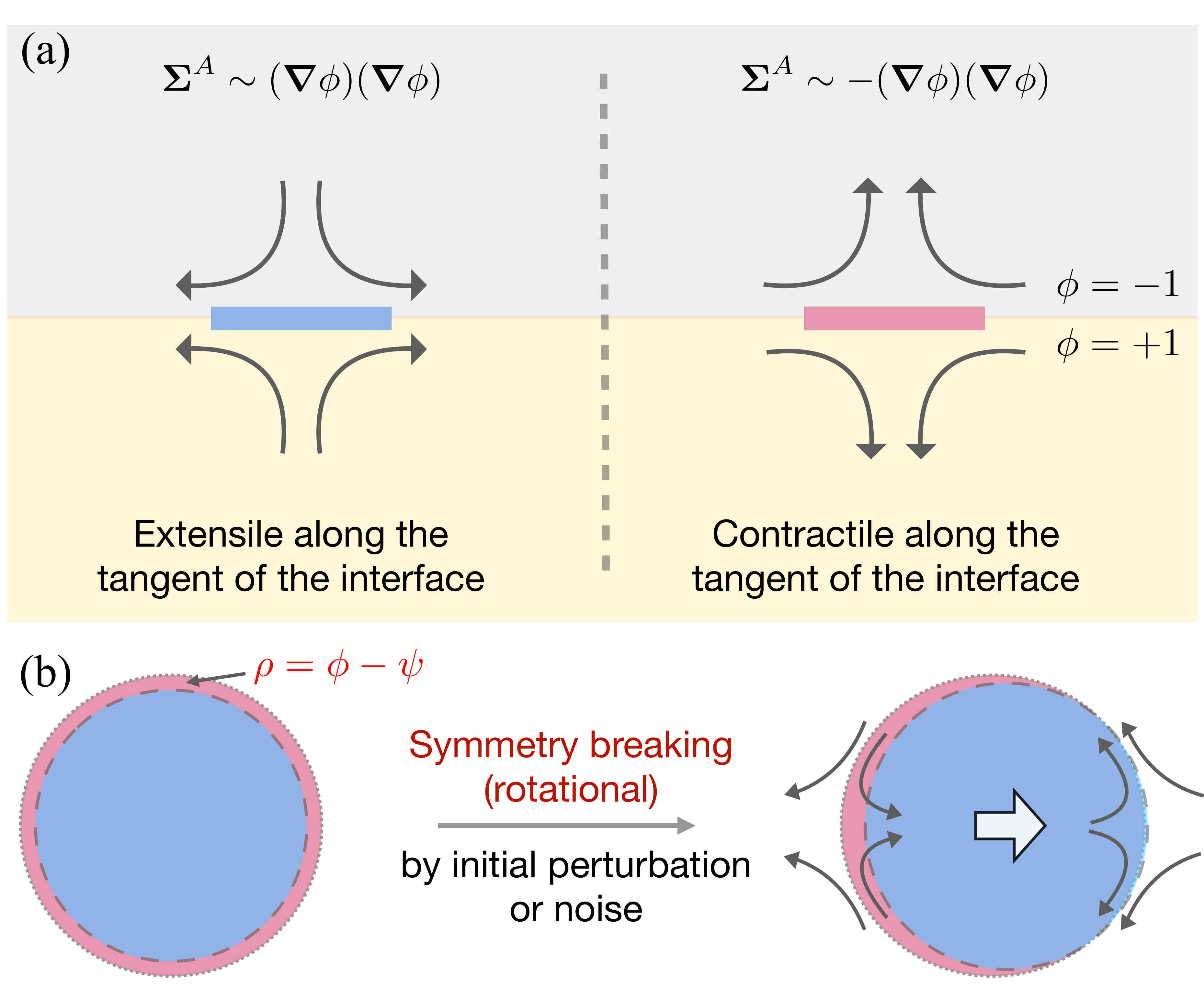
Figure 1: (a) Flow driven by an active stress $\boldsymbol{\Sigma}^{A}$ on the interface of the droplet phase field $\phi$. A positive (negative) $\boldsymbol{\Sigma}^{A}$ implies an extensile (contractile) - shown by a blue (red) patch - fluid flow tangential to the $\phi$-interface. (b) A cell is represented by $\phi$-droplet, while the concentration of actomyosin in the cell cortex is given by $\phi\mathcal{-}\psi$ (red ring). Under a small random initial perturbation, the $\psi>0$ domain is displaced to the front (right), creating excess contractile stress at the back. This leads to an active flow which locks the $\psi$-droplet in the front, causing sustained self-propulsion along a direction selected by spontaneous symmetry breaking.

In this Rapid Communication, we present a field theory of self-propelling active droplets, such as cells, in the absence of liquid-crystalline order. Our theory is given in terms of two scalar fields $\phi$ and $\psi$, which follow symmetry arguments of the Landau theory Chaikin and Lubensky (2000), coupled by the active stress in the momentum conservation equation. The $\phi$-field delineates the interior/exterior of the droplet. The $\psi$ field is an auxilary field which is related to a conserved scalar describing the local amount of active material ($\rho$). It is defined via $\rho=\phi-\psi$. The arrangement of interest is where a cortex of nonzero $\rho$ [see the red region in Fig.1(b)] resides in the outer part of an otherwise passive droplet with constant overall mass density. This arrangement corresponds to a droplet with $\psi>0$ [see the blue core in Fig.1(b)] superimposed on a larger droplet of $\phi>0$. The difference of the two radii is then the thickness of a cortex surrounding the droplet, rendered contractile by, e.g., the action of myosin motors.

Self-propulsion of the active droplet emerges generically by the spontaneous breakdown of rotational symmetry in the $\rho$ field. Once this is broken, the droplet moves with a speed that increases linearly with the activity strength and decreases linearly with the droplet area fraction within a periodic domain. (We rationalize both scalings analytically.) We then extend our theory to study an array of active droplets and identify an active-Crowley-like instability.

Model: First, with two conserved scalar fields $\phi(\boldsymbol{r},t)$ and $\psi(\boldsymbol{r},t)$, we choose the free energy functional $\mathcal{F}[\phi,\psi]$ as:

$$\mathcal{F}[\phi,\psi] =\int\Big{(}\frac{a}{2}\phi^{2}+\frac{b}{4}\phi^{4}+\frac{a^{\prime}}{2}\psi^{2}+\frac{b^{\prime}}{4}\psi^{4}-\beta\phi\psi$$

$$+\frac{\kappa}{2}|\boldsymbol{\nabla}\phi|^{2}+\frac{\kappa^{\prime}}{2}|\boldsymbol{\nabla}\psi|^{2}\Big{)}\,d\boldsymbol{r},$$ (1)

where $a=-b<0$, $a^{\prime}=-b^{\prime}<0$ and $\kappa,\kappa^{\prime},\beta>0$. Although we choose $a=a^{\prime}$ and $b=b^{\prime}$, our results are robust against changing these parameters as long as the free energy admits the solution for a stable droplet. Connections of these free energy parameters to physical parameters - surface tension, interfacial width, thickness of cortex, etc - are given in Table 1 of the SI.

Eq. (1) is adopted as the simplest way to stabilize two concentric phase-field domains (in $\phi$ and $\psi$) of unequal size. On identification of $\rho=\phi-\psi$, this becomes a droplet surrounded by a cortex, as required. Parameters are chosen so that each phase field approaches $\pm 1$ in the interior/exterior bulk phases. The $\beta>0$ term is an energetic coupling which favors maximizing the overlap of $\psi$ and $\phi$ fields. Since both fields are conserved, the volumes of these $\phi,\psi$ droplets (equivalently, the $\phi$ droplet and its $\phi-\psi$ cortex) are separately constant in time. We choose the initial volume of the $\phi$-droplet to be bigger than of the $\psi$-droplet, and thus, the $\psi$-droplet resides within the $\phi$-droplet giving a cortex in between [see Fig. 1(b)]. The $\phi$-droplet then has interfacial tension $\gamma_{0}\simeq\sqrt{-8\kappa a^{3}/9b^{2}}$ Cates and Tjhung (2017), with similar expressions for the $\psi$-droplet. These tensions govern respectively the cortex/exterior and cortex/interior interfaces. Note that the $\beta$-term also renormalizes the interfacial tension $\gamma_{0}$; however, we choose $\beta/a=\beta/a^{\prime}=0.01$, so that this difference is not appreciable.

The only active term in our model is a contractile stress, which lives, for simplicity, at the outer interface where $\phi$ passes through zero. This active stress is, however, modulated by the local concentration of cortical material which (in some units) is $\rho(\boldsymbol{r},t)=\phi-\psi\simeq-\psi>0$ [see Fig. 2(a)]. If rotational symmetry is maintained, the cortex is concentric with the droplet and the active stress is likewise symmetric (Fig. 1(b), left). In the broken symmetry state, with more cortical material at the rear of the droplet, the active stress is larger there, creating a fluid flow that sustains the broken symmetry, by sweeping the cortex of actomyosin towards the rear so that $-\psi$ is larger there than at the front [Fig. 1(b) right].

This flow is governed by the hydrodynamic velocity $\boldsymbol{v}(\boldsymbol{r},t)$, which describes the average velocity of the cellular materials plus the solvent. The conserved dynamics of $\phi$ and $\psi$ is then as follows:

$$\frac{\partial\phi}{\partial t}+\boldsymbol{\nabla}\cdot\left(\phi\boldsymbol{v}-M^{\phi}\boldsymbol{\nabla}\frac{\delta\mathcal{F}}{\delta\phi}\right) =0,$$ (2a)

$$\frac{\partial\psi}{\partial t}+\boldsymbol{\nabla}\cdot\left(\psi\boldsymbol{v}-M^{\psi}\boldsymbol{\nabla}\frac{\delta\mathcal{F}}{\delta\psi}\right) =0,$$ (2b)

such that the total $\int\phi\,d\boldsymbol{r}$ and $\int\psi\,d\boldsymbol{r}$ are constant in time. The first term inside the parentheses describes advection of $\phi$ and $\psi$ by the fluid velocity $\boldsymbol{v}$. The second term describes diffusion of $\phi$ and $\psi$ along the negative gradient of the chemical potential $\delta\mathcal{F}/\delta\phi$ and $\delta\mathcal{F}/\delta\psi$, respectively. $M^{\phi,\psi}>0$ are the mobilities for each field.

In the limit of low Reynolds number, which is appropriate for sub-cellular materials, the fluid flow $\boldsymbol{v}(\boldsymbol{r},t)$ is obtained from solving the Stokes equation:

$$\boldsymbol{\nabla}\cdot(\boldsymbol{\sigma}+\boldsymbol{\Sigma}^{E}+\boldsymbol{\Sigma}^{A})=\mathbf{0},$$ (3)

where $\boldsymbol{\sigma}=-p\boldsymbol{I}+\eta[(\boldsymbol{\nabla}\boldsymbol{v})+(\boldsymbol{\nabla}\boldsymbol{v})^{T}]$ is the Cauchy stress tensor in a fluid of viscosity $\eta$, $\boldsymbol{I}$ is the identity matrix, and $p$ is the isotropic pressure, which enforces the incompressibility condition $\boldsymbol{\nabla}\cdot\boldsymbol{v}=0$. $\boldsymbol{\Sigma}^{E}$ in (3) is the equilibrium interfacial stress, which is derived from the free energy functional (1) Cates and Tjhung (2017):

$$\boldsymbol{\Sigma}^{E}=-\kappa(\boldsymbol{\nabla}\phi)(\boldsymbol{\nabla}\phi)-\kappa^{\prime}(\boldsymbol{\nabla}\psi)(\boldsymbol{\nabla}\psi).$$ (4)

Physically, $\boldsymbol{\Sigma}^{E}$ is the elastic response to a deformation in the interface of the $\phi$- and $\psi$-droplet.

$\boldsymbol{\Sigma}^{A}$ in (3) is the active stress, which drives the system out of equilibrium. The form of $\boldsymbol{\Sigma}^{A}$ is adapted from the active model H Tiribocchi et al. (2015); Singh and Cates (2019):

$$\boldsymbol{\Sigma}^{A}=\alpha\psi(\boldsymbol{\nabla}\phi)(\boldsymbol{\nabla}\phi),$$ (5)

where $\alpha\geq 0$ is a cortical contractile activity parameter, such that the equilibrium limit is recovered when $\alpha\rightarrow 0$. From (5), the activity is always localized at the interface of the $\phi$-droplet. This differs from other models of active fluid droplets such as active nematics Tjhung et al. (2012); Blow et al. (2014); Guillamat et al. (2018); Giomi and DeSimone (2014), where the active stress affects the bulk of the interior. The physical significance of $\boldsymbol{\Sigma}^{A}$ is illustrated in Fig. 1(a). Consider a patch of active region on an interface separating $\phi=+1$ and $\phi=-1$ regions (see Fig.1a). If $\alpha\psi>0$ so that $\boldsymbol{\Sigma}^{A}\propto(\nabla\phi)(\nabla\phi)$, the active stress creates an extensile fluid flow in the tangential direction of the interface. On the other hand if $\alpha\psi<0$, as will hold here, $\boldsymbol{\Sigma}^{A}\propto-(\nabla\phi)(\nabla\phi)$, and the active stress creates a contractile flow tangential to the interface, corresponding to actomyosin contractility $\alpha>0$ in the cell cortex. (Recall that the density of this cortex is $\rho\sim-\psi>0$ at the outer droplet interface.) Note that in the literature on active phase separation Tiribocchi et al. (2015); Singh and Cates (2019), contractile and extensile are defined with respect to the microswimmer orientation, normal to the interface. The opposite convention, chosen here, refers to the tangential cortex layer and is used in the cellular literature Hawkins et al. (2011); Poincloux et al. (2011).

Our numerical system consists of a two-dimensional (2D) square box with linear size $L$ and periodic boundary conditions. We initialize a $\phi$-droplet with radius $R$ at the centre of the box, and similarly a $\psi$-droplet with a smaller radius $0.9R$; see Fig. 1(b) left. We then solve Eqns. (2a-3) numerically using a pseudo-spectral method, as detailed in the SI App .

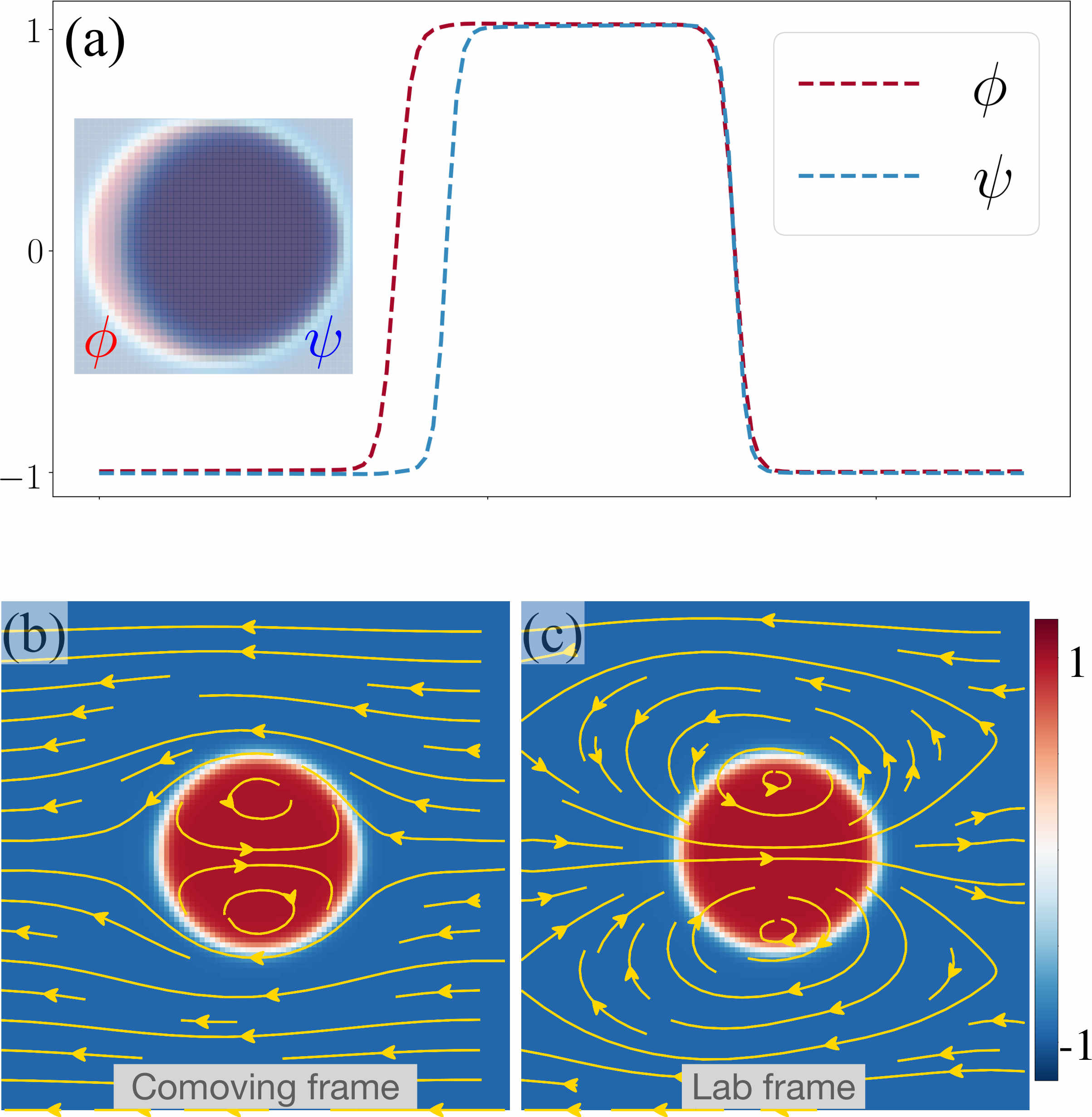
Figure 2: (a) Inset: A snapshot of an active droplet steadily moving in the $x$-direction. Main: Corresponding plots of $\phi$ and $\psi$ as a function of $x$ at the cross-section passing through the centre of the droplet. (b) and (c) show the streamlines of the fluid flow of the same active droplet in (b) the comoving frame and (c) laboratory frame. The streamlines are superimposed on the pseudo-color plot of the $\phi$-field.

Mechanism of self-propulsion: Now we will illustrate the mechanism for self-propulsion. We fix the activity $\alpha$ to be finite and positive. First, let us consider what happens when both $\phi$- and $\psi$-droplets are concentric as shown in Fig. 1(b) left. At the interface of the $\phi$-droplet, the value of $\psi$ is negative and the same everywhere along the interface ($\psi\simeq-1$). Thus, the active stress $\boldsymbol{\Sigma}^{A}$ (5) is contractile and its magnitude is the same everywhere along the interface. This represents an isotropic distribution of active cortex material, and thus, by symmetry, we should not expect to see any motion.

Now imagine that we give a small displacement (which can come either from thermal fluctuations or an initial perturbation – we consider the latter case here) to the $\psi$-droplet as shown in Fig. 1(b) right. The essence of the symmetry breaking mechanism can be understood by considering a small initial displacement of the smaller droplet $\psi$ such that the interface of the $\phi$ droplet touches that of the $\psi$ droplet at one point (found below to be the ‘front’ of the droplet when in motion) so that the $\rho$ cortex vanishes in thickness at this point. Therefore at the front, the active stress $\boldsymbol{\Sigma}^{A}$ (5) is approximately zero, whereas at the back, the active stress is finite and contractile. This excess contractile stress at the back pulls the fluid from the front to the back along the interface of $\phi$, as indicated by black arrows in Fig. 1(b) right. This translates into persistent motion. Fig. 2(a) shows the values of $\phi$ and $\psi$ measured at the cross-section, which supports this mechanism. Physically, we have an accumulation of actomyosin at the back of the cell which creates excess contractility at the rear cell cortex. This is consistent with experiments on cellular swimming motility in the absence of any boundary on which to crawl Poincloux et al. (2011); Ruprecht et al. (2015).

Fig. 2(b,c) show the steady state fluid velocity from the full hydrodynamic simulations in the co-moving (b) and laboratory frame (c). This fluid flow is as schematically shown in Fig. 1(b) right. Inside the $\phi$-droplet, the differential active stress at the interface generates a pair of counter-rotating vortices, which then squash the $\psi$-droplet further to the front, giving a positive feedback.

Incidentally, this type of fluid flow is generic to all neutral (pure quadrupolar flow Kim and Karrila (1991)) squirmer droplets, whose motion is typically driven by Marangoni flow along the interface Thutupalli et al. (2011); Jin et al. (2017); Izzet et al. (2019). From Figs. 1(b) and 2(a), in the front hemisphere, $\psi=\psi_{f}\simeq 0$, whereas in the back hemisphere, $\psi=\psi_{b}\simeq-1$. The active stress $\boldsymbol{\Sigma}^{A}$ renormalizes the surface tension into an effective surface tension, $\gamma_{0}\rightarrow\gamma=\gamma_{0}(1-\alpha\psi/\kappa)$ Tiribocchi et al. (2015); Singh and Cates (2019), where $\gamma_{0}=\sqrt{-8\kappa a^{3}/9b^{2}}$ Cates and Tjhung (2017) is the surface tension without activity, $\alpha=0$. This has the effect of a net change in surface tension between the front and rear of the $\phi$-droplet, which is $\Delta\gamma=\alpha\Delta\psi\gamma_{0}/\kappa$, where $\Delta\psi=\psi_{f}-\psi_{b}$. Thus, we have a Marangoni flow from low effective surface tension (front) to high effective surface tension (back) as shown in Fig. 2(b), while Fig. 2(c) contains the same flow in the laboratory frame. The corresponding theoretical flow around an active droplet, in an infinite 2D domain, is given in the first figure of App .

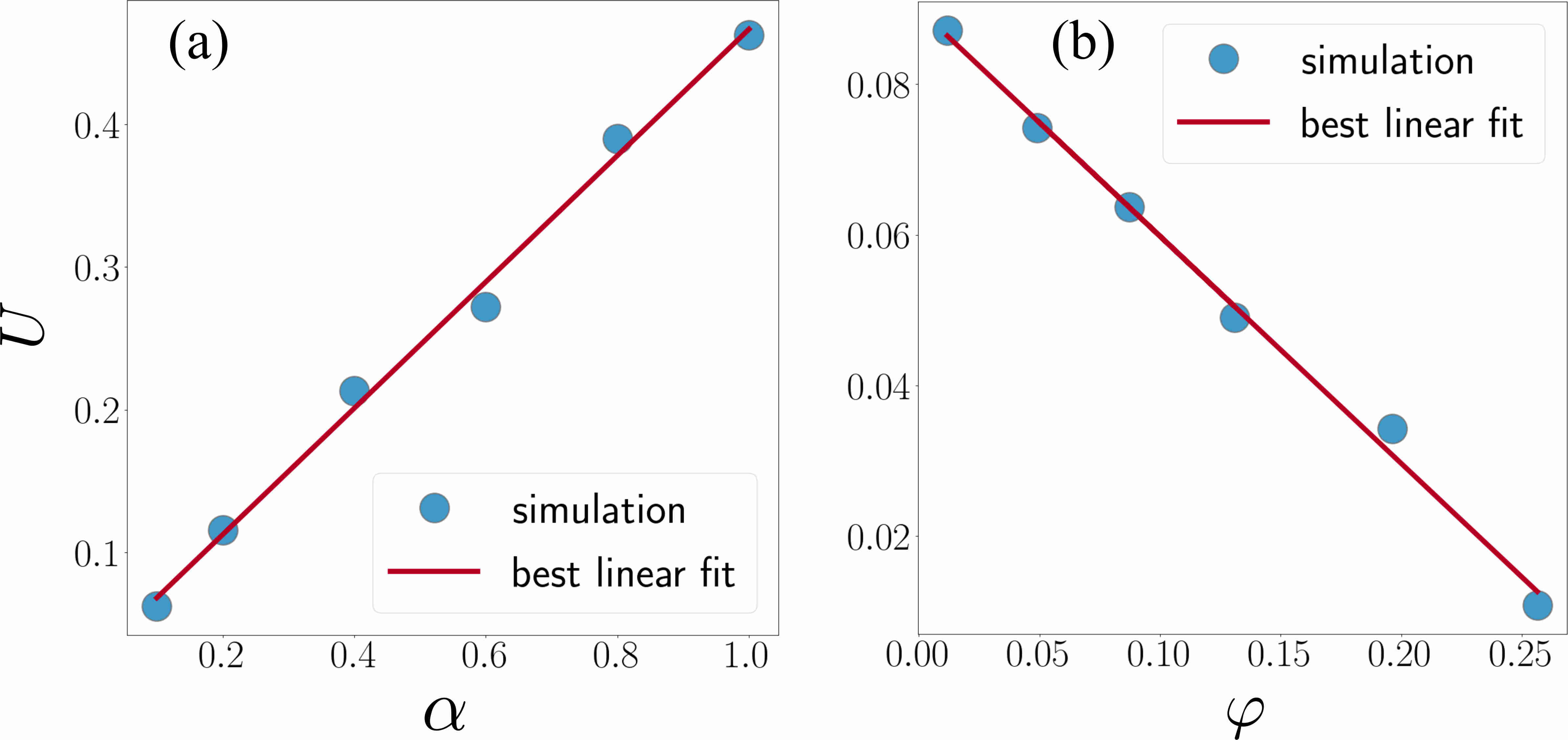
Figure 3: (a) The self-propulsion speed of the droplet $U$ increases linearly with the activity parameter $\alpha$ at a fixed area fraction $\varphi=\pi R^{2}/L^{2}=0.049$. (b) The self-propulsion speed of the droplet $U$ decreases linearly with the area fraction $\varphi$ for a fixed $\alpha=0.2$. From the best linear fit of the simulation data we obtain $U=0.44\alpha\left(1-3.4\varphi\right)$, while the theoretical estimate of Eq.(7) is $U=0.49\alpha$ in the limit $\varphi\rightarrow 0$.

Self-propulsion speed, $U$: Having described the mechanism, we now obtain an analytical expression for $U$ using appropriate boundary conditions corresponding to our model. In simulations, the interface is diffused, and thus, there is no discontinuity in the fluid velocities inside ($\tilde{\boldsymbol{v}}$) and outside (${\boldsymbol{v}}$) the droplet. In analytical calculations, the interface is sharp, and we solve the Stokes equation both inside and outside of the droplet using the following boundary conditions

$$v_{r}(r=R) =\tilde{v}_{r}(r=R)=0,$$ (6a)

$$v_{\theta}(r=R) =\tilde{v}_{\theta}(r=R),$$ (6b)

$$\left(\boldsymbol{\sigma}-\tilde{\boldsymbol{\sigma}}\right)\cdot\hat{\boldsymbol{r}} =\gamma\left(\boldsymbol{\nabla}\cdot\hat{\boldsymbol{r}}\right)\hat{\boldsymbol{r}}-\boldsymbol{\nabla}\gamma,\quad\text{at }r=R.$$ (6c)

The above equations represent no-flux (6a), continuity of tangential slip velocity (6b) at the interface, and the fact that the discontinuity of the Cauchy stress, $\boldsymbol{\sigma}$, at the interface is related to the surface tension $\gamma(\theta)$ of the droplet, via (6c) Schmitt and Stark (2016); Leven and Newman (1976). The speed $U_{0}$ of the droplet in an infinite 2D domain (see App ) is then:

$$U_{0}=\frac{\Delta\gamma}{16\eta},$$ (7)

As described previously $\Delta\gamma=\alpha\Delta\psi\gamma_{0}/\kappa$, and thus, the speed increases linearly with contractile activity $\alpha$ and actomyosin concentration in the cortex $\rho$. Using the above formula and the parameters of Fig. 3, the theoretically predicted speed is $U_{0}=0.49\alpha$. This is in excellent agreement with the numerical estimate of $U_{0}=0.44\alpha$ obtained from a best-fit of the simulation data of Fig. 3. It should be noted that the speed does not depend on $R$, which is consistent with the literature on transport by interfacial forces Anderson (1989); Schmitt and Stark (2016). We ignore any deformations of the droplet in our calculations. A more detailed analysis studying the role of deformation will be pursued in a future work.

To account for the periodic boundary conditions used in simulations, we need to sum the flow due to periodic images of the droplet, which lie on a 2D square lattice. The expression for the speed $U$ is then $U=U_{0}(1-\varphi)$ (App, ). The best fit of numerical data in Fig. 3 gives $U=0.44\alpha\left(1-3.4\varphi\right)$. Although our analytical results give the linear scalings for the self-propulsion speed, as a function of activity parameter $\alpha$ and area fraction $\varphi$, seen in the simulations, this belies the true complexity of the problem which exhibits linear scaling with volume fraction far beyond any perturbative regime (and indeed with a different coefficient). A more detailed analysis of the above will be pursed in a future work.

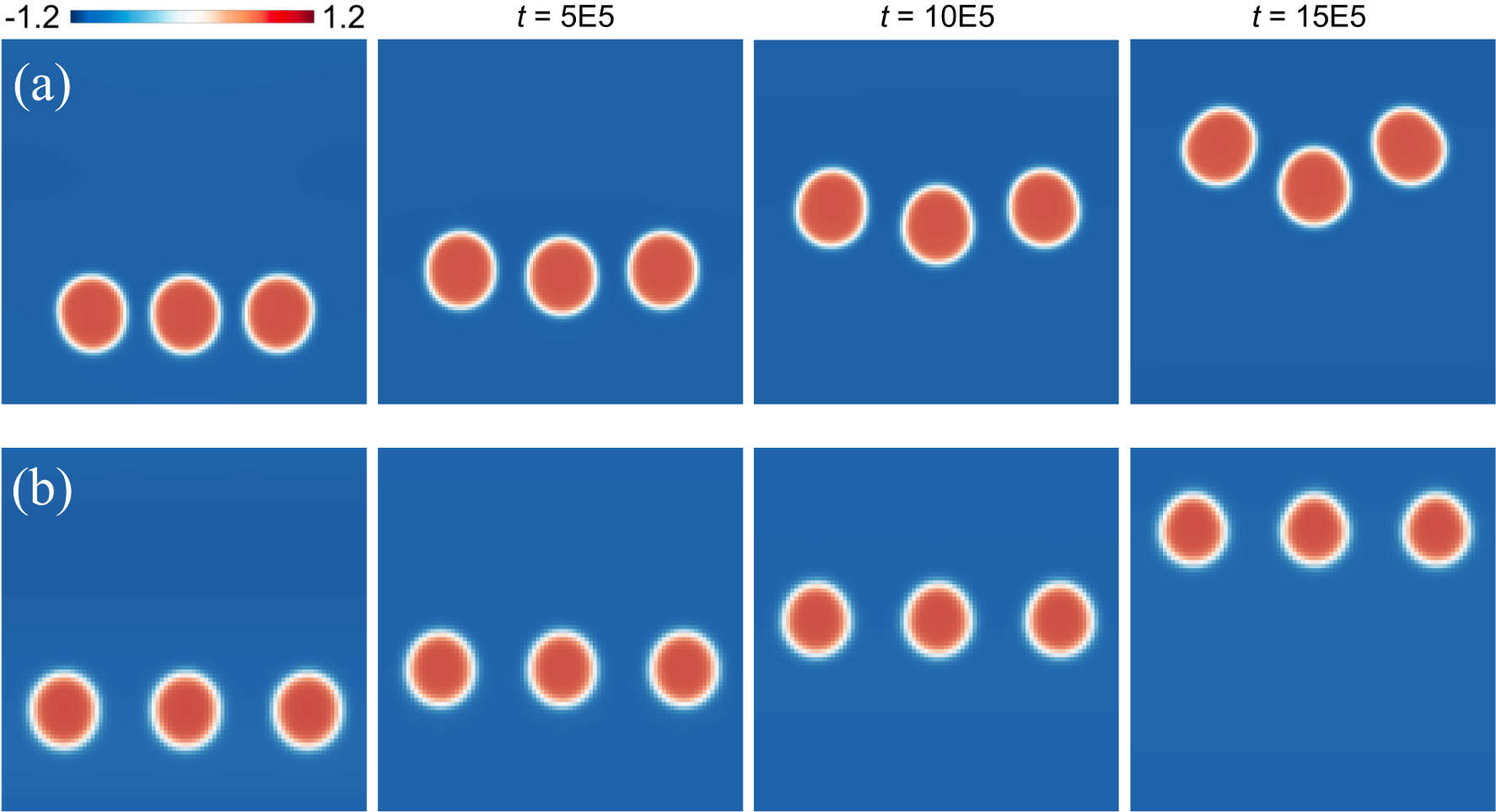
Figure 4: (a) Active-Crowley-like instability: A linear array of active droplets is unstable. This instability is opposite to that in an array of sedimenting particles. (b) There is no instability if there is no well-defined central particle.

Crowley-like instability of an array of active droplets: The model and simulations above can be easily extended to the case of multiple droplets. This is operationally done by generalizing the free energy functional of (1) for $N$ active droplets as:

$$\mathcal{F}[\boldsymbol{\phi},\boldsymbol{\psi}] =\int\sum_{i=1}^{N}\Big{(}\frac{a}{2}\phi_{i}^{2}+\frac{b}{4}\phi_{i}^{4}+\frac{a^{\prime}}{2}\psi_{i}^{2}+\frac{b^{\prime}}{4}\psi_{i}^{4}-\beta\phi_{i}\psi_{i}$$

$$+\frac{\kappa}{2}(\boldsymbol{\nabla}\phi_{i})^{2}+\frac{\kappa^{\prime}}{2}(\boldsymbol{\nabla}\psi_{i})^{2}+\sum_{j\neq i}\beta^{\prime}\phi_{i}\phi_{j}\Big{)}d\boldsymbol{r}.$$ (8)

Here the term proportional to $\beta^{\prime}>0$ effectively leads to repulsion between the droplet $\phi_{i}$ and $\phi_{j}$ Foglino et al. (2017), and thus, precludes any overlap. The dynamics for each $\phi_{i}$, $\psi_{i}$ and $\boldsymbol{v}$ is the same as in (2a-3) and the equilibrium interfacial stress $\boldsymbol{\Sigma}^{E}$ and active stress $\boldsymbol{\Sigma}^{A}$ are now the sum of each contribution from $\phi_{i}$ and $\psi_{i}$ given in (4) and (5).

We use the above to study the instability in a linear array of three droplets as shown in Fig. 4. We see an active-Crowley-like instability when there is a well-defined central particle. Unlike in the case of the sedimentation Ramaswamy (2001), here the central particle lags. This can be understood from the fluid flow in Fig. 2(c), which has the effect of the central particle being pushed backwards by the neighboring particles. On the other hand if the particles are equally separated as in Fig. 4(b), there is no instability as there is no well-defined central particle, when taking into account the periodic boundary condition used.

Conclusion: We have presented a minimal (and scalable) hydrodynamic model of active droplets without any liquid-crystalline order parameter Tjhung et al. (2012, 2015). Nor do we require explicit chemical reactions in the form of source and sink terms Yabunaka et al. (2012); Fadda et al. (2017); Morozov and Michelin (2019a); Lavi et al. (2020). The self-propulsion of droplets in our model relies on the fact that excess contractility in the back of the droplet gives rise to a finite effective surface tension gradient, $\Delta\gamma\neq 0$. Thus, although motivated by a simple description of swimming cells, our model can also capture the self-propulsion due to Marangoni stresses on the surface of active emulsion droplets Thutupalli et al. (2011); Jin et al. (2017); Thutupalli et al. (2018); Izzet et al. (2019); Morozov and Michelin (2019b); Lohse and Zhang (2020). The effective tension in our case is not a prescribed quantity, but is instead, a consequence of the minimal form of the active stress $\boldsymbol{\Sigma}^{A}$ given in Eq.(5). Our theory might possibly be extended to address a passive liquid crystal inside an active scalar droplet, to mimic experimental systems of Thutupalli et al. (2018, 2011), or, in the chiral case, the helical trajectories seen in experiments of Yamamoto and Sano (2017).

We also showed the feasibility of our model for the study of many droplets by studying an active Crowley-like instability in a linear array of active droplets. A more detailed study of an active droplet suspension using our theory and its comparison to the particulate theories Shaebani et al. (2020) of active matter will be presented in future work.

RS is funded by a Royal Society-SERB Newton International Fellowship. MEC is funded by the Royal Society. Numerical work was performed on the Fawcett HPC system at the Centre for Mathematical Sciences. Work funded in part by the European Research Council under the Horizon 2020 Programme, ERC grant agreement number 740269.

Supplemental Information (SI)

I Stokes flow of a self-propelling droplet in infinite two-dimensions

In this Section, we will derive the analytic solution for the fluid velocity in the limit of infinite boundary ($L\rightarrow\infty$) and sharp $\phi$-interface ($\xi_{0}\rightarrow 0$). We consider a two-dimensional active droplet swimming with velocity $-U_{0}\hat{\boldsymbol{x}}$ in the lab frame. In the co-moving frame, the droplet will be stationary, and the fluid velocity at far field $r\rightarrow\infty$ is $U_{0}\hat{\boldsymbol{x}}$. We can then define $\boldsymbol{v}(\boldsymbol{r})$ and $\tilde{\boldsymbol{v}}(\boldsymbol{r})$ to be the fluid velocity inside and outside the droplet respectively; $\boldsymbol{v}(\boldsymbol{r})$ and $\tilde{\boldsymbol{v}}(\boldsymbol{r})$ are obtained from solving two independent Stokes equation. We then match the two solutions at the interface of the droplet $r=R$ via the boundary conditions in Eq.(6) of the main text. We can assume the droplet to be centered at the origin. It is convenient to obtain the solution of the fluid flow using stream-function $\vartheta$, defined as $\boldsymbol{v}=\boldsymbol{\nabla}\times(\vartheta\hat{\boldsymbol{z}})$ Happel and Brenner (1981). The components of the fluid velocity are given in terms of the stream-function in Cartesian $(x,y)$ and plane polar $(r,\theta)$ coordinates as

$$v_{x}=\frac{\partial\vartheta}{\partial y},\quad v_{y}=-\frac{\partial\vartheta}{\partial x},\quad v_{r}=\frac{1}{r}\frac{\partial\vartheta}{\partial\theta},\quad v_{\theta}=-\frac{\partial\vartheta}{\partial r}.$$ (9)

Now using the incompressibility condition $\boldsymbol{\nabla}\cdot\boldsymbol{v}=0$ and Stokes equation, it can be shown by standard arguments that the stream-function satisfies the biharmonic equation:

$$\nabla^{4}\vartheta=0,$$ (10)

subject to the boundary conditions for the corresponding velocity field given in the main text.

Now let us denote $\boldsymbol{v}=\boldsymbol{\nabla}\times(\vartheta\hat{\boldsymbol{z}})$ and $\tilde{\boldsymbol{v}}=\boldsymbol{\nabla}\times(\tilde{\vartheta}\hat{\boldsymbol{z}})$ to be the fluid velocity inside and outside the droplet respectively.

Exterior flow $\boldsymbol{v}$: First, we will solve the fluid velocity outside the droplet. The boundary condition for the fluid velocity at infinity $r\rightarrow\infty$ is:

$$v_{x}=\frac{\partial\vartheta}{\partial y}=U_{0},\quad\text{as }r\rightarrow\infty.$$ (11)

This implies that the stream-function has the following form at $r\rightarrow\infty$:

$$\vartheta(r,\theta)=U_{0}r\sin\theta,\quad\text{as }r\rightarrow\infty.$$ (12)

Thus we can use separation of variables:

$$\vartheta(r,\theta)=f(r)\sin\theta.$$ (13)

Substituting (13) into (10), $f(r)$ satisfies the following equation:

$$\left(\frac{d^{2}}{dr^{2}}+\frac{1}{r}\frac{d}{dr}-\frac{1}{r^{2}}\right)^{2}f(r)=0.$$ (14)

Using trial solution $f(r)\sim r^{n}$, we can obtain the general solution to (14):

$$f(r)=\frac{A}{r}+Br+Cr\ln r+Dr^{3}.$$ (15)

From the boundary condition (12), we get $C=D=0$ and $B=U_{0}$.

Now the no-flux boundary condition for the normal component of the velocity at the interface $r=R$ reads:

$$v_{r}(R,\theta)=\frac{1}{R}\left.\frac{\partial\vartheta}{\partial r}\right|_{r=R}=0.$$ (16)

This implies $A=-U_{0}R^{2}$. Thus the exterior fluid velocity in polar coordinates and co-moving frame is:

$$v_{r}(r,\theta) =U_{0}\left(-\frac{R^{2}}{r^{2}}+1\right)\cos\theta$$ (17)

$$v_{\theta}(r,\theta) =-U_{0}\left(\frac{R^{2}}{r^{2}}+1\right)\sin\theta.$$ (18)

Interior flow $\tilde{\boldsymbol{v}}$: Again, defining the stream-function $\tilde{\vartheta}(r,\theta)$ and using separation of variables, the solution to the biharmonic equation (10) is

$$\tilde{\vartheta}(r,\theta)=\left(\frac{\tilde{A}}{r}+\tilde{B}r+\tilde{C}r\ln r+\tilde{D}r^{3}\right)\sin\theta.$$ (19)

Now since the fluid velocity $\tilde{\boldsymbol{v}}=\boldsymbol{\nabla}\times(\tilde{\vartheta}\hat{\boldsymbol{z}})$ has to remain finite at $r=0$, we then require $\tilde{A}=\tilde{C}=0$. We then impose no-flux boundary condition:

$$\tilde{v}_{r}(R,\theta)=\frac{1}{R}\left.\frac{\partial\vartheta}{\partial\theta}\right|_{r=R}=0,$$ (20)

and continuity of the tangential velocity at the interface:

$$\tilde{v}_{\theta}(R,\theta)=v_{\theta}(R,\theta),$$ (21)

to finally find: $\tilde{B}=-U_{0}$ and $\tilde{D}=U_{0}/R^{2}$. Thus the interior fluid velocity in polar coordinates is:

$$\tilde{v}_{r}(r,\theta) =U_{0}\left(-1+\frac{r^{2}}{R^{2}}\right)\cos\theta$$ (22)

$$\tilde{v}_{\theta}(r,\theta) =U_{0}\left(1-\frac{3r^{2}}{R^{2}}\right)\sin\theta$$ (23)

This fluid flow, derived from above expressions for the interior and exterior region, has been plotted in Fig.(5). This can be compared with direct numerical simulations in the main text. It is worthwhile to note that there is no solution for Stokes flow around a disc, the so-called Stokes paradox Happel and Brenner (1981), if a no-slip boundary condition at $r=R$ is used. The solution described above relies on the fact that there is a free-slip boundary condition on the surface of the droplet.

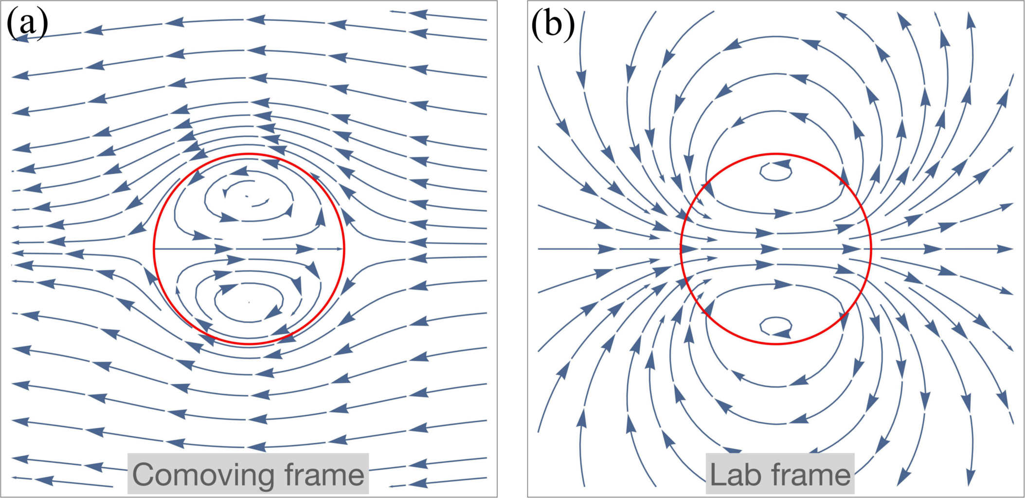
Figure 5: Streamlines of the theoretical fluid flow around an active droplet moving to the right in the co-moving (a) and lab-frame (b) in an infinite domain. The red circle denotes the interface of the droplet. (Note that the calculation in Section I is done with the droplet moving to the left, thus the fluid velocity above is flipped around the $y$-axis.)

Self-propulsion speed: The hydrodynamic stress is discontinuous at the interface $r=R$ due to the surface tension $\gamma(\theta)$:

$$\left(\boldsymbol{\sigma}-\tilde{\boldsymbol{\sigma}}\right)\cdot\hat{\boldsymbol{r}}=\gamma\left(\boldsymbol{\nabla}\cdot\hat{\boldsymbol{r}}\right)\hat{\boldsymbol{r}}-\boldsymbol{\nabla}\gamma,\quad\text{at }r=R.$$ (24)

The stress in polar coordinates is:

$$\sigma_{rr} =-p+2\eta\frac{\partial v_{r}}{\partial r}$$ (25)

$$\sigma_{\theta\theta} =-p+2\eta\left(\frac{1}{r}\frac{\partial v_{\theta}}{\partial\theta}+\frac{v_{r}}{r}\right)$$ (26)

$$\sigma_{\theta r} =\sigma_{r\theta}=\eta\left(\frac{1}{r}\frac{\partial v_{r}}{\partial\theta}+\frac{\partial v_{\theta}}{\partial r}-\frac{v_{\theta}}{r}\right).$$ (27)

First, let us look at the $r$-component of (24):

$$\sigma_{rr}-\tilde{\sigma}_{rr}=\frac{\gamma}{R}\quad\Longrightarrow\quad\tilde{p}-p=\frac{\gamma}{R},$$ (28)

which is just the Laplace pressure difference between the interior and exterior of the droplet. Now we look at the $\theta$-component of (24):

$$\sigma_{\theta r}-\tilde{\sigma}_{\theta r} =-\frac{1}{R}\frac{d\gamma}{d\theta}$$ (29)

$$\eta\frac{\partial v_{\theta}}{\partial r}-\tilde{\eta}\frac{\partial\tilde{v}_{\theta}}{\partial r} =-\frac{1}{R}\frac{d\gamma}{d\theta},\quad\text{at }r=R$$ (30)

where $\eta$ and $\tilde{\eta}$ is the fluid viscosity inside and outside the droplet respectively. Now substituting (18) and (23) into (30), we get:

$$U_{0}\sin\theta=-\frac{1}{8\eta}\frac{d\gamma}{d\theta}.$$ (31)

Thus, the velocity of the droplet is non-zero only if we have a surface tension gradient along the tangential direction. Now we can average (31) over the angle $\theta\in[0,\pi]$ to obtain:

$$U_{0}=\frac{\Delta\gamma}{16\eta},$$ (32)

where $\Delta\gamma$ is the surface tension difference between the back and the front. Note that $\theta=\pi$ corresponds to the front the droplet and $\theta=0$ corresponds to the back of the droplet. For active model H Tiribocchi et al. (2015), the effective surface tension is $\gamma=\gamma_{0}(1-\alpha\psi/\kappa)$, and thus we get:

$$U_{0}=\frac{\gamma_{0}\alpha}{16\eta\kappa},$$ (33)

since $\psi=0$ in the front and $\psi=-1$ in the back (see Fig. 1 in the main text). Thus, we obtain linear scaling with activity $\alpha$, consistent with the numerical result in the main text.

II Active droplets on a lattice

To compute this finite size scaling theoretically, we consider an infinite array of active droplets, whose centre of mass are located on a square lattice. The renormalized fluid velocity in the region around the central droplet, located at the origin, is the sum of all the fluid velocities generated by each droplet on the lattice. The numerical simulations presented in the main text assume periodic boundary condition on each side of the box: $(x,\pm L/2),(\pm L/2,y)$. This is equivalent to having an infinite number of active droplets located on a square lattice $(mL,nL)$, where $m,n\in\mathbb{Z}$. In this Section, we will derive the approximate fluid velocity generated by these droplets.

First, let us consider the dilute limit $R/L\rightarrow 0$ (Section I). Let us consider an active droplet swimming with velocity $U_{0}\hat{\boldsymbol{x}}$ and located at the origin. The fluid flow generated by this single droplet in the lab frame is (see Fig. 5(b) and Eqns. (17-18)):

$$u_{x} =U_{0}R^{2}\frac{x^{2}-y^{2}}{(x^{2}+y^{2})^{2}}$$ (34)

$$u_{y} =2U_{0}R^{2}\frac{xy}{(x^{2}+y^{2})^{2}}.$$ (35)

In particular, the fluid flow at the leading edge of a single droplet $(x,y)=(R,0)$ is equal to the velocity of the droplet itself:

$$u_{x}(R,0)=U_{0}.$$ (36)

Now, the fluid flow generated by infinite droplets in a lattice is given by (assuming dilute flow solution for each droplet):

$$u_{x}= U_{0}R^{2}\frac{x^{2}-y^{2}}{(x^{2}+y^{2})^{2}}$$

$$+U_{0}R^{2}\sum_{m=1}^{\infty}\sum_{n=0}^{\infty}\frac{(x-mL)^{2}-(y-nL)^{2}}{\left[(x-mL)^{2}+(y-nL)^{2}\right]^{2}}$$

$$+U_{0}R^{2}\sum_{m=0}^{-\infty}\sum_{n=1}^{\infty}\frac{(x-mL)^{2}-(y-nL)^{2}}{\left[(x-mL)^{2}+(y-nL)^{2}\right]^{2}}$$

$$+U_{0}R^{2}\sum_{m=0}^{\infty}\sum_{n=-1}^{-\infty}\frac{(x-mL)^{2}-(y-nL)^{2}}{\left[(x-mL)^{2}+(y-nL)^{2}\right]^{2}}$$

$$+U_{0}R^{2}\sum_{m=-1}^{-\infty}\sum_{n=0}^{-\infty}\frac{(x-mL)^{2}-(y-nL)^{2}}{\left[(x-mL)^{2}+(y-nL)^{2}\right]^{2}}\$$ (37)

The first term is the fluid flow created by the active droplet at the origin. In particular, the fluid flow at the edge of the centre droplet is given by:

$$u_{x}(R,0) =U_{0}$$

$$+U_{0}\frac{R^{2}}{L^{2}}\sum_{m=1}^{\infty}\sum_{n=0}^{\infty}\frac{\left(\frac{R}{L}-m\right)^{2}-n^{2}}{\left[\left(\frac{R}{L}-m\right)^{2}+n^{2}\right]^{2}}$$

$$+U_{0}\frac{R^{2}}{L^{2}}\sum_{m=0}^{\infty}\sum_{n=1}^{\infty}\frac{\left(\frac{R}{L}+m\right)^{2}-n^{2}}{\left[\left(\frac{R}{L}+m\right)^{2}+n^{2}\right]^{2}}$$

$$+U_{0}\frac{R^{2}}{L^{2}}\sum_{m=0}^{\infty}\sum_{n=1}^{\infty}\frac{\left(\frac{R}{L}-m\right)^{2}-n^{2}}{\left[\left(\frac{R}{L}-m\right)^{2}+n^{2}\right]^{2}}$$

$$+U_{0}\frac{R^{2}}{L^{2}}\sum_{m=1}^{\infty}\sum_{n=0}^{\infty}\frac{\left(\frac{R}{L}+m\right)^{2}-n^{2}}{\left[\left(\frac{R}{L}+m\right)^{2}+n^{2}\right]^{2}}$$ (38)

$$\equiv U_{0}\left[1+\frac{R^{2}}{L^{2}}\mathcal{G}\left(\frac{R}{L}\right)\right],$$ (39)

where $\mathcal{G}(R/L)$ is the infinite sum contained in (38). It can be shown that the infinite sum converges and $\mathcal{G}(R/L)$ as a function of $R/L$ is shown in the plot of Fig. 6. From the plot, $\mathcal{G}(R/L)\simeq$ constant for small $R/L$ and the constant value is $-\pi$. Therefore, the fluid velocity at $(x,y)=(R,0)$ is

$$u_{x}(R,0)=U_{0}\left[1-\pi\frac{R^{2}}{L^{2}}+\mathcal{O}\left(\frac{R^{4}}{L^{4}}\right)\right].$$ (40)

Now we can compare (40) to (36) to deduce that the velocity of the central droplet at the origin is renormalized by the neighboring droplets in the lattice. The fluid velocity of the droplets in a square lattice as a function of area fraction $\varphi=\pi R^{2}/L^{2}$ is then:

$$U\simeq U_{0}\left(1-\varphi\right)=\frac{\Delta\gamma}{16\eta}\left(1-\varphi\right).$$ (41)

Thus we find linear scaling with decreasing $\varphi$ and increasing $\alpha$ or $\Delta\gamma$, consistent with the numerical result in the main text, although the pre-factors are not exactly matched. The reason is because the neighboring droplets also renormalize the fluid velocity at the interface of the central droplet $r=R$. Thus the stress boundary condition (24), no-flux condition, and continuity of tangential velocity at the interface has to be reevaluated. Secondly in simulations, inside the $\phi$-droplet, there is also a $\psi$-droplet, which gets squashed. This contributes to a dipolar fluid flow Singh and Cates (2019), while we only consider the quadrupolar flow in our analysis. A more detailed study, accounting for all these effects and the role of periodic images in evaluation the fluid flow at all orders using a absolutely convergent expression of the fluid flow Brady et al. (1988); O’brien (1979), will be presented in a future work.

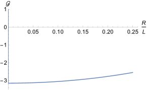
Figure 6: Shows the plot of the infinite sum in (38) as a function of $R/L$,

III Simulation details

The fluid flow satisfies the Stokes equation

$$0 =-\boldsymbol{\nabla}p+\eta\nabla^{2}\boldsymbol{v}+\boldsymbol{f}$$ (42)

$$0 =\boldsymbol{\nabla}\cdot\boldsymbol{v},$$ (43)

where,

$$\boldsymbol{f}=\boldsymbol{\nabla}\cdot(\boldsymbol{\Sigma}^{A}+\boldsymbol{\Sigma}^{E}),$$ (44)

is the force density on the fluid. The solution is obtained using Fourier transforms as we now describe.

Defining the Fourier transform of a function $\phi(\boldsymbol{r})$ as

$$\phi_{\boldsymbol{k}} =\int\phi(\boldsymbol{r})e^{-i\boldsymbol{k}\cdot\boldsymbol{r}}\,d\boldsymbol{r}$$ (45)

$$\phi(\boldsymbol{r}) =\frac{1}{(2\pi)^{3}}\int\phi_{\boldsymbol{k}}e^{i\boldsymbol{k}\cdot\boldsymbol{r}}\,d\boldsymbol{k},$$ (46)

we can write the Stokes equation (42) in the Fourier space as

$$0 =-i\boldsymbol{k}p_{\boldsymbol{k}}-\eta k^{2}\boldsymbol{v}_{\boldsymbol{k}}+\boldsymbol{f}_{\boldsymbol{k}},$$ (47)

$$0 =i\boldsymbol{k}\cdot\boldsymbol{v}_{\boldsymbol{k}}.$$ (48)

The above equations can be used to project out the solution of the pressure field in Fourier space:

$$p_{\boldsymbol{k}}=-i\frac{\boldsymbol{k}\cdot\boldsymbol{f}_{\boldsymbol{k}}}{k^{2}}.$$ (49)

The above expression of the pressure is then used in (47) to obtain the solution of the fluid flow, with built-in incompressibility, given as

$$\boldsymbol{v}_{\boldsymbol{k}} =\mathbf{G}_{\boldsymbol{k}}\cdot\boldsymbol{f}_{\boldsymbol{k}}$$ (50)

$$\mathbf{G}_{\boldsymbol{k}} =\frac{1}{\eta}\left(\frac{\boldsymbol{I}}{k^{2}}-\frac{\boldsymbol{k}\boldsymbol{k}}{k^{4}}\right).$$ (51)

Here $\mathbf{G}_{\boldsymbol{k}}$ is the Fourier transform of the Oseen tensor $\mathbf{G}(\boldsymbol{r})$ Pozrikidis (1992).

The above solution for the fluid flow is implemented using the standard fast Fourier transforms (FFTs) implemented in NumPy Oliphant (2006), which automatically implements periodic boundary condition. The remaining terms in the dynamics of the $\phi$ and $\psi$ field are implemented using using the pseudo-spectral method, involving again NumPy Fourier transforms and $2/3$ dealiasing procedure Orszag (1971); Boyd (2001). The linear terms are directly evaluated in the Fourier space, while the non-linear terms are computed in real space by inverse Fourier transforms. This is then transformed back to Fourier space to evolve the dynamical system in time using the explicit Euler-Maruyama method Kloeden and Platen (1992). We provide the parameters used in generating all the figures of the manuscript in Table 2. Finally, we explain the method used to determine the speed and centre-of-mass position of the $\phi$-droplet. Using the simulation data for the field $\phi(\boldsymbol{r},t)$, we obtain the centre-of-mass coordinate $\boldsymbol{R}^{\text{CM}}$ as

$$\boldsymbol{R}^{\text{CM}}(t)=\frac{\int\boldsymbol{r}\phi^{s}(\boldsymbol{r},t)\,d\boldsymbol{r}}{\int\phi^{s}(\boldsymbol{r},t)\,d\boldsymbol{r}},$$ (52)

where $\phi^{s}(\boldsymbol{r},t)$ is defined to be $1$ if $\phi(\boldsymbol{r},t)\geq 0$ and $0$ if $\phi(\boldsymbol{r},t)<0$. The self-propulsion velocity of the droplet is obtained using:

$$\boldsymbol{U}(t) =\frac{\int\phi^{s}(\boldsymbol{r},t)\boldsymbol{v}(\boldsymbol{r})\,d\boldsymbol{r}}{\int\phi^{s}(\boldsymbol{r},t)\,d\boldsymbol{r}}.$$ (53)

The above expression for the droplet velocity can be verified to hold by using the definition $\boldsymbol{U}(t)=d\boldsymbol{R}^{\text{CM}}(t)/dt$ and Eqs. (1-3) of the main text.

Physical parameters	Model parameters
Passive surface tension ($\gamma_{0}$) Bray (1994); Cates and Tjhung (2017)	$\gamma_{0}\simeq\sqrt{-8\kappa a^{3}/9b^{2}}$
Effective surface tension ($\gamma$) in presence of active stress Cates and Tjhung (2017); Singh and Cates (2019); Tiribocchi et al. (2015)	$\gamma=\gamma_{0}(1-\alpha\psi/\kappa)$
Ratio of active and passive surface tensions	$\gamma/\gamma_{0}=1-\alpha\psi/\kappa$
Binodal density of droplet $\phi$ Bray (1994); Cates and Tjhung (2017)	$\phi_{b}=\pm\sqrt{-a/b}$
Interfacial width of droplet $\phi$	$\xi_{\phi}\simeq\sqrt{-2\kappa/a}$
Binodal density of droplet $\psi$ Bray (1994); Cates and Tjhung (2017)	$\psi_{b}=\pm\sqrt{-a^{\prime}/b^{\prime}}$
Interfacial width of droplet $\psi$	$\xi_{\psi}\simeq\sqrt{-2\kappa^{\prime}/a^{\prime}}$
Radius of the $\phi$-droplet	$R$
Radius of the $\psi$-droplet	$0.9R$
Average thickness of the cortex ($\rho=\phi-\psi$)	$0.1R$
Reynolds number	$\text{Re}=\frac{\text{Inertial force}}{\text{Viscous force}}$
Capillary number	${\displaystyle\mathrm{Ca}=\eta U_{0}/\gamma_{0}}$

Table 1: Physical parameters and their corresponding model parameters used in this paper. See Tab:2 for values of the parameters. In this paper, we set inertial to zero, and thus, $\text{Re}=0$, while typical $\mathrm{Ca}\sim 0.001-0.01$.

Figure	System size ($L\times L$)	$R$	$\alpha$	$\beta$	$\beta^{\prime}$
2 (a)	$100\times 100$	20	0.1	0.02	0
2 (b)	$100\times 100$	20	0.1	0.02	0
2 (c)	$100\times 100$	20	0.1	0.02	0
3 (a)	$100\times 100$	12.5	varied	0.02	0
3 (b)	$100\times 100$	varied	0.2	0.02	0
4 (a)	$120\times 120$	10	0.2	0.02	0.2
4 (b)	$90\times 90$	10	0.2	0.02	0.2

Table 2: Simulation parameters used to study the self-propulsion of active droplets. Throughout the paper, the parameters of the free energy are fixed to be: $a=-b=a^{\prime}=-b^{\prime}=-1$, $\kappa=1.45$, and $\kappa^{\prime}=3$ for one droplet simulation. The simulations reported are in two space dimensions, while the analytic predictions would be maintained in higher dimensions. The parameter $\beta$ is fixed to be small and positive $\beta=0.02$ so that the $\psi$-droplet is confined inside the larger $\phi$-droplet. We keep the ratio of the radius of the two droplets fixed at $0.9$, such that $\phi$ droplet is bigger than the $\psi$ droplet. We fix the mobilities to be unity: $M^{\phi}=M^{\psi}=1$ and the viscosity to be $\eta=0.1$. The values of $L$, $R$, and $\alpha$ vary. We also define the area fraction to be $\varphi=\pi R^{2}/L^{2}$ . The time discretization is fixed to be $\Delta t=0.001$ and spatial discretization is fixed to be $\Delta x=1$.

IV Role of dipolar flow

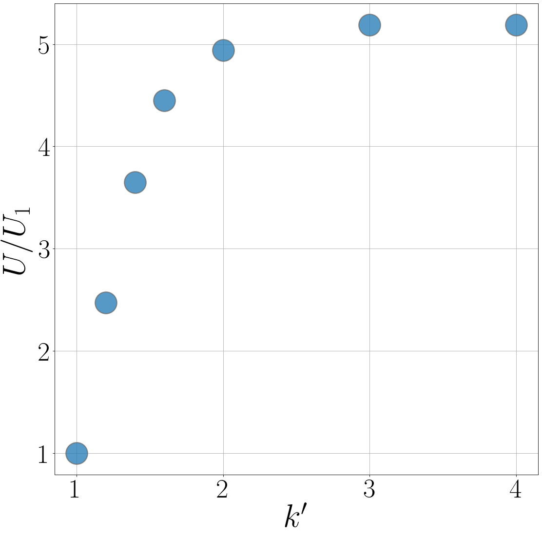
Figure 7: Speed $U$ of a droplets as the parameter $\kappa^{\prime}$ is varied. The speed is scaled by $U_{1}$, the speed for $\kappa^{\prime}=1$.

The passive stress of Eq.(4) in the main text leads to a dipolar fluid flow in presence of deformations in the $\phi$ and $\psi$ field. The deformations, in turn, are controlled by the stiffness $\kappa$ and $\kappa^{\prime}$. We use $\kappa=1.45$ to reduce deformations in the $\phi$ field. We then study the effect of changing the parameter $\kappa^{\prime}$. The dipolar flow due to deformation of the $\psi$ field impeded the droplets. In Fig.(7) we show that the speed increases as we increase the parameter $k^{\prime}$ and saturates. We choose $\kappa^{\prime}=3$ when the speed has saturated.

V Supplemental movies

The two supplemental movies are:

• Movie I: The movie corresponds to results shown in Fig.2 of the main text with the same set of parameters.

• Movie II: The movie shows dynamics of two droplets simulated using Eq.(9) of the main text. Parameters are same as in Fig.(4) but for two droplets.

References

- Marchetti et al. (2013) M. C. Marchetti, J. F. Joanny, S. Ramaswamy, T. B. Liverpool, J. Prost, Madan Rao, and R. Aditi Simha, “Hydrodynamics of soft active matter,” Reviews of Modern Physics 85, 1143–1189 (2013).
- Svitkina et al. (1997) T. M. Svitkina, A. B. Verkhovsky, K. M. McQuade, and G. G. Borisy, “Analysis of the actin–myosin II system in fish epidermal keratocytes: Mechanism of cell body translocation,” Journal of Cell Biology 139, 397–415 (1997).
- Hawkins et al. (2011) R. J. Hawkins, R. Poincloux, O. Bénichou, M. Piel, P. Chavrier, and R. Voituriez, “Spontaneous contractility-mediated cortical flow generates cell migration in three-dimensional environments,” Biophysical Journal 101, 1041–1045 (2011).
- Poincloux et al. (2011) R. Poincloux, O. Collin, F. Lizárraga, M. Romao, M. Debray, M. Piel, and P. Chavrier, “Contractility of the cell rear drives invasion of breast tumor cells in 3d matrigel,” Proceedings of the National Academy of Sciences 108, 1943–1948 (2011).
- Sanchez et al. (2012) T. Sanchez, D. T. N. Chen, S. J. DeCamp, M. Heymann, and Z. Dogic, “Spontaneous motion in hierarchically assembled active matter,” Nature 491, 431–434 (2012).
- Guillamat et al. (2018) P. Guillamat, Ž. Kos, J. Hardoüin, J. Ignés-Mullol, M. Ravnik, and F. Sagués, “Active nematic emulsions,” Science Advances 4, eaao1470 (2018).
- Tjhung et al. (2015) E. Tjhung, A. Tiribocchi, D. Marenduzzo, and M. E. Cates, “A minimal physical model captures the shapes of crawling cells,” Nature Communications 6, 5420 (2015).
- Ziebert and Aranson (2016) F. Ziebert and I. S Aranson, “Computational approaches to substrate-based cell motility,” npj Computational Materials 2, 16019 (2016).
- Camley and Rappel (2017) B. A. Camley and W. J. Rappel, “Physical models of collective cell motility: from cell to tissue,” Journal of Physics D: Applied Physics 50, 113002 (2017).
- Loisy et al. (2020) A. Loisy, J. Eggers, and T. Liverpool, “How many ways a cell can move: the modes of self-propulsion of an active drop,” Soft Matter , 3106–312 (2020).
- Tjhung et al. (2012) E. Tjhung, D. Marenduzzo, and M. E. Cates, “Spontaneous symmetry breaking in active droplets provides a generic route to motility,” Proceedings of the National Academy of Sciences 109, 12381–12386 (2012).
- Aranson (2016) Igor S. Aranson, ed., Physical Models of Cell Motility (Springer International Publishing, 2016).
- Chaikin and Lubensky (2000) P. M. Chaikin and T. C. Lubensky, Principles of condensed matter physics (Cambridge University Press, 2000).
- Cates and Tjhung (2017) M. E. Cates and E. Tjhung, “Theories of binary fluid mixtures: from phase-separation kinetics to active emulsions,” Journal of Fluid Mechanics 836, P1 (2017).
- Tiribocchi et al. (2015) A. Tiribocchi, R. Wittkowski, D. Marenduzzo, and M. E. Cates, “Active model h: Scalar active matter in a momentum-conserving fluid,” Physical Review Letters 115, 188302 (2015).
- Singh and Cates (2019) R. Singh and M. E. Cates, “Hydrodynamically interrupted droplet growth in scalar active matter,” Physical Review Letters 123, 148005 (2019).
- Blow et al. (2014) M. L. Blow, S. P. Thampi, and J. M. Yeomans, “Biphasic, lyotropic, active nematics,” Physical Review Letters 113, 248303 (2014).
- Giomi and DeSimone (2014) L. Giomi and A. DeSimone, “Spontaneous division and motility in active nematic droplets,” Physical Review Letters 112, 147802 (2014).
- (19) “See supplemental material at [to be inserted] which includes the detailed calculations, numerical method, and details of the supplemental movies.” .
- Ruprecht et al. (2015) V. Ruprecht, S. Wieser, A. Callan-Jones, M. Smutny, H. Morita, K. Sako, V. Barone, M. Ritsch-Marte, M. Sixt, R. Voituriez, and C.-P. Heisenberg, “Cortical contractility triggers a stochastic switch to fast amoeboid cell motility,” Cell 160, 673–685 (2015).
- Kim and Karrila (1991) S. Kim and S. J. Karrila, Microhydrodynamics: Principles and Selected Applications (Butterworth-Heinemann, Boston, 1991).
- Thutupalli et al. (2011) S. Thutupalli, R. Seemann, and S. Herminghaus, “Swarming behavior of simple model squirmers,” New Journal of Physics 13, 073021 (2011).
- Jin et al. (2017) C. Jin, C. Krüger, and C. C. Maass, “Chemotaxis and autochemotaxis of self-propelling droplet swimmers,” Proceedings of the National Academy of Sciences 114, 5089–5094 (2017).
- Izzet et al. (2019) A. Izzet, P. Moerman, J. Groenewold, J. Bibette, and J. Brujic, “Tunable active rotational diffusion in swimming droplets,” arXiv:1908.00581 (2019).
- Schmitt and Stark (2016) M. Schmitt and H. Stark, “Marangoni flow at droplet interfaces: Three-dimensional solution and applications,” Physics of Fluids 28, 012106 (2016).
- Leven and Newman (1976) M. D. Leven and J. Newman, “The effect of surfactant on the terminal and interfacial velocities of a bubble or drop,” AIChE Journal 22, 695–701 (1976).
- Anderson (1989) J. L. Anderson, “Colloid transport by interfacial forces,” Annu. Rev. Fluid Mech. 21, 61–99 (1989).
- Foglino et al. (2017) M. Foglino, A. N. Morozov, O. Henrich, and D. Marenduzzo, “Flow of deformable droplets: Discontinuous shear thinning and velocity oscillations,” Physical Review Letters 119, 208002 (2017).
- Ramaswamy (2001) S. Ramaswamy, “Issues in the statistical mechanics of steady sedimentation,” Advances in Physics 50, 297–341 (2001).
- Yabunaka et al. (2012) S. Yabunaka, T. Ohta, and N. Yoshinaga, “Self-propelled motion of a fluid droplet under chemical reaction,” The Journal of Chemical Physics 136, 074904 (2012).
- Fadda et al. (2017) F. Fadda, G. Gonnella, A. Lamura, and A. Tiribocchi, “Lattice boltzmann study of chemically-driven self-propelled droplets,” The European Physical Journal E 40, 112 (2017).
- Morozov and Michelin (2019a) M. Morozov and S. Michelin, “Nonlinear dynamics of a chemically-active drop: From steady to chaotic self-propulsion,” The Journal of Chemical Physics 150, 044110 (2019a).
- Lavi et al. (2020) I. Lavi, N. Meunier, R. Voituriez, and J. Casademunt, “Motility and morphodynamics of confined cells,” Phys. Rev. E 101, 022404 (2020).
- Thutupalli et al. (2018) S. Thutupalli, D. Geyer, R. Singh, R. Adhikari, and H. A. Stone, “Flow-induced phase separation of active particles is controlled by boundary conditions,” Proceedings of the National Academy of Sciences 115, 5403–5408 (2018).
- Morozov and Michelin (2019b) M. Morozov and S. Michelin, “Self-propulsion near the onset of marangoni instability of deformable active droplets,” J. Fluid Mech. 860, 711–738 (2019b).
- Lohse and Zhang (2020) D. Lohse and X. Zhang, “Physicochemical hydrodynamics of droplets out of equilibrium: A perspective review,” arXiv preprint arXiv:2005.03782 (2020).
- Yamamoto and Sano (2017) T. Yamamoto and M. Sano, “Chirality-induced helical self-propulsion of cholesteric liquid crystal droplets,” Soft Matter 13, 3328–3333 (2017).
- Shaebani et al. (2020) M. R. Shaebani, A. Wysocki, R. G. Winkler, G. Gompper, and H. Rieger, “Computational models for active matter,” Nature Rev. Phys. , 1–19 (2020).
- Happel and Brenner (1981) J. Happel and H. Brenner, Low Reynolds number hydrodynamics (Springer Netherlands, 1981).
- Brady et al. (1988) J. F. Brady, R. J. Phillips, J. C. Lester, and G. Bossis, “Dynamic simulation of hydrodynamically interacting suspensions,” Journal of Fluid Mechanics 195, 257–280 (1988).
- O’brien (1979) R. W. O’brien, “A method for the calculation of the effective transport properties of suspensions of interacting particles,” Journal of Fluid Mechanics 91, 17–39 (1979).
- Pozrikidis (1992) C. Pozrikidis, Boundary Integral and Singularity Methods for Linearized Viscous Flow (Cambridge University Press, 1992).
- Oliphant (2006) T. E. Oliphant, Guide to NumPy (CreateSpace Independent Publishing Platform; 2nd edition, 2006).
- Orszag (1971) S. A. Orszag, “Accurate solution of the orr–sommerfeld stability equation,” Journal of Fluid Mechanics 50, 689–703 (1971).
- Boyd (2001) J. P. Boyd, Chebyshev and Fourier Spectral Methods: Second Revised Edition (Dover Publications; Second Edition, 2001).
- Kloeden and Platen (1992) P. E. Kloeden and E. Platen, Numerical Solution of Stochastic Differential Equations (Springer Berlin Heidelberg, 1992).
- Bray (1994) A. J. Bray, “Theory of phase-ordering kinetics,” Adv. Phys. 43, 357 (1994).