Heavy-hadron molecules from light-meson-exchange saturation

Abstract

In the effective field theory framework the interaction between two heavy hadrons can be decomposed into a long- and a short-range piece. The long-range piece corresponds to the one-pion-exchange potential and is relatively well-known. The short-range piece is given by a series of contact-range interactions with unknown couplings, which substitute the less well-known short-range dynamics. While the general structure of the short-range potential between heavy hadrons is heavily constrained from heavy-quark symmetry, the couplings are still free parameters. Here we argue that the relative strength and the sign of these couplings can be estimated from the hypothesis that they are saturated by the exchange of light mesons, in particular the vector mesons $\rho$ and $\omega$, i.e. from resonance saturation. However, we propose a novel saturation procedure that effectively removes form-factor artifacts. From this we can determine in which spin and isospin configurations the low-energy constants are most attractive for specific two-heavy-hadron systems. In general the molecular states with lower isospins and higher spins will be more attractive and thus more probable candidates to form heavy-hadron molecules. This pattern is compatible with the interpretation of the $X(3872)$ and $P_{c}(4312/4440/4457)$ as molecular states, but it is not applicable to states with maximum isospin like the $Z_{c}(3900/4020)$.

Heavy-hadron molecules might very well be the most popular type of exotic hadron Voloshin and Okun (1976); De Rujula et al. (1977); Guo et al. (2018). The probable reason is their conceptual simplicity, which is only matched by the challenge of making concrete predictions in the molecular picture. Despite just being non-relativistic bound states of two heavy hadrons, the theoretical toolbox behind hadronic molecules has grown into a bewildering hodgepodge which is often difficult to disentangle, to say the least. This is in contrast with the much more coherent descriptions offered by the quark model Godfrey and Isgur (1985); Capstick and Isgur (1986) or the theory behind quarkonium Eichten et al. (1978, 1980); Brambilla et al. (2000, 2005, 2011).

Yet the molecular picture has a few remarkable successes under its sleeves. They include the prediction of the $X(3872)$ by Törnqvist Tornqvist (1994), later detected by the Belle collaboration Choi et al. (2003), and the prediction of three hidden-charm pentaquarks Wu et al. (2010, 2011); Wu and Zou (2012); Xiao et al. (2013); Wang et al. (2011); Yang et al. (2012); Karliner and Rosner (2015) ($\Sigma_{c}\bar{D}$ and $\Sigma_{c}\bar{D}^{*}$ molecules), which might very well correspond with the $P_{c}(4312)$, $P_{c}(4440)$ and $P_{c}(4457)$ pentaquarks recently detected by the LHCb Aaij et al. (2019). Regarding the $X(3872)$, the most compelling evidence that it is molecular is not necessarily its closeness to the $D^{*}\bar{D}$ threshold Tornqvist (2003); Voloshin (2004); Braaten and Kusunoki (2004) but its isospin-breaking decays Choi et al. (2011) which are naturally reproduced in the molecular picture Gamermann and Oset (2009); Gamermann et al. (2010) (in the non-molecular case this feature might Swanson (2004) or might not be explainable Hanhart et al. (2011) depending on the details of the model). For the LHCb pentaquarks, though the molecular explanation is gaining traction Roca et al. (2015); He (2016); Xiao and Meißner (2015); Chen et al. (2015a, b); Burns (2015); Geng et al. (2018); Chen et al. (2019a, b); Liu et al. (2018, 2019a); Xiao et al. (2019); Pavon Valderrama (2019a); Burns and Swanson (2019); Pan et al. (2019); Du et al. (2020), there are a few competing hypotheses about their nature Eides et al. (2019); Wang (2020); Cheng and Liu (2019).

Despite the numerous candidates and the intense theoretical interest, the qualitative and quantitative properties of the molecular spectrum are poorly understood. The present manuscript attempts to address this limitation by proposing a potential pattern in the spectrum of two-heavy-hadron bound states: for configurations without maximum isospin, the states with higher (light-quark) spin are expected to be lighter (i.e. more bound). This is the opposite pattern as with compact hadrons, for which mass usually increases with spin. This pattern might explain why besides the $X(3872)$ no other $D^{(*)}\bar{D}^{(*)}$ molecule has been observed, as they should not be expected to be bound (with the exception of the $2^{++}$ $D^{*}\bar{D}^{*}$ configuration Valderrama (2012); Nieves and Valderrama (2012), modulo other effects that could unbind it Cincioglu et al. (2016); Baru et al. (2016)). If applied to the light sector, it also explains why in the two-nucleon system the deuteron binds while the singlet state does not, or why if the $d^{*}(2380)$ Adlarson et al. (2011) is a $\Delta\Delta$ bound state Dyson and Xuong (1964) its spin should be $J=3$. It also states that if the $P_{c}(4440)$ and $P_{c}(4457)$ are $\Sigma_{c}\bar{D}^{*}$ bound states, their expected quantum numbers are $\tfrac{3}{2}^{-}$ and $\tfrac{1}{2}^{-}$, respectively. This prediction, which agrees with a few theoretical analyses Pavon Valderrama (2019a); Liu et al. (2019b); Du et al. (2020), will be put to the test by the eventual experimental determination of the quantum numbers of the pentaquarks.

This pattern is deduced from matching a contact-range description of the interaction between two heavy hadrons with a phenomenological description in terms of the potential generated by the exchange of light mesons. That is, we are considering the saturation of the low-energy constants by light-meson exchange (as in Refs. Ecker et al. (1989); Epelbaum et al. (2002)). We will illustrate this idea with the one-pion-exchange (OPE) potential, which for two spin-$\tfrac{1}{2}$, isospin-$\tfrac{1}{2}$ hadrons reads

$$V(\vec{q}\,) = -\frac{g^{2}}{2f^{2}}\,{\tau}\,\frac{\vec{\sigma}_{1}\cdot\vec{q}\,\vec{\sigma}_{2}\cdot\vec{q}}{q^{2}+m_{\pi}^{2}}$$

$$= -\frac{g^{2}}{2f^{2}}\,{\tau}\,\left[\frac{\frac{1}{3}\,\vec{\sigma}_{1}\cdot\vec{\sigma}_{2}q^{2}}{q^{2}+m_{\pi}^{2}}+\frac{\vec{\sigma}_{1}\cdot\vec{q}\,\vec{\sigma}_{2}\cdot\vec{q}-\frac{1}{3}\vec{\sigma}_{1}\cdot\vec{\sigma}_{2}q^{2}}{q^{2}+m_{\pi}^{2}}\right]\,,$$

with $g$ the axial coupling, $f\sim 130\,{\rm MeV}$ the pion decay constant, $\vec{q}$ the exchanged momentum and $q=|\vec{q}\,|$, $m_{\pi}$ the pion mass, $\vec{\sigma}_{i}$ ($\bm{\tau}_{i}$) the Pauli matrices for hadron $i=1,2$ in spin (isospin) space, and $\tau=\bm{\tau}_{1}\cdot\bm{\tau}_{2}$ an isospin factor. In the second line the potential has been decomposed into a spin-spin and a tensor piece. We will ignore the tensor piece, as it requires SD-wave mixing. We will consider the effect of OPE on the saturation of the couplings of the lowest-order contact-range potential, which is purely S-wave. Finally we will ignore the practical and theoretical considerations derived from the fact that the pion is the lightest hadron (namely chiral symmetry): obviously under most settings we are not interested in saturation by pions, but in saturation by scalar- and vector-meson exchange. The choice of pions is merely intended as a simple example of the mechanics of saturation.

The idea behind saturation is to map the previous finite-range potential into an effective potential of the type

$$V_{C}(\vec{q}\,)=C_{0}(\mu)+C_{1}(\mu)\,\vec{\sigma}_{1}\cdot\vec{\sigma}_{2}\,,$$ (2)

which requires a regulator (not explicitly written here), with $\mu$ being a regularization scale (i.e. a cutoff), which we will choose around the mass of the exchanged light meson ($\mu\sim m_{\pi}$ in this case) for saturation to work. If we expand the spin-spin piece of Eq. (LABEL:eq:OPE) in powers of $q$,

$$V(\vec{q}\,)=-\frac{g^{2}}{6f^{2}}\,\tau\,\vec{\sigma}_{1}\cdot\vec{\sigma}_{2}\left[\frac{q^{2}}{m_{\pi}^{2}}-\frac{q^{4}}{m_{\pi}^{4}}+\dots\right]\,,$$ (3)

then, by matching this expansion with the effective potential $V_{C}$, we will deduce that OPE should not saturate the couplings:

$$C^{\rm OPE}_{0}(\mu\sim m_{\pi})\sim 0\,,\quad C^{\rm OPE}_{1}(\mu\sim m_{\pi})\sim 0\,.$$ (4)

However this conclusion is premature. If we rewrite the $q^{2}$-dependence as

$$\frac{q^{2}}{q^{2}+m_{\pi}^{2}}=1-\frac{m_{\pi}^{2}}{q^{2}+m_{\pi}^{2}}\,,$$ (5)

then the first contribution in the right-hand side is actually a Dirac delta. Owing to the finite size of the pions, this Dirac delta will acquire a finite size $\sim 1/M$, with $M$ the physical cutoff of the theory (probably a bit above $1\,{\rm GeV}$). This does not necessarily coincide with the scale $\mu$ we use for the effective interaction. In general saturation works best for $\mu\sim m$ with $m$ the mass of the light meson, while for the exchange of a light meson to have physical meaning we need $m<M$. From this the saturation scale verifies $\mu<M$, implying that in practice we can simply ignore contributions with a range shorter than $1/\mu$ ($\sim 1/m$), including the aforementioned delta. Thus for saturation purposes we will simply make the substitution

$$\frac{q^{2}}{q^{2}+m_{\pi}^{2}}\to-\frac{m_{\pi}^{2}}{q^{2}+m_{\pi}^{2}}\,,$$ (6)

in the exchange potential, leading to

$$V(\vec{q}\,) \to \frac{g^{2}}{6f^{2}}\,{\tau}\,\frac{\vec{\sigma}_{1}\cdot\vec{\sigma}_{2}\,m_{\pi}^{2}}{q^{2}+m_{\pi}^{2}}+\dots\,,$$ (7)

where the dots represent terms mixing S- and D-waves. Matching at $q^{2}=0$, we obtain the saturated couplings:

$$C^{\rm OPE}_{0}(\mu\sim m_{\pi})\sim 0\,,\quad C^{\rm OPE}_{1}(\mu\sim m_{\pi})\sim\frac{g^{2}}{6f^{2}}\,\tau\,.$$ (8)

Finally we can compare how well does the saturated contact-range interaction versus the potential from which it is derived. This is done in Fig. 1, where we check that it works relatively well for the scattering length $a_{0}$ as a function of the strength of the potential (see Appendix A for supplementary details). Particularly saturation correctly reproduces the existence of a bound state, which is signaled by a change of sign in $1/a_{0}$.

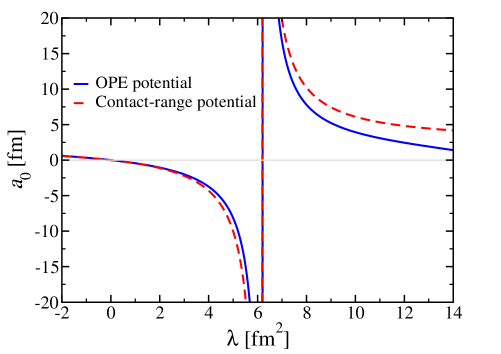
Figure 1: Scattering length $a_{0}$ (in fm) for the S-wave piece of the OPE potential and for the S-wave contact-range of Eq. (2) with the saturation conditions of Eq. (8) and a regularization scale $\mu=131\,{\rm MeV}$ (close to the pion mass). We plot $a_{0}$ as a function of the strength of the potential $\lambda=-\tau g^{2}/6f^{2}\vec{\sigma}_{1}\cdot\vec{\sigma}_{2}$. The contact-range potential is regularized with a separable sharp-cutoff regulator in momentum space, i.e. $\braket{\vec{p}\,^{\prime}}{V_{C}}{\vec{p}\,}=(C_{0}+C_{1}\,\vec{\sigma}_{1}\cdot\vec{\sigma}_{2})\,\theta\left({{{\mu-p^{\prime}}}}\right)\theta\left({{{\mu-p}}}\right)$.

As previously noted, the saturation of low-energy couplings by OPE serves an illustrative purpose. Its practical value is limited: owing to chiral symmetry the pion mass is considerably lower than any other hadronic scales. In most practical settings, pion exchanges will be included explicitly as the finite-range potential, while the contact-range potential will be saturated by scalar- and vector-meson exchange. Pion saturation might be useful for the few hadronic molecules in which all the relevant momentum scales are lighter than the pion. With the exception of the deuteron (or, more generally, few-nucleon systems) and the $X(3872)$, which can be described in terms of a pionless EFT van Kolck (1999); Chen et al. (1999); Braaten and Kusunoki (2004); Fleming et al. (2007), most hadronic molecules do not fall into this category Valderrama (2012); Lu et al. (2019) (and even the few that fall might still benefit from a pionful treatment). Therefore the problem is to apply saturation to other light mesons, in particular the sigma, the rho and the omega.

We will now explain the concrete application of saturation to heavy-hadron molecules. Instead of using the standard superfield formalism we will write the interaction between two heavy hadrons in the light-quark formalism described in Ref. Pavon Valderrama (2019b) (see Appendix B for a more detailed explanation). This formalism merely amounts to notice that in the heavy-quark limit interactions among heavy hadrons do not depend on heavy-quark spin, which means that all spin dependence can be rewritten in terms of the spin degrees of freedom of the light quarks within the heavy hadrons. The number of independent contact-range couplings depends on the ways to combine the light spins $S_{L1}$ and $S_{L2}$ of the two heavy hadrons $1$ and $2$: $S_{L1}\otimes S_{L2}=|S_{L1}-S_{L2}|\oplus\ldots\oplus(S_{L1}+S_{L2})$. This means, for instance, that in the $D\bar{D}$ and $\Sigma_{c}\bar{D}$ families of molecules there are two independent couplings, in the $\Sigma_{c}\Sigma_{c}$ family three independent couplings and in the $D_{1}\bar{D}_{1}$ family four couplings. In addition, if the two heavy hadrons have different light spin, there is the possibility of additional couplings from operators involving the exchange of light spin (the $\Lambda_{c}\Sigma_{c}$ system being an example). From this the S-wave contact-range interaction of two heavy hadrons can be written as

$$V_{C}=C_{0}+C_{1}\,\hat{S}_{L1}\cdot\hat{S}_{L2}+C_{2}\,\hat{Q}_{L1,ij}\hat{Q}_{L2,ij}+\dots,$$ (9)

that is, a series of the products of irreducible tensors built from the light-spin operators $\vec{S}_{L1}$ and $\vec{S}_{L2}$. The operator $\hat{S}_{L}=\vec{S}_{L}/|\vec{S}_{L}|$ is a normalized spin operator, while the operator $\hat{Q}_{L,ij}$ is the spin-2 product

$$Q_{L,ij}=\frac{1}{2}\left[S_{L,i}S_{L,j}+S_{L,j}S_{L,i}\right]-\frac{\vec{S}_{L}^{2}}{3}\delta_{i,j}\,,$$ (10)

which is later normalized as $\hat{Q}_{L,ij}=Q_{L,ij}/|Q_{L,33}|$. Analogously we can define higher-spin products of $S_{L1}$ and $S_{L2}$.

To determine how to saturate the couplings $C_{J}$ of the effective potential, we will split it in two contributions coming from the scalar- and vector-meson potentials: $C_{J}=C_{J}^{S}+C^{V}_{J}$. We begin by writing the Lagrangians. For the interaction of a scalar meson with the light-quark degrees of freedom, the Lagrangian reads

$$\mathcal{L}^{S}=g_{\sigma}\,{q}_{L}^{\dagger}\sigma\,q_{L}\,,$$ (11)

where $g_{\sigma}$ is a coupling constant, $\sigma$ is the scalar meson field and $q_{L}$ is a non-relativistic field with the quantum numbers of the light quarks within the heavy hadron, i.e. instead of writing down the full heavy-hadron field, what we are using is an effective field that only contains the degrees of freedom that are relevant for describing interactions among heavy hadrons. With this Lagrangian we end up with the potential

$$V_{\sigma}=-\frac{g_{\sigma}^{2}}{q^{2}+m_{\sigma}^{2}}\,,$$ (12)

for which saturation reads

$$C^{S}_{0}\sim-\frac{g_{\sigma}^{2}}{m_{\sigma}^{2}}\,,\quad C^{S}_{J\geqslant 1}\sim 0\,.$$ (13)

For the vector mesons the Lagrangian can be written as the multipole expansion

$$\mathcal{L}^{V}= \,\mathcal{L}^{V}_{E0}+\mathcal{L}^{V}_{M1}+\mathcal{L}^{V}_{E2}+\dots$$

$$= \,g_{V}\,{q}_{L}^{\dagger}V_{0}q_{L}+\frac{f_{V}}{2M}\,q_{L}^{\dagger}\,\hat{S}_{L}\cdot(\vec{\nabla}\times\vec{V})\,q_{L}$$ (14)

$$+\,\frac{h_{V}}{2M^{2}}\,{q_{L}}^{\dagger}\,\hat{Q}_{L{\color[rgb]{0,0,1},}ij}\,\partial_{i}\partial_{j}V_{0}\,q_{L}+\dots\,,$$

where we have explicitly written the electric charge, magnetic dipole and electric quadrupolar terms and with the dots indicating higher-order multipole terms. In this Lagrangian, $g_{V}$, $f_{V}$ and $h_{V}$ are coupling constants, $V_{\mu}=(V_{0},\vec{V}\,)$ is the vector meson field and $M$ is the typical mass scale associated to the size of the vector mesons. The number of terms depends on the spin of the light-quark degrees of freedom, where for $S_{L}=0$ (e.g. $\Lambda_{c}$) there is only the electric term, for $S_{L}=\frac{1}{2}$ (e.g. $D$, $D^{*}$) there is also the magnetic dipole term, for $S_{L}=1$ ($\Sigma_{c}$, $\Sigma_{c}^{*}$) we add the electric quadrupole term, and so on. From this Lagrangian it is easy to derive the one-boson-exchange potential Machleidt et al. (1987) for a particular two-heavy-hadron system, where the contributions read

$$V_{E0} = +\frac{g_{V}^{2}}{q^{2}+m_{V}^{2}}\,,$$ (15)

$$V_{M1} = -\frac{f_{V}^{2}}{4M^{2}}\,\frac{(\hat{S}_{L1}\times\vec{q}\,)\cdot(\hat{S}_{L2}\times\vec{q}\,)}{q^{2}+m_{V}^{2}}$$ (16)

$$= -\frac{2}{3}\,\frac{f_{V}^{2}}{4M^{2}}\,\hat{S}_{L1}\cdot\hat{S}_{L2}\,\frac{q^{2}}{q^{2}+m_{V}^{2}}+\dots\,,$$

$$V_{E2} = +\frac{h_{V}^{2}}{4M^{4}}\,\frac{(\hat{Q}_{L1,ij}\,q_{i}q_{j})\,(\hat{Q}_{L2,lm}\,q_{l}q_{m})}{q^{2}+m_{V}^{2}}$$ (17)

$$= +\frac{h_{V}^{2}}{36M^{4}}\,(\hat{Q}_{L1,ij}\hat{Q}_{L2,ij})\,\frac{q^{4}}{q^{2}+m_{V}^{2}}+\dots\,,$$

where for the M1 and E2 terms we isolate the S-wave piece in the second line. If we remove the Dirac-delta terms, we can deduce the saturation condition for vector-meson exchange. But first we have to distinguish between the $\omega$ and $\rho$ meson contributions. The most obvious difference is that the $\rho$ contribution contains an isospin factor that we have not explicitly written. Owing to the negative G-parity of the $\omega$, its contribution changes sign depending on whether we are dealing with a hadron-hadron or hadron-antihadron system. Regarding the couplings, SU(3)-flavor symmetry and the OZI rule imply that the $\rho$ and $\omega$ couplings are identical for heavy hadrons in the $3$ or $6$ representation (which include all the cases considered here). After removing the Dirac-delta terms, we get the saturation conditions

$$C_{0}^{V}(\mu\sim m_{V}) \sim \frac{g_{V}^{2}}{m_{V}^{2}}\,(\zeta+\bm{\hat{T}}_{1}\cdot\bm{\hat{T}}_{2})\,,$$ (18)

$$C_{1}^{V}(\mu\sim m_{V}) \sim \frac{f_{V}^{2}}{6M^{2}}\,(\zeta+\bm{\hat{T}}_{1}\cdot\bm{\hat{T}}_{2})\,,$$ (19)

$$C_{2}^{V}(\mu\sim m_{V}) \sim \frac{h_{V}^{2}m_{V}^{2}}{36M^{4}}\,(\zeta+\bm{\hat{T}}_{1}\cdot\bm{\hat{T}}_{2})\,,$$ (20)

where $\zeta=\pm 1$ gives the contribution from the omega and $\bm{\hat{T}}_{i}=\bm{T}_{i}/T_{i}$ is the normalized isospin operator. The saturation condition generates $C_{J}$ couplings with consistent signs. From this we can see that for the isoscalar hadron-antihadron system the saturated couplings are always attractive:

$$C_{J}^{V}(I<I_{1}+I_{2})<0\,.$$ (21)

This does not imply that the potential is always attractive, because that will depend on the linear combination of $C_{J}$’s that conform the contact-range potential in a given channel. Yet, if we notice that the $C_{J}$’s follow a multipole expansion, the natural expectation is that terms involving higher multipoles will be smaller:

$$|C_{J^{\prime}}^{V}|<|C_{J}^{V}|\quad\mbox{for $J^{\prime}>J$.}$$ (22)

This expectation is indeed confirmed by the LHCb pentaquark trio, provided they are molecular, as attested by a few theoretical works Liu et al. (2018, 2019a); Pavon Valderrama (2019a); Du et al. (2020).

Molecule	$J^{P}$	$V$	Attractive?
$D\bar{D}$	$0^{++}$	$C_{0}$	Yes
$D^{*}\bar{D}$	$1^{++}$	$C_{0}+C_{1}$	Most
$D^{*}\bar{D}$	$1^{+-}$	$C_{0}-C_{1}$	Likely
$D^{*}\bar{D}^{*}$	$0^{++}$	$C_{0}-2C_{1}$	Likely
$D^{*}\bar{D}^{*}$	$1^{+-}$	$C_{0}-C_{1}$	Likely
$D^{*}\bar{D}^{*}$	$2^{++}$	$C_{0}+C_{1}$	Most
Molecule	$J^{P}$	$V$	Attractive?
$\bar{D}\Sigma_{c}$	$\frac{1}{2}^{-}$	$D_{0}$	Yes
$\bar{D}\Sigma_{c}^{*}$	$\frac{3}{2}^{-}$	$D_{0}$	Yes
$\bar{D}^{*}\Sigma_{c}$	$\frac{1}{2}^{-}$	$D_{0}-\frac{4}{3}\,D_{1}$	Likely
$\bar{D}^{*}\Sigma_{c}$	$\frac{3}{2}^{-}$	$D_{0}+\frac{2}{3}\,D_{1}$	Most
$\bar{D}^{*}\Sigma_{c}^{*}$	$\frac{1}{2}^{-}$	$D_{0}-\frac{5}{3}\,D_{1}$	Likely
$\bar{D}^{*}\Sigma_{c}^{*}$	$\frac{3}{2}^{-}$	$D_{0}-\frac{2}{3}\,D_{1}$	Likely
$\bar{D}^{*}\Sigma_{c}^{*}$	$\frac{5}{2}^{-}$	$D_{0}+D_{1}$	Most
Molecule	$J^{P}$	$V$	Attractive?
$\Sigma_{c}\bar{\Sigma}_{c}$	$0^{-+}$	$E_{0}-\frac{4}{3}E_{1}$	Likely
$\Sigma_{c}\bar{\Sigma}_{c}$	$1^{--}$	$E_{0}+\frac{4}{9}E_{1}$	Yes
$\Sigma_{c}^{*}\bar{\Sigma}_{c}$	$1^{-+}$	$E_{0}-E_{1}-\frac{15}{2}E_{2}$	Likely
$\Sigma_{c}^{*}\bar{\Sigma}_{c}$	$1^{--}$	$E_{0}-\frac{11}{9}E_{1}+\frac{15}{2}E_{2}$	Likely
$\Sigma_{c}^{*}\bar{\Sigma}_{c}$	$2^{-+}$	$E_{0}+\frac{1}{3}E_{1}-\frac{3}{2}E_{2}$	Likely
$\Sigma_{c}^{*}\bar{\Sigma}_{c}$	$2^{--}$	$E_{0}+E_{1}+\frac{3}{2}E_{2}$	Most
$\Sigma_{c}^{*}\bar{\Sigma}_{c}^{*}$	$0^{-+}$	$E_{0}-\frac{15}{9}E_{1}+\frac{15}{2}E_{2}$	Likely
$\Sigma_{c}^{*}\bar{\Sigma}_{c}^{*}$	$1^{--}$	$E_{0}-\frac{11}{9}E_{1}+\frac{3}{2}E_{2}$	Likely
$\Sigma_{c}^{*}\bar{\Sigma}_{c}^{*}$	$2^{-+}$	$E_{0}-\frac{1}{3}E_{1}-\frac{9}{2}E_{2}$	Likely
$\Sigma_{c}^{*}\bar{\Sigma}_{c}^{*}$	$3^{--}$	$E_{0}+E_{1}+\frac{3}{2}E_{2}$	Most

Table 1: Structure of the contact-range potential for the $\bar{D}D$, $\bar{D}\Sigma_{c}$ and $\bar{\Sigma}_{c}\Sigma_{c}$ family of molecules. For configurations in which the isospin $I$ of the molecule is not maximal, $I<I_{1}+I_{2}$, all the couplings appearing in this table are expected to be negative in sign (i.e. attractive). If we take into account that the previous couplings are expected to be smaller as the multipole moment increases, then we arrive at the labels “Most”, “Yes”, “Likely” to characterize whether a particular molecular configuration is attractive.

To illustrate this idea we consider a few examples: (1) the $DD$ and $D\bar{D}$ family of molecules, (2) the $D\Sigma_{c}$ and $\bar{D}\Sigma_{c}$ family, and (3) the $\Sigma_{c}\Sigma_{c}$ and $\Sigma_{c}\bar{\Sigma}_{c}$ one. We have summarized the form of the contact-range potential for these three cases in Table 1. For the first case, which includes the $X(3872)$, it is more convenient to define the contact-range potential in terms of the Pauli matrices (instead of the spin matrices)

$$V_{c}^{(1)}=C_{0}+\vec{\sigma}_{L1}\cdot\vec{\sigma}_{L2}\,C_{1}\,,$$ (23)

for which vector saturation gives

$$C_{0}^{V} \sim \frac{g_{V}^{2}}{m_{V}^{2}}(\zeta+\bm{\tau}_{1}\cdot\bm{\tau}_{2})\,,$$ (24)

plus the analogous expression for $C_{1}^{V}$. From this it is clear that the $I=0$ isoscalar configurations are guaranteed to be attractive. For the isovector configurations the $\rho$ and $\omega$ contributions cancel out: for the $C_{0}$ coupling there is still the scalar-meson contribution, which will result in attraction, while for the $C_{1}$ coupling the sign will depend on how the SU(3)-flavor symmetry is broken. Alternatively, the exchange of the $a_{1}$ meson Durso et al. (1984) would imply $C_{1}(I_{1}=1)\geqslant 0$ for the $Z_{c}(3900)$ and $Z_{c}(4020)$ resonances, which is compatible with their quantum numbers ($J^{PC}=1^{+-}$). Thus it might be possible that the $I=I_{1}+I_{2}$ configurations revert to the naive expectation of higher (light-quark) spin states having higher masses.

For the second case, the $\bar{D}\Sigma_{c}$ and $D\Sigma_{c}$ family of molecules (which include the LHCb pentaquark trio), we define the contact-range potential as

$$V_{C}^{(2)}=D_{0}+\vec{\sigma}_{L1}\cdot\vec{S}_{L2}\,D_{1}\,,$$ (25)

where $\vec{S}_{L2}$ refers to the spin-1 angular momentum matrices. Saturation in this case gives

$$D_{0}^{V} \sim \frac{g_{V}g_{V}^{\prime}}{m_{V}^{2}}(\zeta+\bm{\tau}_{1}\cdot\bm{T}_{2})\,,$$ (26)

plus the analogous expression for $D_{1}$, with $g_{V}^{\prime}$ the vector-meson coupling for the $\Sigma_{c}$ and $\Sigma_{c}^{*}$ baryons and $\bm{T}_{2}$ their isospin operators. This expression indicates that the isospin-$\frac{1}{2}$ configurations are attractive for both the $\bar{D}\Sigma_{c}$ and $D\Sigma_{c}$ cases. A second conclusion is that in the $\bar{D}^{*}\Sigma_{c}$ system the $J^{P}=\tfrac{3}{2}^{-}$ configuration is expected to be more attractive than the $J^{P}=\tfrac{1}{2}^{-}$ one, which implies that the quantum numbers of the $P_{c}(4440)$ and $P_{c}(4457)$ pentaquarks should be $J^{P}=\tfrac{3}{2}^{-}$ and $\tfrac{1}{2}^{-}$, respectively. A third conclusion is that the doubly charmed ${D}\Sigma_{c}$-type family of molecules are expected to be more tightly bound than the hidden-charm pentaquarks, owing to the different sign of the $\omega$ contribution Yu et al. (2019).

Finally, if we apply it to the $\Sigma_{c}\Sigma_{c}$ and $\Sigma_{c}\bar{\Sigma}_{c}$ family of molecules, the contact-range potential reads

$$V_{C}^{(3)}=E_{0}+E_{1}\,\vec{S}_{L1}\cdot\vec{S}_{L2}+E_{2}\,\hat{Q}_{L1,ij}\hat{Q}_{L2,ij}\,.$$ (27)

The vector-meson saturation of the couplings yields

$$E_{0} \sim \frac{g_{V}^{\prime 2}}{m_{V}^{2}}(\zeta+\bm{T}_{1}\cdot\bm{T}_{2})\,,$$ (28)

plus the analogous expressions for $E_{1}$ and $E_{2}$. From this the isoscalar and isovector $2^{--}$ and $3^{--}$ heavy baryonia are expected to be the most attractive.

We stress the qualitative character of the present analysis. Saturation requires two conditions for the regularization scale $\mu$: it must be close to the mass of the exchanged meson $m$ and it must be (ideally much) softer than the physical cutoff $M$, i.e. $\mu\sim m$ and $\mu<M$ (even better: $\mu\ll M$). Though these two conditions are indeed met for scalar- and vector-meson exchange, the ratio $\mu/M$ is not small, which indicates that the saturation of the couplings is not necessarily expected to do well quantitatively. However previous investigations on the couplings in the pion-nucleon Ecker et al. (1989) and nucleon-nucleon Epelbaum et al. (2002) systems indicate that contact-range couplings are indeed saturated by light-meson exchange. We do not know whether this will be the case for hadronic molecules, yet the present manuscript focuses on the qualitative aspects of saturation, particularly the signs of the couplings, which are more likely to be unaffected by the poor scale separation.

To summarize, we propose a description of heavy-hadron molecules in terms of contact-range potentials that depend on a few couplings. The couplings are determined from saturation by scalar- and vector-meson exchange, where we propose a novel saturation procedure that takes into account the physical scale at which saturation is actually happening. The outcome is that it is possible to know the sign and relative strength of the two-heavy-hadron interaction, from which we can deduce a few qualitative properties of the heavy molecular spectrum. The most interesting pattern is that for heavy molecular states without maximal isospin, we expect the configurations with higher light-quark spin to be more bound (or, equivalently, lighter if we refer to the mass of the states). This pattern is exactly the opposite of the one that is observed in standard compact hadrons, where mass usually increases with spin. The pattern is compatible with the quantum numbers of the $X(3872)$ in the molecular picture and with the experimental absence of molecular partners of the $X(3872)$ with smaller light-quark spin. The pattern also extends to the light sector, with the deuteron (neutron-proton, $I(J)=0(1)$) and the recently observed $d^{*}(2380)$ ($\Delta\Delta$, $I(J)=0(3)$) being two illustrative examples. Yet the real test of the present idea will be the eventual experimental measurement of the quantum numbers of the $P_{c}(4440)$ and $P_{c}(4457)$ pentaquarks. If they are $\bar{D}^{*}\Sigma_{c}$ molecules, the saturation hypothesis suggests that the $J=\tfrac{3}{2}$ state should be the most bound of the two, i.e. the spin of the $P_{c}(4440)$ should be $\tfrac{3}{2}$.

Appendix A Scattering length and saturation in a contact-range theory

Here we explain the calculation of the scattering length $a_{0}$ and the choice of the regularization scale $\mu$ that we have presented in Fig. 1. First we explicitly regularize the contact-range potential of Eq. (2), i.e.

$$\braket{\vec{p}{\,{}^{\prime}}}{V^{R}_{C}}{\vec{p}\,} = f_{R}(p^{\prime}/\mu)\,\left[C_{0}(\mu)+C_{1}(\mu)\,\vec{\sigma}_{1}\cdot\vec{\sigma}_{2}\right]\,f_{R}(p/\mu)\,,$$

where we have chosen a generic non-local regulator $f_{R}(x)$ such that $f_{R}(0)=1$ and $f_{R}(x\to\infty)\to 0$. For obtaining the scattering matrix $T$, we insert the regularized contact-range potential $V_{C}^{R}$ in the Lippmann-Schwinger equation

$$T(E_{\rm cm})=V_{C}^{R}+V_{C}^{R}\,G_{0}(E_{\rm cm})\,T(E_{\rm cm})\,,$$ (30)

with $E_{\rm cm}$ the center-of-mass energy of the two-body system and $G_{0}(E_{\rm cm})=1/(E_{\rm cm}-H_{0})$ the resolvent operator, $H_{0}$ being the free Hamiltonian (i.e. the kinetic energy operator). As we are interested in the scattering length, we simply take

$$T(E_{\rm cm}=0)=\frac{2\pi\,a_{0}}{\mu_{H}}\,,$$ (31)

with $\mu_{H}$ the reduced mass of the two-hadron system and $a_{0}$ the scattering length. In this limit the Lippmann-Schwinger equation simplifies to

$$\frac{\mu_{H}}{2\pi\,a_{0}}={[C_{0}(\mu)+C_{1}(\mu)\,\vec{\sigma}_{1}\cdot\vec{\sigma}_{2}]}^{-1}-I_{0}(0,\mu)\,.$$ (32)

Here $I_{0}(k,\mu)$ is the loop integral

$$I_{0}(k,\mu) = \int\frac{\mathrm{d}^{3}q}{{(2\pi)^{3}}}\,\frac{f_{R}^{2}(q/\mu)}{(k^{2}-q^{2})/{2\mu_{H}}+i0^{+}}$$ (33)

$$= -\frac{\mu_{H}}{2\pi}\left[ik+\beta\mu+\mathcal{O}(k^{2}/\mu)\right]\,,$$

with $k$ the center-of-mass momentum ($k=\sqrt{2\mu_{H}E_{cm}}$) and $\beta=\mathcal{O}(1)$ a regulator-dependent number, e.g. for a sharp-cutoff (Gaussian) regulator $f_{R}(x)=\theta(1-x)$ ($f_{R}(x)=e^{-x^{2}/2}$) we end up with $\beta=2/\pi$ ($\beta=1/\!\sqrt{\pi}$).

We will consider the case in which the underlying theory to which we want to match $C_{0}$ and $C_{1}$ is a Yukawa potential of the type

$$V_{Y}(\vec{q}\,)=-\lambda\,\frac{m_{Y}^{2}}{\vec{q}^{\,2}+m_{Y}^{2}}\,,$$ (34)

where $m_{Y}$ is the mass of the exchanged boson and $\lambda$ a coupling constant with dimensions of $[{\rm mass}]^{-2}$. If the following condition is met Sanchez Sanchez et al. (2018)

$$\frac{\mu_{H}}{2\pi}\,m_{Y}\lambda\simeq 1.68\,,$$ (35)

then the Yukawa potential will have a bound state at threshold. Additionally we will write the coupling $\lambda$ as

$$\lambda=-\tau\frac{g^{2}}{6f_{\pi}^{2}}\,\vec{\sigma}_{1}\cdot\vec{\sigma}_{2}\,,$$ (36)

by which we reproduce the calculation of Fig. 1.

Actually the coupling $\lambda$ for which the Yukawa potential has a bound state at threshold (i.e. Eq. (35)) provides a good matching point for saturating the contact-range couplings $C_{0}$ and $C_{1}$. A bound state at threshold is equivalent to the limit in which the scattering length diverges, $a_{0}\to\infty$, for which the couplings should be

$$C_{0}(\mu)+C_{1}(\mu)\,\vec{\sigma}_{1}\cdot\vec{\sigma}_{2}=-\frac{2\pi}{\mu_{H}}\,\frac{1}{\beta\mu}\,.$$ (37)

If we impose saturation of the couplings

$$C_{0}(\mu)+C_{1}(\mu)\,\vec{\sigma}_{1}\cdot\vec{\sigma}_{2}=-\lambda\,,$$ (38)

which given Eq. (36) is equivalent to

$$C_{0}(\mu)=0\quad\mbox{and}\quad C_{1}(\mu)=\tau\frac{g^{2}}{6f_{\pi}^{2}}\,,$$ (39)

we end up with the following condition for the regularization scale $\mu$ at which exact saturation happens for a Yukawa potential

$$\mu_{\rm sat}\simeq\frac{m_{Y}}{1.68\,\beta}\,.$$ (40)

If we particularize this condition for a sharp-cutoff (Gaussian) regulator, we get $\mu_{\rm sat}\simeq 0.93\,m_{Y}$ ($\mu_{\rm sat}\simeq 1.06\,m_{Y}$), which satisfies our original expectation that saturation works for $\mu\sim m_{Y}$. For the example we give in the main text, the OPE potential, the saturation scale will be $\mu_{\rm sat}\simeq 131\,{\rm MeV}$ for the sharp-cutoff case, thus reproducing the scale at which Fig. 1 is calculated (while for a Gaussian regulator we would have obtained $\mu_{\rm sat}\simeq 148\,{\rm MeV}$ instead). For the exchange of heavier light mesons ($\sigma$, $\rho$, $\omega$) the potential will not be Yukawa-like owing to finite hadron size effects, which cannot be ignored in this latter case. Thus the type of clean saturation relations we have derived here should only be expected to be valid at the qualitative level.

Appendix B Heavy-superfield and light-subfield notations

In this Appendix we explain the non-standard notation we use for heavy hadrons throughout this manuscript. Heavy hadrons are composed of heavy and light quarks ($Q$ and $q$), but from HQSS we expect that their properties and interactions will be independent of the combined spin of the heavy quarks. If the spin of the heavy- and light-quarks within a heavy hadron is $S_{H}$ and $S_{L}$ respectively, the spin of the heavy-hadron can be $S=|S_{H}-S_{L}|\oplus\,\ldots\,\oplus(S_{H}+S_{L})$. The only difference between these combination is how the heavy- and light-quark spins couple, but the properties of the resulting heavy hadron will only depend on $S_{L}$. The standard way to take this into account is to combine the different heavy hadrons with the same light-quark spin into multiplets with good properties with respect to rotations of $S_{H}$. For example, if we are considering the charmed mesons $D$, $D^{*}$ with total spin $S=0$, $1$ respectively, and heavy- and light-quark spins $S_{H}=1/2$ and $S_{L}=1/2$, it is customary to group them into the superfield

$$H_{c}=\frac{1}{\sqrt{2}}\left[{\bf 1}\,D+\vec{\sigma}\cdot\vec{D}^{*}\right]\,,$$ (41)

with ${\bf 1}$ and $\vec{\sigma}$ the 2$\times$2 identity and Pauli matrices respectively, where this specific representation corresponds to the non-relativistic limit of the one used in Ref. Falk and Luke (1992). The superfield $H_{c}$ transforms as $H_{c}\to e^{-i\vec{S}_{H}\cdot\vec{\theta}}H_{c}$ under a rotation $\vec{\theta}$ of the heavy-quark spin $\vec{S}_{H}$, while this rotation mixes the $D$ and $D^{*}$ fields.

Now if we want to construct a Lagrangian for contact-range interactions without derivatives for the charmed mesons, we just have to write this Lagrangian in terms of the superfield $H_{c}$ to ensure HQSS, where the result is

$$\mathcal{L}_{4H} = C_{a}{\rm Tr}\left[H_{c}^{\dagger}H_{c}\right]{\rm Tr}\left[H_{c}^{\dagger}H_{c}\right]$$ (42)

$$+ C_{b}\sum_{i}{\rm Tr}\left[H_{c}^{\dagger}\sigma_{i}H_{c}\right]{\rm Tr}\left[H_{c}^{\dagger}\sigma_{i}H_{c}\right]\,,$$

“Tr” standing for the trace computed over the spin indices. Expanding the superfield $H_{c}$ in terms of the charmed-meson fields $D$ and $D^{*}$, we will obtain the Lagrangian

$$\mathcal{L}_{4H} = C_{a}{\left(D^{\dagger}D+\vec{D}^{*\dagger}\cdot\vec{D}\right)}{\left(D^{\dagger}D+\vec{D}^{*\dagger}\cdot\vec{D}\right)}$$ (43)

$$+ C_{b}{\left(D^{\dagger}\vec{D}^{*}+\vec{D}^{*\dagger}{D}\right)}\cdot{\left(D^{\dagger}\vec{D}^{*}+\vec{D}^{*\dagger}{D}\right)}$$

$$- i\,C_{b}\Big{[}{\left(D^{\dagger}\vec{D}^{*}+\vec{D}^{*\dagger}{D}\right)}\cdot{\left(\vec{D}^{*\dagger}\times\vec{D}^{*}\right)}$$

$$\phantom{iC_{b}}-{\left(\vec{D}^{*\dagger}\times\vec{D}^{*}\right)}\cdot{\left(D^{\dagger}\vec{D}^{*}+\vec{D}^{*\dagger}{D}\right)}\Big{]}$$

$$- C_{b}{\left(\vec{D}^{*\dagger}\times\vec{D}^{*}\right)}\cdot{\left(\vec{D}^{*\dagger}\times\vec{D}^{*}\right)}\,,$$

from which we can deduce the potentials for the $DD$, $DD^{*}$ and $D^{*}D^{*}$ cases

$$V_{C}(DD) = C_{a}\,,$$ (44)

$$V_{C}(DD^{*}\pm D^{*}D) = C_{a}\pm C_{b}\,{\vec{\epsilon}\,}^{*}\cdot\vec{\epsilon}\,,$$ (45)

$$V_{C}(D^{*}D^{*}) = C_{a}+C_{b}\,\vec{S}_{1}\cdot\vec{S}_{2}\,,$$ (46)

where $\vec{\epsilon}$ refers to the polarization vector of the $D^{*}$ charmed meson, $\vec{S}_{i}$ to the spin-1 matrices for the $i=1,2$ meson, and the sign of the $DD^{*}$ potential depends on whether we have a symmetric or antisymmetric combination of the two mesons.

Alternatively, if we notice that the heavy-quark spin degrees of freedom do not appear in the interaction between two heavy hadrons, then we can simplify the derivation of the potential. The point is that instead of grouping the $D$ and $D^{*}$ fields into the superfield $H_{c}$, we can simply strip down the heavy-quark spin from the $D$ and $D^{*}$ fields to write a simplified subfield only containing the light-quark spin degrees of freedom

$$D\,,\,D^{*}\quad\longrightarrow\quad q_{L}\,,\,\vec{\sigma}_{L}\,,$$ (47)

where $q_{L}$ represents the subfield and $\vec{\sigma}_{L}$ is the spin of the light-quark within the $D$ and $D^{*}$. With this notation the contact-range Lagrangian of Eq. (42) now reads

$$\mathcal{L}_{4H} = C_{a}\,(q_{L}^{\dagger}\,q_{L})\,(q_{L}^{\dagger}\,q_{L})$$ (48)

$$+ C_{b}\,\sum_{i}(q_{L}^{\dagger}\sigma_{Li}q_{L})\,(q_{L}^{\dagger}\sigma_{Li}q_{L})\,,$$

from which we can directly obtain the potential

$$V_{C}=C_{a}+C_{b}\,\vec{\sigma}_{L1}\cdot\vec{\sigma}_{L2}\,.$$ (49)

The only difficulty are the matrix elements of the operator $\vec{\sigma}_{L}$ when sandwhiched between the charmed-meson fields, but these can be readily obtained from the coupling of the heavy meson and heavy- and light-quark spins, yielding

$$\langle D|\vec{\sigma}_{L}|D\rangle = 0\,,$$ (50)

$$\langle D|\vec{\sigma}_{L}|D^{*}\rangle = \vec{\epsilon}\,,$$ (51)

$$\langle D^{*}|\vec{\sigma}_{L}|D^{*}\rangle = \vec{S}\,,$$ (52)

from which we reproduce the potentials of Eqs. (44-46).

References

- Voloshin and Okun (1976) M. Voloshin and L. Okun, JETP Lett. 23, 333 (1976).
- De Rujula et al. (1977) A. De Rujula, H. Georgi, and S. Glashow, Phys.Rev.Lett. 38, 317 (1977).
- Guo et al. (2018) F.-K. Guo, C. Hanhart, U.-G. Meißner, Q. Wang, Q. Zhao, and B.-S. Zou, Rev. Mod. Phys. 90, 015004 (2018), arXiv:1705.00141 [hep-ph] .
- Godfrey and Isgur (1985) S. Godfrey and N. Isgur, Phys. Rev. D32, 189 (1985).
- Capstick and Isgur (1986) S. Capstick and N. Isgur, Proceedings, International Conference on Hadron Spectroscopy: College Park, Maryland, April 20-22, 1985, Phys. Rev. D34, 2809 (1986), [AIP Conf. Proc.132,267(1985)].
- Eichten et al. (1978) E. Eichten, K. Gottfried, T. Kinoshita, K. D. Lane, and T.-M. Yan, Phys. Rev. D17, 3090 (1978), [Erratum: Phys. Rev.D21,313(1980)].
- Eichten et al. (1980) E. Eichten, K. Gottfried, T. Kinoshita, K. D. Lane, and T.-M. Yan, Phys. Rev. D21, 203 (1980).
- Brambilla et al. (2000) N. Brambilla, A. Pineda, J. Soto, and A. Vairo, Nucl. Phys. B566, 275 (2000), arXiv:hep-ph/9907240 [hep-ph] .
- Brambilla et al. (2005) N. Brambilla, A. Pineda, J. Soto, and A. Vairo, Rev. Mod. Phys. 77, 1423 (2005), arXiv:hep-ph/0410047 [hep-ph] .
- Brambilla et al. (2011) N. Brambilla et al., Eur. Phys. J. C71, 1534 (2011), arXiv:1010.5827 [hep-ph] .
- Tornqvist (1994) N. A. Tornqvist, Z.Phys. C61, 525 (1994), arXiv:hep-ph/9310247 [hep-ph] .
- Choi et al. (2003) S. K. Choi et al. (Belle), Phys. Rev. Lett. 91, 262001 (2003), arXiv:hep-ex/0309032 .
- Wu et al. (2010) J.-J. Wu, R. Molina, E. Oset, and B. S. Zou, Phys. Rev. Lett. 105, 232001 (2010), arXiv:1007.0573 [nucl-th] .
- Wu et al. (2011) J.-J. Wu, R. Molina, E. Oset, and B. S. Zou, Phys. Rev. C84, 015202 (2011), arXiv:1011.2399 [nucl-th] .
- Wu and Zou (2012) J.-J. Wu and B. S. Zou, Phys. Lett. B709, 70 (2012), arXiv:1011.5743 [hep-ph] .
- Xiao et al. (2013) C. W. Xiao, J. Nieves, and E. Oset, Phys. Rev. D88, 056012 (2013), arXiv:1304.5368 [hep-ph] .
- Wang et al. (2011) W. L. Wang, F. Huang, Z. Y. Zhang, and B. S. Zou, Phys. Rev. C84, 015203 (2011), arXiv:1101.0453 [nucl-th] .
- Yang et al. (2012) Z.-C. Yang, Z.-F. Sun, J. He, X. Liu, and S.-L. Zhu, Chin. Phys. C36, 6 (2012), arXiv:1105.2901 [hep-ph] .
- Karliner and Rosner (2015) M. Karliner and J. L. Rosner, Phys. Rev. Lett. 115, 122001 (2015), arXiv:1506.06386 [hep-ph] .
- Aaij et al. (2019) R. Aaij et al. (LHCb), Phys. Rev. Lett. 122, 222001 (2019), arXiv:1904.03947 [hep-ex] .
- Tornqvist (2003) N. A. Tornqvist, (2003), arXiv:hep-ph/0308277 [hep-ph] .
- Voloshin (2004) M. Voloshin, Phys.Lett. B579, 316 (2004), arXiv:hep-ph/0309307 [hep-ph] .
- Braaten and Kusunoki (2004) E. Braaten and M. Kusunoki, Phys. Rev. D 69, 074005 (2004), arXiv:hep-ph/0311147 .
- Choi et al. (2011) S. K. Choi et al. (Belle), Phys. Rev. D84, 052004 (2011), arXiv:1107.0163 [hep-ex] .
- Gamermann and Oset (2009) D. Gamermann and E. Oset, Phys.Rev. D80, 014003 (2009), arXiv:0905.0402 [hep-ph] .
- Gamermann et al. (2010) D. Gamermann, J. Nieves, E. Oset, and E. Ruiz Arriola, Phys. Rev. D81, 014029 (2010), arXiv:0911.4407 [hep-ph] .
- Swanson (2004) E. S. Swanson, Phys. Lett. B 588, 189 (2004), arXiv:hep-ph/0311229 .
- Hanhart et al. (2011) C. Hanhart, Y. Kalashnikova, A. Kudryavtsev, and A. Nefediev, (2011), arXiv:1111.6241 [hep-ph] .
- Roca et al. (2015) L. Roca, J. Nieves, and E. Oset, Phys. Rev. D92, 094003 (2015), arXiv:1507.04249 [hep-ph] .
- He (2016) J. He, Phys. Lett. B753, 547 (2016), arXiv:1507.05200 [hep-ph] .
- Xiao and Meißner (2015) C. W. Xiao and U. G. Meißner, Phys. Rev. D92, 114002 (2015), arXiv:1508.00924 [hep-ph] .
- Chen et al. (2015a) R. Chen, X. Liu, X.-Q. Li, and S.-L. Zhu, Phys. Rev. Lett. 115, 132002 (2015a), arXiv:1507.03704 [hep-ph] .
- Chen et al. (2015b) H.-X. Chen, W. Chen, X. Liu, T. G. Steele, and S.-L. Zhu, Phys. Rev. Lett. 115, 172001 (2015b), arXiv:1507.03717 [hep-ph] .
- Burns (2015) T. J. Burns, Eur. Phys. J. A51, 152 (2015), arXiv:1509.02460 [hep-ph] .
- Geng et al. (2018) L. Geng, J. Lu, and M. P. Valderrama, Phys. Rev. D97, 094036 (2018), arXiv:1704.06123 [hep-ph] .
- Chen et al. (2019a) H.-X. Chen, W. Chen, and S.-L. Zhu, Phys. Rev. D100, 051501 (2019a), arXiv:1903.11001 [hep-ph] .
- Chen et al. (2019b) R. Chen, Z.-F. Sun, X. Liu, and S.-L. Zhu, Phys. Rev. D100, 011502 (2019b), arXiv:1903.11013 [hep-ph] .
- Liu et al. (2018) M.-Z. Liu, F.-Z. Peng, M. Sánchez Sánchez, and M. P. Valderrama, Phys. Rev. D98, 114030 (2018), arXiv:1811.03992 [hep-ph] .
- Liu et al. (2019a) M.-Z. Liu, Y.-W. Pan, F.-Z. Peng, M. Sánchez Sánchez, L.-S. Geng, A. Hosaka, and M. Pavon Valderrama, Phys. Rev. Lett. 122, 242001 (2019a), arXiv:1903.11560 [hep-ph] .
- Xiao et al. (2019) C. W. Xiao, J. Nieves, and E. Oset, Phys. Rev. D100, 014021 (2019), arXiv:1904.01296 [hep-ph] .
- Pavon Valderrama (2019a) M. Pavon Valderrama, (2019a), arXiv:1907.05294 [hep-ph] .
- Burns and Swanson (2019) T. J. Burns and E. S. Swanson, (2019), arXiv:1908.03528 [hep-ph] .
- Pan et al. (2019) Y.-W. Pan, M.-Z. Liu, F.-Z. Peng, M. Sánchez Sánchez, L.-S. Geng, and M. Pavon Valderrama, (2019), arXiv:1907.11220 [hep-ph] .
- Du et al. (2020) M.-L. Du, V. Baru, F.-K. Guo, C. Hanhart, U.-G. Meißner, J. A. Oller, and Q. Wang, Phys. Rev. Lett. 124, 072001 (2020), arXiv:1910.11846 [hep-ph] .
- Eides et al. (2019) M. I. Eides, V. Y. Petrov, and M. V. Polyakov, (2019), arXiv:1904.11616 [hep-ph] .
- Wang (2020) Z.-G. Wang, Int. J. Mod. Phys. A35, 2050003 (2020), arXiv:1905.02892 [hep-ph] .
- Cheng and Liu (2019) J.-B. Cheng and Y.-R. Liu, Phys. Rev. D100, 054002 (2019), arXiv:1905.08605 [hep-ph] .
- Valderrama (2012) M. P. Valderrama, Phys. Rev. D85, 114037 (2012), arXiv:1204.2400 [hep-ph] .
- Nieves and Valderrama (2012) J. Nieves and M. P. Valderrama, Phys. Rev. D86, 056004 (2012), arXiv:1204.2790 [hep-ph] .
- Cincioglu et al. (2016) E. Cincioglu, J. Nieves, A. Ozpineci, and A. U. Yilmazer, Eur. Phys. J. C76, 576 (2016), arXiv:1606.03239 [hep-ph] .
- Baru et al. (2016) V. Baru, E. Epelbaum, A. A. Filin, C. Hanhart, U.-G. Meißner, and A. V. Nefediev, Phys. Lett. B763, 20 (2016), arXiv:1605.09649 [hep-ph] .
- Adlarson et al. (2011) P. Adlarson et al. (WASA-at-COSY), Phys. Rev. Lett. 106, 242302 (2011), arXiv:1104.0123 [nucl-ex] .
- Dyson and Xuong (1964) F. Dyson and N. H. Xuong, Phys. Rev. Lett. 13, 815 (1964).
- Liu et al. (2019b) M.-Z. Liu, T.-W. Wu, M. Sánchez Sánchez, M. P. Valderrama, L.-S. Geng, and J.-J. Xie, (2019b), arXiv:1907.06093 [hep-ph] .
- Ecker et al. (1989) G. Ecker, J. Gasser, A. Pich, and E. de Rafael, Nucl. Phys. B 321, 311 (1989).
- Epelbaum et al. (2002) E. Epelbaum, U. G. Meissner, W. Gloeckle, and C. Elster, Phys. Rev. C65, 044001 (2002), arXiv:nucl-th/0106007 [nucl-th] .
- van Kolck (1999) U. van Kolck, Nucl. Phys. A 645, 273 (1999), arXiv:nucl-th/9808007 .
- Chen et al. (1999) J.-W. Chen, G. Rupak, and M. J. Savage, Nucl. Phys. A 653, 386 (1999), arXiv:nucl-th/9902056 .
- Fleming et al. (2007) S. Fleming, M. Kusunoki, T. Mehen, and U. van Kolck, Phys. Rev. D 76, 034006 (2007), arXiv:hep-ph/0703168 .
- Lu et al. (2019) J.-X. Lu, L.-S. Geng, and M. P. Valderrama, Phys. Rev. D 99, 074026 (2019), arXiv:1706.02588 [hep-ph] .
- Pavon Valderrama (2019b) M. Pavon Valderrama, (2019b), arXiv:1906.06491 [hep-ph] .
- Machleidt et al. (1987) R. Machleidt, K. Holinde, and C. Elster, Phys. Rept. 149, 1 (1987).
- Durso et al. (1984) J. Durso, G. Brown, and M. Saarela, Nucl. Phys. A 430, 653 (1984).
- Yu et al. (2019) Q.-X. Yu, J. M. Dias, W.-H. Liang, and E. Oset, (2019), arXiv:1909.13449 [hep-ph] .
- Sanchez Sanchez et al. (2018) M. Sanchez Sanchez, L.-S. Geng, J.-X. Lu, T. Hyodo, and M. P. Valderrama, Phys. Rev. D 98, 054001 (2018), arXiv:1707.03802 [hep-ph] .
- Falk and Luke (1992) A. F. Falk and M. E. Luke, Phys. Lett. B 292, 119 (1992), arXiv:hep-ph/9206241 .