Optimizing the spatial spread of a quantum walk

Abstract

We devise a protocol to build 1D time-dependent quantum walks in 1D maximizing the spatial spread throughout the procedure. We allow only one of the physical parameters of the coin-tossing operator to vary, i.e. the angle $\theta$, such that for $\theta=0$ we have the $\hat{\sigma}_{z}$, while for $\theta=\pi/4$ we obtain the Hadamard gate. The optimal $\theta$ sequences present non-trivial patterns, with mostly $\theta\approx 0$ alternated with $\theta\approx\pi/4$ values after increasingly long periods. We provide an analysis of the entanglement properties, quasi-energy spectrum and survival probability, providing a full physical picture.

I Introduction

Quantum walks (QW) are the quantum analogues of classical random walks (CRW). First suggested by Feynman and Hibbs in 1965 feynman65 , quantum walks were described by Aharonov et al. in 1993 aharonov93 , where it was noted that they give rise to a more intrincate probability distribution due to quantum interference. Moreover, quantum walks may spread much faster than their classical counterparts. Indeed, the spatial deviation of a classical random walk grows diffusively with time ($\sigma\propto t^{1/2}$), while it can be ballistic for a quantum walk ($\sigma\propto t$).

Similarly to the classical case, there are two main types of quantum walks: continuous-time quantum walks (CTQWs) and discrete-time quantum walks (DTQWs), which will be the focus of this work. Positions are usually discrete in DTQW (yet, see mlodinov18 ). In CTQW, evolution is ruled by a Schrödinger equation, while in a DTQW the system is endowed with an internal degree of freedom (coin space) and a configuration space (position space) representing the walker’s position. The system evolves in discrete time steps by applying a certain coin-toss operator on the coin space and a conditional displacement in the position space venegas12 . DTQW have been succesfully implemented experimentally in different setups: nuclear magnetic resonance (NMR) ryan05 , waveguide arrays perets08 ; sansoni12 , ion traps schmitz09 and superconducting circuits flurin17 .

Quantum walks present a rich range of behaviors upon changing their parameters or introducing decoherence in the system. In presence of dynamical disorder (time-dependent random parameters) and/or quenched disorder (position dependent), the time evolution of a DTQW can change completely, approaching a Gaussian-like distribution in position space, similarly to the classical situation. Dynamical disorder leads the system to develop maximal entanglement between the coin and the positional degrees of freedom, while in the case of quenched disorder we can observe Anderson localization vieira14 ; gullo17 ; zeng17 ; liu18 . Recently, this effect has been demonstrated experimentally wang18 , and the idea of searching for an optimum sequence to maximize the entanglement has been suggested. Moreover, it was found in orthey18 that the fastest route to entangle the system up to its maximum value is to alternate between ordered and disordered parameters. There is also an interesting interplay between localization-delocalization transitions depending on the statistical regime of the randomness mendes19 and the lack of periodicity of the spatial inhomogeneties buarque19 , suggesting a very rich dynamics.

One of the most promising uses of the quantum walk is the development of novel quantum algorithms ambainis03 . Interestingly, it has been demonstrated that quantum walks can perform universal quantum computation both for CTQW childs09 and DTQW lovett10 . Classical random walks have been used for simulated annealing purposes for various decades kirkpatrick83 . Their quantum counterparts might benefit both from a faster spread rate and from interference effects. A CTQW-based algorithm has been proposed presenting an exponential speed-up to traverse a special type of graph, called the glued-trees problem childs03 , while DTQW can be used to implement Grover’s algorithm in order to search in an unstructured database shenvi03 ; lovett19 , achieving a quadratic speed-up.

Uniform spread of a quantum walk can help sample a large problem space kendon03 ; maloyer07 . Moreover, it could be useful for initializing a system in an unbiased state for searching problems callison19 or to determine its statistical properties orthey17 ; ghizoni19 . Decoherence (or, alternatively, measurement) can optimize the spreading and mixing properties of a quantum walk kendon03 , improving its computational properties maloyer07 . However, decoherence reduces the spreading rate in the long run, becoming diffusive as in the classical case brun03 ; brun03v2 . Interestingly, for short running times $T$, a certain amount of decoherence can make the distribution very close to a uniform one, retaining the ballistic spreading kendon03 . Yet, the spatial spread grows as $T/\sqrt{2}$ instead of the maximum possible value $T$. It has also been shown that decoherence in position space (introduced as a noise that can shift positions) gives rise to a smooth probability distribution while mantaining the quantum properties, such as the ballistic propagation and the entanglement between the coin and the position annabestani16 .

In this work we show that a nearly uniform spatial distribution can be obtained for all times, with maximum ballistic spread and without decoherence. The procedure involves the use of a time-dependent coin-tossing unitary operator. As we will show, the time-dependent protocol is stable, i.e. it admits small perturbations maintaining the spatial properties.

The idea of a uniform distribution in position space could be also of interest in biology, specifically in the analysis of the light harvesting processes, such as photosynthesis arndt09 . Experimental work has found that the process depends on the delocalization of the exciton over the molecules brixner05 ; engel07 ; panitchayangkoon10 , and it has been proposed that its high efficiency could be explained by means of a quantum search algorithm engel07 , specifically, one based on a quantum walk mohseni08 . Indeed, time-dependent quantum walks providing uniform sampling of the search space might provide an interesting advantage.

This paper is organized as follows. The model is introduced in Sec. II, along with our target function describing the spatial spread of the quantum walker. Sec. III exposes the numerical results, with special emphasis on the characterization of the optimal set of operators. The discussion of the physical meaning of our results is performed in Sec. IV, employing the spectral properties of the optimal evolution operator and the analytical properties of the survival probability. Sec. V is devoted to our conclusions and suggestions for further work.

II Spatial spread of a quantum walk

Let us consider a discrete-time quantum walker (DTQW), consisting of a particle moving on an infinite 1D chain, known as position space, endowed with an internal degree of freedom, known as coin space. Position space is spanned by the basis vectors $\ket{x}_{p}$ with $x\in\mathbb{Z}$, and the coin space is just $\mathbb{C}^{2}$, spanned by states $\ket{L}_{c}$ and $\ket{R}_{c}$. Thus, the system state is spanned by tensor product states of particle and coin, $\ket{x,c}=\ket{x}_{p}\otimes\ket{c}_{c}$, with $x\in\mathbb{Z}$ and $c\in\{L,R\}$. Thus, the total wavefunction can be always expressed as

$$\ket{\psi}=\sum_{x,c}\psi_{x,c}\ket{x,c},$$ (1)

Thus, the probability that the walker will be found at position $x$ will be given by

$$P_{x}=|\psi_{x,L}|^{2}+|\psi_{x,R}|^{2}.$$ (2)

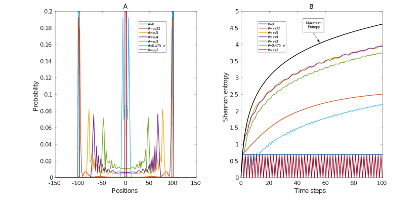
Figure 1: (A) Probability distribution in position space for a discrete-time quantum walker on a line after $T=100$ time steps. Each curve is characterized by a constant value of the parameter $\theta$, while $\xi=\zeta=\pi/2$. (B) Time-evolution of the Shannon entropy, Eq. (10), for the same cases shown in A. The values of $\theta\in\{0,\pi/32,\pi/5,\pi/4,\pi/3,19\pi/40,\pi/2\}$ are color coded.

The time evolution of the system its obtained through the consecutive application of unitary operators, each of them consisting of a coin tossing unitary operator and and conditional shift in position space. The coin operator can be written as a SU(2) matrix

$$\hat{B}(\xi,\theta,\zeta)=\begin{pmatrix}e^{i\xi}\cos\theta&e^{i\zeta}\sin\theta\\ -e^{-i\zeta}\sin\theta&e^{-i\xi}\cos\theta\end{pmatrix},$$ (3)

where $\theta\in[0,\frac{\pi}{2}]$ and $\xi,\zeta\in[0,2\pi]$ chandrashekar08 ; chandrashekar09 . Setting $\xi=\zeta=\frac{\pi}{2}$ we get

$$\hat{B}(\theta)=\begin{pmatrix}\cos\theta&\sin\theta\\ \sin\theta&-\cos\theta\end{pmatrix},$$ (4)

up to a global phase. Note that (4) reduces to the usual Hadamard operator when $\theta=\frac{\pi}{4}$.

The shift operator yields the displacement of the particle in position space conditioned by the internal degree of freedom of the coin, and can be written as

$$\hat{S}=\sum_{x=-\infty}^{\infty}\left(\ket{x+1}\bra{x}\otimes\ket{R}\bra{R}+\ket{x-1}\bra{x}\otimes\ket{L}\bra{L}\right).$$ (5)

In practice, we will consider a finite-dimensional version of Eq. (5), with specific boundary conditions (see Appendix A). Finally, the total unitary evolution operator is given by

$$\ \hat{U}(\xi,\theta,\zeta)=\hat{S}\cdot(\hat{\mathbb{I}}_{p}\otimes\hat{B}(\xi,\theta,\zeta)),$$ (6)

such that

$$\ket{\psi(t+1)}=\hat{U}(\xi,\theta,\zeta)\ket{\psi(t)}.$$ (7)

Since we will consider time-dependent parameters in (3) and (4), the evolution of the system for $T$ time steps will be given by

$$\ket{\psi(t+T)}=\hat{U}_{T}\cdots\hat{U}_{1}\ket{\psi(t)},$$ (8)

where $\hat{U}_{t}=\hat{U}(\xi_{t},\theta_{t},\zeta_{t})$ for time $t$. As our initial state, we will consider a particle localized at $x=0$ and with a coin component of the form

$$\ket{\psi_{S}}\equiv\ket{\psi(0)}=\frac{1}{\sqrt{2}}\ket{0}_{p}\otimes\left(\ket{R}_{c}+i\ket{L}_{c}\right),$$ (9)

leading to a left-right symmetric evolution for $\xi=\zeta=\pi/2$ kendon03 . In this work we will only consider quantum walkers characterized by a sequence $\{\theta_{t}\}_{t=1}^{T}$, with $\xi_{t}=\zeta_{t}=\pi/2$ for all time.

As we can see in Fig. 1A, the typical behavior of the quantum walk using a constant coin-tossing operator is far from being uniform in position space. Instead, the probability distributions show an intrincate interference pattern. The maximal spread is obtained for $\theta=0$, corresponding to $\hat{B}(0)\equiv\hat{\sigma}_{z}$, and the minimal one is found for $\theta=\pi/2$, which corresponds to $\hat{B}(\pi/2)\equiv\hat{\sigma}_{x}$.

The spread of the probability distribution in position space can be characterized using Shannon’s entropy,

$$S=-\sum_{x}P_{x}\log P_{x},$$ (10)

with $P_{x}$ given in Eq. (2). After $t$ time-steps, the maximal value possible for the entropy is given by $S_{\text{max}}(t)=\log(t+1)$. This bound can be understood by noticing that, after $t$ time-steps, the particle can only reach $2t+1$ sites, but only odd (even) positions can be occupied after an odd (even) number of time-steps, in absence of decoherence. Fig. 1B shows the time-evolution of the Shannon’s entropy of a quantum walker for different constant values of $\theta$. Indeed, the maximal bound is never reached, yet for some values of $\theta$ we obtain a logarithmic growth, corresponding to a ballistic spread.

II.1 Optimizing quantum walks

The aim of this work is to obtain the optimal sequence of coin-tossing operators maximizing the spatial spread of the quantum walker along its whole history, up to a certain time-step $T$. We will restrict our search to discrete-time quantum walkers without decoherence and with coin-tossing operators using $\xi_{t}=\zeta_{t}=\pi/2$, i.e.: they will be fully determined by the sequence $\{\theta_{t}\}_{t=1}^{T}$.

For a fixed time-step $t$, a good figure of merit is given by the Shannon entropy of the spatial probability distribution, Eqs. (10) and (2), normalized by the maximal value achievable for that time-step. After $t$ time-steps, the walker can reach a total of $t+1$ sites (not $2t+1$ as one might naively expect, because the walker can only reach even-indexed sites after an even number of steps, and viceversa). Thus, the maximal achievable Shannon entropy after $t$ time-steps is $S_{\text{max}}=\log(t+1)$. Therefore, a reasonable observable to characterize the extent of the spread of the quantum walker after $T$ time-steps is given by

$$F\left(\theta_{0},\cdots,\theta_{T}\right)=1-{1\over T+1}\sum_{t=0}^{T}\frac{S(t)}{\log(t+1)},$$ (11)

where $S(t)$ is the Shannon entropy after $t$ time-steps, given in Eq. (10). This magnitude $F$ reaches its maximum value $F=1$ when the walker is completely localized, while its minimum $F=0$ corresponds to our desired situation, when the spread is maximal along its whole history.

Finding the optimal set of $\{\theta_{t}\}$ which minimizes $F$ is a computationally demanding task. We employ a combination of conjugated gradients method and sampling of initial configurations in order to achieve the global minimum when the target function presents many local minima, as it has been done by other authors santos18 . The number of initial configurations employed was 50 for moderate times, and as high as 200 for the maximal time reached, $T=45$. Our numerical experiments allow us to conjecture that the optimization landscape is rather complex, as it will be discussed in the next section.

III Results

III.1 Different approaches to optimize spread

Our first attempt at obtaining the optimal set of parameters $\{\theta_{t}\}_{t=1}^{T}$ in (4) for an optimal spread is analytical. For $T<4$, we have found the optimal distribution corresponding to the maximal spread, the detailed calculations are provided in Appendix B, here we will only cite the main results. First of all, notice that the spread does not depend on $\theta_{1}$, so this first value is always arbitrary. For the second and third steps, we obtain $\theta_{2}=\arctan(1/\sqrt{2})$ and $\theta_{3}=\frac{\pi}{6}$, respectively. For $T\geq 4$, we have proved that no set of coin-tossing operators will yield this perfect spread. Yet, a numerical evaluation of the $\theta$ sequences yielding an optimal amount of spread is still possible, and the following section is devoted to their characterization.

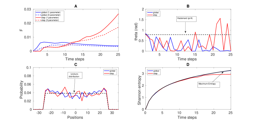
Figure 2: Optimization of the spread, obtained minimizing the value of $F$. We employ two different approaches: global or step-by-step. Moreover, we explore the use of a single coin parameter ($\theta$) or the full set of three parameters. The results are shown up to $T=25$ time steps. (A) Evolution of the minimal $F$ value, as obtained using the different optimization criteria. Note that the actual (and computed) value for the global case is $T=25$; the previous time steps are reconstructed a posteriori. (B) Sequence of $\theta$ parameters that minimize $F$. (C) Probability distribution in position space. (D) Shannon entropy of the probability distribution in position space. Note that the global case overlaps with the maximum entropy case.

For a given number $T$ of time steps, there are a few different approaches to the optimization of the set of $\theta$ parameters.

• We may minimize a single global value of $F$ spanning time-steps 1 to $T$, i.e. obtain the whole set of $\theta$ parameters in a single optimization procedure.

• Alternatively, we can operate through a step-by-step minimization: once the sequence $\theta_{1}$ to $\theta_{t}$ is optimized, we obtain the optimal value of $\theta_{t+1}$, and iterate up to $t=T$.

• Finally, we can optimize only the value of the final spread, after $T$ time-steps, disregarding the intermediate stages. This procedure always results in an optimal spread. We will not discuss this approach further in the main text, and leave the details for Appendix C.

In Fig. 2 we compare the first two approaches. The step-by-step method achieves a better optimization for short times, but the value of $F$ (which measures our failure to obtain perfect spread) increases fast between $T=10$ and $T=15$, and for large times the global procedure is considerably better (Fig. 2A). Note that the global approach only provides a single value of $F$, corresponding to the final time step; but in the figure we provide an a posteriori reconstruction of the $F$ values for all times. The sequence of $\theta$ parameters is different for each approach, with some unexpected differences. For example, all $\theta$ values are below $\frac{\pi}{4}$ for the global approach, while they can reach values above that threshold for the step-by-step procedure, specifically near the time where the technique starts to fail (Fig. 2B). We can see the final probability distribution for the two approaches and its difference with a perfectly uniform one in Fig. 2C. Finally, in Fig. 2D we can observe the evolution of the Shannon entropy of the probability distribution, compared to its maximal possible value. Notice how the globally obtained entropy remains close this maximum possible value, while the step-by-step entropy deviates from it. Henceforth, given its higher precision, we will make use of the global approach in the rest of this work.

The minimal value of $F$ obtained using all three parameters of the coin-tossing operator ($\xi$, $\theta$ and $\zeta$ in Eq. (3)) will be always equal or lower than the value obtained using only the parameter $\theta$ and $\xi=\zeta=\pi/2$ (i.e., using Eq. (4)). Interestingly, the difference gets smaller with time when we follow the global optimization approach, as we can see in Fig. 2A. Similar results have been reported when analyzing entanglement properties vieira14 . Henceforth we will consider only the coin operator (4) with one parameter.

III.2 Characterization of the Optimal Sequences

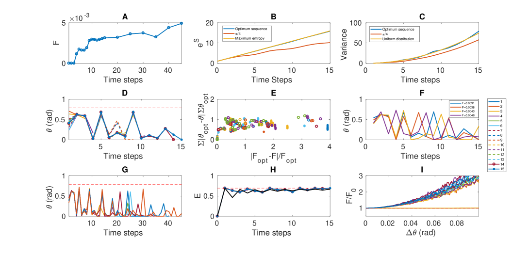
Figure 3: Optimized sequences of the $\theta$ parameters for $T=1,\cdots,15$. (A) Minimal $F$ values for different $T$ under global optimization. (B) Exponential of the Shannon entropy ($S$) of the probability distribution in position space and (C) variance for the optimum sequence for $T=15$, compared to the results using the Hadamard coin operator ($\theta=\frac{\pi}{4}$). Note that the Shannon entropy for the optimum case overlaps with the maximum entropy situation. (D) Optimized $\theta$ parameters for $T=1$ up to $T=15$. The horizontal dashed red line corresponds to $\frac{\pi}{4}$ (Hadamard). (E) Differences of local minima with respect to the optimum case computed as the difference in the $F$ value and the $\theta$ parameter. Each symbol corresponds to optimization for different time steps ($T=1..15$). (F) Four lowest local minima for $T=15$. (G) Optimized sequences of $\theta$ parameters for $T=5,10,15,20,25,30,35,40,45$. The horizontal dashed red line corresponds to $\frac{\pi}{4}$ (Hadamard). (H) Time evolution of the von Neumman entropy of the reduced density matrix as a measure of entanglement for the optimized sequences of $\theta$ parameters for $T=1$ up to $T=15$. The black line corresponds to the mean value of 1000 simulations with random $\theta$ parameters. The horizontal red dashed line corresponds to the situation of maximum entanglement $\log(2)$. (I) Stability of the optimized sequences of $\theta$ parameters against increasing perturbations (noise) of the $\theta$ value (see text). For the case $T=1$ there is no change; and for $T=2,3$ the changes are not appreciable.

Figure 3A shows how the minimal $F$ values increase as the final time $T$ increases. As it was expected, the spread is perfect for $T\leq 3$. As shown before, the Shannon entropy for the optimum sequence ($T=15$) is very close to the maximum value when compared to the usual Hadamard case (Fig. 3B). Let us remind the reader that the variance in position space is defined by $\sigma^{2}=\langle x^{2}(t)\rangle-\langle x(t)\rangle^{2}$. Thus, considering that for even (odd) time steps only the even (odd) sites are occupied and that the probability distribution in position space is uniform, the variance of an idealized uniform quantum walk takes the form

$$\begin{split}\sigma_{T}^{2}&=\frac{2}{T_{\textrm{even}}+1}\sum_{0}^{T_{\textrm{even}}/2}(2T_{\textrm{even}})^{2}\\ &=\frac{2}{T_{\textrm{odd}}+1}\sum_{0}^{(T_{\textrm{odd}}-1)/2}(2T_{\textrm{odd}}+1)^{2}\\ &=\frac{1}{3}\frac{T(T^{2}+3T+2)}{T+1}.\end{split}$$ (12)

The evolution of the variance for the optimal sequence for $T=15$ is, indeed, very similar to our analytical expression (12), as we can check in Fig. 3C. The optimal sequences of $\theta$ parameters are depicted in Fig. 3D. Unfortunately, they do not present a regular pattern which can help us predict their evolution for larger time spans. Yet, optimal sequences obtained for low values of $T$ are very similar among themselves, but differences become significant for optimal sequences corresponding to longer times, as we can check in Fig. 3G. Nonetheless, there are some manifest patterns in the optimal sequences, such as an alternation between values close to $\theta=\frac{\pi}{4}$ and $\theta=0$, with increasing periods. We will discuss this pattern later in this section. Notice that all $\theta$ parameters are always below $\theta_{c}=\frac{\pi}{4}$.

During the optimization procedure we obtain on occasion local minima of the target function $F$ which do not correspond to the global minimum, $F_{\textrm{opt}}$. In Fig. 3E we have considered these local minima. For each local solution we provide a point in the plot, where the abscissa is given by $|F-F_{\textrm{opt}}|$ and the ordinate provides the difference in the $\theta$ values, defined as

$$\Delta[\{\theta_{i}\}]\equiv{\sum_{i=1}^{T}|\theta_{i}^{\textrm{opt}}-\theta_{i}|\over(\sum_{i=1}^{T}\theta_{i}^{\textrm{opt}})}.$$ (13)

The resulting plot provides the image of a complex landscape, with a great variety of local minima, typical of glassy systems, which might be related to replica symmetry breaking ueda14 ; itoi17 . As an illustration, Fig. 3F depicts the optimal sequence for $T=15$ along with the three lowest-$F$ local minima.

Since we are neglecting decoherence, the complete system state (particle and coin) remains pure throughout time evolution. Thus, we can make use of the von Neumann entropy of the reduced density matrices as a measure of the entanglement between particle and coin,

$$E(t)=-\Tr[\rho_{1}(t)\ln\rho_{1}(t)]=-\Tr[\rho_{2}(t)\ln\rho_{2}(t)],$$ (14)

where $\rho_{1,2}(t)=Tr_{2,1}\rho(t)$ are the reduced density matrices of the position and coin degrees of freedom, respectively, and $\rho(t)=\ket{\psi(t)}\bra{\psi(t)}$. We compare the entanglement of the optimized sequences for different time steps with the the case of random evolution of the $\theta$ parameters in Fig. 3H. As we can readily see, the entanglement of the optimized sequences tends to its maximum value, as in the random case, but slightly faster.

In order to test the robustness of the optimized $\theta$ sequences, we have introduced an increasing amount of noise in the parameters, $\theta_{i}\to\theta_{i}+\Delta\theta\cdot\eta_{i}$, where the $\eta_{i}$ are i.i.d. Gaussian random variables of zero average and unit variance. Let $F_{0}$ be the optimal value for $F$ for the maximal $T$. For all values of the noise amplitude, $\Delta\theta$, we evaluate $F$ for $N_{s}=10^{3}$ different random perturbations of the optimal sequence, and the quotient $F/F_{0}$ is plotted in Fig. 3I. For consistency, values of $\theta_{i}$ that leave the range $[0,\pi/2]$ are automatically set to the closest extreme of the interval. As expected, we observe a smooth increase of the optimal value of $F$.

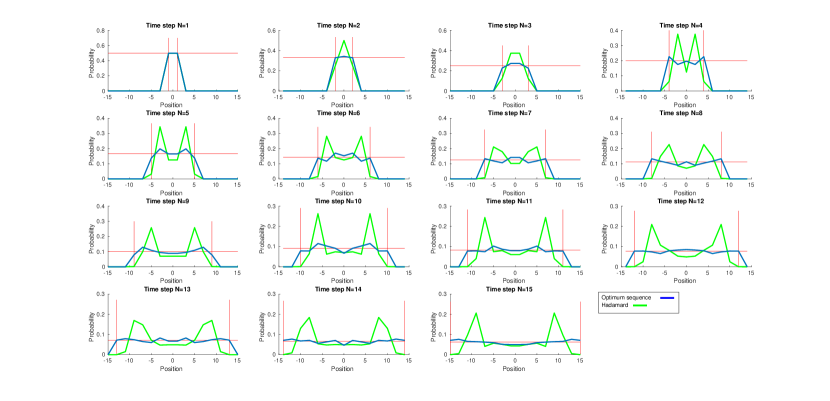
Figure 4: Evolution of the probability distribution in position space, $P(x,t)=|\langle x|\psi_{L}(t)\rangle|^{2}+|\langle x|\psi_{R}(t)\rangle|^{2}$ for the optimized set of $\theta$ parameters (blue), and the Hadamard coin operator (green) for $T=15$ time steps. The vertical red lines represent the maximum possible extension for a quantum walk and the horizontal line represents the probability value corresponding to a perfectly uniform distribution.

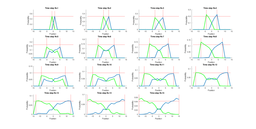
Figure 5: Evolution of the probability distribution in position space for $P_{R}(x,t)=|\langle x|\psi_{R}(t)\rangle|^{2}$ (blue) and $P_{L}(x,t)=|\langle x|\psi_{L}(t)\rangle|^{2}$ (green) for the optimized set of $\theta$ parameters for $N=15$ time steps. The vertical red lines represent the maximum possible extension for a quantum walk and the horizontal line represent the probability value corresponding to a perfectly uniform distribution.

Let us stress that we require uniformity of the probability in position space throughout the $T$ time-steps, not just the last one. Figure 4 illustrates this fact comparing the evolution of the optimum sequence for $T=15$ with the Hadamard coin operator for each time step. As we can readily see, the spreading of the optimum sequence is always larger than in the Hadamard case, and the probability distribution much more flat. Note that, even though it is possible to achieve a perfectly uniform distribution up to $T=3$, in this case there is some deviation because the optimization target is set to all times up to $T=15$.

IV Understanding the Optimal Sequences

The optimal values of $\theta_{i}$ for different final times $T$ are plotted in Fig. 3G. Although they do not follow a fixed pattern, the optimal sequences present relevant features, such as a non-periodic alternation of values $\theta\approx 0$ (coin-tossing operator close to $\sigma_{z}$) and $\theta\approx\pi/4$ (close to $\sigma_{x}$). In intuitive terms, the values of $\theta\approx 0$ split the wavefunction, making the left and right parts advance separately in each direction, while values close to $\theta\approx\pi/4$ combine both components again. Thus, the optimal sequences are composed of a certain alternation of both types of quantum operators: advance and mixture.

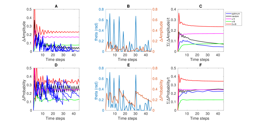
Figure 6: (A) Evolution of the amplitude overlap between $\ket{\psi_{R}(t)}$ and $\ket{\psi_{L}(t)}$ for the optimized sequences $T=1\cdots 15,20,25,30,35,40,45$. (B) Evolution of the amplitude overlap and the $\theta$ parameters for the optimum sequence of $T=45$. (C) Evolution of the sum of the normalized amplitude overlapping for different optimizations ($T=1\cdots 15,20,25,30,35,40,45$). (D) Evolution of the probability overlapping between $\ket{\psi_{R}(t)}$ and $\ket{\psi_{L}(t)}$ for the optimized sequences $T=1..15,20,25,30,35,40,45$. (E) Evolution of the probability overlapping and the $\theta$ parameters for the optimum sequence of $T=45$. (F) Evolution of the sum of the normalized probability overlapping for different optimizations ($T=1...15,20,25,30,35,40,45$). The results from the random sequences were obtained as the mean value for 500 random simulations.

Following Eq. (1) we can write the state of the system $\ket{\psi(t)}$ as

$$\ket{\psi(t)}=\ket{\psi_{L}(t)}\ket{L}+\ket{\psi_{R}(t)}\ket{R}.$$ (15)

where $\ket{\psi_{\{L,R\}}}=\sum_{x}\psi_{x,\{L,R\}}\ket{x}$ need not be normalized orthey17 . This allows us to decompose the spatial probability distribution $P(x,t)=P_{L}(x,t)+P_{R}(x,t)$, where $P_{L}(x,t)=|\langle x|\psi_{L}(t)\rangle|^{2}$ and $P_{R}(x,t)=|\langle x|\psi_{R}(t)\rangle|^{2}$. Fig. 5 shows the time evolution of both probability distributions. Notice their left-right symmetry: $P_{L}(x,t)=P_{R}(-x,t)$. Moreover, we can also consider the overlap (or fidelity) between the two wavefunctions:

$$\Delta_{A}(t)\equiv\absolutevalue{\innerproduct{\psi_{R}(t)}{\psi_{L}(t)}}^{2},$$ (16)

whose behavior is shown in Fig. 6A. We can observe that this overlap decays towards zero for all values of $T$, faster than for all other quantum walks, including (an average over) random values. In Fig. 6B we can see both the overlap and the optimal $\theta_{i}$ values for $T=45$, which present little correlation. Indeed, we can also define an average degree of overlap along an optimized trajectory,

$$\Delta_{A}^{\textrm{norm}}=\frac{1}{T}\sum_{t=1}^{T}\Delta_{t}.$$ (17)

We show its behavior in Figure 6C. The conclusions are manifestly disappointing.

Luckily, a slightly different magnitude presents a much more clarifying behavior. Let us define the probability overlap as the area under the minimum:

$$\Delta_{P}(t)=\sum_{x}\min(P_{L}(x,t),P_{R}(x,t)),$$ (18)

which is one if both probability distributions coincide, and zero if their supports do not intersect. Fig. 6D presents the time-evolution for the same cases considered in Fig. 6A. In this case we can observe a sawtooth behavior in the values of the probability overlap for the optimal sequence, oscillating around a finite value. Fig. 6E shows that quick increases in the probability overlap are caused for large values of $\theta_{i}\approx\pi/4$, while small values ($\approx 0$) allow it to decay linearly. The competition between these pulls and pushes resembles a tug-of-war which gives rise to the desired optimal spread. Fig. 6F plots the time-averaged values of the probability overlap, where we can see that they reach a limit value which is different from zero. This limit value can be roughly estimated by considering that the probability distributions $P_{L}(x,t)$ and $P_{R}(x,t)$ are approximately linear for long time steps, which can be verified in the last panels of Fig. 5. In this way, the probability overlap is the area of an isosceles triangle with altitude $\frac{1}{2(T+1)}$ and base $N=2T+1$, so for discrete positions and odd time steps (only odd positions are occupied) we have

$$\begin{split}A=&\frac{4}{N(N+2)}\sum_{n=1}^{N/2}n\\ =&\frac{4}{N(N+2)}\sum_{n=0}^{(N-2)/4}(2n+1)\underset{N\rightarrow\infty}{=}\frac{1}{4},\end{split}$$ (19)

where we have taken the limit $N\rightarrow\infty$ to obtain our estimate for the long term probability overlap. Yet, oscillations are expected for a large time range. Interestingly, the time-averaged probability overlaps depicted in Fig. 6F for optimal sequeces are slightly below the (averaged) values obtained for random sequences, which also tend to a finite value in the long term.

Summarizing, the results obtained so far suggest that the pattern of optimal $\theta$ parameters is, indeed, complex. Their most salient feature is a strong alternation of values close to $0$ or to $\pi/4$, with increasingly long periods. Yet, we show in Appendix D) that, based on scaling arguments, we can conjecture that the optimal $\theta$ values will decay in time like $\propto\arcsin\left(\frac{1}{t}\right)$.

IV.1 Spectral Properties of the Optimal Evolution Operator

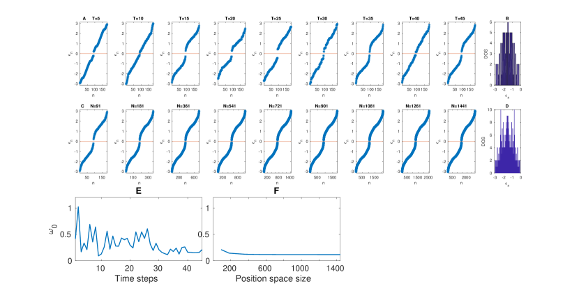
Figure 7: (A) Spectrum $\epsilon_{n}=i\log(\lambda_{n})$ where $\lambda_{n}$ are the eigenvalues of the unitary operator $\hat{U}(N)$ for different optimization with increasing time steps values. (B) Density of states of the lowest band of the spectrum of $T=45$. (C) Spectrum $\epsilon_{n}=i\log(\lambda_{n})$ where $\lambda_{n}$ are the eigenvalues of the unitary operator $\hat{U}(45)$ with increasing positions space size. (D) Density of states of the lowest band of the spectrum for the positions space size of $N=1441$. (E) Time evolution of the miminum positive value of the spectrum of $\hat{U}(45)$ where we have considered that $\hat{U}(45)=\hat{U}_{45}...\hat{U}_{1}$. (F) Evolution of the minimum positive value of the spectrum of $\hat{U}_{45}$ with increasing positions space size.

In this subsection we discuss the energy spectrum of the optimum evolution operator. Since the evolution is explicitly time-dependent, the system is non-autonomous and, hence, we cannot define an energy spectrum. Yet, we can consider the quasi-energy spectrum, which can be defined as $\epsilon_{n}=i\log(\lambda_{n})$ where $\lambda_{n}$ are the eigenvalues of the unitary operator $\hat{U}_{N}$ gullo17 ; buarque19 . It is interesting to consider the asymptotic properties of the system for which it is necessary to study the spectrum of the total evolution operator for a time step $t$ such $\hat{U}(t)=\hat{U}_{t}\hat{U}_{t-1}...\hat{U}_{2}\hat{U}_{1}$, where $t\gg 1$. Due to the computational cost of optimizing quantum walks for large time lapses, we are limited to $T=50$. It has been shown, at least for certain aperiodic sequences as well as for simple periodic ones, that after few steps ($t\sim 30$) the spectrum of the total evolution operator does not change appreciably gullo17 .

We show the results in Fig. 7. First, we obtain the spectra for different optimizations corresponding to increasing time steps (Fig. 7A,B), where the size of the position space is the minimum possible to avoid boundaries (i.e. $2T+1$). As we are considering finite-dimension Hilbert spaces, we obtain discrete point spectra, where the appearence of a gap around $\epsilon_{k}=0$ can be appreciated. It is interesting to compare this quasi-energy spectrum with the asymptotic spectra of certain aperiodic and periodic sequences, where such a gap does not appear gullo17 . Let us consider the spectrum of $\hat{U}(T=45)$ for different system sizes, where we can see that the gap is maintained in Fig. 7C,D.

We can see also consider the time evolution of the quasi-spectral gap of $\hat{U}(t)$, fixing $T=45$, as it is shown in Fig. 7E. Notice that, despite the fluctuations, it seems to tend to a finite value, although larger time lapses would be required in order to confirm this tendency. The quasi-spectral gap does not possess a relevant dependence on the system size $N$, as we can see in Fig. 7F.

The energy spectrum for constant $\theta$ values can be interpreted as a dispersion relation $E(k)$ buarque19 . As the quasi-energy spectrum remains unchanged for long enough times (Fig. 7A, (gullo17, )) it is natural also to interpret it as a dispersion relation. Furthermore, for constant values of $\theta$ we can obtain an analogue of the Klein-Gordon equation for $\psi_{R}$ and $\psi_{L}$, where the mass is given by chandra10

$$M=\sqrt{2(\sec{(\theta)}-1)\over\cos{(\theta)}},$$ (20)

This implies that for $\theta=0$ the quantum walker is equivalent to a massless particle, presenting a gapless linear spectrum and non-zero group velocity. On the other hand, for increasing values of $\theta$ there appears an increasing gap (and therefore an increasing mass) buarque19 . For $\theta=\pi/2$ we have an particle with infinite mass and zero group velocity (its spectrum is flat and gapped). Moreover, it has been shown that periodic and some aperiodic sequences yield gapless spectra, which can be both linear and non linear, respectively gullo17 . They can be understood to represent massless particles of constant and variable group velocity, respectively.

Our optimal sequences present a non linear gapped spectrum, similar to the random sequences, so they can be understood as the evolution of a massive particle with variable group velocity. The reason can be described as follows. In order to explore space efficiently, the quantum walker should be able to reach the maximal possible spread with a finite probability, but it should also reach all other possible sites, with a similar probability. Thus, it should evolve with different propagation velocities, ranging from the maximal velocity, corresponding to $\theta=0$ and the minimal one, corresponding to $\theta=\pi/2$. The group velocities are evaluated from

$$v_{g}(k)={dE(k)\over dk},$$ (21)

which covers a broad range, as we can see from Fig.7.

IV.2 Survival probability

In order to understand the asymptotic dynamics of the system (and study its behavior in relation with the spectral properties) we introduce the survival probability, which it is defined via its amplitude

$$\nu(t)=\innerproduct{\psi(0)}{\psi(t)},$$ (22)

where $\ket{\psi(t)}=\hat{U}(t)\ket{\psi(0)}$. Physically, it describes the probability of finding the state in the time step $t$ in the initial state, that in our case is $\ket{\psi(0)}=\frac{1}{\sqrt{2}}\ket{0}(\ket{R}+i\ket{L})$. Note that it is not strictly the probability of finding the evolved state in the initial position, but in the initial state. The survival amplitude is also directly related to the Fourier transform of the spectral measure of the evolution operator last96 so that

$$\absolutevalue{\nu(t)}^{2}=\absolutevalue{\int_{\sigma}{}d\mu_{0}(\epsilon)e^{-i\epsilon t}}^{2},$$ (23)

where $\mu_{0}$ is the measure induced by the initial state. We have the important result that the Fourier transform of the survival probability is the measure itself.

We will also obtain the time average of the survival probability (Cesáro average) defined as

$$\ \langle\absolutevalue{\nu}^{2}\rangle_{T}=\frac{1}{T}\sum_{t=1}^{T}\absolutevalue{\nu(t)}^{2}.$$ (24)

We can obtain the maximum survival probability and its Cesáro average for an idealized uniform distribution in position space given as

$$\ \nu(t)^{uni} =\frac{1}{\sqrt{t+1}},$$ (25)

$$\ \langle\absolutevalue{\nu}^{2}\rangle_{T}^{uni} =\frac{1}{T}\sum_{t=1}^{T}\frac{1}{t+1}.$$ (26)

We represent in Figure 8A the absolute value of the survival probability, $|\nu(t)|$, computed with (25), for different quantum walks, as in the previous sections. Concretely, we use optimized sequences for several values of $T$, (averaged) values for random sequences and the $\theta_{i}=\pi/4$ quantum walk. Moreover, we also compare to the uniform wavefunction, which is given by

$$\ket{\psi_{U}(T)}={1\over\sqrt{2}}\sum_{x=-T}^{T}\left(\ket{x,L}+\ket{x,R}\right).$$ (27)

The right panel, 8B, shows the Cesáro averaged values. Clearly, random sequences provide the largest value (in average) for the survival probability, while optimal and uniform values stay between the random and the Hadamard cases. Indeed, the uniform and the optimal values remain similar for all times. The behaviour of the Cesáro averages is quite similar.

There are important connections between the survival probability and its Cesáro average and the spectral properties of the system. The spectral measure can be splitted into three parts: pure point, singular continuous and absolute continuous fillman17 . Pure point spectrum is usual for disorderd systems when the $\theta$ is randomly distributed while the absolutely continuous spectrum is related to highly structured systems, such as periodic sequences of quantum coins fillman17 . The singular continuous spectrum appears in between, for example when there is aperiodicity gullo17 . Heuristically, we can assert that the amount of order in the coin parameters is directly related to how continuous the spectral measure is.

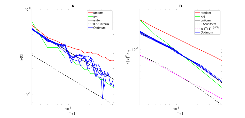
Figure 8: (A) Absolute value of the survival amplitude $\absolutevalue{\nu(t)}$ for different optimum sequences obtained for differents time steps ($T=1...15,20,25,30,35,40,45$). (B) Corresponding Cesáro averages of $\absolutevalue{\nu(t)}^{2}$. In both cases, the black line corresponds to the maximum values of a perfectly uniform distribution ((25) in A and (26) in B) and the red line to the mean value of $N_{s}=500$ random simulations. We have added the uniform distribution with a factor of 0.5 (black dashed line) for a better understanding due to the complete overlapping of the optimum sequences (blue lines) with the uniform distribution (black line). For the Cesáro averages we have added a $1/\sqrt{T+1}$ function (magenta dashed line) for comparative purposes; the uniform distribution corresponds to (26).

For long times, we use the fact that the survival amplitude is the Fourier transform of the measure (23), so we can extract information of the spectrum studying the long-term behaviour of (22) and (24). Specifically, we use the conditions derived from Wiener’s lemma queffelec10 and the theorem of Ruelle, Amrein-Georgescu and Enss (RAGE) (last96 ; fillman17 for the discrete-time version). Indeed, the following conditions

$$\lim_{t\to\infty}\langle\absolutevalue{\nu}^{2}\rangle_{T}=0,$$ (28)

$$\lim_{t\to\infty}\absolutevalue{\nu(t)}=0,$$ (29)

imply that the spectrum of the evolution operator will be absolutely continuous. The first one, Eq. (28), guarantees that the spectrum lacks a pure point part and the second one, Eq. (29), ensures that the spectrum is absolutely continuous. Despite our computational limitations regarding the maximal time-step, we can extract relevant information from the time-evolution of the idealized uniform system, since we know that the survival probability and Cesáro averages are similar to those of the optimized sequences. This implies that, since both conditions (28) and (29) are met, the spectrum of the uniform quantum walk in the limit $t\rightarrow\infty$ is absolutely continuous. It is interesting to note that the aperiodic sequences commented above induce a singular continuous energy spectrum since (29) is not met, but the periodic sequences behave similarly as the optimum sequence since both conditions are met yielding absolutely continuous energy spectra gullo17 .

As noted in fillman17 , using the discrete-time version of the RAGE theorem we can relate the different spectral types commented above with the localization/spreading behavior of the wavefunction:

• Pure point: most of the wavepacket never leaves a given bounded region, so the wavefunction will remain localized.

• Singular continuous: upon time-averaging, the wavepacket will eventually leave any bounded region, but this could not be true of all walks.

• Absolutely continuous: most of the wavepacket will eventually leave any bounded region. In one dimension the spread will be ballistic upon time averaging and, without averaging, for some specific quantum walks.

Asymptotically, the behaviour of the optimum sequence is expected to be similar to that studied for finite times: the wavepacket spreads ballistically leaving any bounded region. Curiously, this is also the behaviour of periodic sequences: the optimal sequence seems not be periodic, but asymptotically behaves as a highly ordered periodic sequence. Contrarily, the aperiodic sequences can show anomalous transport, i.e. the wavepacket leaves any bounded region with sub-ballistic speed. Furthermore, we have the expected analytical expression for the survival probability (25) and the Cesáro average (26) of the optimum sequence, providing the exact exponent of the power-law decay; for aperiodic sequences the maximum value of this exponent is $\sim 0.8$ gullo17 . It is also interesting to note that random sequences do not seem to fulfill conditions Eq. (28) and Eq. (29), implying that they present a pure point spectrum yielding a localized wavefunction.

V Conclusions

In this article we have provided a protocol to build a time-dependent quantum walk which provides optimal spatial spread, i.e.: for which the spatial distribution is (nearly) maximal for all time steps. We have restricted ourselves to coin-tossing operators with a single parameter, $\theta$, because the inclusion of all three Euler angles does not improve the results substantially. The optimal sequences depend on the maximal time considered, $T$, and present complex structures. Yet, some patterns arise. First of all, most values are close to either $\theta=0$ or $\theta=\pi/4$. The first values tend to stretch the left and right parts of the wavefunction. The second ones tend to appear when the probability overlap has fallen below a certain threshold, and allow the wavefunction to combine again. Even though finding the optimal sequences can be a complicated optimization problem, a crude estimate can be obtained.

We have considered the long-term dynamics associated with these optimal quantum walk, regarding the survival probability (the fidelity with the initial state) and the spectrum of the evolution operator. The observed behavior leads to conjecture that the spectrum is absolutely continuous, a behaviour typical of highly ordered sequences as the periodic ones.

Regarding lines of future work, we are interested in quasi-optimal sequences, alternating $\theta=0$ and $\theta=\pi/4$ values in a regular (although non-trivial) pattern which will give rise to a quasi-optimal spread. Indeed, these quasi-optimal sequences will be much easier to obtain in the laboratory. Moreover, we intend to obtain the corresponding values in $>1D$ and disordered lattices. It is very relevant to consider the search capabilities of these optimized quantum walks, which will be substantially improved over time-independent or random quantum walks.

VI Acknowledgements

We would like to acknowledge Silvia N. Santalla and Germán Sierra for useful discussions. This work has been partially funded by the Spanish Government and the European Union through grant QUITEMAD-CM P2018/TCS-4342.

Appendix A Boundary conditions for the evolution operator

As mentioned in section II, the unitary evolution operator (7) is defined on an infinite dimensional Hilbert space associated to all possible positions. For practical purposes, (i.e. numerical analysis) we need to consider a finite dimensional positions space, but this may turn non-unitary both the shift operator (5) and, therefore, the evolution operator (7). We solve this issue, formally, by defining cyclic boundary conditions in such a way that the shift operator is defined by $\hat{S}=\hat{S}_{c}+\hat{S}_{b}$ where

$$\begin{split}\hat{S}_{c}=&\left(\sum_{x=1}^{N-1}\ket{x+1}\bra{x}\right)\otimes\ket{R}\bra{R}+\\ &\quad+\left(\sum_{x=2}^{N}\ket{x-1}\bra{x}\right)\otimes\ket{L}\bra{L},\end{split}$$ (30)

$$\hat{S}_{b}=\ket{1}\bra{N}\otimes\ket{R}\bra{R}+\ket{N}\bra{1}\otimes\ket{L}\bra{L},$$ (31)

where $N$ is the finite size of the position space. We always consider that the particle starts in the middle of the positions space (i.e. $x=0$), so if we set the size of the positions space as $N=2T+1$, where $T$ is the number of time steps, the particle never actually experiences the boundary conditions. Nevertheless, when analyzing spectral properties of the evolution operator the boundary conditions are evaluated.

Appendix B QRW fails to be uniformly distributed in space for $N=4$

We now show that a QRW using a time-dependent coin operator of the form (4) can not be uniformly distributed in positions space when considering a symmetric initial state (9).

Considering that the probability for the particle to be at $x=i$ at time-step $t$ is given by

$$Pr_{i}(t)=\Tr[(\ket{i}\bra{i}\otimes\hat{\mathbb{I}}_{p})\cdot\hat{\rho}(t)],$$ (32)

we have that, for all $t$,

$$\sum_{x=-t}^{t}\Tr[\left(\ket{x}\bra{x}\otimes\hat{\mathbb{I}}_{p}\right)\cdot\hat{\rho}(t)]=1,$$ (33)

where $\hat{\rho}(t)=\ket{\psi(t)}\bra{\psi(t)}$ is the density operator at time step $t$, and

$$\hat{\rho}(t)=\hat{U}_{t}\cdots\hat{U}_{1}\hat{\rho}(0)\hat{U}_{1}^{{\dagger}}...\hat{U}_{t}^{{\dagger}}.$$ (34)

This is valid for any initial state $\hat{\rho}(0)$, but from here we will consider that $\hat{\rho}(0)=\ket{\psi_{S}}\bra{\psi_{S}}$, where $\ket{\psi}_{S}$ is the symmetric state (9). Note that, due to the cyclic properties of the trace, for an uniform probability distribution in positions space we should have

$$\ \Tr[\hat{P}(t)\cdot\hat{\rho}(0)]=\frac{1}{t+1}$$ (35)

where $\hat{P}(t)=\hat{U}_{1}^{{\dagger}}...\hat{U}_{t}^{{\dagger}}\left(\ket{0}\bra{0}\otimes\hat{\mathbb{I}}_{c}\right)\hat{U}_{t}...\hat{U}_{1}$ for even time steps and $\hat{P}(t)=\hat{U}_{1}^{{\dagger}}...\hat{U}_{t}^{{\dagger}}\left(\ket{1}\bra{1}\otimes\hat{\mathbb{I}}_{c}\right)\hat{U}_{t}...\hat{U}_{1}$ for odd time steps. Thus, it would be necessary only to evaluate the operator $\hat{P}(t)$.

Let us prove it directly by evaluating (33) for $t=1,2,3,4$ and substituting the solutions sequentially, searching for the values of $\{\theta_{i}\}$ that will make all the spatial probabilities equal.

• $t=1$

  $$\ Pr_{x=-1}=Pr_{x=1}=\frac{1}{2},$$ (36)

  and there is no dependence on $\theta_{1}$. Thus, $\theta_{1}$ can take any value in $[0,\frac{\pi}{2}]$.

• $t=2$

  $$\begin{split}\ Pr_{x=-2}&=Pr_{x=2}=\frac{1}{2}\cos^{2}(\theta_{2}),\\ \ Pr_{x=0}&=\sin^{2}(\theta_{2}),\end{split}$$ (37)

  whose solution is $\theta_{2}=\arctan(\frac{1}{\sqrt{2}})$.

• $t=3$

  $$\begin{split}\ Pr_{x=-3}=Pr_{x=3}&=\frac{1}{3}\cos^{2}(\theta_{3}),\\ \ Pr_{x=-1}=Pr_{x=1}&=\frac{1}{2}-\frac{1}{3}\cos^{2}(\theta_{3}),\end{split}$$ (38)

  whose solution is $\theta_{3}=\frac{\pi}{6}$.

• $t=4$

  $$\begin{split}\ Pr_{x=-4}&=Pr_{x=4}=\frac{1}{4}\cos^{2}(\theta_{4}),\\ \ Pr_{x=-2}&=Pr_{x=2}=\frac{1}{3}-\frac{1}{6}\cos^{2}(\theta_{4})+\frac{\sqrt{2}\cos(\theta_{4})\sin(\theta_{4})}{12},\\ \ Pr_{x=0}&=\frac{1}{3}-\frac{1}{6}\cos^{2}(\theta_{4})-\frac{\sqrt{2}\cos(\theta_{4})\sin(\theta_{4})}{12},\end{split}$$ (39)

  and, in this case, the system is incompatible.

Appendix C Optimization for the final step

As we did in Figure 3, let us perform the optimization process imposing the only condition that the probability distribution be uniform in the last step, where instead of using Eq. (11) we define a new function

$$F^{\prime}(\theta_{0},...,\theta_{T})=1-\frac{S(\theta_{0},...,\theta_{T})}{S_{max}^{T}},$$ (40)

where $S$ is the Shannon entropy. Function (40) is normalized so that $F=1$ for a completely localized particle, and $F=0$ for a completely uniform distributed particle in the last time step. The results are shown in Fig. 9. As expected, the values for $F$ are considerably lower (seven orders of magnitude) and the Shannon entropy only matches the maximum value at the last time step. Regarding the $\theta$ values, they exceed $\frac{\pi}{4}$ and do not approach zero. Moreover, they do not show any recognizable pattern. As expected, the robustness is high and the procedure tolerates higher noise in the parameters. The optimization in the last step could be useful, for example, for preparing the system in a uniform distribution for a given time step.

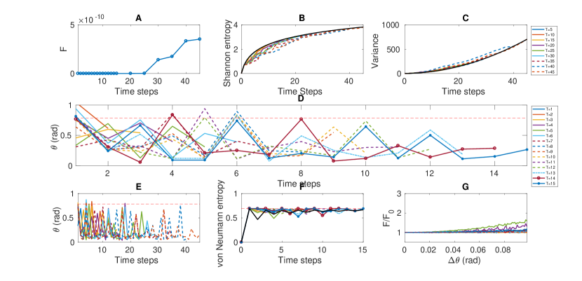
Figure 9: Optimized sequences of the $\theta$ sequences for $T=1...15,20,25,30,35,40,45$ for the last-time step optimization, Eq. (40). (A) Evolution of the $F^{\prime}$ value for different time steps optimizations. (B) Exponential of the Shannon entropy of the probability distribution in positions space and (C) variance for the optimum sequence for $T=5,10,15,20,25,30,35,40,45$. (D) Optimized sequences of $\theta$ parameters for $T=1$ up to $T=15$. The horizontal dashed red line corresponds to $\frac{\pi}{4}$ (Hadamard). (E) Optimized sequences of $\theta$ parameters for $T=1..15,20,25,30,30,35,40,45$. The horizontal dashed red line corresponds to $\frac{\pi}{4}$ (Hadamard). (F) Time evolution of the von Neumman Entropy of the reduced density matrix as a measure of entanglement for the optimized sequences of $\theta$ parameters for $T=1$ to $T=15$. The black line corresponds to the mean value of 1000 simulations with random $\theta$ parameters. The horizontal red dashed line corresponds to the situation of maximum entanglement $\log(2)$. (G) Stability of the optimized sequences of $\theta$ parameters against increasing perturbations (noise) of the $\theta$ value (see text).

Appendix D Optimal parameters in the long time limit

Let us estimate the behavior of the optimal $\theta$ values for long times. Lets consider the positions $x=+1$ and $x=-1$ for an odd time step $t$ and $x=0$ for even time steps $t+1$ so that

$$\ket{\psi_{-1}(t)}=\ket{-1}\left(r_{-1}\ket{\uparrow}+l_{-1}\ket{\downarrow}\right),$$ (41)

$$\ket{\psi_{1}(t)}=\ket{1}\left(r_{1}\ket{\uparrow}+l_{1}\ket{\downarrow}\right),$$ (42)

$$\ket{\psi_{0}(t+1)}=\ket{1}\left(r_{0}\ket{\uparrow}+l_{0}\ket{\downarrow}\right),$$ (43)

where $r_{-1}$, $r_{1}$, $l_{-1}$, $l_{1}\in\mathbb{C}$ are probability amplitudes (where we have omitted the time dependence), and $r_{0}$ and $l_{0}$ are given by

$$r_{0}=r_{-1}\cos\theta_{t}+l_{-1}\sin\theta_{t},$$ (44)

$$l_{0}=r_{1}\sin\theta_{t}-l_{1}\cos\theta_{t}.$$ (45)

Due to the uniform probability distribution restriction and that $|\psi_{R}(t)|^{2}$ and $|\psi_{L}(t)|^{2}$ are symmetric with respect to $x=0$, the following conditions are fulfilled

$$|r_{-1}|^{2}+|l_{-1}|^{2}=|r_{1}|^{2}+|l_{1}|^{2}=\frac{1}{t+1},$$ (46)

$$|r_{1}|^{2}=|l_{-1}|^{2},$$ (47)

$$|r_{-1}|^{2}=|l_{1}|^{2},$$ (48)

$$|r_{0}|^{2}=|l_{0}|^{2}=\frac{1}{2(t+2)}.$$ (49)

Considering (47), (48) and (49) we get

$$r_{1}^{*}l_{1}+r_{1}l_{1}^{*}=-(r_{-1}^{*}l_{-1}+r_{-1}l_{-1}^{*}),$$ (50)

that can be expressed as

$$\real(r_{1}^{*}l_{1})=-\real(r_{-1}^{*}l_{-1}),$$ (51)

so that condition $|r_{0}|^{2}+|l_{0}|^{2}=\frac{1}{t+2}$ results in

$$|r_{1}|^{2}\sin^{2}\theta_{t}+|r_{-1}|^{2}\cos^{2}\theta_{t}-2\cos\theta_{t}\sin\theta_{t}\real(r_{1}^{*}l_{1})=\frac{1}{2(t+2)}.$$ (52)

Let us make a further assumption: $|r_{1}|^{2}\approx|r_{-1}|^{2}$ for $t\gg 1$, if we can assume that probability distributions are linear or, at least, smooth enough, as the numerical results suggest. Thus, (52) turns into

$$4\cos\theta_{t}\sin\theta_{t}\real(r_{1}^{*}l_{1})\sim\frac{1}{t+1}-\frac{1}{t+2}\sim\frac{1}{t^{2}}.$$ (53)

Considering condition (46) it can be expected that $\real(r_{1}^{*}l_{1})\sim\frac{1}{t}$ and therefore $\theta_{t}\sim\frac{1}{2}\arcsin\left(\frac{8}{t}\right)$. So, for long times it is expected that the values of $\theta$ to be slowly decaying.

References

- (1) R.P. Feynman and A.R. Hibbs (McGraw-Hill, New York, 1965)
- (2) Y. Aharonov, L. Davidovich and N. Zagury, Phys. Rev. A 48, 1687 (1993).
- (3) L. Mlodinow and T. A. Brun, Phys. Rev. A 97, 042131 (2018).
- (4) S.E. Venegas-Andraca, Quant. Inf. Process. 11, 1015 (2012).
- (5) C.A. Ryan, M. Laforest, J.C. Boileau and R. Laflamme, Phys. Rev. A 72, 062317 (2005).
- (6) H. B. Perets, Y. Lahini, F. Pozzi, M. Sorel, R. Morandotti and Y. Silberberg, Phys. Rev. Lett. 100, 170506 (2008)
- (7) L. Sansoni, F. Sciarrino, G. Vallone, P. Mataloni, A. Crespi, R. Ramponi and R. Osellame, Phys. Rev. Lett. 108, 010502 (2012)
- (8) H. Schmitz, R. Matjeschk, Ch. Schneider, J. Glueckert, M. Enderlein, T. Huber and T. Schaetz, Phys. Rev. Lett. 100, 179596 (2009).
- (9) E. Flurin, V. V. Ramasesh, S. Hacohen-Gourgy, L. S. Martin, N. Y. Yao and I. Siddiqi, Phys. Rev. X 7, 031023 (2017)
- (10) N. Lo Gullo, C.V. Ambarish, T. Busch, L. Dell’Anna and C.M. Chadndrashekar, Phys. Rev. E 96, 012111 (2017).
- (11) M. Zeng and E. H. Yong, Sci. Rep. 7, 12024 (2017).
- (12) T. Liu, Y. Hu, J. Zhao, M. Zhong and P. Tong, Chinese Phys. B 27, 120305 (2018).
- (13) R. Vieira, E. P. M. Amorim and G. Rigolin, Phys. Rev. A 89, 042307 (2014)
- (14) Q. Wang, X. Xu, W. Pan, K. Sun, J. Xu, G. Chen, Y. Han, C. Li and G. Guo, Optica 5, 1136 (2018).
- (15) A. C. Orthey Jr. and E. P. M. Amorim, arXiv:1711.09246v2 (2018).
- (16) C. V. C. Mendes, G. M. A. Almeida, M. L. Lyra, and F. A. B. F. de Moura, Phys. Rev. E 99, 022117 (2019).
- (17) A.R.C. Buarque and W.S Dias, arXiv:1812.03003v2 (2019).
- (18) A. Ambainis, Int. J. Quantum Inf. 1, 507 (2003).
- (19) A.M. Childs, Phys. Rev. Lett. 102, 180501 (2009)
- (20) N.B. Lovett, S. Cooper, M. Everitt, M. Trevers and V. Kendon, Phys. Rev. A 81, 04233 (2010)
- (21) S. Kirkpatrick, C.D. Gelatt Jr, M.P. Vecchi, Science 220, 671 (1983).
- (22) A. M. Childs, R. Cleve, E. Deotto, E. Farhi, S. Gutmann and D. A. Spielman, Proceedings of the 35 Annual ACM Symposium on Theory of Computin STOC ’03, 59 (2003)
- (23) N. Shenvi, J. Kempe and K. B. Whaley, Phys. Rev. A 67, 052307 (2003)
- (24) N. B. Lovett, M. Everitt, R. M. Heath and V. Kendon, Math. Struct. Comp. Sci. 29, 389 (2019)
- (25) V. Kendon and B. Tregenna, Pys. Rev. A 67, 042315 (2003).
- (26) O. Maloyer and V. Kendon, New J. Phys. 9, 87 (2007).
- (27) A. Callison, N. Chancellor, F. Mintert, and V. Kendon, arXiv:1903.05003v1 (2019)
- (28) A. C. Orthey Jr. and E. P. M. Amorim, arXiv:1706.06257v2 (2017).
- (29) H. S. Ghizoni and E. P. M. Amorim, Braz. J. Phys. 49, 168 (2019).
- (30) T. A. Brun, H. A. Carteret and A. Ambainis, Phys. Rev. Lett. 91, 130602 (2003)
- (31) T. A. Brun, H. A. Carteret and A. Ambainis, Phys. Rev. A 67, 052317 (2003)
- (32) M. Annabestani, S. J. Akhtarshenas and M. R. Abolhassani, J. Phys. A: Math. Theor. 49, 115301 (2016)
- (33) M. Arndt, T. Juffmann and V. Vedral, HFSP J. 3, 386 (2009).
- (34) G. S. Engel, T. R. Calhoun, E. L. Read, T. Ahn, T. Mančal, Y. Cheng, R. E. Blankenship and G. R. Fleming, Nature 446, 782 (2007).
- (35) G. Panitchayangkoon, D. Hayes, K. A. Fransted, J. R. Caram, E. Harel, J. Wen, R. E. Blankenship and G. S. Engel, PNAS 107, 12766 (2010)
- (36) T. Brixner, J. Stenger, H. M. Vaswani, M. Cho, R. E. Blankenship and G. R. Fleming , Nature 434, 625 (2005)
- (37) M. Mohseni, P. Rebentrost, S. Lloyd and A. Aspuru-Guzik, J. Chem. Phys. 129, 174106 (2008).
- (38) C. M. Chandrashekar, R. Srikanth and R. Laflamme, Phys. Rev. A 77, 032326 (2008).
- (39) C. M. Chandrashekar, Ph.D. thesis, University of Waterloo (2009).
- (40) H. Santos, J. E. Alvarellos and J. Rodríguez-Laguna, Phys. Rev. B 98, 245121 (2018)
- (41) M. Ueda and S. Sasa, Phys. Rev. Lett. 115, 080605 (2015)
- (42) C. Itoi, J. Stat. Phys. 167, 1262 (2015)
- (43) Y. Last, J. Funct. An. 142, 406 (1996).
- (44) M. Queffélec, Substitution dynamical systems –Spectral analysis, Springer-Verlag (2010)
- (45) C. M. Chandrashekar, Subhashish Banerjee, and R. Srikanth, Phys. Rev. A 81, 062340 (2010).
- (46) J. Fillman and D. C. Ong, J. Func. Analysis 272, 5107 (2017).