How to Secure Distributed Filters
Under Sensor Attacks

Xingkang He, Xiaoqiang Ren, Henrik Sandberg, Karl H. Johansson The work is supported by Knut & Alice Wallenberg foundation, and by Swedish Research Council.X. He, H. Sandberg and K. H. Johansson are with Division of Decision and Control Systems, School of Electrical Engineering and Computer Science, KTH Royal Institute of Technology, and they are also affiliated with Digital Futures, Sweden ((xingkang,hsan,kallej)@kth.se). X. Ren is with Shanghai Key Laboratory of Power Station Automation Technology, School of Mechatronic Engineering and Automation, Shanghai University, Shanghai, 200444, China. (xqren@shu.edu.cn)
Abstract

We study how to secure distributed filters for linear time-invariant systems with bounded noise under false-data injection attacks. A malicious attacker is able to arbitrarily manipulate the observations for a time-varying and unknown subset of the sensors. We first propose a recursive distributed filter consisting of two steps at each update. The first step employs a saturation-like scheme, which gives a small gain if the innovation is large corresponding to a potential attack. The second step is a consensus operation of state estimates among neighboring sensors. We prove the estimation error is upper bounded if the filter parameters satisfy a condition. We further analyze the feasibility of the condition and connect it to sparse observability in the centralized case. When the attacked sensor set is known to be time-invariant, the secured filter is modified by adding an online local attack detector. The detector is able to identify the attacked sensors whose observation innovations are larger than the detection thresholds. Also, with more attacked sensors being detected, the thresholds will adaptively adjust to reduce the space of the stealthy attack signals. The resilience of the secured filter with detection is verified by an explicit relationship between the upper bound of the estimation error and the number of detected attacked sensors. Moreover, for the noise-free case, we prove that the state estimate of each sensor asymptotically converges to the system state under certain conditions. Numerical simulations are provided to illustrate the developed results.

1 Introduction

A cyber-physical system (CPS) is a physical system controlled and monitored by computer-based algorithms. During recent years, numerous applications in sensor networks, vehicle networks, process control, smart grid, etc, have been investigated. With higher integration of large-scale computer networks and complex physical processes, these systems are confronting more security issues both in the cyber and physical layers. Thus, the research on CPS security is attracting more and more attention.

Sensors and sensor networks are utilized to collect environmental data in a CPS. The quality of these sensors is essential for decision making. However, with the increasing number of complex tasks and the large-scale deployment of cheap and low-quality sensors, the vulnerability of system operation is inevitably increased. In this paper, we consider the false-data injection (FDI) attacks in sensors networks, which is illustrated in Fig. 1, where a distributed sensor network with 30 sensors is deployed to collaboratively observe the state of a CPS. In this case, 6 sensors in red are under attack in the sense that their observations can be arbitrarily manipulated. We are interested to find a distributed filter to estimate the system state by employing the information provided by the sensor network in Fig. 1.

123456789101112131415161718192021222324252627282930attack-free sensorattacked sensor
Figure 1: A distributed sensor network under FDI attacks.

A large number of distributed filters for sensor networks have been proposed in the literature, e.g., [1, 2]. These filters, however, would not work well in attack scenarios like Fig. 1. In order to degrade filter performance, an attacker can strategically inject false data into the observations of attacked sensors based on its knowledge of systems. When probability distributions of the observations are affected, the filters prior-designed based on the distributions are no longer effective. For the scenario in Fig. 1, the following questions are answered in this paper:

  1. 1.

    How to design a distributed filter such that it is resilient when the sensor network is under FDI attacks?

  2. 2.

    What is the maximal number of sensors under FDI attacks, such that filter stability is guaranteed?

  3. 3.

    How to detect which sensors are attacked and how to remove their influence on the filter performance?

Related Work

The security problems of CPSs have been extensively studied in the literature based on centralized frameworks, where a data center is able to collect and process the data from all sensors. To find out whether sensors are under attack and to identify the attack signals inserted to the systems, a study on attack detection and identification for CPSs was given in [3], where the design methods and analysis techniques for centralized monitors were discussed as well. A probabilistic approach was given in [4] to estimate a static parameter in a fusion center under sparse FDI sensor attacks. To obtain attack-resilient state estimates, some centralized state estimators or observers were proposed based on optimization techniques [5, 6, 7, 8, 9, 10], which usually face heavy computational complexity in the brute force search.

In comparison with centralized frameworks, distributed frameworks have no data center. Distributed methods rely on local computation and neighbor communication, thus they outweigh centralized methods in scalability for large networks and robustness to failures. In recent years, some investigations in the study of sensor networks under Byzantine attacks/failures have been made for the distributed state estimation of dynamical systems [11, 12], the distributed identification of a static vector parameter [13], and the distributed stochastic gradient descent [14]. Although these papers studied the worst sensor attacks (i.e., Byzantine attacks), they require complete connectivity or strong robustness of graphs, which would be quite restrictive for the systems suffering milder attacks (e.g., FDI attacks). In this direction, a distributed observer with attack detection was proposed to deal with a class of bias attacks in the observer update or sensor communication [15]. Distributed estimation for a static parameter under FDI sensor attacks was studied in [16, 17]. In [18], a distributed optimization based method was utilized to achieve convergence of the observer under sparse observability for linear time-invariant (LTI) systems [19] suffering FDI sensor attacks. Nevertheless, the results relied on the redesign of topology graph and infinite sensor communications between two observation updates. The authors in [20] studied the distributed dimensionality reduction fusion estimation for CPSs under denial-of-service attacks. In [21], for FDI attacks in communication networks, a distributed detection problem was studied for a group of interconnected subsystems, and an extended application to DC microgrids was given in [22]. In [23], a Bayesian framework based joint distributed attack detection and state estimation were investigated in a cluster-based sensor network by considering FDI attacks in the communication between remote sensors and fusion nodes. However, the accurate probability distribution of attacks was required. To the knowledge of the authors, there were few results considering how to achieve the co-design of a distributed estimator and an attack detector.

Objectives and Contributions of the Paper

In this paper, we study the distributed state estimation problem for LTI systems with bounded noise over a sensor network, where the observations of a time-varying and unknown subset of sensors are arbitrarily manipulated by a malicious attacker through FDI attacks.

The objective of this paper is four-fold: i) Design a resilient distributed filter for each sensor with the potentially compromised observations and the data received from neighboring sensors; ii) Analyze the main properties of the filter, including the estimation error boundedness; iii) Design an attack detection based filter if the compromised sensor set is known to be time-invariant; iv) Analyze the main properties of the detection based filter.

Corresponding to the four objectives, this paper makes four contributions summarized in the following:

i) We design a secured distributed filter consisting of two steps (Algorithm 1). The first step employs a saturation-like scheme, which gives a small gain if the innovation is large corresponding to a potential attack. The second step is a consensus operation of state estimates among neighboring sensors.

ii) We investigate some properties of the secured filter. First, we prove that the estimation error is upper bounded if the filter parameters satisfy a condition, whose feasibility is studied by providing an easy-to-check sufficient and necessary condition (Theorems 1 and 2). We further connect this condition to sparse observability in the centralized case (Proposition 3). Moreover, we provide a condition such that the observations of the attack-free sensors will not be saturated after a finite time. Then, a tighter error bound is obtained (Theorem 3).

iii) We modify the secured distributed filter by adding an attack detector (Algorithm 2), when the set of attacked sensors is known to be time-invariant. The detector is able to identify the attacked sensors whose observation innovations are larger than the detector thresholds (Proposition 4). Moreover, with more attacked sensors being detected, the thresholds will adaptively adjust to reduce the space of the stealthy attack signals.

iv) We study some properties of the secured filter with attack detection. First, the resilience of the filter is verified by an explicit relationship between the upper bound of the estimation error and the number of detected attacked sensors (Theorem 4). Moreover, for the noise-free case, we prove that the state estimate of each sensor asymptotically converges to the system state under certain conditions (Theorem 5).

This paper designs a filter with an innovation-dependent update gain, essentially different from conventional filters with statistics-based gains (e.g., Kalman filter), in order to confine the influence of attack signals to the estimation. To handle the technical difficulties in performance analysis, a new tool inspired by bounded-input bounded-output (BIBO) stability is provided to analyze boundedness of the estimation error. The distribution assumption on attack signals in [15] is removed in this work by allowing that the attacker can inject any attack signals. Moreover, the assumption that the attacked sensor set is fixed over time in both centralized frameworks [6, 5, 8, 10, 4, 24, 9] and distributed frameworks [11, 12, 18, 25] is extended to the time-varying case. The robustness requirement of communication graphs in [11, 12] for a wider range of attacks and the requirement of infinite communication rate between two updates in [18] are both removed in this paper. This paper builds on the preliminary work presented in [26] and [27]. The main difference is four-fold. First, the set of the attacked sensors is extended from the time-invariant case to the time-varying case. Second, a new section dealing with attack detection and sensor isolation is added. Third, the results in [26] and [27] are generalized and new theoretical results with proofs are added. Fourth, more literature comparisons and simulation results are provided.

The remainder of the paper is organized as follows: Section 2 is on the problem formulation. Section 3 provides the secured distributed filter and its performance analysis. The secured distributed filter with an online attack detector is studied in Section 4. After numerical simulations in Section 5, the paper is concluded in Section 6. The main proofs are given in Appendix.

Notations. $\mathbb{R}^{n}$ is the set of $n$-dimensional real vectors. $\mathbb{R}^{+}$ and $\mathbb{Z}^{+}$ are the sets of positive real scalars and integers, respectively. $\mathbb{R}^{n\times m}$ is the set of real matrices with $n$ rows and $m$ columns. $\operatorname{diag}\{\cdot\}$ represents the diagonalization operator. $I_{n}$ stands for the $n$-dimensional square identity matrix. $\textbf{1}_{N}$ stands for the $N$-dimensional vector with all elements being one. The superscript “$\sf T$” represents the transpose. $A\otimes B$ is the Kronecker product of $A$ and $B$. $\left\lVert x\right\rVert$ is the 2-norm of a vector $x$. $\left\lVert A\right\rVert$ is the induced 2-norm of matrix $A$, i.e., $\left\lVert A\right\rVert=\sup\limits_{x\neq 0}\frac{\left\lVert Ax\right\rVert}{\left\lVert x\right\rVert}$. $\lambda_{\min}(A)$, $\lambda_{2}(A)$ and $\lambda_{\max}(A)$ are the minimum, second minimum and maximum eigenvalues of a real-valued symmetric matrix $A$, respectively. $|\Gamma|$ is the cardinality of the set $\Gamma.$ $\min\{a,b\}$ means the minimum between the real-valued scalars $a$ and $b$. For a set $\mathcal{A}$, the indicator function $\mathbb{I}_{a\in\mathcal{A}}=1$, if $a\in\mathcal{A}$; $\mathbb{I}_{a\in\mathcal{A}}=0$, otherwise. $\left\lceil\cdot\right\rceil$ is the ceiling function.

2 Problem Formulation

In this section, we first provide some graph preliminaries and then set up the problem of this paper.

2-A Graph Preliminaries

We model the communication topology of $N$ sensors by an undirected graph $\mathcal{G=(V,E)}$ without self loops, where $\mathcal{V}=\{1,2,\dots,N\}$ stands for the set of nodes, and $\mathcal{E}\subseteq\mathcal{V}\times\mathcal{V}$ is the set of edges. If there is an edge $(j,i)\in\mathcal{E}$, node $i$ can exchange information with node $j$, then node $j$ is called a neighbor of node $i$, and vice versa. Let the neighbor set of node $i$ be $\mathcal{N}_{i}:=\{j\in\mathcal{V}|(j,i)\in\mathcal{E}\}$. The degree matrix of $\mathcal{G}$ is $D_{\mathcal{G}}=\operatorname{diag}\{|\mathcal{N}_{1}|,\dots,|\mathcal{N}_{N}|\}$. The adjacency matrix is $\mathbb{A}_{\mathcal{G}}=[a_{i,j}]$, where $a_{i,j}=1$ if $(i,j)\in\mathcal{E}$, otherwise $a_{i,j}=0$. $\mathcal{L}=D_{\mathcal{G}}-\mathbb{A}_{\mathcal{G}}$ is the Laplacian matrix. Graph $\mathcal{G}$ is connected if for any pair of two different nodes $i_{1},i_{l}$, there exists a path from $i_{1}$ to $i_{l}$ consisting of edges $(i_{1},i_{2}),(i_{2},i_{3}),\ldots,(i_{l-1},i_{l})$. On the connectivity of a graph, we have the following proposition.

Proposition 1.

[28] The undirected graph $\mathcal{G}$ is connected if and only if $\lambda_{2}(\mathcal{L})>0$.

2-B System Model

For a sensor network $\mathcal{G}$ under FDI attacks, we illustrate the scenario in Fig. 1, where each senor is equipped with a filter to estimate the system state (see Fig. 2 for a diagram). The state-space system model is given as follows

$$\begin{split}x(t+1)&=Ax(t)+w(t)\\ y_{i}(t)&=C_{i}x(t)+v_{i}(t)+a_{i}(t),i=1,\dots,N,\end{split}$$ (1)

where $x(t)\in\mathbb{R}^{n}$ is the unknown system state, $w(t)\in\mathbb{R}^{n}$ the process noise, $v_{i}(t)\in\mathbb{R}$ the observation noise, $a_{i}(t)\in\mathbb{R}$ the attack signal inserted by some malicious attacker, and $y_{i}(t)\in\mathbb{R}$ the observation of sensor $i$, all at time $t$. Moreover, $A\in\mathbb{R}^{n\times n}$ is the system state transition matrix, and $C_{i}\in\mathbb{R}^{1\times n}$ is the observation vector of sensor $i$. Both $A$ and $C_{i}$ are known to each sensor. We do not assume that $(A,C_{i})$ is observable. Without losing generality, we assume that the observation vectors are normalized, i.e., $\left\lVert C_{i}\right\rVert=1,i\in\mathcal{V}=\{1,\dots,N\}$. Otherwise, we can reconstruct the observation equation of system (1).

In this paper, we consider the observation equation in (1) with scalar outputs for each sensor. This conforms with the centralized framework [5], where each row vector of the centralized observation matrix stands for the observation vector of one sensor. For the case that outputs of some sensors are not scalar, we can replace each of these sensors by a set of virtual sensors with scalar ouputs, which are completely connected and connected to the neighbors of the original sensor. Then, the problem will reduce to the one studied in this paper.

Plant$w$ $v_{i}$ $a_{i}$ $\{\hat{x}_{j}\}_{j\in\mathcal{N}_{i}}$++Filter$y_{i}$ $\hat{x}_{i}$
Figure 2: Each sensor is equipped with a filter providing an estimate $\hat{x}_{i}$ of state $x$. The sensor observation $y_{i}$ is potentially compromised through an attack signal $a_{i}$.

The following assumptions are needed.

Assumption 1.

The following conditions hold

$\displaystyle\sup_{t}\left\lVert w(t)\right\rVert\leq b_{w}$
$\displaystyle\max_{i\in\mathcal{V}}\sup_{t}\left\lVert v_{i}(t)\right\rVert\leq b_{v}$
$\displaystyle\left\lVert\hat{x}(0)-x(0)\right\rVert\leq\eta_{0},$

where $\hat{x}(0)$ is the estimate of $x(0)$ shared by all sensors, and the upper bounds are known to each sensor.

Assumption 2.

Communication graph $\mathcal{G}$ is connected.

2-C Attack Model

To deteriorate estimation performance, a malicious attacker can compromise the observations of some targeted sensors by FDI attacks. However, due to resource limitation, the attacker can only attack a subset of all sensors at each time. Let $\mathcal{A}(t)$ and $\mathcal{A}^{c}(t)$ be the set of attacked sensors and the set of attack-free sensors at time $t$, respectively. It holds that $|\mathcal{A}(t)|+|\mathcal{A}^{c}(t)|=N.$ We require the following assumption on the attack model.

Assumption 3.

The attacker can implement the following FDI attacks to system (1): for $t=1,2,\dots,$

$$\begin{split}&a_{i}(t)\in\mathbb{R},i\in\mathcal{A}(t),|\mathcal{A}(t)|\leq s\\ &a_{i}(t)=0,i\in\mathcal{A}^{c}(t),\end{split}$$ (2)

where sets $\mathcal{A}(t)$ and $\mathcal{A}^{c}(t)$ are unknown to each sensor, but $s$ is known.

In Assumption 3, we consider the worst scenario on FDI attacks that the attacker can inject attack signals with any distribution, which is more general than results in the literature [15]. Moreover, Assumption 3 removes the requirement in [6, 5, 8, 10, 4, 24, 9, 29] that the attacked sensor set is fixed over time.

2-D Problem of Interest

Design a resilient distributed filter $\{\hat{x}_{i}(t)\}_{i\in\mathcal{V}}$ for system (1) under Assumptions 13 by employing potentially compromised sensor observations $\{y_{i}(l)\}_{l=1}^{t}$ and the received neighbor messages over communication graph $\mathcal{G}$, such that

$\displaystyle\limsup_{t\rightarrow\infty}\|\hat{x}_{i}(t)-x(t)\|\leq\Delta,$

where $\Delta\geq 0$ reflects the performance of the proposed filter. Moreover, find the answers to the questions 1)–3) in the introduction.

3 Secured Distributed Filter

In this section, we first design a secured distributed filter for each sensor and then analyze some properties of the filter.

3-A Filter Design

We consider the filter with two steps, namely, observation update and estimate consensus. In the step of observation update, by choosing $\beta>0$, we design a saturation-like scheme to utilize observation $y_{i}(t)$ as follows

$\displaystyle\tilde{x}_{i}(t)=$ $\displaystyle A\hat{x}_{i}(t-1)+k_{i}(t)C_{i}^{\sf T}(y_{i}(t)-C_{i}A\hat{x}_{i}(t-1)),$ (3)

where

$\displaystyle k_{i}(t)=\begin{cases}1,\text{ if }|y_{i}(t)-C_{i}A\hat{x}_{i}(t-1)|\leq\beta,\\ \frac{\beta}{|y_{i}(t)-C_{i}A\hat{x}_{i}(t-1)|},\text{ otherwise}.\end{cases}$ (4)

Different from the gains of conventional filters or state observers (e.g., Kalman filter), gain $k_{i}(t)$ is related to the estimation innovation (i.e., $y_{i}(t)-C_{i}A\hat{x}_{i}(t-1)$). The design of $k_{i}(t)$ in (4) makes sense, since if the innovation is large, observation $y_{i}(t)$ is more likely to be compromised. Note that $|k_{i}(t)(y_{i}(t)-C_{i}A\hat{x}_{i}(t-1))|\leq\beta$, which ensures that the attacker has limited influence to the local update. Scalar $\beta$ is an observation confidence parameter reflecting the usage tradeoff between attack-free observations and attacked observations. If $\beta$ is very large, almost all attack-free observations will be utilized without saturation. However, it will give much space for the attacker to deteriorate the estimation performance. If $\beta$ is very small, although most attack signals $\{a_{i}(t)\}$ may be filtered, attack-free observations will contribute little to the estimation. The design of $\beta$ will be discussed in the next subsection.

In the step of estimate consensus, we consider a two-time-scale scheme with communication rate $L\geq 1$, i.e., each sensor can communicate with its neighbors for $L\geq 1$ times between two measurement updates. For $l=1,2,\dots,L,$ and $\alpha>0,$

$\displaystyle\hat{x}_{i,l}(t)=\hat{x}_{i,l-1}(t)-\alpha\sum_{j\in\mathcal{N}_{i}}(\hat{x}_{i,l-1}(t)-\hat{x}_{j,l-1}(t)),$ (5)

with $\hat{x}_{i,0}(t)=\tilde{x}_{i}(t)$ and $\hat{x}_{i}(t)=\hat{x}_{i,L}(t).$ In the $l$-th communication, sensor $j$ transmits its estimate $\hat{x}_{j,l-1}(t)$ to its neighbors, $l=1,\dots,L.$ The term $\alpha\sum_{j\in\mathcal{N}_{i}}(\hat{x}_{i,l-1}(t)-\hat{x}_{j,l-1}(t))$ is to make sensor estimates tend to consensus. Communication rate $L$ is vital to guarantee the bounded estimation error especially for the case that each subsystem is not observable (i.e., $(A,C_{i})$ is not observable). It can be proven that if communicate rate $L$ goes to infinity and parameter $\alpha$ is properly designed, estimates $\{\hat{x}_{i}(t)\}_{i=1}^{N}$ will converge to the same vector. However, an infinite communication rate in [30, 16] is not necessary in this work. The design of $L$ and $\alpha$ is studied in the next subsection. By (3)–(5), we provide the distributed saturation-based filter in Algorithm 1.

Algorithm 1 Distributed Saturation-Based Filter
1:  Initial setting: ($\hat{x}_{i}(0),\alpha,\beta,L$)
2:  for $t=1,2,\dots$ do
3:     Observation update:$k_{i}(t)=\min\{1,\frac{\beta}{|y_{i}(t)-C_{i}A\hat{x}_{i}(t-1)|}\}$ $\tilde{x}_{i}(t)=A\hat{x}_{i}(t-1)+k_{i}(t)C_{i}^{\sf T}(y_{i}(t)-C_{i}A\hat{x}_{i}(t-1))$
4:     Estimate consensus: Let $\hat{x}_{i,0}(t)=\tilde{x}_{i}(t)$
5:     for $l=1,\dots,L$ do
6:         Sensor $i$ receives $\hat{x}_{j,l-1}(t)$ from neighbor sensor $j$, $\hat{x}_{i,l}(t)=\hat{x}_{i,l-1}(t)-\alpha\sum_{j\in\mathcal{N}_{i}}(\hat{x}_{i,l-1}(t)-\hat{x}_{j,l-1}(t))$
7:     end for
8:     Let $\hat{x}_{i}(t)=\hat{x}_{i,L}(t).$
9:  end for

3-B Performance Analysis

Since filtering gains $\{k_{i}(t)\}_{i=1}^{N}$ in (4) are related to the state estimates and potential compromised observations, the common stability analysis approaches, such as Lyapunov methods, may not be directly utilized. This is the main technique challenge of this paper. Inspired by BIBO stability, we provide the following lemma to analyze boundedness of the estimation error.

Lemma 1.

Consider a one-dimensional equation $x_{t+1}=F(x_{t})x_{t}+q_{0}$ at time $t\geq 0$, where $x_{0}\geq 0$, $q_{0}\geq 0,$ and $F(\cdot)\in[0,1]$ is a monotonically non-decreasing function. If set $\Gamma=\{t\geq 1|x_{t}\leq x_{t-1}\}$ is non-empty, the following conclusions hold:

  1. 1.

    If $q_{0}\neq 0,$ for $\forall t_{0}\in\Gamma,$

    $$x_{t}\leq F^{t-t_{0}}(x_{t_{0}})x_{t_{0}}+q_{0}\frac{1-F^{t-t_{0}}(x_{t_{0}})}{1-F(x_{t_{0}})},t\geq t_{0};$$
  2. 2.

    $\sup\limits_{t\geq t_{0}}x_{t}\leq x_{t_{0}}$, $\forall t_{0}\in\Gamma;$

  3. 3.

    $\limsup\limits_{t\rightarrow\infty}x_{t}\leq\inf\limits_{t_{0}\in\Gamma}x_{t_{0}}.$

Proof.

See Appendix -A. ∎

If we treat $x_{t}$ as an upper bound of the norm of the estimation error, based on the knowledge of $x_{t_{0}}$, we are able to use 1) to obtain a real-time upper bound of $x_{t}$, and apply 2) and 3) to obtain the uniform and asymptotic bounds of $x_{t}$, respectively. To proceed, denote

$\displaystyle\lambda_{0}:=\min\limits_{\mathcal{J}\subset\{1,2,\dots,N\}:|\mathcal{J}|=N-s}\lambda_{\min}\left(\sum_{i\in\mathcal{J}}C_{i}^{\sf T}C_{i}\right),$ (6)

where $s$ is the upper bound of the attacked sensor number, given in (2). Since $\sum_{i\in\mathcal{J}}C_{i}^{T}C_{i}$ is positive semi-definite and $s\leq N$, we have $\lambda_{0}\geq 0.$ Moreover, it holds that $\lambda_{0}\leq(N-s)\lambda_{\max}\left(C_{i}^{T}C_{i}\right)=N-s$, where the equality is due to $\lambda_{\max}\left(C_{i}^{T}C_{i}\right)=\left\lVert C_{i}\right\rVert^{2}=1$ assumed after system (1). Thus, $\lambda_{0}$ belongs to $[0,N-s]$. To apply Lemma 1, we construct sequence $\{\rho_{t}\in\mathbb{R}|\rho_{t}\}$ in the following

$\displaystyle\rho_{t+1}=F(\rho_{t})\rho_{t}+q_{0},\qquad\rho_{0}=\eta_{0}$ (7)

where $\eta_{0}$ is given in Assumption 1 and

$\displaystyle\begin{split}F(\rho_{t})&=\left\lVert A\right\rVert\left(1-\frac{k^{*}(\rho_{t})}{N}\lambda_{0}\right),\\ k^{*}(\rho_{t})&=\min\bigg{\{}1,\frac{\beta}{\left\lVert A\right\rVert(p_{0}+\rho_{t})+b_{w}+b_{v}}\bigg{\}},\\ q_{0}&=\frac{N-s}{N}(b_{w}+b_{v}+\left\lVert A\right\rVert p_{0})+b_{w}+\frac{s\beta}{N},\\ p_{0}&=\frac{\sqrt{N}\beta\gamma^{L}}{1-\left\lVert A\right\rVert\gamma^{L}},\\ \gamma&=\frac{\lambda_{\max}(\mathcal{L})-\lambda_{2}(\mathcal{L})}{\lambda_{\max}(\mathcal{L})+\lambda_{2}(\mathcal{L})}.\end{split}$ (8)

Under Assumption 2, we have $\gamma\in[0,1)$. Define $\gamma^{-1}=+\infty$ if $\gamma=0.$ The following theorem studies boundedness of the estimation error of Algorithm 1.

Theorem 1.

(Bounds) Under Assumptions 13, consider Algorithm 1 with $\alpha=\frac{2}{\lambda_{2}(\mathcal{L})+\lambda_{\max}(\mathcal{L})}$. If there exist $L>\ln\left\lVert A\right\rVert/\ln\gamma^{-1}$, $\beta,\eta_{0}>0$, such that

$\displaystyle\eta_{0}(1-F(\eta_{0}))\geq q_{0},$ (9)

set $\Gamma=\{t\geq 1|\rho_{t}\leq\rho_{t-1}\}$ is non-empty with $1\in\Gamma$, where sequence $\{\rho_{t}\}$ is in (7). Furthermore, for $i\in\mathcal{V}$, estimation error $e_{i}(t)=\hat{x}_{i}(t)-x(t)$ satisfies the following properties:

  1. 1.

    The estimation error is bounded at each time, i.e., $\forall t_{0}\in\Gamma,$ $t\geq t_{0}$

    $$\left\lVert e_{i}(t)\right\rVert\leq R(F(\rho_{t_{0}}),t)+p(t),$$

    where

    $\displaystyle\begin{split}R(x,t)&=x^{t-t_{0}}\rho_{t_{0}}+q_{0}\frac{1-x^{t-t_{0}}}{1-x},\\ p(t)&=\sqrt{N}\beta\gamma^{L}\frac{1-(\left\lVert A\right\rVert\gamma^{L})^{t}}{1-\left\lVert A\right\rVert\gamma^{L}}.\end{split}$ (10)
  2. 2.

    The estimation error has a finite uniform upper bound, i.e., $\forall t_{0}\in\Gamma,$

    $$\sup\limits_{t\geq t_{0}}\left\lVert e_{i}(t)\right\rVert\leq\rho_{t_{0}}+\sup_{t\geq t_{0}}p(t).$$
  3. 3.

    The estimation error is asymptotically upper bounded, i.e.,

    $$\limsup\limits_{t\rightarrow\infty}\left\lVert e_{i}(t)\right\rVert\leq\inf\limits_{t_{0}\in\Gamma}\rho_{t_{0}}+\frac{\sqrt{N}\beta\gamma^{L}}{1-\left\lVert A\right\rVert\gamma^{L}}.$$
Proof.

See Appendix -B. ∎

If $t_{0}=1$, the bounds in Theorem 1 directly depend on the initial condition. With the increase of $t_{0}$, the bounds become tighter. The system designer with global system knowledge is able to examine condition (9) and calculate the error bounds in Theorem 1.

In the following theorem, we show that it is feasible to design parameters $L>\frac{\ln\left\lVert A\right\rVert}{\ln\gamma^{-1}}$, $\beta,\eta_{0}$ such that condition (9) is satisfied under the case that the system is either marginally stable or unstable, i.e., $\left\lVert A\right\rVert\geq 1$.

Theorem 2.

(Feasibility) It is feasible to find positive parameters $\beta,\eta_{0}$ and $L>\frac{\ln\left\lVert A\right\rVert}{\ln\gamma^{-1}}$, and a scalar $\epsilon>0$ such that condition (9) holds for $\left\lVert A\right\rVert\in[1,1+\epsilon)$, if and only if

$\displaystyle\lambda_{0}>s,$ (11)

where $s$ and $\lambda_{0}$ are given in (2) and (6), respectively.

Proof.

See Appendix -C. ∎

Condition (11) means that the maximal number of attacked sensors at each time, i.e., $s$, is less than scalar $\lambda_{0}$ which depends on the observation matrices of attack-free sensors as shown in (6). Given $s$, it is straightforward to check (11) with the knowledge of the system observation matrices $\{C_{i}\}_{i=1}^{N}.$ For a particular system with $C_{i}=1$, $i=1,\dots,N,$ we have $\lambda_{0}=N-s$. Hence, (11) is equivalent to $s\leq\lceil{N/2\rceil}-1$, which is the same maximum obtained under FDI sensor attacks in [19, 5].

In the following theorem, by adding another condition, we show all the observations of attack-free sensors will eventually not be saturated, which contributes to tighter bounds than those in Theorem 1.

Theorem 3.

(Bounds) Under the same conditions as in Theorem 1, if there is a time $t_{0}\in\Gamma$ (e.g., $t_{0}=1$), such that

$\displaystyle\rho_{t_{0}}+\sup_{t\geq t_{0}}p(t)<\frac{\beta-b_{w}-b_{v}}{\left\lVert A\right\rVert}$ (12)

the following results hold:

  1. 1.

    All the observations of attack-free sensors will eventually not be saturated, i.e., $k_{i}(t)=1$, $\forall i\in\mathcal{A}^{c}(t)$, $\forall t>t_{0}$;

  2. 2.

    Compared to 1) of Theorem 1, a tighter upper bound of the estimation error is ensured, i.e., $\left\lVert e_{i}(t)\right\rVert\leq R(\varpi,t)+p(t),\forall t>t_{0}$;

  3. 3.

    Compared to 3) of Theorem 1, a tighter asymptotic upper bound of the estimation error is ensured, i.e., $\limsup\limits_{t\rightarrow\infty}\left\lVert e_{i}(t)\right\rVert\leq\frac{q_{0}}{1-\varpi}+\frac{\sqrt{N}\beta\gamma^{L}}{1-\left\lVert A\right\rVert\gamma^{L}}<\infty,$

where $\rho_{t}$ is in (7), $p(t)$ and $R(\cdot,t)$ are given in (10), and

$\displaystyle\varpi$ $\displaystyle=\max\limits_{\mathcal{M}\subset\{1,2,\dots,N\}:|\mathcal{M}|=N-s}\left\lVert\left(I_{n}-\frac{1}{N}\sum_{i\in\mathcal{M}}C_{i}^{\sf T}C_{i}\right)A\right\rVert.$
Proof.

See Appendix -D. ∎

The main idea to design $\beta$ is to minimize two asymptotic upper bounds in Theorems 1 and 3 w.r.t. $\beta$ under the constraints in (9) and (12), respectively. Since in 3) of Theorem 1, $\inf_{t_{0}\in\Gamma}\rho_{t_{0}}$ is not analytical w.r.t. $\beta,$ we may choose an upper bound of $\inf_{t_{0}\in\Gamma}\rho_{t_{0}}$, e.g., $\lim_{t\rightarrow\infty}R(F(\eta_{0}),t)$, as the optimization loss function w.r.t. $\beta$. Note that the two optimization problems for the two cases in Theorems 1 and 3 are non-convex, where some heuristic optimization methods can be utilized.

Algorithm resilience is on the relationship between the number of the attacked sensors and the estimation performance. Recall that $s$ is an upper bound of the attacked sensor number given in Assumption 3, then we study the relationship between $s$ and an upper bound of the estimation error in the following proposition.

Proposition 2.

Under the same conditions as in Theorem 1, for each sensor $i\in\mathcal{V}$, the estimation error is asymptotically upper bounded, i.e.,

$\displaystyle\limsup\limits_{t\rightarrow\infty}\left\lVert e_{i}(t)\right\rVert\leq f(s),$ (13)

where $f(s)=\frac{\bar{q}_{0}}{1-F(\eta_{0})}+\frac{\sqrt{N}\beta\gamma^{L}}{1-\left\lVert A\right\rVert\gamma^{L}}$ is a monotonically non-decreasing function w.r.t. $s$, in which $\bar{q}_{0}=b_{w}+\max\{\beta,b_{w}+b_{v}+\left\lVert A\right\rVert p_{0}\}$ if $\left\lVert A\right\rVert<1$, otherwise $\bar{q}_{0}=q_{0}$.

Proof.

See Appendix -E. ∎

3-C Connection with Sparse Observability

The sparse observability in the following can be used in state estimation under FDI sensor attacks.

Definition 1.

The linear system defined by (1) is said to be $s$-sparse observable if for every set $\Gamma\subseteq\{1,\dots,N\}$ with $|\Gamma|=s$, the pair $(A,C_{\bar{\Gamma}})$ is observable, where $C_{\bar{\Gamma}}$ is the remaining matrix by removing $C_{j},j\in\Gamma$ from $[C_{1}^{\sf T},C_{2}^{\sf T},\dots,C_{N}^{\sf T}]^{\sf T}$. Furthermore, if the pair $C_{\bar{\Gamma}}^{\sf T}C_{\bar{\Gamma}}=\sum_{i=1,i\notin\Gamma}^{N}C_{i}^{\sf T}C_{i}\succ 0$, the system is said to be one-step $s$-sparse observable.

In centralized frameworks, if the observations of $s$ sensors are compromised, the system should be $2s$-sparse observable to guarantee the effective estimation of system state [31]. The direct relationship between (11) and the one-step $s$-sparse observability is given in the following.

Proposition 3.

[17] A necessary condition to guarantee $\lambda_{0}>s$ is that system (1) is one-step $2s$-sparse observable. If the observation vectors are orthogonal, one-step $2s$-sparse observability is also a sufficient condition to guarantee $\lambda_{0}>s$.

If the observations of any $s$ sensors are compromised, based on the results of Theorems 1, 2 and Proposition 3, Algorithm 1 is able to to achieve effective estimation if system (1) is one-step $2s$-sparse observable.

4 Secured distributed filter with attack detection

In this section, we modify Algorithm 1 by adding an attack detection scheme and then analyze the properties of the revised algorithm. In the sequel, we need the following assumption, which is common in the literature [6, 5, 8, 10, 4, 24, 9, 11, 12, 18].

Assumption 4.

The attacked sensor set is known to be time-invariant, i.e., $\mathcal{A}(t)\equiv\mathcal{A}$, such that $|\mathcal{A}|\leq s$.

Under Assumption 4, we denote $\mathcal{A}^{c}$ the complement of $\mathcal{A}$ in the sensor set $\mathcal{V}$, i.e., $\mathcal{A}^{c}\bigcup\mathcal{A}=\mathcal{V}$.

4-A Detection Based Distributed Filter

Denote $\mathcal{I}_{i}(t)$ the index set of detected attacked sensors known to sensor $i$ at time $t$. Moreover, we let $d_{i}(t)=|\mathcal{I}_{i}(t)|$. In order to improve estimation performance, we aim to isolate the observations of sensors in the set $\mathcal{I}_{i}(t)$ in the following way: If sensor $i$, $i\in\mathcal{V}$, is detected to be under attack at a time $T^{*}$, i.e., $i\in\mathcal{I}_{i}(T^{*})$, sensor $i$ will no longer use its observations for $t\geq T^{*}$. We define the following sequence $\{\bar{\rho}_{t,i}\in\mathbb{R}\}$. For each $i\in\mathcal{V}$, $t=0,1,\dots,$ let

$\displaystyle\bar{\rho}_{t+1,i}=\bar{F}(\bar{\rho}_{t,i},t)\bar{\rho}_{t,i}+\bar{q}_{i}(t),\qquad\bar{\rho}_{0,i}=\eta_{0}$ (14)

where

$\displaystyle\begin{split}\bar{F}(\bar{\rho}_{t,i},t)&=\left\lVert A\right\rVert\left(1-\frac{k^{*}(\bar{\rho}_{t,i},t)}{N}\lambda_{0}\right),\\ k^{*}(\bar{\rho}_{t,i},t)&=\min\bigg{\{}1,\frac{\beta}{\left\lVert A\right\rVert(p(t)+\bar{\rho}_{t,i})+b_{w}+b_{v}}\bigg{\}},\\ \bar{q}_{i}(t)&=q_{0}-\frac{d_{i}(t)\beta}{N},\end{split}$

and $q_{0}$ is given in (8). Based on sequence $\{\bar{\rho}_{t,i}\in\mathbb{R}\}$, we provide an attack detection condition in the following.

Detection condition: Sensor $i\in\mathcal{V}$ is believed under attack if

$\displaystyle|y_{i}(t)-C_{i}A\hat{x}_{i}(t-1)|>\bar{\varphi}_{i}(t),$ (15)

where $\bar{\varphi}_{i}(t)=\left\lVert A\right\rVert(\bar{\rho}_{t-1,i}+p(t-1))+b_{w}+b_{v}$, and $\bar{\rho}_{t-1,i}$ is given in (14).

Then, we propose a distributed saturation-based filter with detection in Algorithm 2, which is modified from Algorithm 1 by employing the detection condition and the observation isolation operation.

Algorithm 2 Distributed Saturation-Based Filter with Detection
1:  Initial setting: ($\hat{x}_{i}(0),\mathcal{I}_{i}(0),\alpha,\beta,L,s$)
2:  for $t=1,2,\dots$ do
3:     Update with detection: Let $\mathcal{I}_{i}(t)=\mathcal{I}_{i}(t-1)$
4:     if  $i\in\mathcal{I}_{i}(t)$ then
5:         $\tilde{x}_{i}(t)=A\hat{x}_{i}(t-1)$
6:     else if $|\mathcal{I}_{i}(t)|=:d_{i}(t)=s$ then
7:        $\tilde{x}_{i}(t)=A\hat{x}_{i}(t-1)+C_{i}^{\sf T}(y_{i}(t)-C_{i}A\hat{x}_{i}(t-1))$
8:     else if $|y_{i}(t)-C_{i}A\hat{x}_{i}(t-1)|>\bar{\varphi}_{i}(t)$, where $\bar{\varphi}_{i}(t)$ is in (15then
9:        $\tilde{x}_{i}(t)=A\hat{x}_{i}(t-1)$, $\text{let }\mathcal{I}_{i}(t)=\mathcal{I}_{i}(t)\cup\{i\}$
10:     else
11:        $k_{i}(t)=\min\bigg{\{}1,\frac{\beta}{|y_{i}(t)-C_{i}A\hat{x}_{i}(t-1)|}\bigg{\}}$ $\tilde{x}_{i}(t)=A\hat{x}_{i}(t-1)+k_{i}(t)C_{i}^{\sf T}(y_{i}(t)-C_{i}A\hat{x}_{i}(t-1))$
12:     end if
13:     Estimate consensus: $\hat{x}_{i,0}(t)=\tilde{x}_{i}(t),\mathcal{I}_{i,0}(t)=\mathcal{I}_{i}(t)$
14:     for $l=1,\dots,L$ do
15:         Sensor $i$ obtains $\{\hat{x}_{j,l-1}(t),\mathcal{I}_{j,l-1}(t)\}$ from sensor $j$, $\hat{x}_{i,l}(t)=\hat{x}_{i,l-1}(t)-\alpha\sum_{j\in\mathcal{N}_{i}}(\hat{x}_{i,l-1}(t)-\hat{x}_{j,l-1}(t))$ $\mathcal{I}_{i,l}(t)=\bigcup_{j\in\mathcal{N}_{i}}\mathcal{I}_{j,l-1}(t)\bigcup\mathcal{I}_{i,l-1}(t)$
16:     end for
17:     Let $\hat{x}_{i}(t)=\hat{x}_{i,L}(t),\mathcal{I}_{i}(t)=\mathcal{I}_{i,L}(t).$
18:  end for
Proposition 4.

Consider Algorithm 2 under the same setting as in Algorithm 1. Under the same conditions as in Theorem 1 and Assumption 4, the following results hold for every sensor $i$ and every time $t\geq 1$:

  1. 1.

    The observation innovation of each attack-free sensor is upper bounded, i.e.,

    $\displaystyle|y_{i}(t)-C_{i}A\hat{x}_{i}(t-1)|\leq\bar{\varphi}_{i}(t),i\in\mathcal{A}^{c};$ (16)
  2. 2.

    The sensors in set $\mathcal{I}_{i}(t)$ are under attack for sure, i.e., $\mathcal{I}_{i}(t)\subseteq\mathcal{A}$;

  3. 3.

    $\bar{\varphi}_{i}(t)$ is monotonically decreasing w.r.t. the number of the detected sensors (i.e., $d_{i}(t-1)$).

Proof.

We provide the proof idea as follows. To prove (16), we just need to show $\bar{\rho}_{t-1,i}\geq\left\lVert\tilde{e}(t-1)\right\rVert$, where $\tilde{e}(t-1)=\|\frac{1}{N}\sum_{i=1}^{N}\hat{x}_{i}(t-1)-x(t-1)\|.$ This is done by referring to (22)–(-B) and by noting that the number of attacked but undetected sensors is upper bounded by $s-d_{i}(t-1)$. The conclusion 2) follows from 1). The conclusion 3) is satisfied, since $\bar{\rho}_{t-1,i}$ in (14) is monotonically decreasing w.r.t. $d_{i}(t-1)$. ∎

In our framework, an attack signal $a_{i}(t)$ is stealthy if the compromised observation $y_{i}(t)$ violates detection condition (15), i.e., a stealthy attack signal $a_{i}(t)$ is in set $\{a_{i}(t)\in\mathbb{R}|\hskip 2.0pt|\xi_{i}(t)+a_{i}(t)|\leq\bar{\varphi}_{i}(t)\}$, where $\xi_{i}(t)$ is the attack-free observation innovation, i.e., $\xi_{i}(t)=C_{i}A(x(t-1)-\hat{x}(t-1))+C_{i}w(t-1)+v(t)$. Since this paper considers bounded noise processes, a single large attack signal (larger than $\bar{\varphi}_{i}(t)$) will expose the attacked sensor for sure. In other words, if there is a time $t$ such that $a_{i}(t)\in\{a_{i}(t)\in\mathbb{R}|\hskip 2.0pt|\xi_{i}(t)+a_{i}(t)|>\bar{\varphi}_{i}(t)\}$, this attacked sensor $i$ will be detected. Thus, this detection scheme differs from the methods based on constructing statistical variables for hypothesis tests on the innovation distributions (e.g., [32]). In our framework, the knowledge of the attacker on the designed detector especially on threshold $\bar{\varphi}_{i}(t)$ will largely influence the detected sensor number.

4-B Error Bounds and Convergence

Denote $d(t)$ the maximal number of detected sensors at time $t$, i.e., $d(t)=\max_{i\in\mathcal{V}}\{d_{i}(t)\}$, with $d(0)=0$. Given any $T\geq 0,$ for $\forall t\geq T$, we construct the following sequence $\{\bar{\rho}_{t}\in\mathbb{R}|\bar{\rho}_{t},t\geq T\}$

$\displaystyle\bar{\rho}_{t+1}=F(\bar{\rho}_{t})\bar{\rho}_{t}+\bar{q}_{0},\qquad\bar{\rho}_{T}=\rho_{T},$ (17)

where $\bar{q}_{0}=q_{0}-\frac{d(T)\beta}{N}$, $\rho_{T}$ and $F(\cdot)$ are given in (7) and (8), respectively. Then, the following theorem builds the connection between $d(T)$ and an upper bound of the estimation error of Algorithm 2.

Theorem 4.

Consider Algorithm 2 under the same setting as in Algorithm 1. Under the same conditions as in Theorem 1 and Assumption 4, the estimation error is asymptotically upper bounded, i.e.,

$\displaystyle\limsup\limits_{t\rightarrow\infty}\left\lVert e_{i}(t)\right\rVert\leq W(T),\forall T\geq 0,$

where

$\displaystyle W(T)$ $\displaystyle=\inf\limits_{t_{0}\in\Gamma}\rho_{t_{0}}+\frac{\sqrt{N}\beta\gamma^{L}}{1-\left\lVert A\right\rVert\gamma^{L}}-\frac{d(T)\beta}{N(1-F_{*})},$

and $F_{*}=\inf\limits_{t_{0}\in\bar{\Gamma}}F(\bar{\rho}_{t_{0}})\in[0,1)$, $\bar{\Gamma}=\{t\geq T|\bar{\rho}_{t}\leq\bar{\rho}_{t-1}\}$.

Proof.

See Appendix -F. ∎

Algorithm 2 ensures that detected sensor number $d(T)$ is non-decreasing as $T$ increases. As more sensors are detected (i.e., $d(T)$ is increasing), we get a tighter bound in Theorem 4. Thus, the bound in Theorem 4 is equal to or smaller than the bound in 3) of Theorem 1. In practice, the system defender can use $d(T)$ at different $T$ to generate a sequence of non-increasing bounds, which can be used to estimate the asymptotic error bound. In the following theorem, we provide the conditions such that the state estimate of Algorithm 2 converges to the system state asymptotically.

Theorem 5.

(Convergence) Consider Algorithm 2 under the same setting as in Algorithm 1. Under the same conditions as in Theorem 1, Assumption 4, and the following conditions

  1. 1.

    the system is noise-free, i.e., $w(t)\equiv 0$ and $v_{i}(t)\equiv 0$ for any $i\in\mathcal{V}$;

  2. 2.

    the attacker compromises $s$ sensors and they are detected in finite time, i.e., there exists a finite time $\hat{t}_{0}$ and an $i$ such that $d_{i}(\hat{t}_{0})=s$;

  3. 3.

    matrix $G$ is Schur stable,

then the estimate in Algorithm 2 will asymptotically converge to the state, i.e.,

$\displaystyle\lim\limits_{t\rightarrow\infty}\left\lVert\hat{x}_{i}(t)-x(t)\right\rVert=0,i\in\mathcal{V},$

where

$\displaystyle\begin{split}G&=\begin{pmatrix}2\left\lVert A\right\rVert\gamma^{L}&\left\lVert A\right\rVert\gamma^{L}\sqrt{N-s}\\ \tau_{0}&\varpi\end{pmatrix}\\ \tau_{0}&=\max_{\mathcal{M}\subset\mathcal{V},|\mathcal{M}|=N-s}\left\lVert\frac{1}{N}(\textbf{1}_{N}^{\sf T}\otimes I_{n})\bar{C}^{\sf T}\bar{K}_{\mathcal{M}}\bar{C}(I_{N}\otimes A)\right\rVert\\ \bar{K}_{\mathcal{M}}&=\operatorname{diag}\{\mathbb{I}_{1\in\mathcal{M}},\mathbb{I}_{2\in\mathcal{M}},\dots,\mathbb{I}_{N\in\mathcal{M}}\}\in\mathbb{R}^{N\times N},\end{split}$

where $\varpi$ is given in Theorem 3, and $\bar{C}=\operatorname{diag}\{C_{1},\dots,C_{N}\}$.

Proof.

See Appendix -G. ∎

Condition 2) can be satisfied when the attacker compromises $s$ sensors without using persistently stealthy attack signals. In this case, the detector is able to identify all attacked sensors in finite time and remove their influence. Otherwise, the attacker can have influence to the estimation such that the estimation error is not tending to zero, but the estimation error is still bounded as we state in Theorems 1 and 4. It is worth noting that condition 2) can be monitored by each sensor to know whether the number of detected sensors reaches $s$. Condition 3) can be fulfilled if the communication rate $L$ is relatively large, the number of the attack-free sensors (i.e., $N-s$) is relatively large, or the norm of the transition matrix (i.e., $\left\lVert A\right\rVert$) is small.

5 Simulation Results

In this section, we provide numerical simulations to show the effectiveness of the developed results.

Consider a second-order system monitored by a sensor network with 30 nodes, where $A=\left(\begin{smallmatrix}1&0.1\\ 0&1\end{smallmatrix}\right)$, $C_{i}=(0,1)$ for sensor $i\in\{2,3,5,9,12,16,17,21,22,25,26,29\}$, and $C_{i}=(1,0)$ for the rest of the sensors. All observation noise $v_{i}(t)$ and process noise $w_{j}(t)$ follow the uniform distribution in $[0,0.01]$, where $(w_{1}(t),w_{2}(t))^{\sf T}=:w(t)$. The initial state is $x(0)=(25,25)^{\sf T}$. Each element of $\hat{x}(0)$ follows the uniform distribution in $[0,25]$. The bounds in Assumption 1 are assumed to be $b_{v}=0.01,b_{w}=0.02,\eta_{0}=50.$ We consider the time interval $t=0,1,\dots,500$, and suppose that the attacker inserts signal $a_{i}(t)=2(C_{i}x(t)+v_{i}(t))$ if sensor $i$ is under attack. We conduct a Monte Carlo experiment with $100$ runs. Define the average estimation error of sensor $i$ and the maximum error over the whole network by

$\displaystyle\eta_{i}(t)$ $\displaystyle=\frac{1}{100}\sum_{j=1}^{100}\left\lVert e_{i}^{j}(t)\right\rVert,$
$\displaystyle\eta_{\max}(t)$ $\displaystyle=\frac{1}{100}\sum_{j=1}^{100}\max_{i\in\{1,\dots,30\}}\left\lVert e_{i}^{j}(t)\right\rVert,$

respectively, where $e_{i}^{j}(t)$ is the state estimation error of sensor $i$ at time $t$ in the $j$-th run.

5-A Secured Distributed Estimation

In this subsection, we verify the performance of Algorithm 1 by considering the case that the attacked sensor set is time-varying. Assume that the distributed sensor networks under sensor attacks are switched in the way of Fig. 3 in each run, where a node in red means the node is under attack.
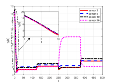
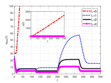
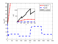
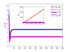
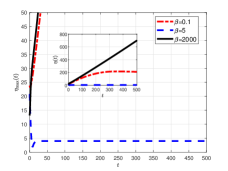
By selecting $\beta=3$ and $L=3$ for Algorithm 1, estimation errors $\eta_{i}(t),i=3,5,10,26$ are provided in Fig. 4 (a). From this figure, we see that there are three time instants, i.e., $t=125,250,375$, around which the error dynamics of the plotted sensors fluctuate. The reason why the error dynamics of one sensor increase lies in two aspects. First, after a certain time instant, this sensor is under attack. If so, its observations will be compromised and the estimation performance of this sensor will be degraded. For example, in Fig. 4 (a), the errors of sensor $5$ after time $t=375$, sensor $10$ after time $t=125$, and sensor $26$ after time $t=250$ all increase for this reason. The second aspect is that after a certain time instant, the neighbor of one senor is under attack. For this sensor, its error will also increase due to the consensus influence. For example, in Fig. 4 (a), the error of sensor $3$ increases after time $t=125$, since a neighbor of sensor $3$, i.e., sensor $10$, is under attack after time $t=125$. The reason that the estimation error of sensor 26 is large in the time interval 250–375 in Fig. 4 (a) is because of two reasons: 1) After $t=250$, sensor 26 is persistently under attack until $t=375$; 2) The communication rate $L=1$ is small. Since the state estimate is affected by the compromised sensor observations, the estimation error will inevitably increase if the information of neighbors is not available in time. However, Algorithm 1 provides a way to improve the estimation performance by increasing the communication rate $L$. In Fig. 4 (b), the relationship between estimation error $\eta(t)$ and communication rate $L$ is studied. The result shows that with the increase of communication rate $L$, estimation error $\eta(t)$ decreases. The connection between estimation error $\eta(t)$ and parameter $\beta$ is studied in Fig. 4 (c) under $L=4$. The figure shows that the estimation error with $\beta=5$ is the smallest within the errors by respectively setting $\beta=0.1,5,2000$. The result conforms to the discussion on the design of $\beta$ which should not be too small or too large in the algorithm setting.

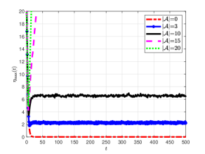
To show the resilience of Algorithm 1, for the case that the attacked sensor set is time-invariant, under $L=4$ and $\beta=5$, we study the relationship between $|\mathcal{A}|$ and $\eta(t)$ in Fig. 6 by randomly choosing a subset of the whole sensors (i.e., $\mathcal{A}$). The result of this figure shows that with the increase of $|\mathcal{A}|$, the estimation error $\eta(t)$ becomes larger. Also, when $|\mathcal{A}|$ is equal to or larger than half sensors, the estimation error is unstable.

123456789101112131415161718192021222324252627282930
(a) $t=1,2,\dots,125$
123456789101112131415161718192021222324252627282930
(b) $t=126,127,\dots,250$
123456789101112131415161718192021222324252627282930
(c) $t=251,252,\dots,375$
123456789101112131415161718192021222324252627282930
(d) $t=376,377,\dots,500$
Figure 3: Sensor network with different sets of attacked sensors over four time intervals.
Refer to caption
(a) The estimation errors of some sensors.
Refer to caption
(b) The relationship between $L$ and $\eta_{\max}(t)$.
Refer to caption
(c) The relationship between $\beta$ and $\eta_{\max}(t)$.
Figure 4: Estimation performance of Algorithm 1 for the sensor networks in Fig. 3.
Refer to caption
(a) The estimation errors of some sensors.
Refer to caption
(b) The relationship between $L$ and $\eta_{\max}(t)$.
Refer to caption
(c) The relationship between $\beta$ and $\eta_{\max}(t)$.
Figure 5: Estimation performance of Algorithm 1 for the sensor network in Fig. 1.
Refer to caption
Figure 6: Resilience of Algorithm 1.
Refer to caption
Figure 7: The estimation error comparison of algorithms.

5-B Secured Distributed Estimation Under Detection

In this subsection, we consider the introduction case in Fig. 1 where the attacked sensor set is time-invariant, with $\mathcal{A}(t)=\mathcal{A}=\{3,12,13,15,23,28\},$ under which the estimation performance of Algorithms 1 and 2 is studied.
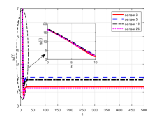
By selecting $\beta=3$ and $L=3$ for Algorithm 1, estimation errors $\eta_{i}(t),i=3,5,10,26$ are provided in Fig. 5 (a). Compared to the result in Fig. 4 (a), the estimation errors of these sensors in Fig. 5 (a) do no fluctuate. Since the attacked sensor set is time-invariant, the estimation errors become steady after transience as shown in the figure. The relationships between parameters $L$, $\beta$ and estimation error $\eta(t)$ are shown in Fig. 5 (b) and (c). Note that in Fig. 5 (b), when $L=0$, estimation error $\eta(t)$ is divergent, since for the attacked sensors, the local observability is violated. Fig. 5 (b) also shows that with the increase of communication rate $L$, the estimation error of Algorithm 1 is decreasing. In Fig. 5 (c), parameter $\beta=5$ can lead to the stable estimation error, while in Fig. 4 (c), the estimation error for parameter $\beta=5$ fluctuates due to the switching of the attacked sensor set.

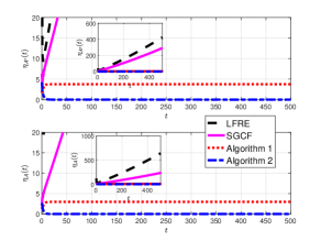
In order to compare with existing algorithms under the situation in Fig. 1, we define the estimation errors for the attacked sensor set and attack-free sensor set, respectively: $\eta_{\mathcal{A}}(t)=\frac{1}{100}\sum_{j=1}^{100}\max_{i\in\mathcal{A}}\left\lVert e_{i}^{j}(t)\right\rVert$, and $\eta_{\mathcal{A}^{c}}(t)=\frac{1}{100}\sum_{j=1}^{100}\max_{i\in\mathcal{A}^{c}}\left\lVert e_{i}^{j}(t)\right\rVert.$ In Fig. 7, the estimation performance of Algorithms 1 and 2 with $L=5$, the local-filtering based resilient estimation (LFRE) [11] and the scalar-gain consensus filter111The filter has the same form as Algorithm 1 but $k_{i}(t)=1$ for $t\geq 1.$ It follows the idea in [33], which did not consider the attack scenario. (SGCF) is compared. The figure shows that Algorithms 1 and 2 provide estimates with stable estimation errors for both attacked sensors and attack-free sensors, but the estimation errors of LFRE and SGCF are divergent. Compared to Algorithm 1, Algorithm 2 provides smaller estimation errors by successfully detecting all the attacked sensors.

6 Conclusion and Future Work

This paper studied the distributed filtering problem for linear time-invariant systems with bounded noise under false-data injection attacks in sensors networks, where a malicious attacker can compromise a time-varying and unknown subset of sensors and manipulate their observations arbitrarily. First, we proposed a distributed saturation-based filter. Then, we provided a sufficient condition to guarantee boundedness of the estimation error. By confining the attacked sensor set to be time-invariant, we then modified the filter by adding an attack detection scheme. Moreover, for the noise-free case, we proved that the state estimate of each sensor asymptotically converges to the system state under certain conditions.

There are some future directions. Since this paper employs a two-time-scale scheme in filter design, it is interesting to develop algorithms which use one communication at each time. Other directions include considering more general systems (e.g., nonlinear systems) and more complex sensor networks (e.g., random or communication-delayed networks).

ACKNOWLEDGMENT

The authors are grateful to the anonymous reviewers for their insightful comments and suggestions.

-A Proof of Lemma 1

First, we prove 2). Due to $t_{0}\in\Gamma$, we have

$\displaystyle F(x_{t_{0}-1})x_{t_{0}-1}+q_{0}=x_{t_{0}}\leq x_{t_{0}-1}.$ (18)

For $t=t_{0}+1$, by (18) and the condition that $F(\cdot)\in[0,1]$ is a monotonically non-decreasing function, we have $x_{t_{0}+1}=F(x_{t_{0}})x_{t_{0}}+q_{0}\leq F(x_{t_{0}-1})x_{t_{0}-1}+q_{0}=x_{t_{0}}.$ By recursively applying the above procedure, we have $\sup_{t\geq t_{0}}x_{t}\leq x_{t_{0}}.$

Next, we prove 1), which trivially holds for $t=t_{0}$. Consider the case of $t>t_{0}$ in the following. If $q_{0}\neq 0$, it follows from (18) that $F(x_{t_{0}-1})\in[0,1)$. Due to $F(x_{t_{0}})\leq F(x_{t_{0}-1})$, we have $F(x_{t_{0}})\in[0,1)$. By 2) and the condition that $F(\cdot)\in[0,1]$ is a monotonically non-decreasing function, we have $F(x_{t-1})\leq F(x_{t_{0}})$. Then $x_{t}\leq F(x_{t_{0}})x_{t-1}+q_{0}$ with $F(x_{t_{0}})\in[0,1)$. Thus, 1) is satisfied by recursively applying the inequality for $t-t_{0}$ times.

Finally, we prove 3). By 1) and the definition of $\limsup$, we have $\limsup\limits_{t\rightarrow\infty}x_{t}=\inf\limits_{t\in\mathbb{Z}^{+}}\sup\limits_{m\geq t}x_{m}\leq\inf\limits_{t\in\Gamma}\sup\limits_{m\geq t}x_{m}\leq\inf\limits_{t\in\Gamma}x_{t}.$

-B Proof of Theorem 1

Let $e_{i}(t)=\tilde{e}(t)+\bar{e}_{i}(t)$, where $\bar{e}_{i}(t):=\hat{x}_{i}(t)-\hat{x}_{avg}$, and $\tilde{e}(t)=\hat{x}_{avg}-x(t),$ and $\hat{x}_{avg}(t):=\frac{1}{N}\sum_{i=1}^{N}\hat{x}_{i}(t)$. Besides, we denote

$\displaystyle X(t)$ $\displaystyle=\textbf{1}_{N}\otimes x(t)\in\mathbb{R}^{Nn},$
$\displaystyle\bar{E}(t)$ $\displaystyle=\left(\bar{e}_{1}^{\sf T}(t),\dots,\bar{e}_{N}^{\sf T}(t)\right)^{\sf T}\in\mathbb{R}^{Nn},$
$\displaystyle Y(t)$ $\displaystyle=\left(y_{1}^{\sf T}(t),\dots,y_{N}^{\sf T}(t)\right)^{\sf T}\in\mathbb{R}^{N},$
$\displaystyle V(t)$ $\displaystyle=\left(v_{1}^{\sf T}(t),\dots,v_{N}^{\sf T}(t)\right)^{\sf T}\in\mathbb{R}^{N},$
$\displaystyle\hat{X}(t)$ $\displaystyle=\left(\hat{x}_{1}^{\sf T}(t),\dots,\hat{x}_{N}^{\sf T}(t)\right)^{\sf T}\in\mathbb{R}^{Nn},$ (19)
$\displaystyle\bar{C}$ $\displaystyle=\operatorname{diag}\{C_{1},\dots,C_{N}\}\in\mathbb{R}^{N\times Nn},$
$\displaystyle\bar{K}(t)$ $\displaystyle=\operatorname{diag}\{k_{1}(t),\dots,k_{N}(t)\}\in\mathbb{R}^{N\times N},$
$\displaystyle P_{Nn}$ $\displaystyle=\frac{1}{N}(\textbf{1}_{N}\otimes I_{n})(\textbf{1}_{N}\otimes I_{n})^{\sf T}\in\mathbb{R}^{Nn\times Nn}.$

The idea for the proof is that we first show $\left\lVert\bar{e}_{i}(t)\right\rVert$ is upper bounded by $p(t)$, and then we prove $\left\lVert\tilde{e}(t)\right\rVert$ is upper bounded by the quantities in 1)–3) of the theorem. The following lemma with a similar proof as in [27] ensures $\left\lVert\bar{e}_{i}(t)\right\rVert\leq p(t)$.

Lemma 2.

Consider Algorithm 1, and let Assumptions 12 hold. If $\alpha=\frac{2}{\lambda_{2}(\mathcal{L})+\lambda_{\max}(\mathcal{L})}$, and $L>\frac{\ln\left\lVert A\right\rVert}{\ln\gamma^{-1}}$, then for $t\geq 0,$

$\displaystyle\left\lVert\bar{E}(t)\right\rVert\leq p(t),$ (20)

where $p(t)$ and $\bar{E}(t)$ are defined in (10) and (-B), respectively.

$\displaystyle\begin{split}&\line(1,0){470.0}\\ &\hat{x}_{avg}(t)=A\hat{x}_{avg}(t-1)+\frac{1}{N}(\textbf{1}_{N}^{\sf T}\otimes I_{n})P_{Nn}\left(I_{Nn}-\alpha(\mathcal{L}\otimes I_{n})\right)^{L}\bar{C}^{\sf T}\bar{K}(t)h(t),\\ &\bar{K}_{\mathcal{J}(t)}=\operatorname{diag}\{k_{1}(t)\mathbb{I}_{1\in\mathcal{J}(t)},\dots,k_{N}(t)\mathbb{I}_{N\in\mathcal{J}(t)}\},\quad\bar{K}_{\mathcal{J}^{c}(t)}=\operatorname{diag}\{k_{1}(t)\mathbb{I}_{1\in\mathcal{J}^{c}(t)},\dots,k_{N}(t)\mathbb{I}_{N\in\mathcal{J}^{c}(t)}\},\\ &\bar{m}_{t}=w(t-1)+\frac{1}{N}(\textbf{1}_{N}^{\sf T}\otimes I_{n})\bar{C}^{\sf T}\bar{K}_{\mathcal{J}(t)}(t)\left(\bar{C}((I_{N}\otimes A)\bar{E}(t-1)-I_{N}\otimes w(t-1))-V(t)\right)\\ &h(t)=Y(t)-\bar{C}(I_{N}\otimes A)\hat{X}(t-1),\quad M_{t}=(I_{n}-\frac{1}{N}\sum_{i\in\mathcal{J}(t)}k_{i}(t)C_{i}^{\sf T}C_{i})A,\quad\tilde{m}_{t}=\frac{1}{N}(\textbf{1}_{N}^{\sf T}\otimes I_{n})\bar{C}^{\sf T}\bar{K}_{\mathcal{J}^{c}(t)}(t)h(t)\\ &\line(1,0){470.0}\end{split}$ (21)

Proof of Theorem 1: It follows from (7) and (9) that $\rho_{1}\leq\rho_{0}=\eta_{0}$, which means that $1\in\Gamma=\{t\geq 1|\rho_{t}\leq\rho_{t-1}\}$. In the following, we prove 1)–3).

Under Assumption 3, there are at least $N-s$ attack-free sensors at each time. Suppose $\mathcal{J}(t)$ is the set of these $N-s$ sensors, i.e., $\mathcal{J}(t)\subseteq\mathcal{A}^{c}(t)$ with $|\mathcal{J}(t)|=N-s$. Denote $\mathcal{J}^{c}(t)=\mathcal{V}\setminus\mathcal{J}(t)$, which satisfies $|\mathcal{J}^{c}(t)|=s$ due to $|\mathcal{V}|=N.$ By Algorithm 1 and the notations in (-B), we have the dynamics of $\hat{x}_{avg}(t)$ in (21). Due to $(\textbf{1}_{N}^{\sf T}\otimes I_{n})P_{Nn}=(\textbf{1}_{N}^{\sf T}\otimes I_{n})\left(I_{Nn}-\alpha(\mathcal{L}\otimes I_{n})\right)^{L}=(\textbf{1}_{N}^{\sf T}\otimes I_{n}),$ we have

$\displaystyle\tilde{e}(t)=$ $\displaystyle M_{t}\tilde{e}(t-1)-\bar{m}_{t}+\tilde{m}_{t},$ (22)

where $M_{t}$, $\tilde{m}_{t}$, and $\bar{m}_{t}$ are given in (21). Note that $\tilde{m}_{t}$ can be rewritten in the following way

$\displaystyle\tilde{m}_{t}=\frac{1}{N}\sum_{i\in\mathcal{J}^{c}(t)}C_{i}^{\sf T}k_{i}(t)(y_{i}(t)-C_{i}A\hat{x}_{i}(t-1)).$

Due to $k_{i}(t)=\min\{1,\frac{\beta}{|y_{i}(t)-C_{i}A\hat{x}_{i}(t-1)|}\}$, it holds that $|k_{i}(t)(y_{i}(t)-C_{i}A\hat{x}_{i}(t-1))|\leq\beta$. Since we assume $\|C_{i}\|=1$ after the system model, it holds that $\|\tilde{m}_{t}\|\leq\frac{1}{N}\sum_{i\in\mathcal{J}^{c}(t)}\|C_{i}^{\sf T}\|\beta\leq|\mathcal{J}^{c}(t)|\frac{\beta}{N}.$ Due to $|\mathcal{J}^{c}(t)|=s$, we have

$\displaystyle\left\lVert\tilde{m}_{t}\right\rVert\leq$ $\displaystyle\frac{s}{N}\beta.$ (23)

Regarding $\bar{m}_{t}$, by Assumption 3 and $k_{i}(t)\leq 1$, we have

$\displaystyle\left\lVert\bar{m}_{t}\right\rVert$ $\displaystyle\leq\left\lVert w(t-1)\right\rVert+\frac{|\mathcal{J}(t)|}{N}(\left\lVert A\right\rVert\left\lVert\bar{E}(t-1)\right\rVert$
$\displaystyle\quad+\left\lVert w(t-1)\right\rVert+b_{v})$
$\displaystyle\leq\frac{N-s}{N}(b_{w}+b_{v}+\left\lVert A\right\rVert p_{0})+b_{w},$ (24)

where the second inequality is obtained by Lemma 2 and $\sup_{t\geq 0}p(t)\leq p_{0}$, where $p_{0}$ is defined in (8). Based on (22)–(-B), we construct the sequence $\{\rho_{t}\}$ in (7). In the following, we prove that $\left\lVert\tilde{e}(t)\right\rVert\leq\rho_{t}$.

At the initial time, i.e., $t=0,$ by Assumption 1, we have $\left\lVert\tilde{e}(0)\right\rVert=\left\lVert\hat{x}_{avg}(0)-x(0)\right\rVert\leq\frac{1}{N}\sum_{i=1}^{N}\left\lVert\hat{x}_{i}(0)-x(0)\right\rVert\leq\eta_{0}.$ Due to $\rho_{0}=\eta_{0}$, $\left\lVert\tilde{e}(t)\right\rVert\leq\rho_{t}$ for $t=0.$ Suppose at time $t-1$, $\left\lVert\tilde{e}(t-1)\right\rVert\leq\rho_{t-1}.$ At time $t$, for $i\in\mathcal{J}(t)$, we consider

$\displaystyle|y_{i}(t)-C_{i}A\hat{x}_{i}(t-1)|$
$\displaystyle\leq$ $\displaystyle\left\lVert A\right\rVert\left\lVert e_{i}(t-1)\right\rVert+b_{w}+b_{v}$
$\displaystyle\leq$ $\displaystyle\left\lVert A\right\rVert(\left\lVert\bar{e}_{i}(t-1)\right\rVert+\left\lVert\tilde{e}(t-1)\right\rVert)+b_{w}+b_{v}$
$\displaystyle\leq$ $\displaystyle\left\lVert A\right\rVert(p_{0}+\rho_{t-1})+b_{w}+b_{v},$ (25)

where the last inequality of (-B) is obtained by noting that $\sup_{t\geq 0}\left\lVert\bar{e}_{i}(t)\right\rVert\leq\sup_{t\geq 0}p(t)\leq p_{0}$ and $p_{0}$ is defined in (8). Recall the form of $k_{i}(t)$, by (-B), for $i\in\mathcal{J}(t)$, we have $k_{i}(t)\geq k^{*}(\rho_{t-1}):=\min\bigg{\{}1,\frac{\beta}{\left\lVert A\right\rVert(p_{0}+\rho_{t-1})+b_{w}+b_{v}}\bigg{\}}>0.$ Then

$\displaystyle\left\lVert M_{t}\right\rVert\leq$ $\displaystyle\left\lVert A\right\rVert\left\lVert\left(I_{n}-\frac{k^{*}(\rho_{t-1})}{N}\sum_{i\in\mathcal{J}(t)}C_{i}^{\sf T}C_{i}\right)\right\rVert$
$\displaystyle\leq$ $\displaystyle\left\lVert A\right\rVert\left(1-\frac{k^{*}(\rho_{t-1})}{N}\lambda_{0}\right).$ (26)

Taking norm on both sides of (22) and considering (7), (23), (-B), and (-B), we have $\left\lVert\tilde{e}(t)\right\rVert\leq\rho_{t}.$

Since the defined $F(\rho_{t})$ in (8) is monotonically non-decreasing function, conclusions 1)–3) of this theorem are obtained by applying the results in Lemma 1, $\left\lVert e_{i}(t)\right\rVert\leq\left\lVert\tilde{e}(t)\right\rVert+\left\lVert\bar{e}_{i}(t)\right\rVert$, and (20).

-C Proof of Theorem 2

1) Sufficiency:

Case 1: For the case $s>0$, we consider $\left\lVert A\right\rVert\in[1,1+\epsilon)$ with $\epsilon=\frac{\lambda_{0}-s}{4(N-\lambda_{0})}$ which is positive due to $\lambda_{0}>s$. If $L$ is sufficiently large, $p_{0}>0$ in (8) will be sufficiently small. Thus, given noise bounds $b_{w}$ and $b_{v}$, considering $N\geq s+\lambda_{0}$, it is feasible to choose sufficiently large $\beta,\eta_{0}$ and $L>\frac{\ln\left\lVert A\right\rVert}{\ln\gamma^{-1}}$, such that

$\displaystyle\begin{split}\beta&\geq(1+\epsilon)(p_{0}+\eta_{0})+b_{w}+b_{v},\\ \beta&\leq\min\left\{(1+\epsilon+\frac{\lambda_{0}-s}{4s})\eta_{0},\frac{N}{s}(\eta_{0}-\frac{Q_{0}}{\epsilon_{1}})\right\},\end{split}$ (27)

where $\epsilon_{1}=\frac{\epsilon}{1+2\epsilon}>0$, and

$\displaystyle Q_{0}:=\frac{N-s}{N}(b_{w}+b_{v}+\left\lVert A\right\rVert p_{0})+b_{w}.$ (28)

By the first inequality and second inequality of (27), we have $k_{0}^{*}=\min\{1,\frac{\beta}{\left\lVert A\right\rVert(p_{0}+\eta_{0})+b_{w}+b_{v}}\}=1$ and $\frac{s\beta}{N\eta_{0}}<1$, respectively. Then

$\displaystyle m_{0}:$ $\displaystyle=\left(1-\frac{s\beta}{N\eta_{0}}\right)\left(1-\frac{k_{0}^{*}\lambda_{0}}{N}\right)^{-1}$
$\displaystyle=\left(\frac{N}{s}-\frac{\beta}{\eta_{0}}\right)\left(\frac{N-\lambda_{0}}{s}\right)^{-1}$
$\displaystyle=1+\left(\frac{\lambda_{0}}{s}-\frac{\beta}{\eta_{0}}\right)\frac{s}{N-\lambda_{0}}$
$\displaystyle\overset{(a)}{\geq}1+\left(\frac{\lambda_{0}}{s}-1-\frac{\lambda_{0}-s}{4s}-\epsilon\right)\frac{s}{N-\lambda_{0}}$
$\displaystyle=1+\frac{3(\lambda_{0}-s)}{4(N-\lambda_{0})}-\frac{\epsilon s}{N-\lambda_{0}}$
$\displaystyle\overset{(b)}{\geq}1+2\epsilon$ (29)

where $(a)$ is obtained by applying the second inequality of (27), and $(b)$ is derived by using $\lambda_{0}-s=4\epsilon(N-\lambda_{0})$ and $s\leq N-\lambda_{0}$. From the second inequality of (27), we obtain

$\displaystyle\vartheta_{0}:=1-\frac{Q_{0}}{\eta_{0}}\left(1-\frac{s\beta}{N\eta_{0}}\right)^{-1}\geq 1-\epsilon_{1}=\frac{1+\epsilon}{1+2\epsilon}.$ (30)

By (-C) and (30), we have $\vartheta_{0}m_{0}\geq 1+\epsilon\geq\left\lVert A\right\rVert$. It is easy to check that $\vartheta_{0}m_{0}\geq\left\lVert A\right\rVert$ is equivalent equation (9). Thus, the sufficiency is satisfied in this case with the above parameters, i.e., $\epsilon=\frac{\lambda_{0}-s}{4(N-\lambda_{0})}$, and $\beta,\eta_{0}$ and $L>\frac{\ln\left\lVert A\right\rVert}{\ln\gamma^{-1}}$ satisfying (27).

Case 2: For the attack-free case, i.e., $s=0$, we consider $\left\lVert A\right\rVert\in[1,1+\epsilon)$ with $\epsilon=\frac{\lambda_{0}}{4N-\lambda_{0}}>0$. Similar to case 1, it is feasible to choose sufficiently large $\beta,\eta_{0}$ and $L>\frac{\ln\left\lVert A\right\rVert}{\ln\gamma^{-1}}$, such that

$\displaystyle\begin{split}2\beta&\geq(1+\epsilon)(p_{0}+\eta_{0})+b_{w}+b_{v},\\ \frac{q_{0}}{\eta_{0}}&\leq\frac{\lambda_{0}}{4N}(1+\epsilon).\end{split}$ (31)

From the first inequality of (31), we see $k_{0}^{*}=\min\{1,\frac{\beta}{\left\lVert A\right\rVert(p_{0}+\eta_{0})+b_{w}+b_{v}}\}\geq\frac{1}{2}$. With $k_{0}^{*}\geq\frac{1}{2}$, it is easy to check that equation (9) is satisfied if $\frac{1}{\left\lVert A\right\rVert}\frac{\eta_{0}-q_{0}}{\eta_{0}}\geq 1-\frac{\lambda_{0}}{2N}$. This inequality is satisfied due to $\left\lVert A\right\rVert\in[1,1+\epsilon)$ and the second inequality of (31). Thus, the sufficiency is satisfied in this case with $\epsilon=\frac{\lambda_{0}}{4N-\lambda_{0}}$, and $\beta,\eta_{0}$ and $L>\frac{\ln\left\lVert A\right\rVert}{\ln\gamma^{-1}}$ satisfying (31).

Note that for $\eta_{0}$ in the two cases above, we are able to make it bigger such that the initial error condition in Assumption  1 holds.

2) Necessity: We use the contradiction method. If $\lambda_{0}>s$ does not hold, i.e., $\lambda_{0}\leq s$. Equation (9) is equivalent to

$\displaystyle\frac{\eta_{0}-q_{0}}{\eta_{0}}\left(1-\frac{k^{*}_{0}\lambda_{0}}{N}\right)^{-1}\geq\left\lVert A\right\rVert\geq 1.$ (32)

If $\frac{s\beta}{N\eta_{0}}\geq 1$, from the form of $q_{0}$ in (8), we have $\eta_{0}<q_{0}$. Then the left-hand side of (32) is negative, which contracts with the right-hand side of (32). Thus, $\frac{s\beta}{N\eta_{0}}<1.$ With the same notations as case 1 of the sufficiency proof, (32) is equivalent to $\vartheta_{0}m_{0}\geq\left\lVert A\right\rVert\geq 1$. Due to $\frac{s\beta}{N\eta_{0}}<1$, we have $\vartheta_{0}<1.$ Then $m_{0}$ has to be larger than 1, which leads to $\frac{s\beta}{N\eta_{0}}<\frac{k^{*}_{0}\lambda_{0}}{N}$. It is equivalent to $\frac{s}{\lambda_{0}}<\frac{k^{*}_{0}\eta_{0}}{\beta}$. Due to $\frac{s}{\lambda_{0}}\geq 1$, we have $\frac{k^{*}_{0}\eta_{0}}{\beta}>1$, which however can not be satisfied due to $k_{0}^{*}=\min\{1,\frac{\beta}{\left\lVert A\right\rVert(p_{0}+\eta_{0})+b_{w}+b_{v}}\}$. Thus, the conjecture $\lambda_{0}\leq s$ is not right, which means $\lambda_{0}>s$.

-D Proof of Theorem 3

First, we prove 1). For $i\in\mathcal{A}^{c}(t)$, by 2) of Theorem 1, we have $\sup\limits_{t\geq t_{0}}\left\lVert e_{i}(t)\right\rVert\leq\rho_{t_{0}}+\sup_{t\geq t_{0}}p(t)$, thus,

$\displaystyle\sup\limits_{t\geq t_{0}+1}|y_{i}(t)-C_{i}A\hat{x}_{i}(t-1)|$
$\displaystyle\leq$ $\displaystyle\left\lVert A\right\rVert\sup\limits_{t\geq t_{0}+1}\left\lVert e_{i}(t-1)\right\rVert+b_{w}+b_{v}$
$\displaystyle\leq$ $\displaystyle\left\lVert A\right\rVert(\rho_{t_{0}}+\sup_{t\geq t_{0}}p(t))+b_{w}+b_{v}.$

If (12) holds, by Algorithm 1, all the observations of the attack-free sensors will eventually not be saturated, i.e., $k_{i}(t)=1,\forall i\in\mathcal{A}^{c}(t),t\geq t_{0}+1.$

Next, we prove 2). By 1) of this theorem, for $i\in\mathcal{A}^{c}(t)$, we have $k_{i}(t)=1$, $\forall t>t_{0}$, then $\left\lVert M_{t}\right\rVert\leq\varpi,$ where $M_{t}$ is defined in (21). According to the error dynamics in (22) and inequalities (23)–(-B), the upper bound of $\left\lVert\tilde{e}(t)\right\rVert$ is obtained by applying Lemma 1. It follows from (-B) that the bound is tighter than the one in 1) of Theorem 1. Due to $\left\lVert e_{i}(t)\right\rVert\leq\left\lVert\tilde{e}(t)\right\rVert+\left\lVert\bar{e}_{i}(t)\right\rVert$ and (20), the upper bound of $\left\lVert e_{i}(t)\right\rVert$ is obtained.

Finally, we prove 3). By the real-time upper bound of the estimation error, it is straightforward to have its limit superior. Next, we prove the limit superior bound is no larger than the one in 3) of Theorem 1, i.e., $\frac{q_{0}}{1-\varpi}\leq\inf\limits_{t_{0}\in\Gamma}\rho_{t_{0}}.$ Employing the properties $\inf x+y\geq\inf x+\inf y$ and $\inf xy\geq\inf x\inf y$ for $x,y>0$ on $F(\rho_{t_{0}})\rho_{t_{0}}+q_{0}=\rho_{t_{0}+1}\leq\rho_{t_{0}}$ yields

$\displaystyle\inf\limits_{t_{0}\in\Gamma}\rho_{t_{0}}$ $\displaystyle\geq\frac{q_{0}}{1-\inf\limits_{t_{0}\in\Gamma}F(\rho_{t_{0}})}$
$\displaystyle\overset{(a)}{\geq}\frac{q_{0}}{1-\left\lVert A\right\rVert\left(1-\frac{1}{N}\lambda_{0}\right)}$
$\displaystyle\geq\frac{q_{0}}{1-\varpi},$

where $(a)$ holds by considering the expression of $F(\cdot)$ in (8).

-E Proof of Proposition 2

First, we consider the case of $\left\lVert A\right\rVert<1$. By applying 1) of Theorem 1 and choosing $t_{0}=1$ and $\bar{q}_{0}=b_{w}+\max\{\beta,b_{w}+b_{v}+\left\lVert A\right\rVert p_{0}\}$, we have (13). From (6) and (8), we see that $F(\eta_{0})$ is a monotonically non-decreasing function w.r.t. $s$. Thus $f(s)$ is a monotonically non-decreasing function w.r.t. $s$.

Second, we consider the case of $\left\lVert A\right\rVert\geq 1$. In the case, we have (13), by applying 1) of Theorem 1, and by choosing $t_{0}=1$ and $\bar{q}_{0}=q_{0}$. Next, we show the $f(s)$ is a monotonically non-decreasing function w.r.t. $s$. As discussed above that $F(\eta_{0})$ is a monotonically non-decreasing function w.r.t. $s$, we just need to prove that $q_{0}$ is a monotonically non-decreasing function w.r.t. $s$. This is obviously ensured if $\beta>b_{w}+b_{v}+\left\lVert A\right\rVert p_{0}$. Next, we prove this point by contradiction. In other words, we assume $\beta\leq b_{w}+b_{v}+\left\lVert A\right\rVert p_{0}$. Note that (9) is equivalent to

$\displaystyle 1-k^{*}(\eta_{0})\frac{\lambda_{0}}{N}\leq\frac{1}{\left\lVert A\right\rVert}\left(1-\frac{q_{0}}{\eta_{0}}\right).$ (33)

Due to $\beta\leq b_{w}+b_{v}+\left\lVert A\right\rVert p_{0}$, we have $q_{0}\geq\beta+b_{w}$. Then a necessary to ensure (33) is

$\displaystyle 1-k^{*}(\eta_{0})\frac{\lambda_{0}}{N}\leq\frac{1}{\left\lVert A\right\rVert}\left(1-\frac{\beta+b_{w}}{\eta_{0}}\right).$ (34)

It follows from (8) that $k^{*}(\eta_{0})=\frac{\beta}{\left\lVert A\right\rVert(p_{0}+\eta_{0})+b_{w}+b_{v}}$. By substituting $k^{*}(\eta_{0})$ into (34), we obtain

$\displaystyle\frac{\beta}{\left\lVert A\right\rVert(p_{0}+\eta_{0})+b_{w}+b_{v}}\frac{\lambda_{0}}{N}\geq\frac{\beta+b_{w}+(\left\lVert A\right\rVert-1)\eta_{0}}{\left\lVert A\right\rVert\eta_{0}},$

which can not be satisfied due to $\lambda_{0}\leq N$ and $1\leq\left\lVert A\right\rVert.$ Therefore, the assumption $\beta\leq b_{w}+b_{v}+\left\lVert A\right\rVert p_{0}$ does not hold.

-F Proof of Theorem 4

The proof is similar to the proofs of Theorems 13. In the following, we just show the main points of this proof.

Given a time $T>0$ and the maximal number of the detected sensors at time $t$, i.e., $d(T)$, similar to the proof of Theorem 1, for $\forall t\geq T$, we construct the following sequence $\{\bar{\rho}_{t}\in\mathbb{R}|\bar{\rho}_{t}\}$ in (17). It is straightforward to prove that for $\forall t\geq T$, $\left\lVert\tilde{e}(t)\right\rVert\leq\bar{\rho}_{t}$, where $\tilde{e}(t)=\frac{1}{N}\sum_{i=1}^{N}\hat{x}_{i}(t)-x(t)$. Next, we study the relationship between $\bar{\rho}_{t}$ in (17) and $\rho_{t}$ in (7). Due to $\bar{\rho}_{T}=\rho_{T}$, we have $\bar{\rho}_{T+1}=\rho_{T+1}-\frac{d(T)\beta}{N}.$ Then, for $t=T+2,$ we have

$\displaystyle\bar{\rho}_{T+2}$ $\displaystyle=F(\bar{\rho}_{T+1})\rho_{T+1}+q_{0}-(F(\bar{\rho}_{T+1})+1)\frac{d(T)\beta}{N}$
$\displaystyle\leq\rho_{T+2}-(F_{*}+1)\frac{d(T)\beta}{N}.$

where $F_{*}=\inf\limits_{t_{0}\in\bar{\Gamma}}F(\bar{\rho}_{t_{0}})\in[0,1)$, and $\bar{\Gamma}=\{t\geq T|\bar{\rho}_{t}\leq\bar{\rho}_{t-1}\}$. By recursively applying the above operation, for $t\geq T$, we obtain

$\displaystyle\bar{\rho}_{t}\leq\rho_{t}-\frac{d(T)\beta}{N}\left(\frac{1-F_{*}^{t-T}}{1-F_{*}}\right).$

Then by Lemma 1 and Theorem 1, we have $\limsup\limits_{t\rightarrow\infty}\left\lVert\tilde{e}(t)\right\rVert\leq\inf\limits_{t_{0}\in\Gamma}\rho_{t_{0}}-\frac{d(T)\beta}{N(1-F_{*})}.$ Thus, the first conclusion holds by applying Lemma 1, $\left\lVert e_{i}(t)\right\rVert\leq\left\lVert\tilde{e}(t)\right\rVert+\left\lVert\bar{e}_{i}(t)\right\rVert$, and (20).

-G Proof of Theorem 5

Under condition 1), owing to the connectivity of network $\mathcal{G}$, there is a common time $\tilde{t}\geq\hat{t}_{0}$, such that $d_{j}(\tilde{t})=s,\forall j\in\mathcal{V}$. For $t\geq\tilde{t}$, all the observations of the attacked sensors are discarded. Then, we have the compact form of recursive state estimates of Algorithm 2 in the following

$\displaystyle\hat{X}(t)=$ $\displaystyle\left(I_{Nn}-\alpha(\mathcal{L}\otimes I_{n})\right)^{L}\bigg{[}(I_{N}\otimes A)\hat{X}(t-1)$
$\displaystyle+\bar{C}^{\sf T}\bar{K}_{\mathcal{A}^{c}}(Y(t)-\bar{C}(I_{N}\otimes A)\hat{X}(t-1))\bigg{]}.$ (35)

Let $\bar{E}(t)=\hat{X}(t)-\textbf{1}_{N}\otimes\hat{x}_{avg}(t)$, i.e., $\bar{E}(t)=[\bar{e}_{1}^{\sf T}(t),\dots,\bar{e}_{N}^{\sf T}(t)]^{\sf T}.$ By referring to [27], we have

$\displaystyle\left\lVert\bar{E}(t+1)\right\rVert$
$\displaystyle\leq$ $\displaystyle\left\lVert(I_{N}\otimes A)\right\rVert\left\lVert\left(I_{Nn}-\alpha(\mathcal{L}\otimes I_{n})-P_{Nn}\right)^{L}\bar{E}(t)\right\rVert$
$\displaystyle+\big{\|}(I_{Nn}-P_{Nn})\left(I_{Nn}-\alpha(\mathcal{L}\otimes I_{n})\right)^{L}$
$\displaystyle\qquad\bar{C}^{\sf T}\bar{K}_{\mathcal{A}^{c}}(Y(t)-\bar{C}(I_{N}\otimes A)\hat{X}(t-1))\big{\|}$
$\displaystyle\leq$ $\displaystyle 2\left\lVert A\right\rVert\gamma^{L}\left\lVert\bar{E}(t)\right\rVert+\left\lVert A\right\rVert\gamma^{L}\sqrt{N-s}\left\lVert\tilde{e}(t)\right\rVert.$ (36)

Similar to (22), for $i\in\mathcal{A}^{c}$, $t\geq\tilde{t}$, $k_{i}(t)=1$, we have $\tilde{e}(t+1)=M_{21}\tilde{e}(t)-M_{22}\bar{E}(t),$ where $M_{21}=\left(I_{n}-\frac{1}{N}\sum_{i\in\mathcal{A}^{c}}C_{i}^{\sf T}C_{i}\right)A$ and $M_{22}=\frac{1}{N}(\textbf{1}_{N}^{\sf T}\otimes I_{n})\bar{C}^{\sf T}\bar{K}_{\mathcal{A}^{c}}\bar{C}(I_{N}\otimes A).$ Then it holds that

$\displaystyle\left\lVert\tilde{e}(t+1)\right\rVert\leq\tau_{0}\left\lVert\bar{E}(t)\right\rVert+\varpi\left\lVert\tilde{e}(t)\right\rVert,$ (37)

where $\varpi$ is given in Theorem 3. By (-G) and (37), if the matrix $\left(\begin{smallmatrix}2\left\lVert A\right\rVert\gamma^{L}&\left\lVert A\right\rVert\gamma^{L}\sqrt{N-s}\\ \tau_{0}&\varpi\end{smallmatrix}\right)$ is Schur stable, $\left\lVert\tilde{e}(t)\right\rVert$ and $\left\lVert\bar{E}(t)\right\rVert$ go to zero asymptotically. Thus, $\left\lVert e_{i}(t)\right\rVert$ is convergent to zero as time goes to infinity.

References

  • [1] G. Battistelli, L. Chisci, G. Mugnai, A. Farina, and A. Graziano, “Consensus-based linear and nonlinear filtering,” IEEE Transactions on Automatic Control, vol. 60, no. 5, pp. 1410–1415, 2015.
  • [2] Q. Liu, Z. Wang, X. He, and D. Zhou, “Event-based distributed filtering with stochastic measurement fading,” IEEE Transactions on Industrial Informatics, vol. 11, no. 6, pp. 1643–1652, 2015.
  • [3] F. Pasqualetti, F. Dörfler, and F. Bullo, “Attack detection and identification in cyber-physical systems,” IEEE Transactions on Automatic Control, vol. 58, no. 11, pp. 2715–2729, 2013.
  • [4] X. Ren, Y. Mo, J. Chen, and K. H. Johansson, “Secure state estimation with Byzantine sensors: A probabilistic approach,” IEEE Transactions on Automatic Control, vol. 65, no. 9, pp. 3742–3757, 2020.
  • [5] H. Fawzi, P. Tabuada, and S. Diggavi, “Secure estimation and control for cyber-physical systems under adversarial attacks,” IEEE Transactions on Automatic control, vol. 59, no. 6, pp. 1454–1467, 2014.
  • [6] M. Pajic, I. Lee, and G. J. Pappas, “Attack-resilient state estimation for noisy dynamical systems,” IEEE Transactions on Control of Network Systems, vol. 4, no. 1, pp. 82–92, 2017.
  • [7] M. Pajic, J. Weimer, N. Bezzo, O. Sokolsky, G. J. Pappas, and I. Lee, “Design and implementation of attack-resilient cyberphysical systems: With a focus on attack-resilient state estimators,” IEEE Control Systems Magazine, vol. 37, no. 2, pp. 66–81, 2017.
  • [8] Y. Shoukry, P. Nuzzo, A. Puggelli, A. L. Sangiovanni-Vincentelli, S. A. Seshia, and P. Tabuada, “Secure state estimation for cyber-physical systems under sensor attacks: A satisfiability modulo theory approach,” IEEE Transactions on Automatic Control, vol. 62, no. 10, pp. 4917–4932, 2017.
  • [9] Y. Shoukry, M. Chong, M. Wakaiki, P. Nuzzo, A. Sangiovanni-Vincentelli, S. A. Seshia, J. P. Hespanha, and P. Tabuada, “SMT-based observer design for cyber-physical systems under sensor attacks,” ACM Transactions on Cyber-Physical Systems, vol. 2, no. 1, p. 5, 2018.
  • [10] D. Han, Y. Mo, and L. Xie, “Convex optimization based state estimation against sparse integrity attacks,” IEEE Transactions on Automatic Control, vol. 64, no. 6, pp. 2383–2395, 2019.
  • [11] A. Mitra and S. Sundaram, “Byzantine-resilient distributed observers for LTI systems,” Automatica, vol. 108, p. 108487, 2019.
  • [12] A. Mitra, J. A. Richards, S. Bagchi, and S. Sundaram, “Resilient distributed state estimation with mobile agents: overcoming Byzantine adversaries, communication losses, and intermittent measurements,” Autonomous Robots, vol. 43, no. 3, pp. 743–768, 2019.
  • [13] L. Su and S. Shahrampour, “Finite-time guarantees for Byzantine-resilient distributed state estimation with noisy measurements,” IEEE Transactions on Automatic Control, vol. 65, no. 9, pp. 3758–3771, 2020.
  • [14] P. Blanchard, R. Guerraoui, J. Stainer, and E. M. EI Mhamdi, “Machine learning with adversaries: Byzantine tolerant gradient descent,” in Advances in Neural Information Processing Systems, pp. 119–129, 2017.
  • [15] M. Deghat, V. Ugrinovskii, I. Shames, and C. Langbort, “Detection and mitigation of biasing attacks on distributed estimation networks,” Automatica, vol. 99, pp. 369–381, 2019.
  • [16] Y. Chen, S. Kar, and J. M. F. Moura, “Resilient distributed estimation: Sensor attacks,” IEEE Transactions on Automatic Control, vol. 64, no. 9, pp. 3772–3779, 2019.
  • [17] Y. Chen, S. Kar, and J. M. Moura, “Resilient distributed parameter estimation with heterogeneous data,” IEEE Transactions on Signal Processing, vol. 67, no. 19, pp. 4918–4933, 2019.
  • [18] L. An and G.-H. Yang, “Distributed secure state estimation for cyber–physical systems under sensor attacks,” Automatica, vol. 107, pp. 526–538, 2019.
  • [19] M. S. Chong, M. Wakaiki, and J. P. Hespanha, “Observability of linear systems under adversarial attacks,” in American Control Conference, pp. 2439–2444, IEEE, 2015.
  • [20] B. Chen, D. W. Ho, W.-A. Zhang, and L. Yu, “Distributed dimensionality reduction fusion estimation for cyber-physical systems under DoS attacks,” IEEE Transactions on Systems, Man, and Cybernetics: Systems, vol. 49, no. 2, pp. 455–468, 2017.
  • [21] F. Boem, A. J. Gallo, G. Ferrari-Trecate, and T. Parisini, “A distributed attack detection method for multi-agent systems governed by consensus-based control,” in IEEE Conference on Decision and Control, pp. 5961–5966, IEEE, 2017.
  • [22] A. J. Gallo, M. S. Turan, F. Boem, T. Parisini, and G. Ferrari-Trecate, “A distributed cyber-attack detection scheme with application to DC microgrids,” IEEE Transactions on Automatic Control, 2020.
  • [23] N. Forti, G. Battistelli, L. Chisci, S. Li, B. Wang, and B. Sinopoli, “Distributed joint attack detection and secure state estimation,” IEEE Transactions on Signal and Information Processing over Networks, vol. 4, no. 1, pp. 96–110, 2018.
  • [24] Y. Nakahira and Y. Mo, “Attack-resilient $\mathcal{H}_{2}$, $\mathcal{H}_{\infty}$, and $\mathcal{H}_{1}$ state estimator,” IEEE Transactions on Automatic Control, vol. 63, no. 12, pp. 4353–4360, 2018.
  • [25] J. G. Lee, J. Kim, and H. Shim, “Fully distributed resilient state estimation based on distributed median solver,” IEEE Transactions on Automatic Control, vol. 65, no. 9, pp. 3935–3942, 2020.
  • [26] X. He, X. Ren, H. Sandberg, and K. H. Johansson, “Secure distributed filtering for unstable dynamics under compromised observations,” in IEEE Conference on Decision and Control, pp. 5344–5349, IEEE, 2019.
  • [27] X. He, X. Ren, H. Sandberg, and K. H. Johansson, “Design of secure filters under attacked measurements: A saturation method,” in https://www.researchgate.net/publication/340579534, 2020.
  • [28] M. Mesbahi and M. Egerstedt, Graph theoretic methods in multiagent networks. Princeton University Press, 2010.
  • [29] A. Mitra and S. Sundaram, “Secure distributed state estimation of an LTI system over time-varying networks and analog erasure channels,” in American Control Conference, pp. 6578–6583, IEEE, 2018.
  • [30] C. Zhao, J. He, and J. Chen, “Resilient consensus with mobile detectors against malicious attacks,” IEEE Transactions on Signal and Information Processing over Networks, vol. 4, no. 1, pp. 60–69, 2017.
  • [31] Y. Shoukry and P. Tabuada, “Event-triggered state observers for sparse sensor noise/attacks,” IEEE Transactions on Automatic Control, vol. 61, no. 8, pp. 2079–2091, 2016.
  • [32] Z. Guo, D. Shi, K. H. Johansson, and L. Shi, “Optimal linear cyber-attack on remote state estimation,” IEEE Transactions on Control of Network Systems, vol. 4, no. 1, pp. 4–13, 2017.
  • [33] U. A. Khan and A. Jadbabaie, “Collaborative scalar-gain estimators for potentially unstable social dynamics with limited communication,” Automatica, vol. 50, no. 7, pp. 1909–1914, 2014.