Quasi-Orthogonal Z-Complementary Pairs and Their Applications in Fully Polarimetric Radar Systems

Abstract

One objective of this paper is to propose a novel class of sequence pairs, called “quasi-orthogonal Z-complementary pairs (QOZCPs)”, each depicting Z-complementary property for their aperiodic auto-correlation sums and also having a low correlation zone when their aperiodic cross-correlation is considered. Construction of QOZCPs based on Successively Distributed Algorithms under Majorization Minimization (SDAMM) is presented. Another objective of this paper is to apply the proposed QOZCPs in fully polarimetric radar systems and analyse the corresponding ambiguity functions. It turns out that QOZCP waveforms are much more Doppler resilient than the known Golay complementary waveforms.

I Introduction

This paper introduces a novel class of sequence pairs called “quasi-orthogonal Z-complementary pairs (QOZCPs)” and their applications in designing Doppler resilient waveforms in polarimetric radar systems. In what follows, we first review the state-of-the-art on pairs of sequences and Doppler resilient waveforms in polarimetric radar systems, then introduce our contributions in this work.

I-A Sequence pairs

Research on designing sequence pairs with good correlation properties started in early 1950’s when M. J. Golay proposed Golay complementary pairs (GCPs), in his work on multislit spectrometry [1]. GCPs are sequence pairs, each having zero aperiodic auto-correlation sums at every out-of-phase time-shifts [1]. Since then a lot of works have been done on analysing the properties and systematic constructions of the GCPs [2, 3, 4, 5]. However, binary GCPs are available only for lengths of the form $2^{\alpha}10^{\beta}26^{\gamma}$ (where $\alpha$, $\beta$ and $\gamma$ are non-negative integers) [3]. In search of binary sequence pairs of other lengths, depicting similar properties to that of the GCPs, Fan et al. [6] proposed binary Z-complementary pairs (ZCPs). ZCPs are sequence pairs having zero auto-correlation sums for each time-shifts within a certain region around the in-phase position, called the zero-correlation-zone (ZCZ) [6]. ZCPs are available for many more lengths as compared to GCPs [6]. Systematic constructions of ZCPs based on insertion method and generalised Boolean functions for even and odd-lengths have also been extensively studied [7, 8, 9, 10, 11, 12]. In 2013, Gong et al. considered the periodic auto-correlation of a single Golay sequence and proposed a systematic construction such that each of the sequence have a zero auto-correlation zone [13]. This property plays a very important role in the synchronization and detection of signals. Recently in 2018, Chen et al. [14] further studied the zero periodic cross-correlation of the GCPs and proposed a new class of sequence sets, namely Golay-ZCZ sets. However, the aperiodic cross-correlation of the GCPs was never been considered till date.

Beside the theoretical approaches for the systematic constructions of the sequence pairs, numerous numerical approaches are also proposed till date, beginning with the work of Groot et al. [15] in 1992. Groot et al. related the problem of optimizing the merit factor of a sequence with thermodynamics and introduced some evolutionary strategies using optimization tools to get binary sequences having low auto-correlation. Since the merit factor of a sequence is highly multimodal (i.e., it may have multiple local maxima) stochastic optimization algorithms had been used for its maximization [15]. However, for large values of $N$, the computational complexity of these algorithms become very high. To overcome this, Stoica et al. made a remarkable progress and introduced several cyclic algorithms (CAs), namely CA-pruned (CAP) [16], CA-new (CAN) [16], and Weighted CAN (We-CAN) [16] to design sequences with low aperiodic autocorrelation. To generate the sequences with low periodic correlations, the authors also proposed periodic CAN (PeCAN) [17]. To design waveforms with arbitrarily spectral shapes, PeCAN has been modified as the SHAPE algorithm [18]. Inspired by the ideas of [16], Soltanalian et al. [19] proposed a CAN algorithm for complementary sets and termed it as CANARY. In 2012, Soltanalian et al. proposed a computational framework based on an iterative twisted approximation (ITROX) [20] and a set of associated algorithms to generate sequences with good periodic/aperiodic correlation properties. In another work, to minimize the correlation magnitudes in desired intervals, in 2013, Li et al. [21] proposed an approach based on iterative spectral approximation algorithm (ISAA) and derivative-based non-linear optimization algorithms. Gradient based algorithms were proposed in [22, 23, 24, 25] to design sequences with good correlation properties, in the frequency domain.

Meanwhile, in 2015, Song et al. [26] proposed an algorithm to directly minimize the periodic/aperiodic correlation magnitudes at out-of-phase time-shifts, using the general majorization-minimization (MM) method. On the other hand Liang et al. [27] proposed unimodular sequence design using alternating direction method of multipliers (ADMM). ADMM is a superior optimization technique as it decomposes a constrained convex optimization problem into multiple smaller sub-problems whose solutions are coordinated to find the global optimum. This form of decomposition-coordination procedure allows parallel and/or distributed processing, and thus is well suited to the handling big data. Second, in spite of employing iterations in the parameter updating process, it provides superior convergence properties.

It should be noted that, designing of unimodular sequences using various optimization techniques is a decade old problem. However, the problem of designing complementary sequences considering the aperiodic cross-correlation among the sequences have not been considered before.

I-B Doppler resilient waveforms in polarimetric radar systems

Fully polarimetric radar systems are equipped with vertically/ horizontally $(V/H)$ dual-dipole elements at every antenna to make sure the simultaneous occurrence of transmitting and receiving on two orthogonal polarizations [28, 29, 30]. The essential ability of polarimetric radar systems is to capture the scattering matrix which contains polarization properties of the target. The scattering matrix can be given as follows,

$$\mathbf{H}=\begin{bmatrix}h_{VV}&h_{VH}\\ h_{HV}&h_{HH}\end{bmatrix},$$ (1)

where $h_{VH}$ denotes the target scattering coefficient that indicates the polarization change from $H$ (horizontally polarized incident field) into $V$ (vertical polarization channel).

The elements of the scattering matrix are estimated by analysing the auto-ambiguity functions (AAF) and cross-ambiguity functions (CAF) which are the matched filter outputs of the received signal with the transmitted waveforms. Owing to its ideal ambiguity plot at desired delays waveforms with impulse-like autocorrelation functions play an important role in radar applications. Phase coding is a commonly used to generate waveforms with impulse-like auto-correlations. Due to its ideal auto-correlation sum properties Howard et al. [31] and Calderbank et al. [28] combined Golay complementary waveforms with Alamouti signal processing to enable pulse compression for multichannel and fully polarimetric radar systems. One of the main drawbacks of waveforms phase coded with complementary sequences is that its effective ambiguity function is highly sensitive to Doppler shifts. Since then, several works have been done [32, 33, 34] to design waveforms using sequences with good correlation properties which can exhibit some tolerance to Doppler shift. Working in this direction Pezeshki et al. [29] made a remarkable progress in 2008, by designing Doppler resilient waveforms using Golay complementary sets. In [29] the transmission is determined by Alamouti coding and Prouhet-Thue-Morse (PTM) sequences. Extending further Tang et al. [35] proposed Doppler resilient complete complementary code in multiple-input multiple-output (MIMO) radar by using generalised PTM sequences. Since, complementary sequences are not available for all lengths, in search of other sequences to design Doppler resilient waveforms, Wang et al. [36] proposed Z-complementary waveforms using equal sums of (like) powers (ESP) Sequences.

However, one of the major drawbacks of [31, 28, 29] is that, the authors did not consider to design the dual-orthogonal waveforms for polarimetric radar systems. Although fully polarimetric radar systems simultaneously transmit and receive waveforms on two orthogonal polarizations, however, only this property does not help to extract the co- and cross-polarized scatter matrix elements [37, 38]. Therefore in polarimetric radar with simultaneous measurement of scattering matrix elements the waveform need to have an extra orthogonality in addition to polarization orthogonality. Waveforms having two such orthogonality are called dual orthogonal waveforms.

I-C Contributions

One objective of this paper is to propose a novel class of sequence pairs, called “quasi-orthogonal Z-complementary pairs (QOZCPs)”, each depicting Z-complementary property for their aperiodic auto-correlation sums and also having a low correlation zone when their aperiodic cross-correlation is considered. Construction of QOZCPs based on Successively Distributed Algorithms under Majorization Minimization (SDAMM) are presented. Another objective of this paper is to apply the proposed QOZCPs in fully polarimetric radar systems and analyse the corresponding ambiguity functions. To be more precise, the contributions of this paper can be listed as follows:

1. New pairs of sequences called QOZCPs are proposed.

2. An efficient successively distributed algorithm under the MM framework is proposed. SDAMM transform a difficult optimization problem of two variables into two parallel sub-problems of a single variable. Each sub-problem has a closed-form so that the complexity is reduced significantly. Using SDAMM, we construct QOZCPs of any lengths.

3. Extending the works of Pezeshki et al. we propose a Doppler resilient dual orthogonal waveform based on QOZCPs which can be used to efficiently estimate the co- and cross- polarised scatter matrix elements.

4. We compare the ambiguity plots of the proposed QOZCPs with the ambiguity plots of existing DR-GCPs and show that QOZCPs performs better while comparing the CAF plot.

I-D Organization

The rest of the paper is organised as follows. In section II, along with the preliminaries the definition of the QOZCP is proposed. The objective function for the construction of the proposed QOZCPs is derived. In Section III, SADMM algorithm is proposed to solve the optimization problem. In Section IV, we have explained the application of the proposed QOZCPs in radar waveform design. In section V, the numerical experiments are given, where we have compared the ambiguity plots of the proposed QOZCPs with the ambiguity plots of DR-GCPs. Finally, we have given some concluding remarks in section VI.

II QOZCP and Problem Formation

In this section, we will propose the definition and the corresponding properties of QOZCPs. Throughout this paper, the entries of QOZCPs are complex $q$-th roots of unity (unimodular). Then we formally define QOZCPs as follows.

II-A Notations

• $\mathbf{x}^{T}$ and $\mathbf{x}^{H}$ denote the transpose and the Hermitian transpose of vector $\mathbf{x}$, respectively.

• $|x_{l}|$ and $x_{l}^{*}$ denote the modulus of $x_{l}$ and conjugate of $x_{l}$ respectively, where $x_{l}$ is the entries of $\mathbf{x}$.

• $\circ$ denotes the Hadamard product.

• $C_{xy}(k)$ denotes the aperiodic cross-correlation function of $\mathbf{x}=[x_{0},x_{1},\cdots,x_{L-1}]$ and $\mathbf{y}=[y_{0},y_{1},\cdots,y_{L-1}]$, i.e.,

  $$C_{xy}(k)=\left\{\begin{aligned} \sum_{l=0}^{L-k-1}x_{l}y_{l+k}^{*},\quad k\geq 0\\ \sum_{l=0}^{L+k-1}x_{l-k}y_{l}^{*},\quad k<0.\\ \end{aligned}\right.$$ (2)

• $C_{x}(k)$ denotes the aperiodic auto-correlation function of $\mathbf{x}=[x_{0},x_{1},\cdots,x_{L-1}]$, i.e., $C_{x}(k)=C_{xx}(k)$.

• $X(z)$ denotes z-transform of $\mathbf{x}$, i.e., $X(z)=x_{0}+x_{1}z^{-1}+\cdots+x_{L-1}z^{-(L-1)}$.

Definition 1

A pair of length-$L$ sequences $(\mathbf{x},\mathbf{y})$ is called a $(L,Z)$-QOZCP, if

$$\begin{split}&\textit{C}1:|C_{x}(k)+C_{y}(k)|\leq\epsilon,\mathrm{for\,\,any}\,\,0<|k|<Z,\\ &\textit{C}2:|C_{xy}(k)|\leq\epsilon,\mathrm{for\,\,any}\,\,|k|<Z,\end{split}$$

where $\epsilon$ is a very small positive real number which is very close to zero.

Remark: since $C_{yx}(-k)=C_{xy}^{*}(k)$ and $|C_{xy}(k)|\leq\epsilon$, then $|C_{yx}(k)|\leq\epsilon$ for any $|k|<Z$.

According to Definition 1, it can be observed that each QOZCP has low zero correlation zones when the ACFs’ sum and the CCF are considered. It is noted that the nonzero values in the low zero autocorrelation zone are very close to zero. We illustrate the correlation properties of $(L,Z)$-QOZCP with $\epsilon=0$ in Fig. 1. Following this definition of sequence, the task of constructing QOZCPs is transformed into equivalent optimization problems. The optimization problem will be formulated after introducing the objective function and constraints.

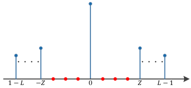
(a) $|C_{x}(\tau)+C_{y}(\tau)|$

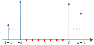
(b) $|C_{xy}(\tau)|$

Figure 1: Illustrative plots for the correlation properties of (L,Z)-QOZCP

II-B Objective Function

We have already introduced the desired sequence pair. In order to find it, unified metrics named the Weighted Complementary Integrated Sidelobe Level (WCISL) and the Weighted Cross-Correlation Integrated Level (WCCIL) are proposed in the following definitions.

Definition 2: The Weighted Complementary Integrated Sidelobe Level (WCISL) of a sequence pair $(\mathbf{x},\mathbf{y})$ is defined as

$$\mathrm{WCISL}=\sum_{k=1}^{L-1}w_{k}|C_{x}(k)+C_{y}(k)|^{2}.$$ (3)

Definition 3: The weighted cross-correlation integrated level(WCCIL) of $\mathbf{x}$, $\mathbf{y}$ is given by

$$\mathrm{WCCIL}=\sum_{k=0}^{L-1}\tilde{w}_{k}|{C_{xy}}(k)|^{2},$$ (4)

where $C_{x}(k)$ and $C_{xy}(k)$ are the auto-correlation function of $\mathbf{x}$ and the cross-correlation function of $\mathbf{x},\mathbf{y}$, respectively. Besides, $w_{-k}=w_{k}$, $w_{0}=0$, $\tilde{w}_{-k}=w_{k}$, $\tilde{w}_{0}\neq 0$.

The expressions of WCISL and WCCIL can also be transformed into the following expressions,

$$\begin{split}&\mathrm{WCISL}=\sum_{k=1}^{L-1}w_{k}(|\mathbf{x}^{H}\mathbf{U}_{k}\mathbf{x}+\mathbf{y}^{H}\mathbf{U}_{k}\mathbf{y}|^{2}),\\ &\mathrm{WCCIL}=\sum_{k=0}^{L-1}w_{k}|\mathbf{x}^{H}\mathbf{U}_{k}\mathbf{y}|^{2},\end{split}$$ (5)

where $\mathbf{U}_{k}$ [39] is an $N\times N$ Toeplitz matrix with 1 in $k$-th diagonal and 0 in the other positions.

To satisfy the conditions, i.e., C1 and C2 at the same time, WCISL and WCCIL should be considered together. Then the objective function is written as

$$\begin{split}\alpha\sum_{k=1}^{L-1}w_{k}(|\mathbf{x}^{H}\mathbf{U}_{k}\mathbf{x}&+\mathbf{y}^{H}\mathbf{U}_{k}\mathbf{y}|^{2})+(1-\alpha)\sum_{k=0}^{L-1}w_{k}|\mathbf{x}^{H}\mathbf{U}_{k}\mathbf{y}|^{2},\end{split}$$ (6)

which will be minimized within a constraint set.

II-C Constraints of Interest

Usually, the sequences to be designed have limited energy [40]. In addition, the large PAPR results in a difficult dilemma between power efficiency and signal distortion [41]. Therefore, constraints of energy and PAPR should be considered as follows:

1) Energy Constraint: The energy of $\mathbf{x}$ and $\mathbf{y}$ should be constrained to a given power $p_{e}$, i.e.,

$$||\mathbf{x}||^{2}=p_{e},||\mathbf{y}||^{2}=p_{e},$$ (7)

where $p_{e}$ is not larger than $L$(L is the length of $\mathbf{x}$ or $\mathbf{y}$).

2) PAPR Constraint: The PAPR is the ratio of the largest signal magnitude to its average power [42, 40]:

$$\mathrm{PAPR}(\mathbf{x})=\frac{\max_{l}|x_{l}|^{2}}{||x||^{2}/L}\mathrm{and}\,\,\mathrm{PAPR}(\mathbf{y})=\frac{\max_{l}|y_{l}|^{2}}{||\mathbf{y}||^{2}/L},$$ (8)

where $1\leq\mathrm{PAPR}(\mathbf{x})\leq L$ and $1\leq\mathrm{PAPR}(\mathbf{y})\leq L$. We require a threshold $p_{r}(<L)$ which is determined by power amplifiers of the system, and let $\mathrm{PAPR}(x)<p_{r}$ and $\mathrm{PAPR}(x)<p_{r}$, so that the sequences can be with high power efficiency and small signal distortion. Since we have already set $||\mathbf{x}||^{2}=p_{e}$ and $||\mathbf{y}||^{2}=p_{e}$, the PAPR constraints are equivalent to: for $l=1,2,\cdots,L$,

$$|x_{l}|\leq p_{c},\,|y_{l}|\leq p_{c},$$ (9)

where $p_{c}=\sqrt{p_{r}p_{e}/L}$.

II-D Problem Formulation

The problem formation is composed of the minimization of the objective shown in (11) subject to the constraints (7) (9), and it reads

$$\mathcal{P}_{0}\left\{\begin{aligned} \hfil\displaystyle\begin{split}\min\limits_{\mathbf{x},\mathbf{y}}\quad&\alpha\sum_{k=1}^{L-1}w_{k}(|\mathbf{x}^{H}\mathbf{U}_{k}\mathbf{x}+\mathbf{y}^{H}\mathbf{U}_{k}\mathbf{y}|^{2})+(1-\alpha)\sum_{k=0}^{L-1}w_{k}|\mathbf{x}^{H}\mathbf{U}_{k}\mathbf{y}|^{2},\\ s.t.\quad&||\mathbf{x}||^{2}=p_{e},||\mathbf{y}||^{2}=p_{e};\\ &|x_{l}|\leq p_{c},|y_{l}|\leq p_{c},\,\mathrm{for}\,\,l=0,1,2,\cdots,L-1.\end{split}\end{aligned}\right.$$ (10)

Besides, if the $\mathrm{PAPR}(x)$ and $\mathrm{PAPR}(y)$ are equal to 1, the optimization problem $\mathcal{P}_{0}$ can be changed into $\mathcal{P}_{1}$:

$$\mathcal{P}_{1}\left\{\begin{aligned} \hfil\displaystyle\begin{split}\min\limits_{\mathbf{x},\mathbf{y}}\quad&\alpha\sum_{k=1}^{L-1}w_{k}(|\mathbf{x}^{H}\mathbf{U}_{k}\mathbf{x}+\mathbf{y}^{H}\mathbf{U}_{k}\mathbf{y}|^{2})+(1-\alpha)\sum_{k=0}^{L-1}w_{k}|\mathbf{x}^{H}\mathbf{U}_{k}\mathbf{y}|^{2},\\ s.t.\quad&|x_{l}|=1,|y_{l}|=1,\mathrm{for}\,\,l=0,1,2,\cdots,L-1.\\ \end{split}\end{aligned}\right.$$ (11)

The optimization problems $\mathcal{P}_{0}$ and $\mathcal{P}_{1}$ are difficult to solve, since:
1) The objective function is non-convex and quartic for $\mathcal{P}_{0}$ and $\mathcal{P}_{1}$.
2) The variables $\mathbf{x}$ and $\mathbf{y}$ are difficult to be separated.
3) The constraint set is not a convex set.

In the following, we will pay more attention to dealing with $\mathcal{P}_{0}$, and later solve $\mathcal{P}_{0}$ without extra effort.

III QOZCP Design under Majorization Minimization Framework

In this section, we will propose a Successively Distributed Algorithms under the Majorization Minimization (SDAMM) framework to solve $\mathcal{P}_{0}$ and $\mathcal{P}_{1}$.

III-A SDAMM for $\mathcal{P}_{0}$

In order to analyze the proposed optimization problem conveniently, we combine the two optimization variables $\mathbf{x}$, $\mathbf{y}$ into one variable, i.e., $\mathbf{z}=[\mathbf{x}^{T},\mathbf{y}^{T}]^{T}$. Then the optimization problem can be changed into

$$\begin{split}\begin{aligned} \min\limits_{\mathbf{z},\mathbf{x},\mathbf{y}}&\quad\alpha\sum_{k=-L+1}^{L-1}w_{k}|{\mathbf{z}^{H}\mathbf{A}_{k}\mathbf{z}}|^{2}+(1-\alpha)\!\!\sum_{k=-L+1}^{L-1}\tilde{w}_{k}|{\mathbf{z}^{H}\mathbf{B}_{k}\mathbf{z}}|^{2}\\ s.t.&\,\,\mathbf{z}=[\mathbf{x}^{T},\mathbf{y}^{T}]^{T}\\ &||\mathbf{x}||^{2}=p_{e},||\mathbf{y}||^{2}=p_{e}\\ &|x_{l}|\leq p_{c},|y_{l}|\leq p_{c},\,\mathrm{for}\,\,l=0,1,2,\cdots,L-1,\end{aligned}\end{split}$$ (12)

where $\mathbf{A_{k}}=\begin{bmatrix}\mathbf{U}_{k}&\mathbf{O}\\ \mathbf{O}&\mathbf{U}_{k}\end{bmatrix},\quad\mathbf{B_{k}}=\begin{bmatrix}\mathbf{O}&\mathbf{U}_{k}\\ \mathbf{O}&\mathbf{O}\end{bmatrix}.$

Proposition 1

The optimization problem (12) can be transformed as

$$\mathcal{P}_{0,1}\left\{\begin{aligned} \min\limits_{\mathbf{Z},\mathbf{z},\mathbf{x},\mathbf{y}}&\quad\text{vec}(\mathbf{Z})^{H}\mathbf{J}\text{vec}(\mathbf{Z})\\ s.t.&\quad\mathbf{Z}=\mathbf{zz}^{*}\\ &\quad||\mathbf{x}||^{2}=p_{e},||\mathbf{y}||^{2}=p_{e};\\ &\quad|x_{l}|\leq p_{c},|y_{l}|\leq p_{c},\,\mathrm{for}\,\,l=0,1,2,\cdots,L-1.\end{aligned}\right.$$ (13)

where $\mathbf{J}=\alpha\mathbf{J}_{A}+(1-\alpha)\mathbf{J}_{B}$,

$$\mathbf{J}_{A}=\sum_{k=-L+1}^{L-1}w_{k}\operatorname{vec}\left(\mathbf{A}_{k}\right)\operatorname{vec}\left(\mathbf{A}_{k}\right)^{H},\mathbf{J}_{B}=\sum_{k=-L+1}^{L-1}w_{k}\operatorname{vec}\left(\mathbf{B}_{k}\right)\operatorname{vec}\left(\mathbf{B}_{k}\right)^{H}.$$ (14)

Proof:

Please see Appendix A ∎

Now, we can use the framework of MM to dispose of the problem.

Proposition 2

Optimization problem $\mathcal{P}_{0,1}$ can be majorized by the following problem at $\mathbf{z}^{(t)}$

$$\mathcal{P}_{0,2}\left\{\begin{aligned} \min\limits_{\mathbf{Z},\mathbf{z},\mathbf{x},\mathbf{y}}&\quad\text{Re}\left\{\text{vec}(\mathbf{Z})^{H}(\mathbf{J}-\lambda_{\mathbf{J}}\mathbf{I})\text{vec}(\mathbf{Z}^{(t)})\right\}\\ s.t.&\,\mathbf{Z}=\mathbf{zz}^{*}\\ &\,\,\mathbf{z}=[\mathbf{x}^{T},\mathbf{y}^{T}]^{T}\\ &||\mathbf{x}||^{2}=p_{e},||\mathbf{y}||^{2}=p_{e}\\ &|x_{l}|\leq p_{c},|y_{l}|\leq p_{c},\,\mathrm{for}\,\,l=0,1,2,\cdots,L-1,\end{aligned}\right.$$ (15)

where $\lambda_{\mathbf{J}}$ is the largest eigenvalue of $\mathbf{J}$.

Proof:

Please see Appendix B ∎

Theorem 1

$\lambda_{\mathbf{J}}$, the largest eigenvalue of $\mathbf{J}$, is equal to

$$\begin{split}&\lambda_{\mathbf{J}}=\max_{k}\left\{\max\{\lambda_{A}(k),\lambda_{B}(k)\right\}|k=-L+1,\cdots,L-1\},\end{split}$$ (16)

where

$$\begin{split}&\lambda_{A}(k)=w_{k}\alpha(2N-2|k|);\lambda_{B}(k)=w_{k}(1-\alpha)(N-|k|).\end{split}$$ (17)

Proof:

Please see Appendix C. ∎

Proposition 3

Optimization problem $\mathcal{P}_{0,2}$ can be transformed into the following problem

$$\mathcal{P}_{0,3}\left\{\begin{aligned} \min\limits_{\mathbf{z},\mathbf{x},\mathbf{y}}&\quad\text{Re}\left\{\mathbf{z}^{H}\left(\mathbf{Q}-\lambda_{max}(\mathbf{J})\mathbf{z}^{(t)}(\mathbf{z}^{(t)})^{H}\right)\mathbf{z}\right\}\\ s.t.&\,\,\mathbf{z}=[\mathbf{x}^{T},\mathbf{y}^{T}]^{T}\\ &||\mathbf{x}||^{2}=p_{e},||\mathbf{y}||^{2}=p_{e}\\ &|x_{l}|\leq p_{c},|y_{l}|\leq p_{c},\,\mathrm{for}\,\,l=0,1,2,\cdots,L-1,\end{aligned}\right.$$ (18)

where

$$\begin{split}&\mathbf{Q}=\begin{bmatrix}\alpha\!\!\displaystyle\sum_{k=-L+1}^{L-1}\!\!w_{k}r_{-k}^{(l)}\mathbf{U}_{k}&\quad(1\!-\!\alpha)\!\displaystyle\sum_{k=-L+1}^{L-1}w_{k}c_{-k}^{(l)}\mathbf{U}_{k}\\ \mathbf{O}&\!\!\alpha\displaystyle\sum_{k=-L+1}^{L-1}w_{k}r_{-k}^{(l)}\mathbf{U}_{k}\end{bmatrix},\end{split}$$ (19)

in which $r_{-k}=C_{x}(-k)+C_{y}(-k)$ and $c_{-k}=C_{xy}(-k)$,

Proof:

Please see Appendix D ∎

There are many operations in $\mathbf{Q}$ shown in (19). In order to decrease the complexity of computing $\mathbf{Q}$, FFT (IFFT) is used.

Theorem 2

$r_{k}^{(l)}$ and $c_{k}$ in $\mathbf{Q}$ can be computed by FFT(IFFT) operations as follows, respectively,

$$\begin{split}&\mathbf{r}=[r_{0}^{(l)},r_{1}^{(l)},\cdots,r_{L-1}^{(l)},0,r_{1-L}^{(l)},\cdots,r_{-1}^{(l)},]\\ &=\mathbf{F}^{H}\!|\mathbf{F}[(\mathbf{x}^{(t)})^{T}\!,\mathbf{0}_{1\times L}]^{T}|^{2}\!+\!\mathbf{F}^{H}\!|\mathbf{F}[(\mathbf{y}^{(t)})^{T}\!,\mathbf{0}_{1\times L}]^{T}|^{2},\end{split}$$ (20)

and

$$\begin{split}&\mathbf{c}=[c_{0}^{(l)},c_{1}^{(l)},\cdots,c_{L-1}^{(l)},0,c_{1-L}^{(l)},\cdots,c_{-1}^{(l)}]^{T}\\ &=\mathbf{F}^{H}\left((\mathbf{F}[(\mathbf{x}^{(t)})^{T},\mathbf{0}_{1\times L}]^{T})^{*}\circ(\mathbf{F}[(\mathbf{y}^{(t)})^{T},\mathbf{0}_{1\times L}]^{T})\right),\end{split}$$ (21)

where $\mathbf{F}$ is a $2L\times 2L$ discrete Fourier matrix whose element is $F_{il}=e^{-j2\pi\omega_{i}l/L}$ and $|\cdot|^{2}$ denotes the element-wise absolute-squared operation.

Proof:

Please see Appendix E. ∎

According to Lemma 4 in [39] and some simple operations, we have the following equations,

$$\begin{split}&\mathbf{Q}=\left[\begin{matrix}\frac{\alpha}{2L}\mathbf{F}_{:,1:L}^{H}diag(\mathbf{\mu}_{r})\mathbf{F}_{:,1:L}&\frac{1-\alpha}{2L}\mathbf{F}_{:,1:L}^{H}Diag(\mathbf{\mu}_{c})\mathbf{F}_{:,1:L}\\ \mathbf{O}&\frac{\alpha}{2L}\mathbf{F}_{:,1:L}^{H}diag(\mathbf{\mu}_{r})\mathbf{F}_{:,1:L}\end{matrix}\right],\end{split}$$ (22)

where $\mathbf{\mu_{r}=Ft_{r}}$, $\mathbf{\mu}_{c}=\mathbf{F}\mathbf{t}_{c}$, $\mathbf{f}_{x}=\mathbf{F}[(\mathbf{x}^{(t)})^{T},\mathbf{0}_{1\times L}]^{T}$, $\mathbf{f}_{y}=\mathbf{F}[(\mathbf{y}^{(t)})^{T},\mathbf{0}_{1\times L}]^{T}$,

$$\begin{split}&\mathbf{t_{r}}=[0,w_{1}r_{1}^{(l)},\cdots,w_{L-1}r_{L-1}^{(l)},0,w_{L-1}r_{1-L}^{(l)},\cdots,w_{1}r_{-1}^{(l)}],\\ &\mathbf{t_{c}}=[w_{0}c_{0}^{(l)}\!\!,w_{1}c_{1}^{(l)}\!\!,\cdots\!\!,w_{L-1}c_{L-1}^{(l)},0,w_{L-1}c_{1-L}^{(l)},\!\cdots\!\!,w_{1}c_{-1}^{(l)}].\end{split}$$ (23)

Since $\mathbf{Q}-\lambda_{max}(\mathbf{J})\mathbf{z}^{(t)}$ in (18) is not Hermitian, the optimization problem (18) is not a traditional Unimodular Quadratic Programming (UQP) defined in [43]. Then we have to address the problem and transform (18) into a UQP in next theorem.

Proposition 4

The optimization problem $\mathcal{P}_{0,3}$ can be equivalently transformed into the following optimization problem:

$$\mathcal{P}_{0,4}\left\{\begin{aligned} \min\limits_{\mathbf{z},\mathbf{x},\mathbf{y}}&\quad\mathbf{z}^{H}\left(\mathbf{Q}+\mathbf{Q}^{H}-2\lambda_{\mathbf{J}}\mathbf{z}^{(t)}(\mathbf{z}^{(t)})^{H}\right)\mathbf{z}\\ s.t.&\,\,\mathbf{z}=[\mathbf{x}^{T},\mathbf{y}^{T}]^{T}\\ &||\mathbf{x}||^{2}=p_{e},||\mathbf{y}||^{2}=p_{e}\\ &|x_{l}|\leq p_{c},|y_{l}|\leq p_{c},\,\mathrm{for}\,\,l=0,1,2,\cdots,L-1.\end{aligned}\right.$$ (24)

Proof:

We can transform (18) into a UQP by adding a conjugate term $\mathbf{Q}^{H}-\lambda_{\mathbf{J}}\mathbf{z}^{(t)}(\mathbf{z}^{(t)})^{H}$ to the objective of (18), then the objective function of UQP is written as

$$\text{Re}\left\{\mathbf{z}^{H}\left(\mathbf{Q}+\mathbf{Q}^{H}-2\lambda_{\mathbf{J}}\mathbf{z}^{(t)}(\mathbf{z}^{(t)})^{H}\right)\mathbf{z}\right\}$$ (25)

whose result of optimal variable is not changed compared with (18). Also, the operation $\text{Re}(\cdot)$ can be removed, because $\left(\mathbf{Q}+\mathbf{Q}^{H}-2\lambda_{\mathbf{J}}\mathbf{z}^{(t)}(\mathbf{z}^{(t)})^{H}\right)$ has been Hermitian and

$$\mathbf{z}^{H}\left(\mathbf{Q}+\mathbf{Q}^{H}-2\lambda_{\mathbf{J}}\mathbf{z}^{(t)}(\mathbf{z}^{(t)})^{H}\right)\mathbf{z}$$ (26)

is a real number. Then the optimization problem can be changed into $\mathcal{P}_{0,4}$. ∎

Proposition 5

The optimization problem $\mathcal{P}_{0,4}$ can be majorized by the majorization problem at $\mathbf{z}^{(t)}$:

$$\mathcal{P}_{0,5}\left\{\begin{aligned} \min\limits_{\mathbf{z}}&\quad\text{Re}\left\{\mathbf{z}^{H}\left(\mathbf{Q}+\mathbf{Q}^{H}-2\lambda_{\mathbf{J}}\mathbf{z}^{(t)}(\mathbf{z}^{(t)})^{H}-\lambda_{u}\right)\mathbf{z}^{(t)}\right\}\\ s.t.&\,\,\mathbf{z}=[\mathbf{x}^{T},\mathbf{y}^{T}]^{T}\\ &||\mathbf{x}||^{2}=p_{e},||\mathbf{y}||^{2}=p_{e}\\ &|x_{l}|\leq p_{c},|y_{l}|\leq p_{c},\,\mathrm{for}\,\,l=0,1,2,\cdots,L-1,\end{aligned}\right.$$ (27)

where $\lambda_{u}=4L(\max\limits_{1\leq i,j\leq L}|\mathbf{Q}_{i,j}|)$, $\lambda_{\mathbf{J}}$ is the largest eigenvalue of $\mathbf{J}=\alpha\mathbf{J}_{A}+(1-\alpha)\mathbf{J}_{B}$.

Proof:

Please see Appendix F. ∎

The objective of $\mathcal{P}_{0}$ can be majorized by the objective of $\mathcal{P}_{0,5}$ at $\mathbf{z}^{(t)}$, i.e., $-\text{Re}\{\mathbf{z}^{H}\mathbf{P}(\mathbf{z}^{(t)})\}$, where

$$\begin{split}\mathbf{P}({\mathbf{z}^{(t)}})&=-(\mathbf{Q}+\mathbf{Q}^{H}-2\lambda_{\mathbf{J}}\mathbf{z}^{(t)}(\mathbf{z}^{(t)})^{H}-\lambda_{u}\mathbf{I})\mathbf{z}^{(t)}\\ &=(\lambda_{\mathbf{J}}\cdot 4L+\lambda_{u})\mathbf{z}^{(t)}-(\mathbf{Q}+\mathbf{Q}^{H})\mathbf{z}^{(t)},\end{split}$$ (28)

and

$$\begin{split}&(\mathbf{Q}+\mathbf{Q}^{H})\mathbf{z}^{(t)}=\left[\begin{matrix}\frac{\alpha}{2L}\mathbf{F}_{:,1:L}^{H}((\mathbf{\mu}_{r}+\bar{\mathbf{\mu}}_{r})\circ\mathbf{f}_{x})+\frac{1-\alpha}{2L}\mathbf{F}_{:,1:L}^{H}(\mathbf{\mu}_{c}\circ\mathbf{f}_{y})\\ \frac{\alpha}{2L}\mathbf{F}_{:,1:L}^{H}((\mathbf{\mu}_{r}+\bar{\mathbf{\mu}}_{r})\circ\mathbf{f}_{y})+\frac{1-\alpha}{2L}\mathbf{F}_{:,1:L}^{H}(\bar{\mathbf{\mu}}_{c}\circ\mathbf{f}_{x})\end{matrix}\right].\end{split}$$ (29)

Besides,

$$\text{Re}\{\mathbf{z}^{H}\mathbf{P}(\mathbf{z}^{(t)})\}=\text{Re}\{\mathbf{x}^{H}\mathbf{P}_{x}(\mathbf{z}^{(t)})\}+\text{Re}\{\mathbf{y}^{H}\mathbf{P}_{y}(\mathbf{z}^{(t)})\},$$

where $\mathbf{P}_{x}(\mathbf{z}^{(t)})=\mathbf{P}(\mathbf{z}^{(t)})(1:L)$ and $\mathbf{P}_{y}(\mathbf{z}^{(t)})=\mathbf{p}(\mathbf{z}^{(t)})(L+1:2L)$

In other words, $\mathcal{P}_{0}$ can be majorized by the following optimization at $\mathbf{z}^{(t)}$, i.e.,

$$\mathcal{P}_{0,6}\left\{\begin{aligned} \hfil\displaystyle\begin{split}\min\limits_{\mathbf{x},\mathbf{y}}\quad&-\text{Re}\{\mathbf{x}^{H}\mathbf{P}_{x}(\mathbf{z}^{(t)})\}-\text{Re}\{\mathbf{y}^{H}\mathbf{P}_{y}(\mathbf{z}^{(t)})\}\\ s.t.\quad&||\mathbf{x}||^{2}=p_{e},||\mathbf{y}||^{2}=p_{e};\\ &|x_{l}|\leq p_{c},|y_{l}|\leq p_{c},\,\mathrm{for}\,\,l=0,1,2,\cdots,L-1.\end{split}\end{aligned}\right.$$ (30)

The variables $\mathbf{x}$ and $\mathbf{y}$ are obviously separate in $\mathcal{P}_{0,6}$. Therefore, $\mathcal{P}_{0,6}$ can be divided into two optimization problems $\mathcal{P}_{0,x}$ and $\mathcal{P}_{0,y}$

$$\mathcal{P}_{0,x}\left\{\begin{array}[]{cl}\max\limits_{\mathbf{x}}&\operatorname{Re}\left\{\mathbf{x}^{H}\mathbf{P}_{x}\left(\mathbf{z}^{(t)}\right)\right\}\\ \text{ s.t. }&\|\mathbf{x}\|^{2}=p_{e},\\ &\left|x_{l}\right|\leq p_{c},\end{array},\quad\mathcal{P}_{0,y}\left\{\begin{array}[]{cc}\max\limits_{\mathbf{y}}&\operatorname{Re}\left\{\mathbf{y}^{H}\mathbf{P}_{y}\left(\mathbf{z}^{(t)}\right)\right\}\\ \text{s.t.}&\|\mathbf{y}\|^{2}=p_{e},\\ &\left|y_{k}\right|^{2}\leq p_{c}.\end{array}\right.\right.$$ (37)

This kind of problem like $\mathcal{P}_{0,x}$ or $\mathcal{P}_{0,y}$ has been solved in [44] with a closed form denoted as $\mathbf{x}=\mathrm{Proj}_{0}(\mathbf{P}_{x}(\mathbf{z}^{(t)})$ which is shown in Appendix G.

Then the proposed algorithm based on MM framework for $\mathcal{P}_{0}$ is summarized in Algorithm 1.

III-B SDAMM for $\mathcal{P}_{1}$

Since $\mathcal{P}_{1}$ is a special case of $\mathcal{P}_{0}$ and the objective function of $\mathcal{P}_{1}$ is the same with that of $\mathcal{P}_{0}$, we can directly use the objective functions of $\mathcal{P}_{0,x}$ and $\mathcal{P}_{0,y}$ as the majorized functions of $\mathcal{P}_{1}$ at $\mathbf{x}^{(t)}$ and $\mathbf{y}^{(t)}$, respectively. Therefore, the two optimization problems are

$$\mathcal{P}_{1,x}\left\{\begin{aligned} \max\limits_{\mathbf{x}}\quad&\text{Re}\{\mathbf{x}^{H}\mathbf{P}_{x}(\mathbf{z}^{(t)})\}\\ s.t.\quad&|x_{l}|=1,\end{aligned}\right.\quad\mathcal{P}_{1,y}\left\{\begin{aligned} \hfil\displaystyle\begin{split}\max\limits_{\mathbf{y}}\quad&\text{Re}\{\mathbf{y}^{H}\mathbf{P}_{y}(\mathbf{z}^{(t)})\}\\ s.t.\quad&|y_{l}|=1.\end{split}\end{aligned}\right.$$ (38)

According to [43], the minimizer $\mathbf{x}$ of $\mathcal{P}_{1,x}$ can be the equivalent minimizer of the following optimization problem (39)

$$\min\limits_{\mathbf{x}} \quad||\mathbf{x}-\mathbf{P}_{x}({\mathbf{z}^{(t)}})||$$ (39)

$$s.t. \quad|x_{i}|=1,\quad i=1,2,\ldots,2L,$$

similarly for $\mathbf{y}$.

It is obvious that the problem (39) has a closed form

$$\mathbf{x}=e^{arg(\mathbf{P}_{x}(\mathbf{z}^{(t)}))},$$ (40)

where $arg(\cdot)$ represents the argument. We denote $\mathbf{x}=e^{arg(\mathbf{P}_{x}(\mathbf{z}^{(t)}))}$ as $\mathbf{x}=\mathrm{Proj}_{1}(\mathbf{P}_{x}(\mathbf{z}^{(t)}))$. Also, $\mathbf{y}=\mathrm{Proj}_{1}(\mathbf{P}_{y}(\mathbf{z}^{(t)}))=e^{arg(\mathbf{P}_{y}(\mathbf{z}^{(t)}))}$.

Then the proposed algorithm based on MM framework is summarized in Algorithm 1.

Algorithm 1 SDAMM: Successively Distributed Algorithms under Majorization Minimization for $\mathcal{P}_{i}$, $i=0,1$:

0:    sequence length $L$;weights $\{w_{k}\geq 0\}_{k=1}^{L-1}$, $\{\tilde{w}_{k}\geq 0\}_{k=0}^{L-1}$;scalar $\alpha=\frac{1}{2}$.

1:  Set $l=0$, initialize $\mathbf{z}^{(0)}=[(\mathbf{x}^{(0)})^{T},(\mathbf{y}^{(0)})^{T}]^{T}$.

2:  $\lambda_{A}(k)=w_{k}\alpha(2L-2|k|)$, $\lambda_{B}(k)=w_{k}(1-\alpha)(L-|k|)$,$\lambda_{\mathbf{J}}=\max_{k}\left\{\max(\lambda_{A}(k),\lambda_{B}(k))|k=1,\cdots,L\right\}$.

3:  repeat

4:  $\mathbf{x}_{1}=\mathrm{Proj}_{i}(\mathbf{P}_{x}(\mathbf{z}^{(t)}))$, $\mathbf{y}_{1}=\mathrm{Proj}_{i}(\mathbf{P}_{y}(\mathbf{z}^{(t)}))$, $\mathbf{z}_{1}=[\mathbf{x}_{1}^{T},\mathbf{y}_{1}^{T}]^{T}$

5:  $\mathbf{x}_{2}=\mathrm{Proj}_{i}(\mathbf{P}_{x}(\mathbf{z}^{(t)}))$, $\mathbf{y}_{2}=\mathrm{Proj}_{i}(\mathbf{P}_{y}(\mathbf{z}^{(t)}))$,$\mathbf{z}_{2}=[\mathbf{x}_{2}^{T},\mathbf{y}_{2}^{T}]^{T}$

6:  $\mathbf{v}_{1}=\mathbf{z}_{1}-\mathbf{z}^{(t)}$, $\mathbf{v}_{2}=\mathbf{z}_{2}-\mathbf{z}_{1}-\mathbf{v}_{1}$

7:  Compute the step length $\alpha_{sl}=-\frac{||\mathbf{v}_{1}||}{||\mathbf{v}_{2}||}$;

8:  $\mathbf{z}^{(l+1)}=\mathrm{Proj}_{i}{(\mathbf{P}(\mathbf{z}^{(t)}-2\alpha_{sl}\mathbf{v}_{1}+\alpha_{sl}^{2}\mathbf{v}_{2}))}$

9:  while $\mathrm{obj}(\mathbf{z})>\mathrm{obj}(\mathbf{z}^{(t)})$do $\alpha_{sl}=(\alpha_{sl}-1)/2$, $\mathbf{z}^{(l+1)}=\mathrm{Proj}_{i}{(\mathbf{P}(\mathbf{z}^{(t)}-2\alpha_{sl}\mathbf{v}_{1}+\alpha_{sl}^{2}\mathbf{v}_{2}))}$end while

10:  $l\leftarrow l+1$

11:  until convergence.

IV Applications of QOZCP to Radar Waveform Design

IV-A QOZCPs for SISO Radar Waveform

Suppose from a transmit antenna is transmitted a sequence vector $\mathbf{s}^{T}=[\mathbf{s}_{0},\mathbf{s}_{1},\cdots,\mathbf{s}_{N-2},\mathbf{s}_{N-1}]$, where $\{\mathbf{s}_{n}\}_{n=0}^{N-1}$ are length-$L$ sequences over $N$ pulse repetition intervals (PRIs). It is noted that the sequences $\{\mathbf{s}_{n}\}_{n=0}^{N-1}$ are formed from QOZCP $(\mathbf{x},\mathbf{y})$ and their variants $\pm\mathbf{x},\pm\mathbf{y},\pm\tilde{\mathbf{x}},\pm\tilde{\mathbf{y}}$, where $\tilde{\mathbf{x}}=(\tilde{x}[0],\tilde{x}[1],\cdots,\tilde{x}[L-1])$, and $\tilde{\cdot}$ denotes reversed complex conjugate, i.e., $\tilde{x}[l]=x^{*}[-l]$ for $l=0,1,\cdots,L-1$. Let $S_{n}(z)=\mathcal{Z}\{\mathbf{s}_{n}\}$ be the $z$-transform of $\mathbf{s}_{n}$ so that

$$S_{n}(z)=s_{n}[0]+s_{n}[1]z^{-1}+\cdots+s_{n}[L-1]z^{-(L-1)}$$ (41)

for $n=0,1,\cdots,N-1$. Then $\mathbf{S}(z)$, the transmit sequence vector in $z$-domain, is written as

$$\mathbf{S}^{T}(z)=[S_{0}(z),S_{1}(z),\cdots,S_{N-2}(z),S_{N-1}(z)].$$ (42)

As the assumption in [29], the scatterer with a constant velocity has equal intra-Doppler in every PRI, whereas it has a relative Doppler shift $\theta_{0}$ between adjacent PRIs. Then, in $n$-th PRI, $R_{n}(z)$, the returned sequence in $z$-domain, associate with a scatter at delay coordinate $d_{0}$, is denoted as

$$R_{n}(z)=h_{0}z^{-d_{0}}S_{n}(z)e^{jn\theta_{0}}+W_{n}(z)$$ (43)

where $h_{0}$ is a scattering coefficient and $w_{n}(z)$ is a noise in $n$-th PRI. The returned sequence vector in $z$-domain is written as

$$\mathbf{R}^{T}(z)=h_{0}z^{-d_{0}}\mathbf{S}^{T}(z)\mathbf{D}(\theta_{0})+\mathbf{W}^{T}(z),$$ (44)

where $\mathbf{R}^{T}(z)=[R_{0}(z),R_{1}(z),\cdots,R_{N-2}(z),R_{N-1}(z)]$ , $\mathbf{W}^{T}(z)=[W_{0}(z),W_{1}(z),\cdots,W_{N-2},W_{N-1}]$, and $\mathbf{D}(\theta)$ is a diagonal Doppler modulation matrix which can be denoted as

$$\mathbf{D}(\theta)=\mathrm{diag}(1,e^{j\theta},\cdots,e^{j(N-1)\theta}).$$ (45)

The received sequence vector $\mathbf{R}^{T}(z)$ is processed by the receiver vector $\tilde{\mathbf{S}}(z)$, i.e.,

$$\tilde{\mathbf{S}}(z)=[\tilde{S}_{0}(z),\tilde{S}_{1}(z),\cdots,\tilde{S}_{N-2}(z),\tilde{S}_{N-1}(z)]^{T}$$ (46)

where $\tilde{S}_{n}(z)=S^{*}(1/z^{*})$ is the $z$-transform of $\tilde{\mathbf{s}}_{n}$.

Then the output is written as

$$\mathbf{R}^{T}(z)\tilde{\mathbf{S}}(z)=h_{0}z^{-d_{0}}G(z,\theta_{0})+\mathbf{W}^{T}(z)\tilde{\mathbf{S}}(z),$$ (47)

where $G(z,\theta)$ is given by

$$G(z,\theta)=\mathbf{S}(z)\mathbf{D}(\theta)\mathbf{S}(z)=\sum_{n=0}^{N-1}e^{jn\theta}|S_{n}(z)|^{2},$$ (48)

and $|S_{n}(z)|^{2}=S_{n}(z)\tilde{S}_{n}(z)$.

According to the definition in [29], $G(z,\theta)$ is called a $z$-transform of the ambiguity function:

$$g(k,\theta)=\sum_{n=0}^{N-1}e^{jn\theta}c_{n}(k),$$ (49)

where $c_{n}(k)=\sum_{l=0}^{L-1}s_{n}[l]s^{*}_{n}[l+k]$ is the auto-correlation function (ACF) of $\mathbf{s}_{n}$.

We hope that for any $\theta$ among a modest Doppler shift interval, $G(z,\theta)$ has very low range sidelobes in a proper range interval $[-Z_{max},Z_{max}]$, $Z_{max}\leq L$ . In other words, the desired $G(z,\theta)$ should be

$$G(z,\theta)=\alpha(\theta)+\sum_{l=-Z_{max}+1\atop l\neq 0}^{Z_{max}-1}v_{l}z^{l}+\hat{G}(z),$$ (50)

where $|v_{l}|\leq\delta$ for $l=-Z_{max}+1,\cdots,-1,1,\cdots,Z_{max}-1$, and $\delta$ is a very small positive real number. Also, $\hat{G}(z)$ is given by

$$\hat{G}(z)=\sum_{l=-L+1}^{-Z_{max}+1}v_{l}z^{l}+\sum_{l=Z_{max}-1}^{L-1}v_{l}z^{l},$$ (51)

which is what we do not pay attention on, because the range is outside the range interval $[-Z_{max},Z_{max}]$. Besides, if $L=Z_{max}$, $\hat{G}(z)$ will vanish.

Now, we consider what is the key ingredient that can eliminate the Doppler effect to achieve the formula (50). Indeed, Taylor expansion used in [29] is a very important tool that can transform the wish into finding a solution to make the first $M$ Taylor coefficients almost vanish at all desired nonzero delays.

The Taylor expansion of $G(z,\theta)$ around $\theta=0$ is given by

$$G(z,\theta)=\sum_{m=0}^{\infty}C_{m}(z)(j\theta)^{m},$$ (52)

where $C_{m}(z)$ is the $m$-th Taylor coefficient which is given by

$$C_{m}(z)=\sum_{n=0}^{N-1}n^{m}|S_{n}(z)|^{2}$$ (53)

for $m=0,1,2,\cdots$.

In order to make $C_{0}(z),C_{1}(z),\cdots,C_{M}(z)$ almost vanish at all desired non-zero delays, $S_{n}(z)$ should be chosen carefully. Note that, here PTM sequence is used to determine the sequence formed using PTM sequence is still used to determine the sequence formed using ($\mathbf{x}$, $\mathbf{y}$). Therefore, in the $n$-th PRI, $S_{n}(z)$ is given by

$$S_{n}(z)=(1-a_{n})X(z)+a_{n}Y(z)$$ (54)

where $\{a_{n}\}_{n=0}^{N-1}$ is the PTM sequence defined as the following recursions:

$$\begin{cases}a_{0}=0;\\ a_{2k}=a_{k};\\ a_{2k+1}=1-a_{k};\end{cases}$$ (55)

for all $k>0$.

Theorem 3

If $|X|^{2}+|Y|^{2}$ satisfies the following

$$|X|^{2}+|Y|^{2}=2L+\hat{\zeta}(z)+\check{\zeta}(z),$$ (56)

then $C_{0}(z),C_{1}(z),\cdots,C_{M}(z)$ can be almost vanished at all desired nonzero delays. Here

$$\zeta(z)=\sum_{l=-Z_{max}+1\atop l\neq 0}^{Z_{max}-1}\hat{v}_{l}z^{l},$$ (57)

and

$$\check{\zeta}(z)=\sum_{l=-L+1}^{Z_{max}-1}\check{v}_{l}z^{l}+\sum_{l=Z_{max}-1}^{L-1}\check{v}_{l}z^{l},$$ (58)

where $\hat{v}_{l}\leq\hat{\delta}$, $\hat{\delta}<\delta$ and $\check{v}_{l}$ is any value.

Proof:

By substituting (54) into $C_{m}(z)$ shown in (53), it is easy to verify

$$\begin{split}&C_{m}(z)=\sum_{n=0}^{N-1}n^{m}|(1-a_{n})X+a_{n}Y|^{2}\\ &\quad=\sum_{n=0}^{N-1}n^{m}\left((1-a_{n})^{2}|X|^{2}+a_{n}^{2}|Y|^{2}\right)\\ &\quad\quad+\sum_{n=0}^{N-1}n^{m}\left((1-a_{n})a_{n}^{*}XY^{*}+(1-a_{n})^{*}a_{n}X^{*}Y\right)\\ &\quad=\left(\sum_{n=0}^{N-1}(1-a_{n})n^{m}\right)|X|^{2}+\left(\sum_{n=0}^{N-1}a_{n}n^{m}\right)|Y|^{2}\\ &\quad=\beta_{m}(|X|^{2}+|Y|^{2}),\,\mathrm{for}\,\,m=0,1,2,\cdots,M,\end{split}$$ (59)

where $\beta_{m}=\sum_{n=0}^{N-1}(1-a_{n})n^{m}=\sum_{n=0}^{N-1}a_{n}n^{m}$ according to the Prouhet theorem (Theorem 1 in [29]), and $N=2^{M+1}-1$. It is noted that the third equation is satisfied based on the fact that the second part of the second equation can be vanished as $a_{n}$ can only be 0 or 1. Now, substituting $2L+\hat{\zeta}(z)+\check{\zeta}(z)$ into $C_{m}(z)$, then $C_{m}(z)$ is given by

$$\begin{split}&C_{m}(z)=\beta_{m}(|X|^{2}+|Y|^{2})=\beta_{m}(2L+\hat{\zeta}(z)+\check{\zeta}(z))=2L\beta_{m}+\hat{\zeta}(z)\beta_{m}+\check{\zeta}(z)\beta_{m}.\end{split}$$ (60)

The desired nonzero delays of $C_{m}(z)$ is $\hat{\zeta}(z)\beta_{m}$, which is written as

$$\hat{\zeta}(z)\beta_{m}=\sum_{l=-Z_{max}+1\atop l\neq 0}^{Z_{max}-1}\beta_{m}\hat{v}_{l}z^{l},$$ (61)

Since $\hat{v}_{l}$ is small enough, then $\beta_{m}\hat{v}_{l}$ is still very small. Therefore, we can say that $C_{0}(z)$, $C_{1}(z)$,$\cdots$, $C_{M}(z)$ can be almost vanished at all desired nonzero delays. ∎

Remark 1

The definition of quasi-Z-complementary pair $(\mathbf{x},\mathbf{y})$ in $z$-field is

$$|X|^{2}+|Y|^{2}=2L+\hat{\zeta}(z)+\check{\zeta}(z),$$ (62)

which is shown in Theorem 1.

Remark 2

The amplitudes of $C_{M+1}(z),C_{M+2}(z),\cdots,C_{\infty}(z)$ are not almost equal to zero at every desired nonzero delay, since

$$\sum_{n=0}^{N-1}(1-a_{n})n^{m}\neq\sum_{n=0}^{N-1}a_{n}n^{m},$$ (63)

when $m>M$. However, $\theta$ is small enough to make $\sum_{m=M+1}^{\infty}C_{m}(z)(j\theta)^{m}$ convergent.

IV-B Application of QOZCPs in fully polarimetric radar

Fully polarimetric radar systems are equipped with vertically/horizontally (V/H) dual-dipole elements at every antenna to make sure the simultaneous occurrence of transmitting and receiving on two orthogonal polarizations[28][29][30]. Sequences $\mathbf{s}_{V}=\{\mathbf{s}_{V,n}\}_{n=0}^{N-1}$ from vertically polarization and $\mathbf{s}_{H}=\{\mathbf{s}_{H,n}\}_{n=0}^{N-1}$ from horizontally polarization are transmitted together over $N$ pulse repetition intervals (PRIs). It is noted that the two sequence $\mathbf{s}_{V}$ and $\mathbf{s}_{H}$ are formed from the designed sequence pair $\mathbf{x},\mathbf{y}$ which will be obtained in this paper. In other words, $\mathbf{s}_{V,n}$ and $\mathbf{s}_{H,n}$ can be chosen from $\left\{\pm\mathbf{x},\pm\mathbf{y},\pm\tilde{\mathbf{x}},\pm\tilde{\mathbf{y}}\right\}$, where $\widetilde{\cdot}$ denotes reversed complex conjugate. The $z$-transform of transmit matrix formed from $\mathbf{s}_{V}$ and $\mathbf{s}_{H}$ can be denoted as

$$\begin{split}\mathbf{S}(z)&=\left[\begin{matrix}\mathbf{S}_{V}(z)\\ \mathbf{S}_{H}(z)\end{matrix}\right]=\left[\begin{matrix}S_{V,0}(z)&S_{V,1}(z)&\cdots&S_{V,N-1}(z)\\ S_{H,0}(z)&S_{H,1}(z)&\cdots&S_{H,N-1}(z)\end{matrix}\right].\end{split}$$ (64)

The received matrix can be written as

$$\mathbf{R}(z)=z^{-d_{0}}\mathbf{HS}(z)\mathbf{D}(\theta_{0})+\mathbf{W}(z).$$ (65)

where $\mathbf{H}$ is the scattering matrix given by (1), $\mathbf{W}(z)$ is a noise matrix, and $\mathbf{D}(\theta)$ is the Doppler modulation matrix which can be written as $\mathbf{D}(\theta)=\mathrm{diag}(1,e^{j\theta},\cdots,e^{j(N-1)\theta})$.

If the received matrix $\mathbf{R}(z)$ is processed by a filter matrix $\mathbf{\widetilde{S}}(z)$ written as

$$\mathbf{\widetilde{S}}(z)=\left[\begin{matrix}\widetilde{S}_{V,0}(z)&\widetilde{S}_{V,1}(z)&\cdots&\widetilde{S}_{V,N-1}(z)\\ \widetilde{S}_{H,0}(z)&\widetilde{S}_{H,1}(z)&\cdots&\widetilde{S}_{H,N-1}(z)\end{matrix}\right]^{T},$$ (66)

then the receiver output is

$$\mathbf{R}(z)\mathbf{\widetilde{S}}(z)=z^{-d_{0}}\mathbf{H}\mathbf{G}(z,\theta_{0})+\mathbf{W}(z)\widetilde{\mathbf{S}}(z),$$ (67)

where $d_{0}$ is the delay coordinate of a point target. The matrix $\mathbf{G}(z,\theta_{0})=\mathbf{S}(z)\mathbf{D}(\theta_{0})\widetilde{\mathbf{S}}(z)$ is defined as $z$-transform of a matrix-valued ambiguity function for $\mathbf{S}(z)$. The scattering matrix $\mathbf{H}$ can be easily obtained on a pulse-by-pulse basis[29], if $\mathbf{G}(z,\theta_{0})$ has the following expression:

$$\begin{split}&\mathbf{G}(z,\theta)=\mathbf{S}(z)\mathbf{D}(\theta)\widetilde{\mathbf{S}}(z)\\ &=\left[\begin{matrix}G_{VV}(z,\theta)&G_{VH}(z,\theta)\\ G_{HV}(z,\theta)&G_{HH}(z,\theta)\end{matrix}\right]\approx\alpha(\theta)\left[\begin{matrix}NL&0\\ 0&NL\end{matrix}\right],\end{split}$$ (68)

where $\alpha(\theta)$ is a function of $\theta$ independent of delay. Because $G_{VV}$ is equivalent to $G_{HH}$, and $G_{VH}=\widetilde{G}_{HV}$, it is sufficient to analyze $G_{VV}$ and $G_{VH}$ which are given by

$$\begin{split}&G_{VV}(z,\theta)=\sum_{n=0}^{N-1}e^{jn\theta}|S_{V,n}(z)|^{2},\\ &G_{VH}(z,\theta)=\sum_{n=0}^{N-1}e^{jn\theta}S_{V,n}(z)\widetilde{S}_{H,n}(z),\end{split}$$ (69)

where $|S_{V,n}(z)|^{2}$ is a $z$-transform of auto-correlation function of $s_{V,n}$ and $S_{V,n}(z)\widetilde{S}_{H,n}(z)$ is a $z$-transform of cross-correlation function of $s_{V,n}$ and $s_{H,n}$. The auto-correlation function of $s_{V,n}$ and cross-correlation function of $s_{V,n}$ and $s_{H,n}$ are respectively given by $C_{s_{V,n}}(k)=\sum_{l=0}^{L-1}\mathbf{s}_{V,n}(l)\mathbf{s}_{V,n}(l+k)^{*}$ and $C_{s_{V,n},s_{H,n}}(k)=\sum_{l=0}^{L-1}\mathbf{s}_{V,n}(l)\mathbf{s}_{H,n}(l+k)^{*}$, $l=0,1,\cdots,L-1$, where * denotes conjugate.

Again, we consider what is the key ingredient that can eliminate the Doppler effect to achieve the formula (68). Taylor expansion is again used to transform the wish into finding a solution to make the first $M$ Taylor coefficients vanish at all desired nonzero delays.

The Taylor expansions of $G_{VV}(z,\theta)$ and $G_{VH}(z,\theta)$ around $\theta=0$ are respectively given by

$$G_{VV}(z,\theta)=\sum_{m=0}^{\infty}CV_{m}(z)(j\theta)^{m},G_{VH}(z,\theta)=\sum_{m=0}^{\infty}B_{m}(z)(j\theta)^{m},$$ (70)

where

$$CV_{m}(z)=\sum_{n=0}^{N-1}n^{m}|S_{V,n}(z)|^{2},$$ (71)

$$\quad B_{m}(z)=\sum_{n=0}^{N-1}n^{m}S_{V,n}(z)\widetilde{S}_{H,n}(z),$$ (72)

for $m=0,1,2,\cdots$.

Combining the PTM sequence with the Alamouti matrix, we define a PTM-A matrix as follows

$$\begin{split}&\left[\begin{matrix}S_{V,2k}&S_{V,2k+1}\\ S_{H,2k}&S_{H,2k+1}\end{matrix}\right]=\left[\begin{matrix}(1\!-\!a_{2k})X\!+\!a_{2k}(\!-\widetilde{Y})&a_{2k+1}(\!-\!\widetilde{Y})\!\!+\!\!(1\!-\!a_{2k+1})(\!-\!X)\\ \!\!(1-a_{2k})Y\!+\!a_{2k}\widetilde{X}&a_{2k+1}\widetilde{X}\!+\!(1-a_{2k+1})(-Y)\end{matrix}\right],\end{split}$$ (73)

where $\{a_{n}\}_{n=0}^{N-1}$ is the PTM sequence defined above.

By substituting (73) into $CV_{m}(z)$ shown in (72), and following the proof of theorem 1, it is easy to verify

$$\begin{split}&CV_{m}(z)=\beta_{m}(|X|^{2}+|Y|^{2}),\,\mathrm{for}\,\,m=0,1,2,\cdots,M,\end{split}$$ (74)

where $\beta_{m}=\sum_{n=0}^{N-1}(1-a_{n})n^{m}=\sum_{n=0}^{N-1}a_{n}n^{m}$ according to the Prouhet theorem (Theorem 1 in [29]), and $N=2^{M+1}-1$. Indeed, $CV_{m}(z)$ is definitely equivalent to $C_{m}(z)$.

Similarly, $B_{m}(z)$ can be written as

$$\begin{split}&B_{m}(z)\!\!=\!\!\!\!\sum_{k=0}^{N/2-1}\!\!(\!(1\!-\!2a_{2k})(2k)^{m}\!+\!(1\!-\!2a_{2k\!+\!1})(2k\!+\!1)^{m}\!)X\widetilde{Y}=\left[\sum_{n=0}^{N-1}(-1)^{a_{n}}n^{m}\right]X\widetilde{Y}.\end{split}$$ (75)

Again, by Prouhet theorem, we can easily obtain

$$\sum_{n=0}^{N-1}(-1)^{a_{n}}n^{m}=0,\,\mathrm{for}\,\,m=0,1,\cdots,M.$$ (76)

The Taylor coefficients $CV_{m}$ and $B_{m}$ are clearly shown in (74) and (75), respectively. From (76), we know that $B_{0},B_{1},\cdots,B_{M}$ can vanish thoroughly for any $\mathbf{x},\mathbf{y}$, which attributes to a PTM-A matrix. However, the $B_{M+1},B_{M+2},\cdots$ can not be equal to zero when $N=2^{M+1}-1$. Therefore, for eliminating all $\{B_{m}\}_{m=0}^{\infty}$, the $X\widetilde{Y}$ should be equal to zero. But one can hardly achieve the purpose. To compromise on it, the proposed QOZCP can help $X\widetilde{Y}$ meet the following low local cross-correlation demand:

$$X\widetilde{Y}=\sum_{l=-L+1}^{L+1}u_{l}z^{l},$$ (77)

where $|u_{l}|\leq\delta$ for $l=-Z_{max}+1,\cdots,-1,0,1,\cdots,Z_{max}-1$, $Z_{max}\leq L$, and $\delta$ is very close to zero. From (74), in order to make $CV_{m}=\beta_{m}$ with $m=0,1,2,\cdots,M$, $|X|^{2}+|Y|^{2}$ should be equal to $2L$, which is exactly the property of Golay complementary pair. However, all GCPs cannot meet the low local cross-correlation demand, i.e., (77). To avoid the problem, we want $X\widetilde{Y}$ to meet the following property of low local sum of autocorrelations:

$$|X|^{2}+|Y|^{2}=2L+\sum_{l=-L+1\atop l\neq 0}^{L+1}v_{l}z^{l}$$ (78)

where $|v_{l}|\leq\delta$ for $l=\pm 1,\pm 2,\cdots,\pm(Z_{max}-1)$, $Z_{max}\leq L$, and $\delta$ is very close to zero.

Theorem 4

If $X,Y$ satisfy the following equations

$$|X|^{2}+|Y|^{2}=2L+\hat{\zeta}(z)+\check{\zeta}(z),X\widetilde{Y}=\xi(z)+\hat{\xi}(z),$$ (79)

then $CV_{0}(z),CV_{1}(z),\cdots,CV_{M}(z)$ tends to zero at all desired nonzero delays. Here

$$\zeta(z)=\sum_{l=-Z_{max}+1\atop l\neq 0}^{Z_{max}-1}\hat{v}_{l}z^{l},\xi(z)=\sum_{l=-Z_{max}+1}^{Z_{max}-1}\hat{u}_{l}z^{l},$$ (80)

and

$$\check{\zeta}(z)=\sum_{l=-L+1}^{Z_{max}-1}\check{v}_{l}z^{l}+\sum_{l=Z_{max}-1}^{L-1}\check{v}_{l}z^{l},\check{\xi}(z)=\sum_{l=-L+1}^{Z_{max}-1}\check{u}_{l}z^{l}+\sum_{l=Z_{max}-1}^{L-1}\check{u}_{l}z^{l},$$ (81)

where $\hat{v}_{l},\hat{u}_{l}\leq\hat{\delta}$, and $\hat{\delta}<\delta$ and $\check{v}_{l},\check{u}_{l}$ are any value.

V Numerical Experiments and Discussions

In this section, we aim at comparing the proposed Doppler resilient (DR) QOZCPs with DR-GCP sequences on the performance of Doppler resilience. Besides, the complementary sidelobes and cross correlation of $(L,Z)$-QOZCPs ($\mathrm{PAPR}=5$) obtained by SDAMM are also compared with those of length-$L$ GCPs . The two DR-QOZCP sequences and the two DR-GCP sequences are generated by the $(L,Z)$-QOZCP $(\mathbf{x}_{Q},\mathbf{y}_{Q})$, and length-$L$ GCP $(\mathbf{x}_{G},\mathbf{y}_{G})$, respectively. The PTM-A matrix is chosen as (73) with $N=8$. Then the transmit matrix for DR-QOZCP sequences and DR-GCP sequences is chosen as follows,

$$\mathbf{s}=\left[\begin{matrix}\mathbf{s_{V}}\\ \mathbf{s_{H}}\end{matrix}\right]=\left[\begin{matrix}\mathbf{x}&-\tilde{\mathbf{y}}&-\tilde{\mathbf{y}}&-\mathbf{x}&-\tilde{\mathbf{y}}&-\mathbf{x}&\mathbf{x}&-\tilde{\mathbf{y}}\\ \mathbf{y}&\tilde{\mathbf{x}}&\tilde{\mathbf{x}}&-\mathbf{y}&\tilde{\mathbf{x}}&-\mathbf{y}&\mathbf{y}&\tilde{\mathbf{x}}\end{matrix}\right],$$ (82)

where $\mathbf{s_{V}}$ and $\mathbf{s_{H}}$ are Doppler resilient sequences sent from V polarization direction and from H polarization direction, respectively. Their auto-ambiguity function (AAF) $g_{VV}(k,\theta)$ of $\mathbf{s}_{V}$, and cross-ambiguity function (CAF) $g_{VH}(k,\theta)$ of $\mathbf{s}_{V}$, $\mathbf{s}_{H}$ are respectively given by

$$\begin{split}&g_{VV}(k,\theta)=\sum_{n=0}^{N-1}e^{jn\theta}C_{VV,n}(k)=\sum_{n_{0}={0,3,5,7}}e^{jn_{0}\theta}C_{\mathbf{x}}(k)+\sum_{n_{1}={1,2,4,6}}e^{jn_{1}\theta}C_{\mathbf{y}}(k),\end{split}$$ (83)

and

$$\begin{split}&g_{VH}(k,\theta)=\sum_{n=0}^{N-1}e^{jn\theta}C_{VH,n}(k)=\sum_{n_{0}={0,3,5,7}}e^{jn_{0}\theta}C_{xy}(k)-\sum_{n_{1}={1,2,4,6}}e^{jn_{1}\theta}C_{xy}(k).\end{split}$$ (84)

TABLE I:
Maximun Complementary Sidelobe and Maximun Cross-Correlation of $(\mathbf{x},\mathbf{y})$ with $\mathrm{PAPR}=5$

L	Z	Maximun Complementary Sidelobe in $[-Z+1,Z-1]$		Maximun Cross-Correlation in $[-Z+1,Z-1]$
		GCP	QOZCP	GCP	QOZCP
64	10	0	$6.10\times 10^{-11}$	14	$1.90\times 10^{-10}$
64	15	0	$1.31\times 10^{-10}$	15	$4.56\times 10^{-10}$
64	20	0	$3.99\times 10^{-10}$	15	$1.09\times 10^{-9}$
64	25	0	$6.18\times 10^{-10}$	15	$1.71\times 10^{-9}$
64	30	0	$9.46\times 10^{-10}$	15	$2.09\times 10^{-9}$

TABLE II:
Maximun Auto-Ambiguity Function Sidelobes and Maximun Cross-Ambiguity Functions of $(\mathbf{x},\mathbf{y})$

L	Z	Maximun Auto-Ambiguity Function Sidelobes in $\Omega_{1}$		Maximun Cross-Ambiguity Function in $\Omega_{2}$
		DR-GCP	DR-QOZCP	DR-GCP	DR-QOZCP
64	10	$5.39\times 10^{-2}$	$5.52\times 10^{-2}$	76.98	$1.04\times 10^{-9}$
64	15	$6.93\times 10^{-2}$	$6.76\times 10^{-2}$	76.98	$2.51\times 10^{-9}$
64	20	$6.93\times 10^{-2}$	$7.66\times 10^{-2}$	82.48	$5.98\times 10^{-9}$
64	25	$1.00\times 10^{-1}$	$8.53\times 10^{-2}$	82.48	$9.40\times 10^{-9}$
64	30	$1.00\times 10^{-1}$	$8.61\times 10^{-2}$	$82.48$	$1.15\times 10^{-8}$

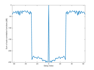
(a) The sum of auto-correlation functions, i.e., $|C_{x}(k)+C_{y}(k)|$.

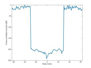
(b) The cross-correlation function, i.e., $|C_{xy}|(k)$

Figure 2: Two figures about the QOZCP $(\mathbf{x},\mathbf{y})$ by the Algorithm 1

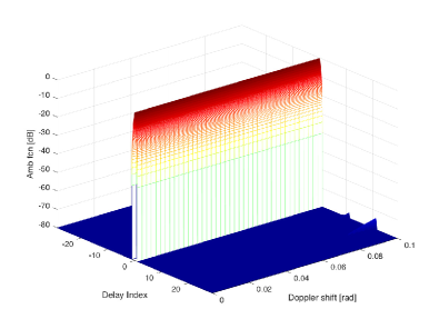
(a) The AAF of a DR-GCP sequence.

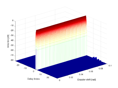
(b) The AAF of the a DR-QOZCP sequence

Figure 3: AAFs of the DR-GCP sequence and the DR-QOZCP sequence, respectively

Remark: For computing their AAF and CAF of DR-QOZCP sequence(s), $\mathbf{x}_{Q}$, $\mathbf{y}_{Q}$, and $\mathbf{x}_{G}$, $\mathbf{y}_{G}$ can be substituted into $\mathbf{x}$, $\mathbf{y}$ in (83) and (84).

Some conclusions can be drawn based on Table I, Table II, and Fig. 2 to Fig. 4.

• At first, we will compare $(L,Z)$-QOZCP ($\mathrm{PAPR}=5$) with length-$L$ GCP on maximun complementary sidelobe and cross correlation in delay interval $[-Z+1,Z-1]$. As Table I shows, there is a significant difference between QOZCP and GCP. Although QOZCP and GCP both have good complementary sidelobe in delay interval $[-Z+1,Z-1]$, QOZCP has much lower cross correlation than GCP in $[-Z+1,Z-1]$.

• As shown in Fig. 2, two figures about the obtained $(L,Z)$-QOZCP $(\mathbf{x},\mathbf{y})$ by SDAMM, where $L=64$,$Z=30$, $\mathrm{PAPR}=5$. Fig. 2(a) is the sum of correlation functions $C_{x}(k)+C_{y}(k)$ and Fig. 2(b) is the cross-correlation function $C_{xy}(k)$. The sidelobe in Fig. 2(a) is very low in delay interval $[-Z+1,Z-1]$. The cross-correlation level in interval $[-Z+1,Z-1]$ in Fig. 2(b) is also very low.

• Besides, we will compare DR-QOZCP with DR-GCP on Maximun Auto-Ambiguity Function Sidelobes in $\Omega_{1}$ and Maximun Cross-Ambiguity Function in $\Omega_{2}$ , where $\Omega_{1}=\{(k,\theta)|k\in[-Z+1,Z-1],\theta\in[0,0.1]\}$ and $\Omega_{2}=\{(k,\theta)|k\in[-Z+1,Z-1],\theta\in[0,3]\}$. What is interesting in table II is that DR-QOZCPs derived by $(L,Z)$-QOZCP have much lower Maximun Cross-Ambiguity Function than DR-GCPs’, while Maximun Auto-Ambiguity Function Sidelobes are low for both DR-GCP and DR-QOZCP.

• Fig. 3(a) and Fig. 3(b) show an AAF of the DR-GCP sequence and that of the DR-QOZCP sequence in the Delay interval $[-Z+1,Z-1]$ and Doppler interval $[0,0.1]$. The sidelobes of the designed sequence in delay interval $[-Z+1,Z-1]$ are almost as good as that of the DR-GCP sequence along any Doppler shift in $[0,0.1]$.

• Fig. 4(a) and Fig. 4(b) show an AAF of a DR-GCP sequence and that of the designed DR-QOZCP sequence, respectively, in the Delay interval $[-20,20]$ and Doppler interval $[0,3]$. The level of Fig. 4(b) is significantly lower than that of Fig. 4(a). For the system, the cross polarization aliasing is sufficiently vanished along any Doppler shift in $[0,3]$ when the proposed sequence pair is used.

In short, the Doppler resilient performance of our DR-QOZCP sequences is significantly better than that of DR-GCP sequences.

(a) The CAF of two DR-GCP sequences

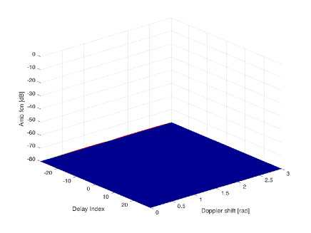
(b) The CAF of two DR-QOZCP sequences

Figure 4: CAFs of DR-GCP sequences and DR-QOZCP sequences, respectively

VI Concluding Remarks and Open Problems

In this paper we have given two contributions. Firstly, we have proposed new sets of sequence pairs called “Quasi-Orthogonal Z-Complementary Pairs” (QOZCPs). Secondly, we have applied the proposed QOZCPs to design Doppler resilient waveforms for polarimetric radar systems with are also dual orthogonal. We have also solved an optimization problem efficiently by proposing SADMM algorithm in MM framework, which eventually constructs the proposed QOZCPs of any length. Finally, we have compared the ambiguity plots of the proposed QOZCPs with the ambiguity plots of the existing DR-GCPs. The comparison shows that the proposed QOZCPs are more efficient as compared to DR-GCPs when CAF plots are considered.

Owing to the efficiency of the QOZCPs in application scenarios, the reader is invited to propose systematic constructions of QOZCPs and analyze the structural properties of these pairs.

Appendix A
Proof of Proposition 1

Proof:

Calculate

$$\begin{split}\sum_{k=-L+1}^{L-1}w_{k}|\mathbf{z^{H}A_{k}z}|^{2}&=\sum_{k=-L+1}^{L-1}w_{k}\text{vec}(\mathbf{Z})^{H}\text{vec}(\mathbf{A}_{k})\text{vec}(\mathbf{A}_{k})^{H}\text{vec}(\mathbf{Z})\\ &=\text{vec}(\mathbf{Z})^{H}\left[\sum_{k=-L+1}^{L-1}w_{k}\text{vec}(\mathbf{A}_{k})\text{vec}(\mathbf{A}_{k})^{H}\right]\text{vec}(\mathbf{Z}),\end{split}$$ (85)

$$\begin{split}&\sum_{k=-L+1}^{L-1}\tilde{w}_{k}|\mathbf{z^{H}B_{k}z}|^{2}=\text{vec}(\mathbf{Z})^{H}\left[\sum_{k=-L+1}^{L-1}\tilde{w}_{k}\text{vec}(\mathbf{B}_{k})\text{vec}(\mathbf{B}_{k})^{H}\right]\text{vec}(\mathbf{Z}).\end{split}$$ (86)

We set $J_{A}=\sum_{k=-L+1}^{L-1}w_{k}\text{vec}(\mathbf{A}_{k})\text{vec}(\mathbf{A}_{k})^{H}$, and $J_{B}=\sum_{k=-L+1}^{L-1}w_{k}\text{vec}(\mathbf{B}_{k})\text{vec}(\mathbf{B}_{k})^{H}$. Then, It is easy to verify that the objective of (12) can be transformed into that of (13) ∎

Appendix B
Proof of proposition 2

Proof:

The objective of (13) can be majorized by

$$\begin{split}&M_{f_{1}}(\mathbf{Z},\mathbf{Z}^{(t)})\\ &=\lambda_{\mathbf{J}}\text{vec}(\mathbf{Z})^{H}\text{vec}(\mathbf{Z})+2\text{Re}(\text{vec}(\mathbf{Z})^{H}(\mathbf{J}-\lambda_{\mathbf{J}}\mathbf{I})\text{vec}(Z^{(t)}))+\text{vec}(\mathbf{Z}^{(t)})^{H}(\lambda_{\mathbf{J}}\mathbf{I}-\mathbf{J})vec(Z^{(t)})\end{split}$$ (87)

The first term is equal to a constant $\lambda_{\mathbf{J}}L^{2}$, and the last term is also a constant obviously. Therefore, we ignore the both terms and only keep the second term, and the objective of (13) can be majorized by the second term. It is noted that the coefficient 2 cannot make any effect on the optimization, so we remove it. ∎

Appendix C
Proof of Theorem 1

Proof:

Calculate

$$J\text{vec}(\mathbf{A}_{k}) = (\alpha J_{A}+(1-\alpha)J_{B})\text{vec}(\mathbf{A}_{k})=\alpha J_{A}\text{vec}(\mathbf{A}_{k})$$ (88)

$$= \sum_{i=1-L}^{L-1}w_{i}\alpha\text{vec}(A_{i})\text{vec}(A_{i})^{H}\text{vec}(A_{k})$$ (89)

$$= w_{k}\alpha\text{vec}(A_{k})\text{vec}(A_{k})^{H}\text{vec}(A_{k})$$ (90)

$$= w_{k}\alpha(2N-2|k|)\text{vec}(A_{k}).$$ (91)

Therefore,

$$\lambda_{A}(k)=w_{k}\alpha(2N-2|k|).$$ (92)

Calculate

$$J\text{vec}(\mathbf{B}_{k}) = (J_{A}+J_{B})\text{vec}(\mathbf{B}_{k})=J_{B}\text{vec}(\mathbf{B}_{k})$$ (93)

$$= \sum_{i=1-L}^{L-1}w_{i}\alpha\text{vec}(B_{i})\text{vec}(B_{i})^{H}\text{vec}(B_{k})$$ (94)

$$= w_{k}\alpha\text{vec}(B_{k})\text{vec}(B_{k})^{H}\text{vec}(B_{k})$$ (95)

$$= w_{k}(1-\alpha)(N-|k|)\text{vec}(A_{k}).$$ (96)

Therefore,

$$\lambda_{B}(k)=w_{k}(1-\alpha)(N-|k|);$$ (97)

Because $\lambda_{A}(k)$ and $\lambda_{B}(k)$ are the eigenvalue of $\mathbf{J}$, then

$$\lambda_{\mathbf{J}}=\max_{k}\left\{\max\{\lambda_{A}(k),\lambda_{B}(k)\right\}|k=-L+1,\cdots,L-1\}.$$ (98)

∎

Appendix D
Proof of Proposition 3

Proof:

The main operations are in (99)

$$\begin{split}&\text{Re}\left\{\text{vec}(\mathbf{Z})^{H}(\mathbf{J}-\lambda_{\text{max}}(\mathbf{J})\mathbf{I})\text{vec}(\mathbf{Z}^{(t)})\right\}\\ &=\text{Re}\left\{\text{vec}(\mathbf{Z})^{H}\left(\alpha\sum_{k=-L+1}^{L-1}w_{k}\text{vec}(\mathbf{A}_{k})\text{vec}(\mathbf{A}_{k})^{H}\right.\right.\\ &\qquad\left.\left.+(1-\alpha)\sum_{k=-L+1}^{L-1}\tilde{w}_{k}\text{vec}(\mathbf{B}_{k})\text{vec}(\mathbf{B}_{k})^{H}-\lambda_{\mathbf{J}}\mathbf{I}\right)\cdot\text{vec}(\mathbf{Z}^{(t)})\right\}\\ &=\text{Re}\left\{\sum_{k=-L+1}^{L-1}\alpha w_{k}(\text{Tr}(\mathbf{A}_{k}\mathbf{Z})\text{Tr}(\mathbf{A}_{-k}\mathbf{Z}^{(t)}))\right.\\ &\left.\qquad+\sum_{k=-L+1}^{L-1}(1-\alpha)\tilde{w}_{k}(\text{Tr}(\mathbf{B}_{k}\mathbf{Z})\text{Tr}(\mathbf{B}_{-k}\mathbf{Z}^{(t)}))-\lambda_{\mathbf{J}}\text{Tr}(\mathbf{Z}^{(t)}\mathbf{Z})\right\}\\ &=\text{Re}\left\{\alpha\text{Tr}(\sum_{k=-L+1}^{L-1}w_{k}r_{-k}^{(l)}\mathbf{A}_{k}\mathbf{Z})+(1-\alpha)\text{Tr}(\sum_{k=-L+1}^{L-1}\tilde{w}_{k}c_{-k}^{(l)}\mathbf{B}_{k}\mathbf{Z}))-\lambda_{\mathbf{J}}\text{Tr}(\mathbf{Z}^{(t)}\mathbf{Z})\right\}\\ &=\text{Re}\left\{\alpha Tr(\mathbf{Q}_{r}\mathbf{Z})+(1-\alpha)Tr(\mathbf{Q}_{c}\mathbf{Z})-\lambda_{\text{max}}(\mathbf{J})\text{Tr}(\mathbf{Z}^{(t)}\mathbf{Z})\right\}\\ &=\text{Re}\left\{\mathbf{z}^{H}\left(\alpha\mathbf{Q}_{r}+(1-\alpha)\mathbf{Q}_{c}-\lambda_{max}(\mathbf{J})\mathbf{z}^{(t)}(\mathbf{z}^{(t)})^{H}\right)\mathbf{z}\right\}\\ &=\text{Re}\left\{\mathbf{z}^{H}\left(\mathbf{Q}-\lambda_{max}(\mathbf{J})\mathbf{z}^{(t)}(\mathbf{z}^{(t)})^{H}\right)\mathbf{z}\right\}\end{split}$$ (99)

where

$$\begin{split}&\mathbf{Q}_{r}=\sum_{k=-L+1}^{L-1}w_{k}r_{-k}^{(l)}\mathbf{A}_{k}=\begin{bmatrix}\sum_{k=-L+1}^{L-1}w_{k}r_{-k}^{(l)}\mathbf{U}_{k}&\mathbf{O}\\ \mathbf{O}&\sum_{k=-L+1}^{L-1}w_{k}r_{-k}^{(l)}\mathbf{U}_{k}\end{bmatrix},\end{split}$$ (100)

$$\begin{split}&\mathbf{Q}_{c}=\sum_{k=-L+1}^{L-1}\tilde{w}_{k}c_{-k}^{(l)}\mathbf{B}_{k}&=\begin{bmatrix}\mathbf{O}&\sum_{k=-L+1}^{L-1}w_{k}c_{-k}^{(l)}\mathbf{U}_{k}\\ \mathbf{O}&\mathbf{O}\end{bmatrix}\end{split}$$ (101)

$$\mathbf{Q}=\alpha\mathbf{Q}_{r}+(1-\alpha)\mathbf{Q}_{c}.$$ (102)

∎

Appendix E
Proof of theorem 2

Proof:

It is well known that FFT(IFFT) computed autocorrelation function is given by [39]

$$\begin{split}&[C_{x}^{(t)}(0),C_{x}^{(t)}(1),\cdots,C_{x}^{(t)}(L-1),0,C_{x}^{(t)}(1-L),\cdots,C_{x}^{(t)}(-1)]^{T}=\mathbf{F}^{H}\!|\mathbf{F}[(\mathbf{y}^{(t)})^{T}\!,\mathbf{0}_{1\times L}]^{T}|^{2}.\end{split}$$ (103)

Similarly,

$$\begin{split}&[C_{y}^{(t)}(0),C_{y}^{(t)}(1),\cdots,C_{y}^{(t)}(L-1),0,C_{y}^{(t)}(1-L),\cdots,C_{y}^{(t)}(-1)]^{T}=\mathbf{F}^{H}\!|\mathbf{F}[(\mathbf{y}^{(t)})^{T}\!,\mathbf{0}_{1\times L}]^{T}|^{2}\end{split}$$ (104)

Also, $r_{k}^{(t)}=C_{x}^{(t)}(k)+C_{y}^{(t)}(k)$ holds, then the following equation is obviously obtained.

$$\begin{split}&\mathbf{r}=[r_{0}^{(t)},r_{1}^{(t)},\cdots,r_{L-1}^{(t)},0,r_{1-L}^{(t)},\cdots,r_{-1}^{(t)},]\\ &=\mathbf{F}^{H}\!|\mathbf{F}[(\mathbf{x}^{(t)})^{T}\!,\mathbf{0}_{1\times L}]^{T}|^{2}\!+\mathbf{F}^{H}\!|\mathbf{F}[(\mathbf{y}^{(t)})^{T}\!,\mathbf{0}_{1\times L}]^{T}|^{2}.\end{split}$$ (105)

The discrete Fourier transform of $x$ and $y$ can be written as

$$\sum_{l=1}^{L}x(l)e^{-j2\pi\omega_{i}l/L}\,\,\mathrm{and}\,\,\sum_{m=1}^{L}y(l)e^{-j2\pi\omega_{i}m/L},$$ (106)

respectively. It is easy to verify the following equation holds

$$\begin{split}&(\sum_{l=1}^{L}x(l)e^{-j2\pi\omega_{i}l/L})^{*}(\sum_{m=1}^{L}y(l)e^{-j2\pi\omega_{i}m/L})=\sum_{l=1}^{L}\sum_{m=1}^{L}x^{*}(l)y(m)e^{-j2\pi\omega_{i}m/L}\\ &=\sum_{k=-L+1}^{L-1}\sum_{l=0}^{L-1}x^{*}(l)y(k+l)e^{-j2\pi\omega_{i}k/L}=\sum_{k=-L+1}^{L-1}c_{k}e^{-j2\pi\omega_{i}k/L}\end{split}$$ (107)

where $k$ in second equation is to let $k=m-l$. Then it is easy to know the cross correlation $c_{k}=C_{xy}(k)$ can be obtained by inverse Fourier transform.

∎

Appendix F
Proof of Proposition 5

Proof:

The objective of (24) can be majorized by

$$\begin{split}&M_{f_{2}}(\mathbf{z},\mathbf{z}^{(t)})=\lambda_{u}\mathbf{z}^{H}\mathbf{z}+2\text{Re}(\mathbf{z}^{H}(\hat{\mathbf{Q}}-\lambda_{u}\mathbf{I})\mathbf{z}^{(t)})+(\mathbf{z}^{(t)})^{H}(\lambda_{u}\mathbf{I}-\mathbf{J})\mathbf{z}^{(t)}\end{split}$$ (108)

where $\hat{\mathbf{Q}}=\mathbf{Q}+\mathbf{Q}^{H}-2\lambda_{\mathbf{J}}\mathbf{z}^{(t)}(\mathbf{z}^{(t)})^{H}$. Similarly,

Since $\lambda_{u}$ should be larger than $\lambda_{max}(\hat{\mathbf{Q}})$, and $\lambda_{max}(\mathbf{Q}+\mathbf{Q}^{H})$ is larger than $\lambda_{max}(\hat{\mathbf{Q}})$, then we can let $\lambda_{u}>\lambda_{max}(\mathbf{Q}+\mathbf{Q}^{H})$ so that $\lambda_{u}>\lambda_{max}(\hat{\mathbf{Q}})$.

Based on the fact in [26], the following inequality holds

$$\lambda_{max}(\mathbf{Q}+\mathbf{Q}^{H})\leq 2L\max|a_{ij}|,\quad i,j\in\{1,2,\cdots,2L\}$$ (109)

where $a_{ij}$ is the elements of the matrix $\mathbf{Q}+\mathbf{Q}^{H}$. Besides, the following inequality holds

$$2\max|Q_{ij}|\geq\max|Q_{ij}|+\max|Q_{ji}^{*}|\geq\max|a_{ij}|,$$

and we have $4L(\max\limits_{1\leq i,j\leq L}|Q_{i,j}|)>2L\max|a_{ij}|$, where $Q_{ij}$ is the elements of $\mathbf{Q}$.

Hence, $\lambda_{u}=4L(\max\limits_{1\leq i,j\leq L}|\mathbf{Q}_{i,j}|)$ ∎

Appendix G
for calculating $x=\mathrm{proj}_{0}(\cdot)$

Let

$$x_{k}^{(t+1)}=|x_{k}^{(t+1)}|e^{j\,\mathrm{arg}(\mathbf{P}_{x}(\mathbf{z}^{(t)}))}$$

• if $mp_{c}^{2}\leq p_{e}$,

  $$\left|x_{k}^{(t+1)}\right|=\left\{\begin{array}[]{ll}{p_{c}}&{k=1,\cdots,m}\\ {\sqrt{\frac{p_{e}-mp_{c}^{2}}{p_{e}-m}}}&{k=m+1,\cdots,L}\end{array}\right.$$

• else if $mp_{c}^{2}>p_{e}$

  $$\left|x_{k}^{(t+1)}\right|=\min\left\{\delta\left|v_{k}^{(t)}\right|,\gamma\right\}$$

  where $\delta\in\left[0,\frac{\gamma}{\min\left\{\left|v_{k}^{(t)}\right|,\left|v_{k}^{(t)}\right|\neq 0\right\}}\right]$ can be obtained by solving the following equation by bisection method.

  $$\sum_{n=1}^{N}\min\left\{\delta^{2}\left|v_{k}^{(t)}\right|^{2},\gamma^{2}\right\}=p_{e}.$$ (110)

References

• [1] M. J. Golay, “Static multislit spectrometry and its application to the panoramic display of infrared spectra,” JOSA, vol. 41, no. 7, pp. 468–472, 1951.
• [2] M. Golay, “Complementary series,” IRE Trans. Inf. Theory, vol. 7, no. 2, pp. 82–87, 1961.
• [3] P. B. Borwein and R. A. Ferguson, “A complete description of Golay pairs for lengths up to 100,” Mathematics of computation, vol. 73, pp. 967–985, Jul. 2003.
• [4] J. A. Davis and J. Jedwab, “Peak-to-mean power control in OFDM, Golay complementary sequences, and Reed-Muller codes,” IEEE Trans. Inf. Theory, vol. 45, no. 7, pp. 2397–2417, Nov. 1999. doi: 10.1109/18.796380
• [5] K. Feng, P. Jau-Shyong, and Q. Xiang, “On aperiodic and periodic complementary binary sequences,” IEEE Trans. Inf. Theory, vol. 45, no. 1, pp. 296–303, Jan. 1999.
• [6] P. Fan, W. Yuan, and Y. Tu, “Z-complementary binary sequences,” IEEE Signal Process. Lett., vol. 14, no. 8, pp. 509–512, Aug. 2007.
• [7] Z. Liu, U. Parampalli, and Y. L. Guan, “On even-period binary Z-complementary pairs with large ZCZs,” IEEE Signal Process. Lett., vol. 21, pp. 284–287, 2014.
• [8] A. R. Adhikary, S. Majhi, Z. Liu, and Y. L. Guan, “New sets of optimal odd-length binary Z-complementary pairs,” IEEE Trans. Inf. Theory, vol. 66, pp. 669–678, 2020.
• [9] A. R. Adhikary, P. Sarkar, and S. Majhi, “A direct construction of $q$-ary even length Z-complementary pairs using generalized Boolean functions,” IEEE Signal Process. Lett., vol. 27, pp. 146–150, 2020.
• [10] C.-Y. Chen, “A novel construction of Z-complementary pairs based on generalized boolean functions,” IEEE Signal Process. Lett., vol. 24, pp. 987–990, 2017.
• [11] B. Shen, Y. Yang, Z. Zhou, P. Fan, and Y. Guan, “New optimal binary Z-complementary pairs of odd length $2^{m}+3$,” IEEE Signal Process. Lett., vol. 26, pp. 1931–1934, 2019.
• [12] Z. Gu, Y. Yang, and Z. Zhou, “New sets of even-length binary Z-complementary pairs,” in 2019 Ninth International Workshop on Signal Des. App. Commun. (IWSDA).   IEEE, 2019, pp. 1–5.
• [13] G. Gong, F. Huo, and Y. Yang, “Large zero autocorrelation zones of Golay sequences and their applications,” vol. 61, pp. 3967–3979, 2013.
• [14] C.-Y. Chen and S.-W. Wu, “Golay complementary sequence sets with large zero correlation zones,” IEEE Trans. Commun., vol. 66, pp. 5197–5204, 2018.
• [15] C. D. Groot, D. Würtz, and K. Hoffmann, “Low autocorrelation binary sequences: exact enumeration and optimization by evolutionary strategies,” Optimization, vol. 23, no. 4, pp. 369–384, 1992.
• [16] P. Stoica, H. He, and J. Li, “New algorithms for designing unimodular sequences with good correlation properties,” IEEE Trans. Signal Process., vol. 57, no. 4, pp. 1415–1425, 2009.
• [17] ——, “On designing sequences with impulse-like periodic correlation,” IEEE Signal Process. Lett., vol. 16, pp. 703–706, 2009.
• [18] W. Rowe, P. Stoica, and J. Li, “Spectrally constrained waveform design,” IEEE Signal Process. Mag., vol. 31, pp. 157–162, 2014.
• [19] M. Soltanalian, M. M. Naghsh, and P. Stoica, “A fast algorithm for designing complementary sets of sequences,” Signal Processing, vol. 93, no. 7, pp. 2096–2102, 2013.
• [20] M. Soltanalian and P. Stoica, “Computational design of sequences with good correlation properties,” IEEE Trans. Signal Process., vol. 60, pp. 2180–2193, 2012.
• [21] F.-C. Li, Y.-N. Zhao, and X.-L. Qiao, “A waveform design method for suppressing range sidelobes in desired intervals,” Signal Processing, vol. 96, pp. 203–211, 2014.
• [22] J. Zhang, X. Qiu, C. Shi, and Y. Wu, “Cognitive radar ambiguity function optimization for unimodular sequence,” EURASIP J. Adv Signal Process., vol. 2016, no. 1, p. 31, 2016.
• [23] F. Arlery, R. Kassab, U. Tan, and F. Lehmann, “Efficient gradient method for locally optimizing the periodic/aperiodic ambiguity function,” in Radar Conference (RadarConf), 2016 IEEE.   IEEE, 2016, pp. 1–6.
• [24] ——, “Efficient optimization of the ambiguity functions of multi-static radar waveforms,” in Radar Symposium (IRS), 2016 17th International.   IEEE, 2016, pp. 1–6.
• [25] U. Tan, C. Adnet, O. Rabaste, F. Arlery, J.-P. Ovarlez, and J.-P. Guyvarch, “Phase code optimization for coherent mimo radar via a gradient descent,” in 2016 IEEE Radar Conference (RadarConf).   IEEE, 2016, pp. 1–6.
• [26] J. Song, P. Babu, and D. P. Palomar, “Optimization methods for designing sequences with low autocorrelation sidelobes,” IEEE Trans. Signal Process., vol. 63, no. 15, pp. 3998–4009, 2015.
• [27] J. Liang, H. C. So, J. Li, and A. Farina, “Unimodular sequence design based on alternating direction method of multipliers,” IEEE Trans. Signal Process., vol. 64, no. 20, pp. 5367–5381, 2016.
• [28] A. R. Calderbank, S. D. Howard, W. Moran, A. Pezeshki, and M. Zoltowski, “Instantaneous radar polarimetry with multiple dually-polarized antennas,” in Conf. Rec. 40th Asilomar Conf. Signals, Systemas and Computers.   Pacific Grove, CA, Oct. 2006, pp. 757–761.
• [29] A. Pezeshki, A. R. Calderbank, W. Moran, and S. D. Howard, “Doppler resilient Golay complementary waveforms,” IEEE Trans. Inf. Theory, vol. 54, no. 9, pp. 4254–4266, Sep. 2008.
• [30] Y. Cui, X. Gao, and R. Li, “Broadband vertically/horizontally dual-polarized antenna for base stations,” Int. J. Antennas and Propagation, vol. 2017, Mar. 2017.
• [31] S. D. Howard, A. R. Calderbank, and W. Moran, “A simple signal processing architecture for instantaneous radar polarimetry,” IEEE Trans. Inf. Theory, vol. 53, no. 4, pp. 1282–1289, Apr. 2007.
• [32] S. Searle and S. Howard, “A novel polyphase code for sidelobe suppression,” in 2007 Int Waveform Diversity Des. Conf., 2007, pp. 377–381.
• [33] S. J. Searle and S. D. Howard, “A novel nonlinear techique for sidelobe suppression in radar,” in 2007 IET Int. Conf. Radar Systems, 2007, pp. 1–5.
• [34] K. Harman and B. Hodgins, “The next generation of GUIDAR technology,” in 38th Annual Int. Carnahan Conf. Security Technology, 2004., 2004, pp. 169–176.
• [35] J. Tang, N. Zhang, Z. Ma, and B. Tang, “Construction of Doppler resilient complete complementary code in mimo radar,” IEEE Trans. Signal Process., vol. 62, no. 18, pp. 4704–4712, 2014.
• [36] J. Wang, P. Fan, Y. Yang, Z. Liu, and Y. L. Guan, “Doppler resilient Z-complementary waveforms from ESP sequences,” in 2017 Eighth International Workshop on Signal Des. App. Commun. (IWSDA).   IEEE, 2017, pp. 19–23.
• [37] D. Giuli, M. Fossi, and L. Facheris, “Radar target scattering matrix measurement through orthogonal signals,” IEE Proc. F - Radar and Signal Process., vol. 140, no. 4, pp. 233–242, 1993.
• [38] C. Titin-Schnaider and S. Attia, “Calibration of the meric full-polarimetric radar: theory and implementation,” Aerospace Sc. and Tech., vol. 7, no. 8, pp. 633 – 640, 2003.
• [39] J. Song, P. Babu, and D. P. Palomar, “Sequence design to minimize the weighted integrated and peak sidelobe levels,” IEEE Trans. Signal Process., vol. 64, no. 8, pp. 2051–2064, Apr. 2016.
• [40] L. Zhao, J. Song, P. Babu, and D. P. Palomar, “A unified framework for low autocorrelation sequence design via majorization–minimization,” IEEE Trans. Signal Process., vol. 65, no. 2, pp. 438–453, 2016.
• [41] Y. Wang, Y. Wang, and Q. Shi, “Optimized signal distortion for PAPR reduction of OFDM signals with IFFT/FFT complexity via ADMM approaches,” IEEE Trans. Signal Process., vol. 67, no. 2, pp. 399–414, Jan. 2019.
• [42] J. A. Tropp, I. S. Dhillon, R. W. Heath, and T. Strohmer, “Designing structured tight frames via an alternating projection method,” IEEE Trans. Inf. Theory, vol. 51, no. 1, pp. 188–209, 2005.
• [43] M. Soltanalian and P. Stoica, “Designing unimodular codes via quadratic optimization.” IEEE Trans. Signal Process., vol. 62, no. 5, pp. 1221–1234, 2014.
• [44] J. Yang, G. Cui, X. Yu, Y. Xiao, and L. Kong, “Cognitive local ambiguity function shaping with spectral coexistence,” IEEE Access, vol. 6, pp. 50 077–50 086, 2018.