The LOFAR view of intergalactic magnetic fields
with giant radio galaxies

Abstract

Context. Giant radio galaxies (GRGs) are physically large radio sources that extend well beyond their host galaxy environment. Their polarization properties are affected by the poorly constrained magnetic field that permeates the intergalactic medium on Mpc scales. A low frequency (¡ 200 MHz) polarization study of this class of radio sources is now possible with LOFAR.

Aims. Here we investigate the polarization properties and Faraday rotation measure (RM) of a catalog of GRGs detected in the LOFAR Two-metre Sky Survey. This is the first low frequency polarization study of a large sample of radio galaxies selected on their physical size. We explore the magneto-ionic properties of their under-dense environment and probe intergalactic magnetic fields using the Faraday rotation properties of their radio lobes. LOFAR is a key instrument for this kind of analysis because it can probe small amounts of Faraday dispersion ($<$ 1 rad m^-2) which are associated with weak magnetic fields and low thermal gas densities.

Methods. We use RM synthesis in the 120-168 MHz band to search for polarized emission and to derive the RM and fractional polarization of each detected source component. We study the depolarization between 1.4 GHz and 144 MHz using images from the NRAO VLA Sky Survey. We investigate the correlation of the detection rate, the RM difference between the lobes and the depolarization with different parameters: the angular and linear size of the sources and the projected distance from the closest foreground galaxy cluster. We included in our sample also 3C 236, one of the largest radio galaxies known.

Results. From a sample of 240 GRGs, we detected 37 sources in polarization, all with a total flux density above 56 mJy. We detected significant RM differences between the lobes which would be inaccessible at GHz frequencies, with a median value of $\sim$1 rad m^-2. The fractional polarization of the detected GRGs at 1.4 GHz and 144 MHz is consistent with a small amount of Faraday depolarization (a Faraday dispersion $<0.3$ rad m^-2). Our analysis shows that the lobes are expanding into a low-density (¡10^-5 cm^-3) local environment permeated by weak magnetic fields (¡0.1 $\mu$G) with fluctuations on scales of 3 to 25 kpc. The presence of foreground galaxy clusters appears to influence the polarization detection rate up to 2R₅₀₀. In general, this work demonstrates the ability of LOFAR to quantify the rarefied environments in which these GRGs exist and highlights them as an excellent statistical sample to use as high precision probes of magnetic fields in the intergalactic medium and the Milky Way.

1 Introduction

Radio galaxies that extend to Mpc scales are often defined as giant radio galaxies (GRGs, Willis et al., 1974). While earlier authors adopted a lower limit of 1 Mpc to define GRGs assuming $H_{0}$ = 50 km s^-1, nowadays the general consensus is to use a limiting size of 0.7 Mpc in order to maintain the classification within the revised cosmology (e.g., Dabhade et al., 2017; Kuźmicz et al., 2018). GRGs are mostly Fanaroff-Riley type 2 radio galaxies (FR II, Fanaroff & Riley, 1974), with the lobes extending well beyond the host galaxy and local environment, and expanding into the surrounding intergalactic medium (IGM). They are particularly interesting objects for the study of different astrophysical problems, ranging from the evolution of radio sources (Ishwara-Chandra & Saikia, 1999) to the ambient gas density (Mack et al., 1998; Malarecki et al., 2015; Subrahmanyan et al., 2008). In particular, Faraday rotation and polarization properties of the lobes/hotspots emission can be used to study the nature of the intergalactic magnetic field (IGMF, O’Sullivan et al., 2019). In the future, giant radio galaxies will also be targeted with the Square Kilometre Array (SKA) to probe the warm-hot intergalactic medium (WHIM, Peng et al., 2015).

GRGs are a small subclass of radio galaxies: they constitute about $6\ \%$ of the complete sample of 3CR radio sources (Laing et al., 1983). Until recently only a few hundred GRGs have been reported (e.g., Kuźmicz et al., 2018, and references therein). The LOFAR Two-metre Sky Survey (LoTSS, Shimwell et al., 2017, 2019) is one of the best surveys to identify GRGs thanks to its high sensitivity to low surface brightness sources, the high angular resolution, and the high quality associations with optical counterparts including redshifts. Recently, Dabhade et al. (2020) reported a large catalog of 239 GRGs, of which 225 were new findings from the LoTSS first data release (DR1). Optical/infrared identifications and redshift estimates are available for all the sample (Williams et al., 2019; Duncan et al., 2019).

Polarization observations in the 120-168 MHz band provide exceptional Faraday rotation measure (RM) accuracy due to the large wavelength-square coverage (Brentjens, 2018; Van Eck, 2018). Despite the technical challenges, preliminary efforts to build a polarization catalog with LOFAR were successfully performed (Mulcahy et al., 2014; Van Eck et al., 2018; Neld et al., 2018). LOFAR polarization capabilities have been recently shown to be well suited for the study of magnetic fields for different science cases: from the interstellar medium (Van Eck et al., 2019) to the cosmic web (O’Sullivan et al., 2019, 2020). However, at these low frequencies most of the sources remain undetected in polarization, largely because of Faraday depolarization effects (Burn, 1966; Farnsworth et al., 2011). Depolarization is less severe in low-density ionised environments characterized by weak magnetic fields with large fluctuation scales (compared to the resolution of the observations), since it depends on the magnetic field and thermal electron density along the line of sight, and on their spatial gradient within the synthesized beam.

Previous work probed the strong polarization of the lobes of GRGs at low frequencies (e.g., Willis et al., 1978a; Bridle et al., 1979; Tsien, 1982; Mack et al., 1997). One of the first objects observed in polarization by LOFAR was the double-double giant radio galaxy B1834+620 (Orrù et al., 2015) and, recently, a polarization study of the giant radio galaxy NGC 6251 was performed with LOFAR (Cantwell et al. 2020, submitted). Machalski & Jamrozy (2006) also showed that GRGs are less depolarized at 1.4 GHz than normal-sized radio galaxies, indicating the presence of less dense gas surrounding their lobes. Hence, the lobes of GRGs are probably one of the best targets for polarization studies at low frequencies (O’Sullivan et al., 2018a). While previous GRGs polarization studies were based on single sources, or at most tens of objects, observed with different facilities, LOFAR allows us to perform the first study on a large sample of hundreds of GRGs that were selected and analyzed consistently.

A low density ($\sim 10^{-5}-10^{-6}$ cm^-3) WHIM permeate the large scale structure of the Universe, from the extreme outskirts of galaxy clusters to filaments (Davé et al., 2001). Previous studies demonstrated that lobes of GRGs evolve and interact with the WHIM (Mack et al., 1998; Chen et al., 2011). In these regions, the IGMF is expected to range from 1 to 100 nG, with the true value being important to discriminate between different magneto-genesis scenarios (Brüggen et al., 2005; Vazza et al., 2017; Vernstrom et al., 2019). While the detection of both thermal and non-thermal emission of the WHIM is still an observational challenge (Vazza et al., 2019), GRGs are potentially indirect probes of these poorly constrained regions of the Universe (Subrahmanyan et al., 2008). RM and depolarization information derived from polarized emission of GRGs can yield tomographic information about this extremely rarefied environment (O’Sullivan et al., 2019).

While in this work GRGs are mainly exploited for the study of the IGM, the polarization properties of radio galaxies, in general, are crucial for the study of magnetic field structures in lobes and jets. A preliminary census of polarized sources in the LoTSS field was performed by Van Eck et al. (2018). They produced a catalog of 92 point-like sources with a resolution of $4.3\arcmin$ and a sensitivity of 1 mJy/beam within a region of 570 deg². O’Sullivan et al. (2018a) analyzed 76 out of the 92 sources residing in the DR1 area with an improved resolution of $20\arcsec$ and O’Sullivan et al. (2019) performed a detailed study of the largest radio galaxy in the sample. A complete statistical study of the bulk polarization properties of radio galaxies in the LoTSS DR1 will be presented in Mahatma et al. (2020, in prep.). The aim of our study based on the selection of radio galaxies with large physical size is twofold: on one hand it allows us to complement the work by Dabhade et al. (2020) with polarization information on the GRG sample, and, on the other hand, this selection is particularly interesting for the study of IGMF. Small size radio galaxies would be more affected by the host galaxy halo and local environment than GRGs and the detection rate would be strongly reduced by the Faraday depolarization.

Recently, O’Sullivan et al. (2020) presented a study of the magnetization properties of the cosmic web comparing the RM difference between lobes of radio galaxies (i.e., physical pairs) and pairs of physically unrelated sources. This work made use of the exceptional RM accuracy of LOFAR and applied the same strategy that Vernstrom et al. (2019) implemented to analyze the data at 1.4 GHz of the NRAO VLA Sky Survey (NVSS, Condon et al., 1998). The difference in the results obtained by these works is attributed mainly to the Faraday depolarization which made the higher RM variance, detected by the NVSS, undetectable by LOFAR. Here, we can deeply investigate the origin of such depolarization on a well defined sample of sources.

In this paper, we present a polarization and RM analysis of the GRGs detected in the LoTSS DR1 (Dabhade et al., 2020), plus one of the largest radio galaxies (3C 236) observed with LOFAR as part of the ongoing LoTSS (Shulevski et al., 2019). The specific nature of the sample analyzed here is that all sources have a physical size larger than 0.7 Mpc. In Sec. 2, we describe the data reduction, polarization and Faraday rotation analysis, the source identification, and the depolarization study. In Sec. 3 we present the main properties of the detected sources and we investigate the origins of Faraday rotation and depolarization. In Sec. 4 we discuss the results and their implications for the study of the IGMF. We conclude with a summary in Sec. 5. The images of all the detected sources are shown in Appendix A. Throughout this paper, we assume a $\Lambda$CDM cosmological model, with $H_{0}$ = 67.8 km s^-1 Mpc^-1, $\Omega_{\rm M}$ = 0.308, $\Omega_{\Lambda}$ = 0.692 (Planck Collaboration et al., 2016).

2 Data analysis

Our work is based on the data from the LoTSS, fully described by Shimwell et al. (2017, 2019). This ongoing survey is covering the entire northern sky with the LOFAR High-Band Antenna (HBA) at frequencies from 120 to 168 MHz. The LoTSS DR1 consists of images at 6$\arcsec$ resolution and a sensitivity of $\sim$70 $\mu$Jy/beam. It covers 424 deg² in the region of the HETDEX Spring field (i.e., 2$\%$ of the northern sky). The observing time for each pointing is $\sim$8 hours and the FWHM of the primary beam is $\sim 4^{\circ}$. Although our work is mainly based on the GRG catalog by Dabhade et al. (2020) which is located in the DR1 region, we make use of the updated data products from the upcoming LoTSS second data release (DR2).

2.1 Calibration and Data Reduction

We refer the reader to Shimwell et al. (2017) for the full details on the calibration and data reduction. Here we summarize only the main steps.

For our analysis we used images at 20$\arcsec$ and 45$\arcsec$ resolution. The choice of a restoring beam larger than $6\arcsec$ (used for the LoTSS DR1) was meant to maximize the sensitivity to the extended emission of the lobes. The 20$\arcsec$ resolution images from the upcoming LoTSS DR2 pipeline (Tasse et al. 2020, in prep.) were used to identify polarized sources and record the position, polarized flux density, fractional polarization, and RM of the pixels with the highest signal-to-noise ratio (see Sec. 2.3). The $45\arcsec$ resolution images of the detected sources were instead necessary to compare with images at 1.4 GHz and perform the depolarization analysis (see Sec. 2.4). We used two different strategies for calibration and imaging at the two resolutions to cross-check the reliability from the ddf-pipeline (Tasse, 2014; Tasse et al., 2018; Shimwell et al., 2019) output and also to enable deconvolution in Stokes $Q$ and $U$ at 45$\arcsec$. We obtained reliable calibration and imaging performance with both procedures, described in the following.

Direction-dependent calibration was performed using the ddf-pipeline. Direction-dependent calibrated data were used for the total intensity images at 20$\arcsec$ resolution in order to better resolve the morphological properties of the sources. These data were also used to image Stokes $Q$ and $U$ frequency channel cubes at 20$\arcsec$ resolution.

We made low resolution 45$\arcsec$ images of the GRGs that were detected in polarization at 20$\arcsec$ (see Sec. 2.3). Only direction-independent calibration was performed using PREFACTOR 1.0 (van Weeren et al., 2016; Williams et al., 2016). This procedure is robust, because of the absence of any large direction-dependent artifacts in the Q and U images, and allows us to deconvolve the emission at $45\arcsec$ without re-running the entire calibration on the full LoTSS field where a GRG has been detected. The rms noise level was on average one order of magnitude larger at $45\arcsec$ than at $20\arcsec$ due to uv-cut and down-weighting of data on the longer baselines. The direction-independent calibrated data were phase-shifted to the source location and averaged to 40 s (from 8 s) to speed up the imaging and deconvolution process (as in, e.g., Neld et al., 2018; O’Sullivan et al., 2019).

The ionospheric RM correction was applied with RMextract (Mevius, 2018). Residual ionospheric RM correction errors are estimated to be $\sim 0.05$ rad m^-2 between observations and $\sim 0.1-0.3$ rad m^-2 across the 8h observations (Sotomayor-Beltran et al., 2013; Van Eck et al., 2018).

2.2 Polarization and Faraday rotation imaging

The $Q$ and $U$ images at $20\arcsec$ resolution were not deconvolved because this procedure is not yet implemented in the ddf-pipeline. Although some of the RM structure for the brightest polarized sources is dominated by spurious structure, this should not affect our analysis since we used the RM value at the peak of the polarized emission. We used WSCLEAN 2.4 (Offringa et al., 2014) to deconvolve the $Q$ and $U$ images at 45$\arcsec$ resolution, in order to directly compare with polarization images from the NVSS at 1.4 GHz (Condon et al., 1998). In $90\ \%$ of the cases, we obtained consistent RMs at $45\arcsec$ and $20\arcsec$. We found a larger scatter in the values obtained at low resolution, as expected due to the larger beam and higher noise.

We created 480 $Q$ and $U$ frequency channel images with 0.1 MHz resolution between 120 and 168 MHz with a fixed restoring beam (20$\arcsec$ or 45$\arcsec$). The primary beam correction was applied to each channel. The total intensity ($I$) image was created using the entire band at the central frequency of 144 MHz and then corrected for the primary beam. All pixels below 1 mJy/beam in total intensity (for which no fractional polarization $<50\ \%$ can be detected due to the LoTSS sensitivity) were masked out to speed up the subsequent analysis.

We performed RM synthesis (Brentjens & de Bruyn, 2005) on the $Q$ and $U$ per-channel cubes using PYRMSYNTH to obtain the cubes in the Faraday depth ($\phi$) space. In these cubes every pixel contains the Faraday spectrum along the line of sight, i.e., the polarized intensity at each Faraday depth (see, e.g., Stuardi et al., 2019, for the used terminology). An example Faraday spectrum extracted from the peak of polarized intensity of a source is shown in Fig. 1. RM clean was also performed on the $45\arcsec$ cubes (Heald, 2009).

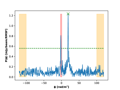
Figure 1: Example Faraday spectrum. In particular, this is the Faraday spectrum obtained at the polarized peak position of the lobe “b” of GRG 2 (see Tab. 7). The red shadowed area shows the region of the spectrum excluded due to the instrumental leakage contamination. The orange areas show the range used to compute the rms noise from the $Q$ and $U$ Faraday spectra. The green dashed line highlights the 8$\sigma$ detection threshold. The green “X” marks the position of the peak from which we derived the RM and $P$ values of the pixel.

Considering the LoTSS bandwidth and the adopted channelization, using Brentjens & de Bruyn (2005) we can estimate our resolution in Faraday space, $\delta\phi$ = 1.16 rad m^-2, the maximum observable Faraday depth, $|\phi_{\rm max}|$ = 168 rad m^-2, and the largest observable scale in Faraday space, $\Delta\phi_{\rm max}$ = 0.97 rad m^-2. As a consequence, with the LoTSS we can detect only emission that is unresolved in Faraday depth. Faraday cubes were created between -120 and 120 rad m^-2 and sampled at 0.3 rad m^-2. The Faraday range was chosen considering that RM values for sources at high Galactic latitude (above $b>55^{\circ}$) and outside galaxy cluster environments are a few tens of rad m^-2 (see, e.g., Böhringer et al., 2016).

The LOFAR calibration software (i.e. PREFACTOR 1.0) does not allow instrumental polarization leakage correction so that peaks appear in the Faraday spectrum at the level of $\sim 1.5\ \%$ of the total intensity in the range $-3<\phi<1$ rad m^-2 (see Fig. 1). This asymmetric range is due to the ionospheric RM correction that shifts the leakage peak along the Faraday spectrum (Van Eck et al., 2018). We thus excluded this range in order to avoid a contamination from the instrumental leakage as done by other authors (e.g., Neld et al., 2018; O’Sullivan et al., 2019). This method systematically excludes from this analysis all real polarized sources within this Faraday depth range. We fitted pixel-by-pixel a parabola around the main peak of the Faraday spectrum outside the excluded range. We obtained the RM and polarized intensity ($P$) images from the position of the parabola vertex in each pixel. For each pixel we computed the noise, $\sigma_{QU}$, as the standard deviation in the outer $20\ \%$ of the $Q$ and $U$ Faraday spectra and we imposed an initial 6$\sigma_{QU}$ detection threshold, which ensures an equivalent 5$\sigma$ Gaussian significance (Hales et al., 2012). We also computed the fractional polarization ($p$) images by dividing the polarization image $P$ obtained from the RM-synthesis by the full-band total intensity image $I$ (with a 3$\sigma$ detection threshold, where $\sigma$ is the local rms noise). We computed the fractional polarization error map by propagating the uncertainties on $P$ and $I$ images.

The RM error map was computed as $\delta\phi$ divided by twice the signal-to-noise of the detection (Brentjens & de Bruyn, 2005). This formula is computed for zero spectral index and equal rms noise in Stokes $Q$ and $U$ and it can be used as a reference value. Furthermore, the computed error does not include the systematic error from the ionospheric RM correction ($\sim$0.1 rad m^-2, Van Eck et al., 2018).

2.3 Source identification

Table 1: Polarized GRGs.

GRG	R.A.	Dec	$z$	Ang. size	Lin. size	FR	Remark
	(deg)	(deg)		(arcsec)	(Mpc)
1	164.273	53.440	0.460	153	0.92	II	d
2	164.289	48.678	0.276	439	1.9	II	d
7	164.575	51.672	0.415	330	1.86	II	s
19	167.402	53.230	0.288	230	1.03	II	d
22	168.381	46.371	0.589	112	0.76	II	d
44	174.882	47.357	0.518	312	2.0	II	s
47	178.000	49.849	0.891	96	0.77	II	s
51	180.345	49.427	0.205	345	1.2	I	d
57	182.692	53.490	0.448	119	0.71	I	s
64	184.576	53.456	0.568	183	1.23	II	d
65	184.708	50.438	0.199	210	0.71	II	d
77	186.493	53.161	0.811	147	1.14	II	d
80	187.498	53.546	0.523	137	0.88	II	s
83	188.210	49.107	0.690	256	1.87	II	s
85	188.756	53.299	0.345	683	3.44	II	d
87	189.202	46.068	0.615	125	0.87	II	d
91	190.052	53.577	0.293	164	0.74	II	d
103	195.396	54.136	0.313	168	0.79	II	d
112	197.620	52.228	0.650	197	1.41	II	s
117	199.144	49.544	0.563	126	0.84	II	core
120	200.124	49.280	0.684	113	0.82	II	d
122	200.902	47.497	0.440	180	1.05	II	s
136	203.345	53.547	0.354	173	0.88	-	s
137	203.549	55.024	1.245	91	0.78	II	s
144	204.845	50.963	0.316	174	0.83	II	d
145	205.263	49.267	0.747	113	0.85	II	d
148	206.065	48.764	0.725	202	1.51	II	s
149	206.174	50.383	0.763	123	0.93	II	s
165	210.731	51.458	0.518	135	0.87	II	d
166	210.813	51.746	0.485	228	1.41	II	d
168	211.421	54.182	0.761	116	0.88	II	d
177	213.535	48.699	1.361	107	0.92	II	d
207	220.033	55.452	0.584	238	1.62	II	s
222	222.739	53.002	0.918	184	1.48	II	d
233	226.190	50.502	0.652	201	1.44	II	d
234	226.553	51.619	0.611	262	1.82	II	s
0∗	151.507	34.903	0.1005	2491	4.76	II	d

Using the $20\arcsec$ images we compiled a catalog of polarized sources in the LoTSS. Each source is represented by the pixel with the highest signal-to-noise ratio within a $\sim$5-beam-size region above the 6$\sigma_{QU}$ threshold. For each source we listed the sky coordinates, the polarization signal-to-noise level, the fractional polarization, the RM value, and the separation from the pointing center in degree. When the same source was detected in several pointings of the survey, we selected the image with the highest signal-to-noise and closest to the pointing center.

We cross-matched our catalog with the catalog of 239 GRGs in the LoTSS DR1 compiled by Dabhade et al. (2020) choosing different radii to match the angular size of the sources. The cross-match resulted in 51 GRGs showing radio emission coincident with at least one entry in the polarization catalog. Through a careful visual inspection, we excluded 15 sources for which polarization was detected in less than four pixels with signal-to-noise lower than 8 and only in one pointing of the survey (or in two pointings but with different RM values). The final detection threshold in polarization is thus 8$\sigma_{QU}$: this conservative choice is motivated, both, by the literature (see, e.g., George et al., 2012; Hales et al., 2012) and by our experience with RM synthesis data. The 36 GRGs clearly detected in polarization are listed in Tab. 6. The GRG numbers refer to the source numbers in the Dabhade et al. (2020) catalog. In Tab. 6 we also added 3C 236: it is one of the largest radio galaxies known (Willis et al., 1974) and, although it was not present in the LoTSS DR1, it was recently observed by LOFAR (Shulevski et al., 2019). Hereafter we will refer to this source as GRG 0.

2.4 Faraday depolarization

We used the images of the NVSS in order to estimate the amount of Faraday depolarization between 1.4 GHz and 144 MHz. To match the NVSS resolution, we used the 144 MHz images at 45$\arcsec$. We find that $8.5\ \%$ of the sources detected at 144 MHz are not detected by the NVSS due to the lower sensitivity of this survey compared to the LoTSS. For some sources, the polarized emission is not exactly co-spatially located at the two frequencies but always separated by less than a single beam-width of $45\arcsec$ (see Appendix A).

For each component (i.e., lobes and hotspots of single and double detections, and the core/inner jets of GRG 117), we estimated the depolarization factor, D${}_{1.4\ \rm GHz}^{144\ \rm MHz}$, as the ratio between the degree of polarization at 144 MHz (at the peak polarized intensity location at 45$\arcsec$) and the degree of polarization in the NVSS image at the same location. When there was an offset between LOFAR and NVSS detection, we chose the brightest LOFAR pixel in the overlapping region to compute the depolarization factor. With this definition, D${}_{1.4\ \rm GHz}^{144\ \rm MHz}$=1 means no depolarization while lower values of D${}_{1.4\ \rm GHz}^{144\ \rm MHz}$indicate stronger depolarization.

3 Results

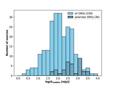
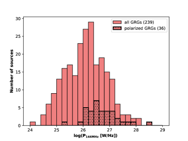
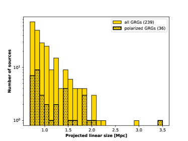
Figure 2: Flux density (top), radio power (center), and projected linear scale (bottom) distributions of the LoTSS DR1 GRG catalog (Dabhade et al., 2020) compared with the 36 GRGs detected in polarization at 144 MHz within this sample.

Figure 3: Detection rate as function of the projected linear size of the GRGs from the distribution shown in the bottom panel of Fig. 2. The widths of the bins are computed to contain the same total number of sources ($\sim$60). Markers are positioned at center of each bin and the error bars show the bin width.

The 37 GRGs are displayed in Fig. 9. Contours show the total intensity. The left-hand panel is the total intensity image at 20$\arcsec$ resolution, the central panel is the LOFAR fractional polarization at 45$\arcsec$ resolution, the right-hand panel is the NVSS fractional polarization at 45$\arcsec$. The color scale and limits are the same per source for both fractional polarization images. In all three images the cyan squares mark the component detected at 20$\arcsec$, cyan points mark the peak of polarized intensity at 20$\arcsec$ (where we derived the RM and fractional polarization values) while magenta points mark the position where we extracted the depolarization factors. The separation between these two points is always within the 45$\arcsec$ resolution element.

3C 236 (GRG 0) was not present in the original GRG catalog by Dabhade et al. (2020). Since it was selected only because its polarization at low frequencies was studied in previous work (e.g., Mack et al., 1997), it is not included in the following paragraphs where we compute the polarization detection rates.

Out of the 36 polarized sources in the GRG catalog, 33 are FR II type sources, 2 are FR I (i.e., GRG 51 and GRG 57), and GRG 136 has a peculiar morphology (see Tab. 6). Only 6 of them have a quasar host, while all the others are radio galaxies (Dabhade et al., 2020). In 75$\%$ of cases the detection is coincident with the hotspots of FR II radio galaxies. This is consistent with the fact that compact emission regions probe smaller Faraday depth volumes and are thus less depolarized. In 19$\%$ of cases, the polarized emission is detected from the more diffuse lobe regions. In these cases, the hotspots may have a lower intrinsic fractional polarization than the lobes. In one case (GRG 117) we detected polarization coincident with the core within our spatial resolution. Since the core of a radio galaxy is not expected to be significantly polarized, this may be a restarted radio galaxy (e.g., Mahatma et al., 2019) with polarized emission arising from the unresolved inner jets. The other detections are from the outer edge of FR I type galaxies and from the extended lobe of the peculiar GRG 136.

The histogram distributions of total radio flux density, total radio power, and projected linear size of the whole sample of 239 GRGs are shown in Fig. 2, together with the distribution of polarized ones. The GRGs detected in polarization have S${}_{\rm 144MHz}\geq$ 56 mJy in total intensity, suggesting a selection effect due to the sensitivity of the survey. Out of the 239 GRGs in the parent sample, 179 sources have S${}_{\rm 144MHz}>$ 50 mJy: above this threshold the detection rate is thus the $20.1\ \%$. With a lower flux density limit of 10 mJy (i.e., 223 GRGs), the detection rate is $16.1\ \%$.

The preliminary LoTSS polarized point-source catalog compiled by Van Eck et al. (2018) obtained a $\ll 1\%$ polarization detection rate for all the sources in the DR1 with total flux densities above 10 mJy (see also O’Sullivan et al., 2018a). Our results cannot be directly compared with this work because of the different resolution and the peculiar nature of GRGs. While the majority of the sources in our sample has a large physical and also angular extent, the detection rate computed by Van Eck et al. (2018) takes into account more compact sources. Furthermore, Van Eck et al. (2018) used preliminary LoTSS images with 4.3$\arcmin$ angular resolution. In-beam depolarization, due to the mixing of different lines-of-sight into the same resolution element, can substantially affect the detection rate. Despite their large physical size, only 29 GRGs out of 239 are larger than 4.3$\arcmin$. All the others are unresolved in the Van Eck et al. (2018) catalog, and thus suffer from the same in-beam depolarization as more compact AGN. To better compare our work with Van Eck et al. (2018) we cross-matched the position of the 195 GRGs with angular size lower than 4.3$\arcmin$ with the point source catalog compiled by Van Eck et al. (2018). The cross-match resulted in 11 sources, which are also detected in polarization in this work with $20\arcsec$ resolution. The polarization detection rate of the unresolved GRGs in the Van Eck et al. (2018) catalog is thus $5.6\ \%$ (11/195). A parent population with large physical size has a higher polarization detection rate than the overall AGN population, even if not resolved. The high detection rate within the GRGs sample suggests the presence of a small amount of depolarization (see also Sec. 2.4). Out of the 29 GRGs larger than $4.3\arcmin$, and thus also resolved in the Van Eck et al. (2018) catalog, four are cataloged as point-sources while only GRG 85 has both lobes detected in polarization. We refer the reader to Mahatma et al. (2020, in prep.) for a more complete statistical study of the polarization properties and detection rate of radio galaxies within the LoTSS DR1.

The central panel of Fig. 2 shows a clear selection effect for GRGs with high total radio power. The median radio power of GRGs detected in polarization is 4.07$\times$10²⁶ W/Hz while it is 1.03$\times$10²⁶ W/Hz for undetected sources (1.8$\times$10²⁶ W/Hz considering only sources with flux density above 50 mJy).

The fraction of GRGs detected in polarization increases with the linear size of the source (see Fig. 3), being $31\%$ for the GRGs with physical sizes larger than 1.5 Mpc. This points to a possible decrease in the amount of Faraday depolarization far from the local environment of the host galaxy. In fact, Faraday depolarization decreases far away from the host galaxy and possible groups or clusters of galaxies (Strom & Jaegers, 1988; Machalski & Jamrozy, 2006). However, this effect is conflated with the fact that the majority of sources with linear sizes larger than 1.5 Mpc have high radio power. Using the Kolmogorov-Smirnov (KS) test to compare the linear sizes we found a marginal difference between the samples of detected and undetected GRGs with S${}_{\rm 144MHz}>$ 50 mJy ($p$-value of 0.08). Although beam depolarization may also have a role, the KS test between the angular sizes of detected and undetected sources with S${}_{\rm 144MHz}>$ 50 mJy suggests that they are drawn from a similar distribution ($p$-value of 0.29).

Dabhade et al. (2020) found 21/239 GRGs to be associated with brightest cluster galaxies (BCGs) by cross-matching their catalog with the Wen et al. (2012) and Hao et al. (2010) clusters catalogs. None of them are detected in polarization apart from GRG 85, whose polarization properties were already studied (O’Sullivan et al., 2019). It has a linear size of 3.4 Mpc and probably resides in a small group of galaxies. The localization of the sources in galaxy group or cluster environments seems to be an exclusion criterion for polarization detection at 144 MHz, and this is likely due to the effect of Faraday depolarization.

Polarization, Faraday rotation, and depolarization information for all sources are reported in Tab. 7 when both the lobes are detected, and in Tab. 8 when only one source component is detected. The histograms of RM and fractional polarization of the detected components (considering both lobes and hotspots of single and double detections) are shown in Fig. 4.

Table 2: Results of the polarized intensity study of detected double-lobed sources.

GRG	R.A.	Dec.	P	$\sigma_{QU}$	$p$	RM	D${}_{1.4\ \rm GHz}^{144\ \rm MHz}$
	(deg)	(deg)	(mJy)	(mJy/beam)	($\%$)	(rad/m2)
0a	151.228	35.026	4.5	0.2	11.7 $\pm$ 0.5	3.23 $\pm$ 0.02	0.7 $\pm$ 0.2
0b	151.918	34.687	26.2	0.3	5.40 $\pm$ 0.06	9.071 $\pm$ 0.006	0.126 $\pm$ 0.007
1a	164.276	53.430	44.0	0.2	5.28 $\pm$ 0.02	12.855 $\pm$ 0.002	0.83 $\pm$ 0.02
1b	164.264	53.448	4.69	0.08	2.57 $\pm$ 0.05	12.20 $\pm$ 0.01	0.167 $\pm$ 0.008
2a	164.257	48.613	14.83	0.09	8.56 $\pm$ 0.05	16.940 $\pm$ 0.003	0.70 $\pm$ 0.02
2b	164.339	48.725	1.23	0.07	0.67 $\pm$ 0.04	19.01 $\pm$ 0.04	0.072 $\pm$ 0.007
19a	167.363	53.255	1.5	0.2	3.2 $\pm$ 0.3	11.18 $\pm$ 0.06	0.5 $\pm$ 0.1
19b	167.422	53.211	1.3	0.2	0.75 $\pm$ 0.09	11.39 $\pm$ 0.07	0.088 $\pm$ 0.007
22a	168.399	46.381	0.87	0.09	1.4 $\pm$ 0.2	4.04 $\pm$ 0.06
22b	168.381	46.364	0.48	0.07	0.9 $\pm$ 0.1	4.57 $\pm$ 0.09
51a	180.311	49.384	0.96	0.09	7.4 $\pm$ 0.7	22.03 $\pm$ 0.05	0.13 $\pm$ 0.04
51b	180.380	49.458	3.1	0.1	10.3 $\pm$ 0.3	22.70 $\pm$ 0.02	0.40 $\pm$ 0.09
64a	184.574	53.441	1.9	0.1	0.32 $\pm$ 0.02	15.30 $\pm$ 0.03	0.062 $\pm$ 0.007
64b	184.569	53.477	1.8	0.1	1.28 $\pm$ 0.07	14.57 $\pm$ 0.03	0.21 $\pm$ 0.07
65a	184.659	50.431	33.6	0.2	3.21 $\pm$ 0.02	27.784 $\pm$ 0.003	0.72 $\pm$ 0.02
65b	184.742	50.445	17.0	0.1	3.00 $\pm$ 0.02	26.682 $\pm$ 0.005	0.43 $\pm$ 0.01
77a	186.468	53.153	0.8	0.1	0.73 $\pm$ 0.09	13.10 $\pm$ 0.08	0.07 $\pm$ 0.02
77b	186.514	53.168	1.25	0.09	3.5 $\pm$ 0.3	11.90 $\pm$ 0.04
85a	188.648	53.376	5.95	0.1	4.41 $\pm$ 0.09	7.51 $\pm$ 0.01	0.64 $\pm$ 0.07
85b	188.853	53.247	1.0	0.1	4.5 $\pm$ 0.4	10.08 $\pm$ 0.06	0.12 $\pm$ 0.01
87a	189.208	46.064	1.6	0.1	3.1 $\pm$ 0.2	21.44 $\pm$ 0.04	0.18 $\pm$ 0.03
87b	189.190	46.083	0.8	0.1	1.4 $\pm$ 0.2	16.92 $\pm$ 0.08	0.08 $\pm$ 0.02
91a	190.090	53.581	11.2	0.1	2.86 $\pm$ 0.03	17.952 $\pm$ 0.006	0.185 $\pm$ 0.006
91b	190.027	53.573	10.35	0.09	3.02 $\pm$ 0.03	19.353 $\pm$ 0.005	0.88 $\pm$ 0.09
103a	195.379	54.130	4.53	0.07	1.28 $\pm$ 0.02	13.676 $\pm$ 0.009	0.097 $\pm$ 0.002
103b	195.441	54.145	13.85	0.09	1.71 $\pm$ 0.01	14.017 $\pm$ 0.004	0.61 $\pm$ 0.03
120a	200.110	49.284	0.61	0.07	4.1 $\pm$ 0.4	10.85 $\pm$ 0.06
120b	200.127	49.277	0.48	0.06	6.9 $\pm$ 0.9	10.90 $\pm$ 0.08
144a	204.835	50.982	0.93	0.09	8.4 $\pm$ 0.8	9.05 $\pm$ 0.06
144b	204.847	50.937	0.57	0.08	4.3 $\pm$ 0.6	8.22 $\pm$ 0.08
145a	205.259	49.278	3.18	0.07	2.33 $\pm$ 0.05	10.52 $\pm$ 0.01	0.32 $\pm$ 0.02
145b	205.266	49.258	5.27	0.07	6.68 $\pm$ 0.09	10.002 $\pm$ 0.008	0.71 $\pm$ 0.06
165a	210.762	51.456	2.91	0.07	7.0 $\pm$ 0.2	19.41 $\pm$ 0.01	1.0 $\pm$ 0.3
165b	210.714	51.458	0.97	0.07	1.01 $\pm$ 0.07	17.62 $\pm$ 0.04	0.4 $\pm$ 0.1
166a	210.770	51.749	1.47	0.07	0.87 $\pm$ 0.04	11.38 $\pm$ 0.03	0.096 $\pm$ 0.007
166b	210.851	51.744	1.48	0.07	0.27 $\pm$ 0.01	12.87 $\pm$ 0.03	0.25 $\pm$ 0.03
168a	211.414	54.197	7.6	0.09	8.9 $\pm$ 0.1	14.998 $\pm$ 0.007	1.0 $\pm$ 0.3
168b	211.428	54.173	0.84	0.07	0.27 $\pm$ 0.02	13.34 $\pm$ 0.05	0.13 $\pm$ 0.03
177a	213.511	48.707	2.14	0.07	0.79 $\pm$ 0.02	19.94 $\pm$ 0.02	0.7 $\pm$ 0.2
177b	213.545	48.694	0.51	0.07	0.14 $\pm$ 0.02	19.18 $\pm$ 0.08	0.31 $\pm$ 0.07
222a	222.690	53.000	4.86	0.09	0.80 $\pm$ 0.02	16.91 $\pm$ 0.01	0.45 $\pm$ 0.07
222b	222.761	53.005	1.35	0.08	0.29 $\pm$ 0.02	15.19 $\pm$ 0.04	0.12 $\pm$ 0.02
233a	226.152	50.501	3.0	0.2	3.5 $\pm$ 0.2	6.16 $\pm$ 0.03	0.044 $\pm$ 0.003
233b	226.225	50.505	2.4	0.2	0.88 $\pm$ 0.06	5.71 $\pm$ 0.04	0.25 $\pm$ 0.04

Table 3: Results of the polarized intensity study for sources with a single polarized detection.

GRG	R.A.	Dec.	P	$\sigma_{QU}$	$p$	RM	D${}_{1.4\ \rm GHz}^{144\ \rm MHz}$
	(deg)	(deg)	(mJy)	(mJy/beam)	($\%$)	(rad/m2)
7	164.634	51.687	0.81	0.07	2.5 $\pm$ 0.2	21.67 $\pm$ 0.05	0.19 $\pm$ 0.06
44	174.908	47.332	0.54	0.06	5.3 $\pm$ 0.6	22.20 $\pm$ 0.07	0.19 $\pm$ 0.05
47	177.991	49.837	0.59	0.07	0.16 $\pm$ 0.02	16.53 $\pm$ 0.07	0.052 $\pm$ 0.007
57	182.675	53.485	4.69	0.07	5.81 $\pm$ 0.09	12.214 $\pm$ 0.009	0.70 $\pm$ 0.09
80	187.512	53.531	0.57	0.06	1.0 $\pm$ 0.1	10.71 $\pm$ 0.07	0.13 $\pm$ 0.04
83	188.252	49.119	1.14	0.08	1.19 $\pm$ 0.08	13.56 $\pm$ 0.04	0.037 $\pm$ 0.004
112	197.578	52.222	0.86	0.09	1.8 $\pm$ 0.2	3.19 $\pm$ 0.06
117	199.144	49.544	1.2	0.07	3.0 $\pm$ 0.2	13.00 $\pm$ 0.03	0.19 $\pm$ 0.02
122	200.906	47.511	0.61	0.079	3.4 $\pm$ 0.4	7.47 $\pm$ 0.07	0.21 $\pm$ 0.05
136	203.374	53.521	1.1	0.1	11.0 $\pm$ 1.0	10.91 $\pm$ 0.07	0.050 $\pm$ 0.009
137	203.561	55.013	0.76	0.08	0.073 $\pm$ 0.008	8.05 $\pm$ 0.06
148	206.071	48.787	0.8	0.1	0.8 $\pm$ 0.1	12.50 $\pm$ 0.07	0.045 $\pm$ 0.004
149	206.178	50.395	1.1	0.08	7.1 $\pm$ 0.5	10.45 $\pm$ 0.04	0.4 $\pm$ 0.2
207	220.024	55.487	0.56	0.06	2.0 $\pm$ 0.2	11.64 $\pm$ 0.07	0.26 $\pm$ 0.07
234	226.541	51.591	0.93	0.09	2.1 $\pm$ 0.2	9.74 $\pm$ 0.06	0.27 $\pm$ 0.06

Figure 4: Distribution of Faraday rotation measure (left), fractional polarization (center), and depolarization factor between 1.4 GHz and 144 MHz (right) of the 59 components (lobes, hotspots, and core) detected in polarization.

3.1 RM difference between lobes

The observed RM is derived from the main peak of the Faraday spectrum at each pixel because all the detected components show a simple Faraday spectrum (i.e., with a single and isolated peak, contrary to the complex Faraday spectrum where multiple peaks are observed, e.g., in Stuardi et al. 2019). In this case, the RM is equal to the Faraday depth, a physical quantity given by:

$$\phi=0.812\int_{\rm{source}}^{\rm{observer}}{n_{e}B_{\parallel}{\rm d}l}\quad\rm{[rad\ m^{-2}]}\leavevmode\nobreak\ ,$$ (1)

where $n_{e}$ is the thermal electron density in cm^-3, $B_{\parallel}$ is the magnetic field component parallel to the line of sight in $\mu$G, and ${\rm d}l$ is the infinitesimal path length in parsecs.

The values of RM obtained are between 3 and 28 rad m^-2 with a median value of 12.8 rad m^-2 (see left panel of Fig. 4). The fact that they are all positive points out that in the sampled 424 deg² sky region the magnetic field of our Galaxy is pointing toward us and it is the dominant source of the mean Faraday rotation. This implies a smooth Galactic magnetic field on scales of $\sim$10 deg (i.e., the median distance between the sources).

Among the 36 detected sources, 21 GRGs have both lobes detected in polarization (at least one above the 8$\sigma$ significance level). For these sources, plus GRG 0, we computed the RM difference between the two lobes ($\Delta$RM). This quantity indicates a difference in the intervening magneto-ionic medium on large scales (of the order of 1 Mpc at the redshifts of the sources). $\Delta$RM can be caused by variations in the Galactic RM (GRM), in addition to a different line-of-sight path length between the two lobes in the local environment and/or differences in the IGM on large scales.

Figure 5: Squared RM difference versus angular (left) and physical (right) separation between the detected lobes. A number corresponds to each GRG and the numbers are listed in Tab. 7. The blue dashed line is the power-law fit to the data with 1$\sigma$ uncertainty (see Sec. 3.1). Orange bars shows binned averages between 1.5$\arcmin$ and 20$\arcmin$ obtained by Vernstrom et al. (2019) for physical pairs observed at 1.4 GHz and the dashed orange line shows the derived structure function. Blue bars show the binned averages of the sources in this work with angular separation lower than $10\arcmin$: each bin contains 10 sources, the uncertainty is computed as the standard deviation on the mean. Shadowed areas show the uncertainties.

The reconstruction of the GRM by Oppermann et al. (2015) has a resolution of 1^∘ (i.e., the typical spacing of extra-galactic sources in the Taylor et al. 2009 catalog) so that most of our double-lobed GRGs lie in the same resolution element of the reconstruction. All the measured RMs are within the 3$\sigma$ error of the estimated GRM, with the exception of GRG 144, for which the difference is within the 4$\sigma$ error. The average of the GRM values at the position of the detected components (i.e., on scales of of $\sim$10 deg) is 13$\pm$1 rad m^-2: consistent with the one found from our measurements. Due its low angular resolution this map cannot be used to probe RM variations on scales smaller than 1^∘ for selected sources. However, RM structure function studies (i.e., $<\Delta{\rm RM}^{2}>$ versus angular separation) have probed the RM variance on scales below 1^∘, but with large uncertainties (Stil et al., 2011; Vernstrom et al., 2019). The GRM variance was found to have a strong dependence on angular separation, in particular at low Galactic latitude. The 22 double GRGs have angular separations ($\delta\theta$) ranging between $\sim$1.8$\arcmin$ and $\sim$40$\arcmin$ and they all have Galactic latitude above 50^∘, with GRG 0 being the largest in size and closest to the Galactic plane. The study of $\Delta$RM² as a function of angular separation in our sample can be used to understand if the RM difference is dominated by the turbulence in the Galactic interstellar medium.

$\Delta$RM² is plotted against the angular separation of the lobes in the left panel of Fig. 5. Despite the large scatter at low angular separation, a general increasing trend of $\Delta$RM² with $\delta\theta$ is observed. We computed the average $\Delta$RM² for the sources with $\delta\theta<10\arcmin$ (thus excluding GRG 85 and GRG 0) divided in two bins with 10 sources each (uncertainties are computed as the standard deviation on the mean). The binned averages are over-plotted in Fig. 5. We fitted a power law of the form:

$$\Delta{\rm RM}(\delta\theta)^{2}=A\delta\theta^{B}\ ,$$ (2)

and we obtained: $A=0.56\pm 0.06$ rad² m^-4 and $B=1.1\pm 0.1$ with $\chi^{2}=515$ (the blue line in Fig. 5). The fit suggests an increasing influence of the Milky Way foreground with angular size. However, it is dominated by a few GRG with the largest angular sizes and more sources at large $\delta\theta$ would be required to confirm this behavior. Conversely, the binned average for sources at low angular separation shows a large scatter and points to a flattening of the power-law slope for $\delta\theta<2\arcmin$. This could be related to an increasing influence of the extra-galactic contribution over the Galactic one at small angular scales.

We can compare our result with the structure function studies of Stil et al. (2011) and Vernstrom et al. (2019). While Stil et al. (2011) considered together all kinds of source pairs (physical and non-physical), Vernstrom et al. (2019) separated physical and non-physical pairs. The latter is thus best suited for a direct comparison with our work where all pairs are physical. Vernstrom et al. (2019) made use of the Taylor et al. (2009) catalog of polarized sources observed at 1.4 GHz. For a sample of 317 physical pairs with angular separations between $1.5\arcmin$ and $20\arcmin$ they obtained $A=11\pm 15$ rad² m^-4 and $B=0.8\pm 0.2$. The fit is shown as a comparison in the left hand panel of Fig. 5. The slopes are consistent within the 2$\sigma$ uncertainty. The slightly steeper power-law compared to the one obtained by Vernstrom et al. (2019) can be attributed to the presence of GRG 0 in our sample. In both cases the trend is dominated by pairs of sources at $\delta\theta>10\arcmin$, indicating an increasing contribution from the GRM.

Due to their large size, GRGs are expected to lie at large angles to the line of sight and to extend well beyond the group/cluster environment so that the differential Faraday rotation effect originating in the local environment should be minimal (Laing, 1988; Garrington et al., 1988). Furthermore, none of our sources show a prominent one-sided large-scale jet that would indicate motion toward the line of sight, not even the six sources with a quasar host (i.e., GRG 1, GRG 47, GRG 91, GRG 120, GRG 137, GRG 222 ). Thus, $\Delta$RM is not expected to strongly correlate with the source physical size. However, to investigate the local contribution, we plotted the RM difference squared against the physical separation between the two lobes (Fig. 5, right panel). Notable is the similarity between the right-hand and left-hand panel of Fig. 5. If the main contribution was due to the local environment, we would typically expect a larger RM difference between the lobes at smaller physical separations. Conversely, the similarity between the panels of Fig. 5 suggests that this trend is dominated by the angular separation trend, which is driven by Galactic structures. This points out that the local environment is sub-dominant in determining $\Delta$RM.

Asymmetries in the foreground large-scale structures could also contribute to the RM difference between the two lobes. We expect much more large-scale asymmetries close to galaxy clusters (Böhringer et al., 2016). We note that, according to the environment analysis of Dabhade et al. (2020), none of the GRGs detected in polarization are associated with the BCG of a dense cluster of galaxies. However, foreground galaxy clusters are Faraday screens for all the sources that are in the background. Therefore, we cross-matched the position of the 22 GRGs with the cluster catalog of Wen & Han (2015) in order to find the foreground galaxy cluster at the smallest projected distance from each GRG. This catalog is based on photometric redshifts from the SDSS III and lists clusters in the redshift range 0.05 $<z<$ 0.8. In the redshift range 0.05 $<z<$ 0.42 it is 95$\%$ complete for clusters with mass M${}_{200}>10^{14}$ M_⊙. Taking into account the uncertainty on the photometric redshift estimates, $\Delta z=0.04(1+z)$, we considered a cluster as being in the foreground of a particular GRG for all clusters with $z-\Delta z$ lower than the redshift of the GRG plus its uncertainty.

We computed the angular separation between each GRG lobe and the closest foreground galaxy cluster ($\delta\theta^{\rm min}_{\rm cluster}$ and $\delta\theta^{\rm max}_{\rm cluster}$, for the closest and farthest lobe, respectively). $\Delta$RM² is plotted against $\delta\theta^{\rm min}_{\rm cluster}$ divided by angle subtended by $R_{500}$ of the cluster ($\theta_{R_{500}}$, in arcminutes) in the top panel of Fig. 6. Most of the GRGs lie at projected distances larger than $R_{500}$ and the trend does not show a clear dependence of $\Delta$RM on the distance from the closest foreground cluster. Asymmetries in the foreground large-scale structures are thus probably sub-dominant compared to the ones caused by the GRM. However, this will be further discussed in Sec. 4.

3.2 Faraday depolarization

RM fluctuations within group and cluster environments can be caused by turbulent magnetic field fluctuations over a range of scales. While large scale fluctuation are mostly responsible for the RM difference between the lobes, fluctuation on the smallest scale may be at the origin of Faraday depolarization. The mixing of different polarization vector orientations within the observing beam and along the line of sight reduces the fractional polarization. The RM dispersion for a simple single-scale model of randomly orientated magnetic field is

$$\sigma_{\rm RM}^{2}=0.812^{2}\Lambda_{c}\int_{\rm{source}}^{\rm{observer}}{(n_{e}B_{\parallel})^{2}{\rm d}l}\quad\rm{[rad^{2}\ m^{-4}]}\leavevmode\nobreak\ ,$$ (3)

where $\Lambda_{c}$ is the correlation length of the magnetic field in parsecs (e.g., Felten, 1996; Murgia et al., 2004). The RM dispersion is responsible for the Faraday depolarization which in the case of an external screen (Burn, 1966) is expressed as:

$$p(\lambda)=p(\lambda=0)e^{-2\sigma_{\rm RM}^{2}\lambda^{4}}\leavevmode\nobreak\ .$$ (4)

In the GRGs sample, the fractional polarization at 20$\arcsec$ resolution ranges between 0.07 and $11.7\ \%$ with a median value of $2.6\ \%$ (see central panel of Fig. 4). LOFAR has a unique capability to reliably detect very low fractional polarization values (i.e., $<0.5\ \%$) when RM is outside the range $-3<\phi<1$ rad m^-2 because of the high resolution in Faraday space that allows a clear separation from the leakage contribution.

Four components detected at 20$\arcsec$ are under the detection threshold at 45$\arcsec$. This is due to the lower sensitivity at 45$\arcsec$ resolution. Only in one case (GRG 112) is the non-detection likely caused by beam depolarization on scales between 20$\arcsec$ and 45$\arcsec$ (i.e., 140 and 315 kpc at the source redshift). Instead, five sources are not detected in the NVSS due to the lower sensitivity of this survey. Hence, there are 28 sources with depolarization measurements. The distribution of depolarization factors computed at 45$\arcsec$ is shown in the right panel of Fig. 4. All the sources have D${}_{1.4\ \rm GHz}^{144\ \rm MHz}$¿0.03 and the median value is 0.2.

Our measurements enable us to probe magnetic field fluctuations on scales below the 45$\arcsec$ restoring beam, which for the redshift range of our sample corresponds to physical scales of 80-480 kpc. Faraday depolarization can occur internally to the source or can be due to the small-scale fluctuation of the magnetic field in the medium external to the source.

With LoTSS data, we are not able to observe internal depolarization, that would appear as a thick Faraday component through RM-synthesis. This is because the largest observable Faraday scale is smaller than the resolution in Faraday space (see Sec. 2.2). Broad-band polarization studies at higher frequencies and/or detailed modeling of internal Faraday screens would be needed to distinguish between these two scenarios.

In the case of external depolarization, Eq. 4 implies that the effect of a $\sigma_{\rm RM}\leq 1$ rad m^-2 is only observable at very large wavelengths. For this reason, by comparing measurements at 1.4 GHz and at 144 MHz it is possible to study the depolarization caused by low $\sigma_{\rm RM}$. On the other hand, $\sigma_{\rm RM}\geq 1$ rad m^-2 can completely depolarize the emission and make it undetectable by LOFAR. Within galaxy clusters, where $B\sim 0.1-10\ \mu$G, $n_{e}\sim 10^{-3}$ cm^-3 and the magnetic field is tangled on a range of scales, the RM dispersion is clearly above this level (e.g., Murgia et al., 2004; Bonafede et al., 2010).

The distribution of distances from the closest foreground cluster is compared for detected and undetected GRGs in polarization in the top panel of Fig. 7 while the detection rate is computed as function of the distance from the foreground cluster in the bottom panel (for GRGs with S${}_{\rm 144MHz}>$ 50 mJy). We find that $8\ \%$ of the GRGs observed within 2$R_{500}$ of the closest foreground cluster are detected in polarization, while the detection rate increases to $27\ \%$ outside 2$R_{500}$. The Kolmogorov-Smirnov test indicates a significant difference between the samples of detected and undetected GRGs with S${}_{\rm 144MHz}>$ 50 mJy ($p$-value of 2$\times 10^{-3}$). Together with the non detection of the GRGs at the center of clusters (Sec. 3), this shows that in general, to be detected by the LoTSS, sources need to avoid locations both within and in the background of galaxy clusters where the RM dispersion is too high.

Only four GRGs are detected within $R_{500}$: GRG 2, GRG 91, GRG 120, and GRG 136. Among them, GRG 2 ($z=0.27627\pm 0.00005$) and GRG 136 ($z=0.354\pm 0.034$) have similar redshifts with respect to the clusters (at redshifts $0.27\pm 0.05$ and $0.37\pm 0.05$, respectively). They have been considered in the background due to the uncertainties on the photometric redshift estimates, but it is also possible that these GRGs are cluster members or instead lie in the foreground of the clusters. GRG 91 and GRG 120 are associated with compact foreground clusters with $R_{500}$ equal to 570 kpc and 650 kpc respectively.

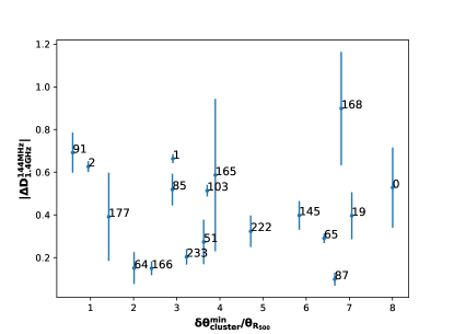
Figure 6: Squared RM difference (top panel) and depolarization factor difference between the two lobes (bottom panel) versus the minimum distance from the closest foreground galaxy cluster scaled by $R_{500}$ of the cluster.

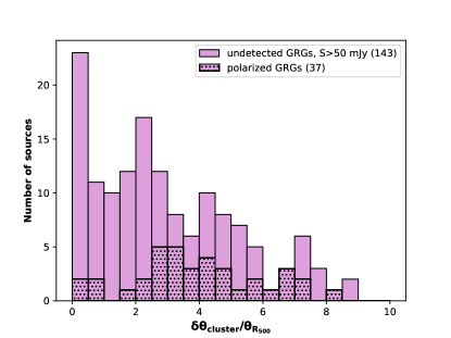
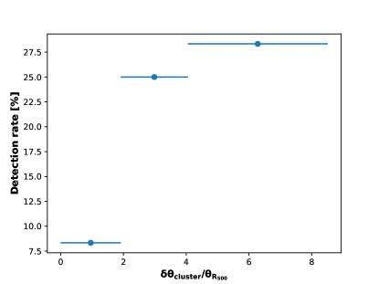
Figure 7: Distribution of minimum distance from the closest foreground cluster for detected and undetected sources in polarization (top panel), and detection rate as function of the minimum distance from foreground clusters (bottom panel). The widths of the bins are computed to contain the same total number of sources (i.e., 60). Markers are positioned at center of each bin and the error bars show the width of the bins.

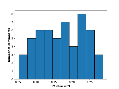
Figure 8: Distribution of RM dispersion values obtained using an external Faraday screen model.

Using D${}_{1.4\ \rm GHz}^{144\ \rm MHz}$ in Eq. 4 we can compute $\sigma_{\rm RM}$. The distribution of $\sigma_{\rm RM}$ is shown in Fig. 8. The maximum value is 0.29 rad m^-2. Given the small amount of depolarization it is important to consider that the residual error in the ionospheric RM correction within the 8 hours of the observation could account for $\sim 0.1-0.3$ rad m^-2 (Van Eck et al., 2018). In principle, this could explain most or all the depolarization observed but we can test this because the residual ionospheric correction error is subtracted out in the difference in depolarization between the two hotspots of the same radio galaxy. —$\Delta$ D${}_{1.4\ \rm GHz}^{144\ \rm MHz}$— represents a lower limit to the depolarization that leads to $\sigma_{\rm RM}$ values between 0.05 and 0.25 rad m^-2. These estimates are further discussed in Sec. 4.

We have tested the possibility that the closest foreground cluster was the main origin of the measured depolarization by plotting —$\Delta$ D${}_{1.4\ \rm GHz}^{144\ \rm MHz}$— versus the distance from the cluster in the bottom panel of Fig. 6. However, we do not find a correlation between these quantities.

D${}_{1.4\ \rm GHz}^{144\ \rm MHz}$is also not correlated with the distance from the host galaxy, probably because all the sources are very extended and already well beyond the host galaxy’s halo (Strom & Jaegers, 1988). The Laing-Garrington effect (i.e., the differential Faraday depolarization that causes the counter-lobe to be more depolarized than the lobe closer to us Laing 1988; Garrington et al. 1988) is indeed not expected to be a strong effect in this case. We note that none of the GRGs show a prominent jet in the total intensity images (see Fig. 9), which is in line with the expectation that these sources are observed at large angles to the line of sight.

4 Discussion

Since both RM and depolarization are integrated effects along the line of sight (Eq. 1 and 3), in order to disentangle the contribution of the different Faraday rotation and depolarization screens one should have detailed information on the environment surrounding each radio galaxy, the foreground, and the geometry and physical properties of the lobes. This requires a detailed study of each single source. We instead investigated several possible origins of the RM difference and Faraday depolarization considering the correlation of $\Delta$RM and D${}_{1.4\ \rm GHz}^{144\ \rm MHz}$ with different physical quantities.

Several statistical analyses on the RMs of extra-galactic sources have been performed. Structure function studies verified the dependence of $\Delta$RM on the angular separation originated by the Galactic magnetic field (e.g., Simonetti et al., 1984; Sun & Han, 2004; Stil et al., 2011). The presence of a growing contribution to the RM with redshift was investigated by Pshirkov et al. (2015). The RM variance of background sources was modeled to separate an extra-galactic contribution of 6-7 rad m^-2 from the Galactic one (e.g., Schnitzeler, 2010; Oppermann et al., 2015). Bringing together these works, Vernstrom et al. (2019) studied the average $\Delta$RM² as function of angular separation, redshift, spectral index, and fractional polarization using two large samples of physical and non-physical pairs in order to isolate the extra-galactic contribution. A difference of $\sim 10$ rad m^-2 in the average $\Delta$RM² between the two samples was attributed to the IGM to derive an upper limit on the extra-galactic magnetic field of 40 nG. A contribution from the local magnetic field, producing a larger variance for non-physical pairs, cannot be excluded. All these studies were performed at 1.4 GHz, thanks to the presence of the RM catalog produced with the NVSS (Condon et al., 1998; Taylor et al., 2009). With the advent of LOFAR, these kind of studies are also possible at low frequencies. With respect to the NVSS, the LoTSS allows a better resolution, sensitivity, and precision in the RMs determination.

In this work, the RM difference between the lobes was found to be marginally correlated with the angular distances of the lobes (Fig. 5). Although the correlation is not strong (with a Spearman correlation coefficient of 0.35), we found the relation between $\Delta$RM² and $\delta\theta$ to be consistent with the Galactic structure function found by Vernstrom et al. (2019) for physical pairs. This strongly suggests a Galactic origin of the $\Delta$RM between the lobes. The accuracy in the determination of the amplitude parameter is 250 times higher than the one obtained using NVSS measurements. The same trend observed with the angular separation dominates also the correlation between $\Delta$RM and physical distance. This suggests that the local gas densities and magnetic fields, which should have a stronger effect on the RM variation for normal size galaxies, are not dominant in this sample. This would also explain the fact that, although consistent within the errors, the amplitude of the power-law at 144 MHz is one order of magnitude lower than the one at 1.4 GHz (see Fig. 5). While in Vernstrom et al. (2019) the physical size of the sources is no taken into account, our GRG sample constitutes a population where the local contribution to $\Delta$RM is negligible. A selection of a source population with low local RM variance is an important requirement for future RM grid experiments (Rudnick, 2019).

Recently, O’Sullivan et al. (2020) applied the same method of Vernstrom et al. (2019) to the RMs derived at 144 MHz from the LoTSS. This study resulted in an extra-galactic contribution of 0.4$\pm$0.3 rad m^-2 which yielded to an upper limit on the co-moving magnetic field of 2.5 nG. Since the magnetic field in the IGM is not expected to vary with frequency, the discrepancy between the results obtained at 1.4 GHz and 144 MHz was attributed to the Faraday depolarization effect. Since a high local RM variance can depolarize sources below the detection level at low frequencies, observations at 144 MHz selects sources with low RM variance which unveils the effect of weaker magnetic fields and lower thermal gas densities.

To measure and investigate the origin of the depolarization is thus complementary to the aforementioned studies. In this context, the depolarization is caused by RM variance on scales of the synthesized beam which consequently affect the measurement of the RM variance on the scale of the angular separation between the sources (or the sources’ lobes). The dependence of the RM variance and depolarization on the physical size of classical double radio sources was investigated by Strom & Jaegers (1988) and Johnson et al. (1995) to study the local magnetic field. Machalski & Jamrozy (2006) extended this work by comparing normal size and giant radio galaxies, finding that the depolarization factor strongly correlates with the size of the sources. Within the GRG sample collected by Machalski & Jamrozy (2006) the median depolarization factor between 4.9 GHz and 1.4 GHz is 1.04$\pm$0.05, with the majority of sources showing undetectable levels of depolarization. The RMs, obtained with a fit between the two frequencies and thus subject to the $n\pi$ ambiguity, are also consistent with 0 within the large uncertainties. The wavelength at which substantial depolarization occurs increases with the size of the sources. The depolarization caused by a $\sigma_{\rm RM}\sim 0.3$ rad m^-2 would be undetected at GHz frequencies. Low-frequency observation are thus necessary to measure the small amount of depolarization experienced by the lobes of GRGs in order to constrain the magneto-ionic properties of their environment.

While RM differences between the lobes probe magnetic field fluctuations on large scales (i.e., $\sim$1 Mpc) the depolarization is sensitive to angular scales below the 45$\arcsec$ resolution. This implies scales of 80-480 kpc in the redshift range of the sources. In the most common model of external Faraday dispersion, the depolarization roughly scales as 1/$\sqrt{N}$ where $N$ is the number of Faraday cells within the beam (Sokoloff et al., 1998). A model of random magnetic field fluctuations in $N$=25 cells is able to explain the median D${}_{1.4\ \rm GHz}^{144\ \rm MHz}$=0.2 and it implies a magnetic field reversal scale of 3-25 kpc.

The depolarization observed is thus most likely occurring in a very local environment. This is also supported by Fig. 3 which shows an increasing detection rate with larger distances from the host galaxy and thus from the local enhancement of gas density. A simple model of constant thermal electron density of $\sim 10^{-5}$ cm^-3 and magnetic field of $\sim 0.1\ \mu$G tangled on scales of 3-25 kpc could explain the values of $\sigma_{\rm RM}$ observed using Eq. 3 with an integration length ¡ 100 kpc. Sub-$\mu$G magnetic fields and thermal electron densities of a few times $10^{-5}$ cm^-3 are consistent with the findings from detailed studies on single giant radio galaxies (e.g., Willis et al., 1978b; Laing et al., 2006). From the study of five well known GRGs, Mack et al. (1998) also concluded that the density estimates in the environments of these sources are one order of magnitude lower than within clusters of galaxies. This is the typical environment that polarization observations with LOFAR allow us to study, since larger $\sigma_{\rm RM}$ would completely depolarize the emission. This automatically excludes all the source lying within dense cluster environment, as confirmed by the fact the all 21 GRGs known to reside in clusters are undetected in polarization. Sources residing in such under-dense environment are thus the dominant population of physical pairs also in the work by O’Sullivan et al. (2020).

We note that the $\sigma_{\rm RM}$ values shown in Fig. 8 were derived assuming external depolarization (Eq. 4). With measurements at only 144 MHz and 1.4 GHz, we can not exclude other depolarization models (e.g., Sokoloff et al., 1998; Tribble, 1991; O’Sullivan et al., 2018b). A detailed depolarization analysis with a larger wavelength-square coverage would be needed. For example, in the case in which the polarized emission at 144 MHz originates from an unresolved region within the 45$\arcsec$ beam across which the RM gradient is effectively zero and the rest of the polarized structure is completely depolarized by RM fluctuations, our $\sigma_{\rm RM}$ estimates are not applicable. This would imply that the true $\sigma_{\rm RM}$ of the local environment could be much higher but that our measurements at 144 MHz cannot detect this emission.

4.1 The influence of foreground Galaxy Clusters

Having investigated the Galactic and local Faraday effects on $\Delta$RM and D${}_{1.4\ \rm GHz}^{144\ \rm MHz}$ and their implication for present and future polarization studies with LOFAR, we shift our attention to the possible presence of Faraday screens in the foreground of our targets. Several statistical studies of the Faraday rotation of background sources have demonstrated the presence of magnetic field in clusters of galaxies (e.g., Lawler & Dennison, 1982; Clarke et al., 2001; Böhringer et al., 2016). The scatter in the RMs was found to be enhanced by the cluster magnetic field up to 800 kpc from the cluster center (Johnston-Hollitt & Ekers, 2004). The majority of the double detected sources in our study lies outside R₅₀₀ of foreground clusters (see Fig. 6). Therefore, it is not surprising that the correlation between $\Delta$RM² and the distance from the closest foreground cluster is rather weak (Spearman correlation coefficient of 0.11). In any case, because of LOFAR’s high sensitivity to small RMs, LOFAR allows us to explore regions far outside galaxy clusters which are traced by the lobes of GRGs.

We can use a $\beta$-model (Cavaliere & Fusco-Femiano, 1976) to describe the gas density profile in clusters: $n(r)=n_{0}(1+r^{2}/r_{c}^{2})^{-3\beta/2}$, where we assume the central gas density, $n_{0}\sim 10^{-3}$ cm^-3, the core radius, $r_{c}\sim 200$ kpc, and $\beta$=0.7. We assume that the magnetic field strength scales with the gas density: $B(r)=B_{0}(n(r)/n_{0})^{0.7}$ and that $B_{0}\sim 3\ \mu$G (Dolag et al., 2001; Bonafede et al., 2010; Govoni et al., 2017). The choice of these parameters is somewhat arbitrary but they can reasonably describe galaxy cluster environments. Less massive clusters have a lower electron column density along the line of sight for a given radius scaled by $R_{500}$ and in our sample $R_{500}$ ranges between 0.56 and 1.01 Mpc. Considering a median $R_{500}\sim 800$ kpc, outside the projected distance of 4 times $R_{500}$ the thermal electron density is ¡ $3\times 10^{-6}$ cm^-3 and the magnetic field strength ¡ 0.05 $\mu$G. Assuming a large magnetic field fluctuation scale of 500 kpc, the mean RM from Eq. 1 is $<0.06$ rad m^-2 (where we used $B_{\parallel}=B/\sqrt{3}$). For GRGs with $\delta\theta^{\rm min}_{\rm cluster}>4\theta_{R_{500}}$ the foreground clusters cannot be the dominant origin of the RM difference since their signature would be too weak even for LOFAR RM accuracy. Therefore, the effect of foreground clusters and large-scale IGMF asymmetries to the RM difference is disfavored but it is still non-negligible for some of the GRGs in our sample.

Three double-detected GRGs lie within R₅₀₀ of the closest foreground cluster, namely GRG 2, GRG 91, and GRG 120. We computed for each of them $\delta\theta^{\rm min}_{\rm cluster}$ and $\delta\theta^{\rm max}_{\rm cluster}$, i.e., the distances of the two lobes from the cluster. GRG 91 is associated with a compact foreground cluster with $R_{500}$ of 570 kpc . While for GRG 2 the two lobes are, respectively, at $\sim$2 and $\sim$0.95 R₅₀₀, the distance of both lobes of GRG 120 from the foreground cluster is $\sim$0.96 R₅₀₀. Using the simplified galaxy cluster model previously assumed we would expect a $\Delta$RM² of $\sim$20 rad m^-2 for GRG 2 and $\sim$0.1 rad m^-2 for GRG 120. Although this model overestimates the observed values, it is able to explain more the two order of magnitude difference between the two sources. This suggests that both the source distance and the difference of distances of the two lobes from foreground clusters can in principle play a role in determining $\Delta$RM. For other sources, i.e., GRG 0 and GRG 87, which lies more than 4R₅₀₀ away from the closest foreground cluster, the enhanced RM difference could also be influenced by the presence of large-scale structure filaments, as proposed for GRG 85 (O’Sullivan et al., 2019). A detailed study of the local environment and of the foreground of the GRGs is required in this cases. Such a study may be addressed in future work. A complementary approach that was used by Mahatma et al. (2020, in prep.) is to invoke a universal pressure profile to predict the distributions of RM toward the population of radio galaxies with local and large-scale contributions

The fractional polarization, and thus depolarization factor, is also known to scale with the distance from the cluster center. Bonafede et al. (2011) performed a study of the polarization fraction of sources in the background of galaxy clusters and found that the median fractional polarization at 1.4 GHz decreases toward the cluster center. The trend is observed up to $\sim 5$ core radii (that, in the framework of the simple cluster model described above, corresponds to 1.25R₅₀₀) while far outside the median fractional polarization reaches a constant value of $\sim 5\ \%$. Fig. 6 (bottom panel) and Fig. 7 show that, while the depolarization does not correlate with the distance from foreground clusters, the presence of the latter disfavors the detection of the sources in polarization. This is consistent with the value of D${}_{1.4\ \rm GHz}^{144\ \rm MHz}$ depending mostly on the magneto-ionic properties of the local environment of each GRG. Within R₅₀₀, the higher RM variance due to the turbulence in the foreground ICM influences the fractional polarization at GHz frequencies and depolarizes the radio emission at 144 MHz below the LoTSS detection limit. It is plausible that only under particular condition some background sources can be detected, for example, when the foreground cluster is poor and/or the polarized emission originates in a very compact region of the source. Thus, the detection rate at 144 MHz is strongly reduced up to 2-2.5 R₅₀₀. This highlights the presence of magnetic field at larger distances from galaxy clusters than was shown by previous studies at higher frequencies (Clarke, 2004). This has also the important consequence that future RM grid studies using the LoTSS will mainly sample lines of sight in the extreme peripheries of galaxy clusters, through filaments and voids.

5 Conclusions

In this work we used data from the LOFAR Two-Metre Sky Survey to perform a polarization analysis of a sample of giant radio galaxies selected by Dabhade et al. (2020). Our aims were to (i) study the typical magnetic field in the environment of this class of sources which is unveiled by their polarization properties at low-frequencies (ii) understand how GRGs can be used in a RM grid to derive important information on foreground magnetic fields. We measured the linear polarization, Faraday rotation measure, and depolarization between 1.4 GHz and 144 MHz of the 37 sources detected in polarization. Compared to previous studies at GHz frequencies, this study allowed us to measure the small amount of Faraday rotation and depolarization experienced by these sources. The high precision in the RM determination ($\sim 0.05$ rad m^-2) enables the detection of very small difference between the lobes of the GRGs ($\Delta$RM) that we studied against the angular and physical separation and the distance from foreground galaxy clusters. Since the Faraday depolarization has a strong impact on the detection rate at 144 MHz, the latter was also used as a tool to investigate the presence of depolarizing screens. Our results are summarized as follows:

1. Among the 179 giant radio galaxies observed at $20\arcsec$ resolution with flux density above 50 mJy, the polarization detection rate is $20\ \%$ above an 8$\sigma_{QU}$ detection threshold. A comparison with the polarized point-source catalog by Van Eck et al. (2018) indicates that sources with large angular size have a much greater chance of being detected. Our study suggests that this class of source preferentially resides in very rarefied environments experiencing low levels of depolarization. GRG represent thus a good sample for targeted polarization studies of the magneto-ionized foreground medium.

2. The RM variation on scales below 40$\arcmin$ was investigated using the RM difference between the lobes of the same galaxy. Our study supports the idea that the main contribution to $\Delta$RM on scales between 2$\arcmin$ and 40$\arcmin$ comes from the Milky Way foreground as obtained by Vernstrom et al. (2019). With respect to previous studies performed at GHz frequencies, our investigation provided two order of magnitude higher precision in the determination of $\Delta$RM. A larger sample of sources would be needed to confirm this trend. Local and foreground galaxy cluster contributions to $\Delta$RM are subdominant but non-negligible for some of the sources.

3. Using NVSS archival data, we studied the depolarization between 1.4 GHz and 144 MHz. We detected Faraday depolarization caused by a Faraday dispersion of up to $\sim$0.3 rad m^-2. Such small amounts of depolarization cannot be detected at higher frequencies. It may occur in the local environment of the lobe/hotspot, due to small-scale (few tens kpc) magnetic field fluctuations. A factor of 10 better ionospheric RM correction would be needed to constrain the true astrophysical depolarization of each source.

4. From our analysis, we observed that the environment of the detected giant radio galaxies is extremely rarefied, with thermal electron densities $<10^{-5}$ cm^-3 and magnetic fields below $\sim 0.1\ \mu$G. This is likely the typical environment of the majority of sources that LOFAR can detect in polarization. Studies of the extra-galactic magnetic field performed with LoTSS (e.g., O’Sullivan et al., 2019) need to take into account a lower local contribution than studies performed at higher frequencies.

5. Furthermore, at LOFAR frequencies the chance of detecting a giant radio galaxy for background RM studies of galaxy clusters is 3 times larger outside 2$R_{500}$ than within it. This indicates that the magnetic field in the outskirts of galaxy clusters has an impact on the polarization of background sources at larger distances than previously observed (Bonafede et al., 2011).

This work shows the polarization and RM properties of the largest class of sources detected by LOFAR in polarization, and highlights the potential of their use to study the magneto-ionic properties of large-scale structures. A denser RM grid is needed to constrain the extra-galactic contribution to the RM variance. Future studies, on the basis of thousands of RMs with known redshifts detected by the LoTSS, will enable us to probe the weak signature of the intergalactic magnetic field both in the peripheries of, and far outside, galaxy cluster environments.

Appendix A Images

The images of all the GRGs detected in polarization are shown in Fig. 9. We show the total intensity images at 20$\arcsec$ resolution and the fractional polarization images at $45\arcsec$ compared with the NVSS fractional polarization images at 1.4 GHz. In some cases the detected regions appear as a few scattered pixels that are not beam-shaped. This is a consequence of having peak polarized intensities very close to the detection threshold cutoff.

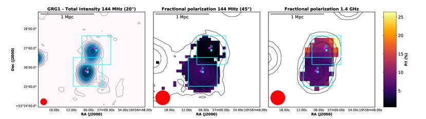
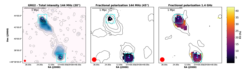
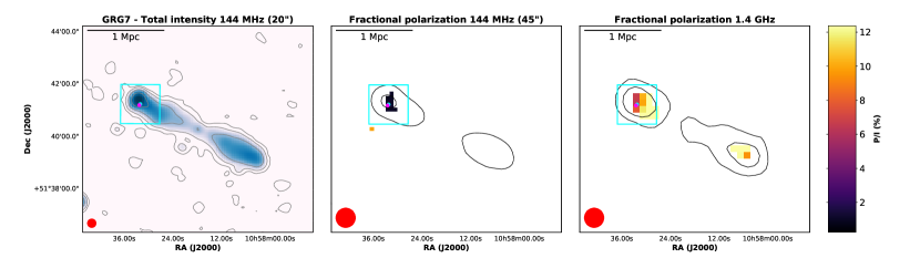
Figure 9: Images of the GRGs detected in polarization. Left: LoTSS total intensity image at 20$\arcsec$ resolution with contours overlaid. Contours start at 3$\sigma$ noise level and are spaced by a factor of four (with $\sigma$ ranging between 0.09 and 0.9 mJy/beam). Center: LoTSS fractional polarization at 45$\arcsec$ resolution with total intensity contours overlaid. Contours start at 3$\sigma$ noise level and are spaced by a factor of four (with $\sigma$ ranging between 0.1 and 8 mJy/beam). Only pixels above the $8\sigma_{QU}$ detection threshold in polarization are shown (except for GRG 78, for which the threshold is at 7 times $\sigma_{QU}$, and GRG 80 and GRG 87, for which it is 6$\sigma_{QU}$). Right: NVSS fractional polarization with total intensity contours overlaid. Contours start at 3$\sigma$ noise level and are spaced by a factor of four (with $\sigma$ ranging between 0.2 and 0.7 mJy/beam). Only pixels with signal-to-noise higher than three in polarization are shown. The color scale and limits are the same in both $P$/$I$ images for each source. The cyan squares mark the component detected at 20$\arcsec$, cyan points mark the peak of polarized intensity at 20$\arcsec$ (RM and fractional polarization values at this position are listed in Tab. 7 and Tab. 8) while magenta points mark the position where we computed the depolarization factors. Letters mark the two components listed in Tab. 7 for double-lobed detected sources.

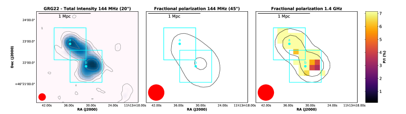
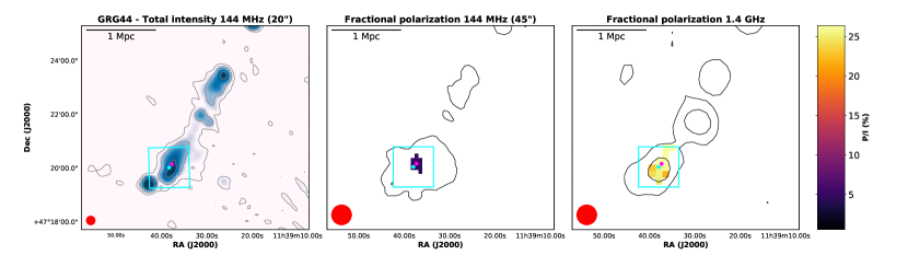
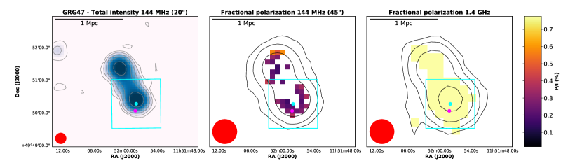
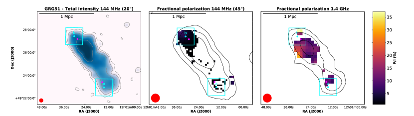
Figure A9 (continued):

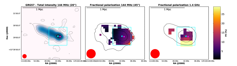
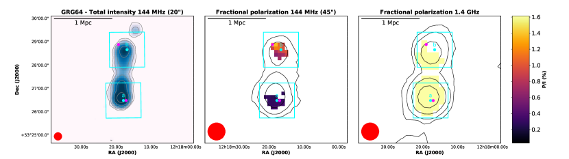
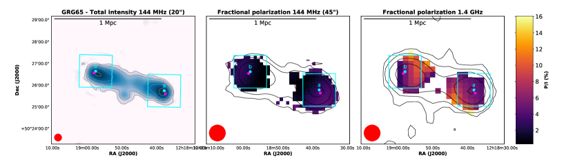
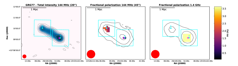
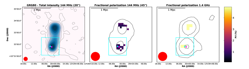
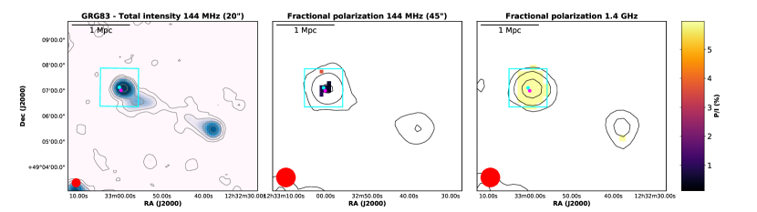
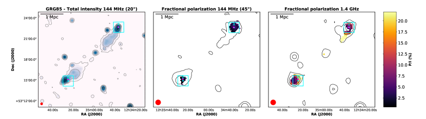
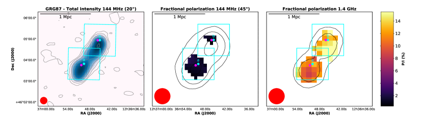
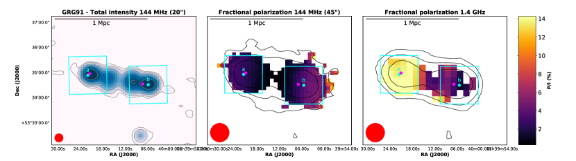
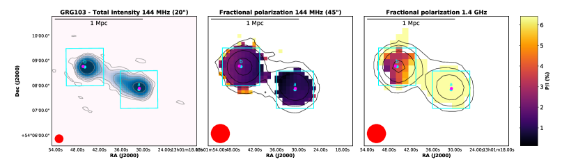
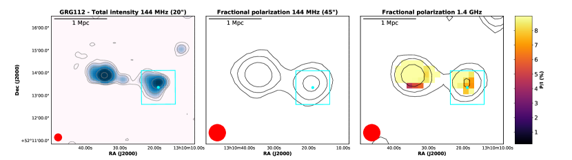
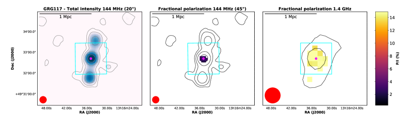
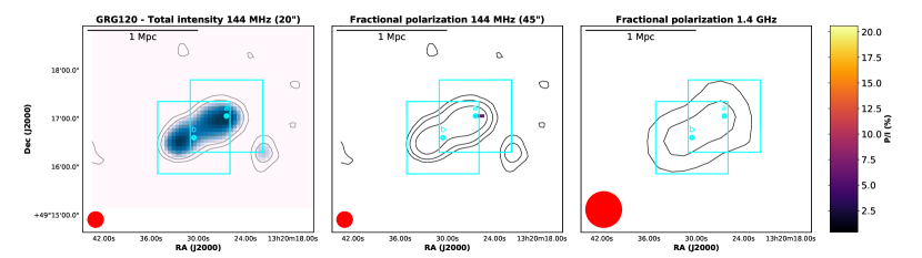
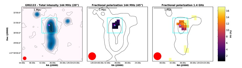
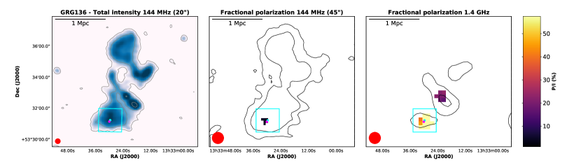
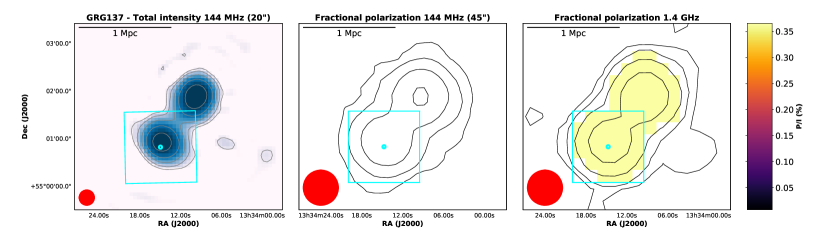
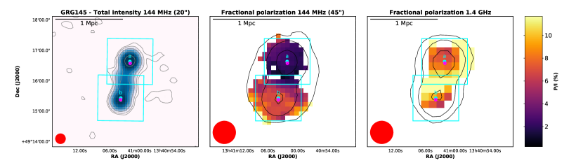
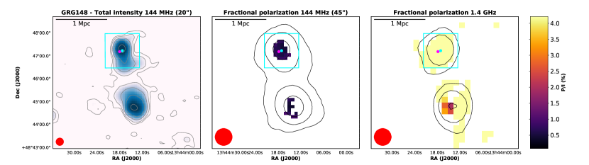
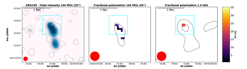
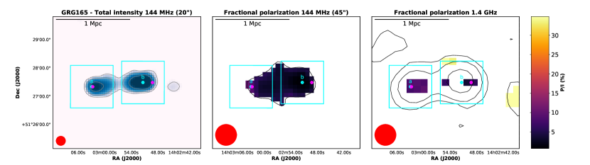
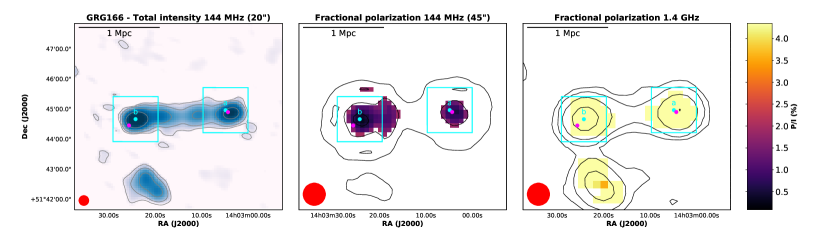
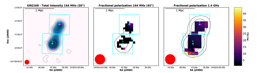
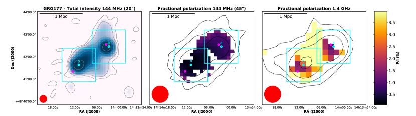
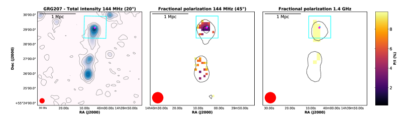
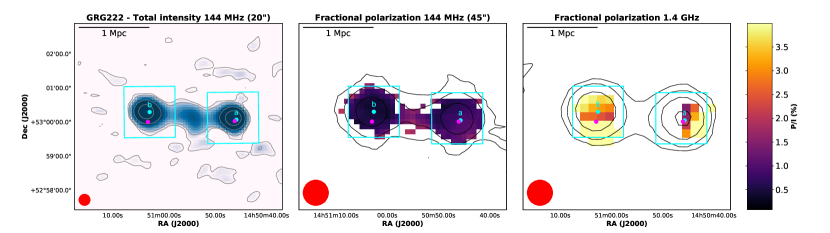
Figure A9 (continued):

Figure A9 (continued):

Figure A9 (continued):

Figure A9 (continued):

Figure A9 (continued):

Figure A9 (continued):

Figure A9 (continued):

Figure A9 (continued):

References

- Astropy Collaboration et al. (2013) Astropy Collaboration, Robitaille, T. P., Tollerud, E. J., et al. 2013, A&A, 558, A33
- Becker et al. (1995) Becker, R. H., White, R. L., & Helfand, D. J. 1995, ApJ, 450, 559
- Böhringer et al. (2016) Böhringer, H., Chon, G., & Kronberg, P. P. 2016, A&A, 596, A22
- Bonafede et al. (2010) Bonafede, A., Feretti, L., Murgia, M., et al. 2010, A&A, 513, A30
- Bonafede et al. (2011) Bonafede, A., Govoni, F., Feretti, L., et al. 2011, A&A, 530, A24
- Bonnarel et al. (2000) Bonnarel, F., Fernique, P., Bienaymé, O., et al. 2000, A&AS, 143, 33
- Brentjens (2018) Brentjens, M. A. 2018, Astrophysics and Space Science Library, Vol. 426, Polarization Imaging with LOFAR, 159
- Brentjens & de Bruyn (2005) Brentjens, M. A. & de Bruyn, A. G. 2005, A&A, 441, 1217
- Bridle et al. (1979) Bridle, A. H., Davis, M. M., Fomalont, E. B., Willis, A. G., & Strom, R. G. 1979, ApJ, 228, L9
- Brüggen et al. (2005) Brüggen, M., Ruszkowski, M., Simionescu, A., Hoeft, M., & Dalla Vecchia, C. 2005, ApJ, 631, L21
- Burn (1966) Burn, B. J. 1966, MNRAS, 133, 67
- Cavaliere & Fusco-Femiano (1976) Cavaliere, A. & Fusco-Femiano, R. 1976, A&A, 500, 95
- Chen et al. (2011) Chen, R., Peng, B., Strom, R. G., & Wei, J. 2011, MNRAS, 412, 2433
- Clarke (2004) Clarke, T. E. 2004, Journal of Korean Astronomical Society, 37, 337
- Clarke et al. (2001) Clarke, T. E., Kronberg, P. P., & Böhringer, H. 2001, ApJ, 547, L111
- Condon et al. (1998) Condon, J. J., Cotton, W. D., Greisen, E. W., et al. 1998, AJ, 115, 1693
- Dabhade et al. (2017) Dabhade, P., Gaikwad, M., Bagchi, J., et al. 2017, MNRAS, 469, 2886
- Dabhade et al. (2020) Dabhade, P., Röttgering, H. J. A., Bagchi, J., et al. 2020, A&A, 635, A5
- Davé et al. (2001) Davé, R., Cen, R., Ostriker, J. P., et al. 2001, ApJ, 552, 473
- Dolag et al. (2001) Dolag, K., Schindler, S., Govoni, F., & Feretti, L. 2001, A&A, 378, 777
- Duncan et al. (2019) Duncan, K. J., Sabater, J., Röttgering, H. J. A., et al. 2019, A&A, 622, A3
- Fanaroff & Riley (1974) Fanaroff, B. L. & Riley, J. M. 1974, MNRAS, 167, 31P
- Farnsworth et al. (2011) Farnsworth, D., Rudnick, L., & Brown, S. 2011, AJ, 141, 191
- Felten (1996) Felten, J. E. 1996, Astronomical Society of the Pacific Conference Series, Vol. 88, Mitigating the Baryon Crisis in Clusters: Can Magnetic Pressure be Important?, ed. V. Trimble & A. Reisenegger, 271
- Garrington et al. (1988) Garrington, S. T., Leahy, J. P., Conway, R. G., & Laing, R. A. 1988, Nature, 331, 147
- George et al. (2012) George, S. J., Stil, J. M., & Keller, B. W. 2012, Publications of the Astronomical Society of Australia, 29, 214
- Govoni et al. (2017) Govoni, F., Murgia, M., Vacca, V., et al. 2017, A&A, 603, A122
- Hales et al. (2012) Hales, C. A., Gaensler, B. M., Norris, R. P., & Middelberg, E. 2012, MNRAS, 424, 2160
- Hao et al. (2010) Hao, J., McKay, T. A., Koester, B. P., et al. 2010, ApJS, 191, 254
- Heald (2009) Heald, G. 2009, in IAU Symposium, Vol. 259, Cosmic Magnetic Fields: From Planets, to Stars and Galaxies, ed. K. G. Strassmeier, A. G. Kosovichev, & J. E. Beckman, 591–602
- Hill et al. (1996) Hill, G. J., Goodrich, R. W., & Depoy, D. L. 1996, ApJ, 462, 163
- Hunter (2007) Hunter, J. D. 2007, Computing in Science and Engineering, 9, 90
- Ishwara-Chandra & Saikia (1999) Ishwara-Chandra, C. H. & Saikia, D. J. 1999, MNRAS, 309, 100
- Johnson et al. (1995) Johnson, R. A., Leahy, J. P., & Garrington, S. T. 1995, MNRAS, 273, 877
- Johnston-Hollitt & Ekers (2004) Johnston-Hollitt, M. & Ekers, R. D. 2004, arXiv e-prints, astro
- Joye & Mandel (2003) Joye, W. A. & Mandel, E. 2003, Astronomical Society of the Pacific Conference Series, Vol. 295, New Features of SAOImage DS9, ed. H. E. Payne, R. I. Jedrzejewski, & R. N. Hook, 489
- Kuźmicz et al. (2018) Kuźmicz, A., Jamrozy, M., Bronarska, K., Janda-Boczar, K., & Saikia, D. J. 2018, ApJS, 238, 9
- Laing (1988) Laing, R. A. 1988, Nature, 331, 149
- Laing et al. (2006) Laing, R. A., Canvin, J. R., Cotton, W. D., & Bridle, A. H. 2006, MNRAS, 368, 48
- Laing et al. (1983) Laing, R. A., Riley, J. M., & Longair, M. S. 1983, MNRAS, 204, 151
- Lawler & Dennison (1982) Lawler, J. M. & Dennison, B. 1982, ApJ, 252, 81
- Machalski & Jamrozy (2006) Machalski, J. & Jamrozy, M. 2006, A&A, 454, 95
- Mack et al. (1997) Mack, K. H., Klein, U., O’Dea, C. P., & Willis, A. G. 1997, A&AS, 123, 423
- Mack et al. (1998) Mack, K. H., Klein, U., O’Dea, C. P., Willis, A. G., & Saripalli, L. 1998, A&A, 329, 431
- Mahatma et al. (2019) Mahatma, V. H., Hardcastle, M. J., Williams, W. L., et al. 2019, A&A, 622, A13
- Malarecki et al. (2015) Malarecki, J. M., Jones, D. H., Saripalli, L., Staveley-Smith, L., & Subrahmanyan, R. 2015, MNRAS, 449, 955
- Mevius (2018) Mevius, M. 2018, RMextract: Ionospheric Faraday Rotation calculator
- Mulcahy et al. (2014) Mulcahy, D. D., Horneffer, A., Beck, R., et al. 2014, A&A, 568, A74
- Murgia et al. (2004) Murgia, M., Govoni, F., Feretti, L., et al. 2004, A&A, 424, 429
- Neld et al. (2018) Neld, A., Horellou, C., Mulcahy, D. D., et al. 2018, A&A, 617, A136
- Offringa et al. (2014) Offringa, A. R., McKinley, B., Hurley-Walker, et al. 2014, MNRAS, 444, 606
- Oppermann et al. (2015) Oppermann, N., Junklewitz, H., Greiner, M., et al. 2015, A&A, 575, A118
- Orrù et al. (2015) Orrù, E., van Velzen, S., Pizzo, R. F., et al. 2015, A&A, 584, A112
- O’Sullivan et al. (2018a) O’Sullivan, S., Brüggen, M., Van Eck, C., et al. 2018a, Galaxies, 6, 126
- O’Sullivan et al. (2020) O’Sullivan, S. P., Brüggen, M., Vazza, F., et al. 2020, arXiv e-prints, arXiv:2002.06924
- O’Sullivan et al. (2018b) O’Sullivan, S. P., Lenc, E., Anderson, C. S., Gaensler, B. M., & Murphy, T. 2018b, MNRAS, 475, 4263
- O’Sullivan et al. (2019) O’Sullivan, S. P., Machalski, J., Van Eck, C. L., et al. 2019, A&A, 622, A16
- Peng et al. (2015) Peng, B., Chen, R. R., & Strom, R. 2015, in Advancing Astrophysics with the Square Kilometre Array (AASKA14), 109
- Planck Collaboration et al. (2016) Planck Collaboration, Ade, P. A. R., Aghanim, N., et al. 2016, A&A, 594, A27
- Pshirkov et al. (2015) Pshirkov, M. S., Tinyakov, P. G., & Urban, F. R. 2015, MNRAS, 452, 2851
- Robitaille & Bressert (2012) Robitaille, T. & Bressert, E. 2012, APLpy: Astronomical Plotting Library in Python
- Rudnick (2019) Rudnick, L. 2019, arXiv e-prints, arXiv:1901.09074
- Schnitzeler (2010) Schnitzeler, D. H. F. M. 2010, MNRAS, 409, L99
- Shimwell et al. (2017) Shimwell, T. W., Röttgering, H. J. A., Best, P. N., et al. 2017, A&A, 598, A104
- Shimwell et al. (2019) Shimwell, T. W., Tasse, C., Hardcastle, M. J., et al. 2019, A&A, 622, A1
- Shulevski et al. (2019) Shulevski, A., Barthel, P. D., Morganti, R., et al. 2019, A&A, 628, A69
- Simonetti et al. (1984) Simonetti, J. H., Cordes, J. M., & Spangler, S. R. 1984, ApJ, 284, 126
- Sokoloff et al. (1998) Sokoloff, D. D., Bykov, A. A., Shukurov, A., et al. 1998, MNRAS, 299, 189
- Sotomayor-Beltran et al. (2013) Sotomayor-Beltran, C., Sobey, C., Hessels, J. W. T., et al. 2013, A&A, 552, A58
- Stil et al. (2011) Stil, J. M., Taylor, A. R., & Sunstrum, C. 2011, ApJ, 726, 4
- Strom & Jaegers (1988) Strom, R. G. & Jaegers, W. J. 1988, A&A, 194, 79
- Stuardi et al. (2019) Stuardi, C., Bonafede, A., Wittor, D., et al. 2019, MNRAS, 489, 3905
- Subrahmanyan et al. (2008) Subrahmanyan, R., Saripalli, L., Safouris, V., & Hunstead, R. W. 2008, ApJ, 677, 63
- Sun & Han (2004) Sun, X. H. & Han, J. L. 2004, in The Magnetized Interstellar Medium, ed. B. Uyaniker, W. Reich, & R. Wielebinski, 25–30
- Tasse (2014) Tasse, C. 2014, A&A, 566, A127
- Tasse et al. (2018) Tasse, C., Hugo, B., Mirmont, M., et al. 2018, A&A, 611, A87
- Taylor et al. (2009) Taylor, A. R., Stil, J. M., & Sunstrum, C. 2009, ApJ, 702, 1230
- Taylor (2005) Taylor, M. B. 2005, Astronomical Society of the Pacific Conference Series, Vol. 347, TOPCAT & STIL: Starlink Table/VOTable Processing Software, ed. P. Shopbell, M. Britton, & R. Ebert, 29
- Tribble (1991) Tribble, P. C. 1991, MNRAS, 250, 726
- Tsien (1982) Tsien, S. C. 1982, MNRAS, 200, 377
- Van Eck (2018) Van Eck, C. 2018, Galaxies, 6, 112
- Van Eck et al. (2019) Van Eck, C. L., Haverkorn, M., Alves, M. I. R., et al. 2019, A&A, 623, A71
- Van Eck et al. (2018) Van Eck, C. L., Haverkorn, M., Alves, M. I. R., et al. 2018, A&A, 613, A58
- van Weeren et al. (2016) van Weeren, R. J., Williams, W. L., Hardcastle, M. J., et al. 2016, ApJS, 223, 2
- Vazza et al. (2017) Vazza, F., Brüggen, M., Gheller, C., et al. 2017, Classical and Quantum Gravity, 34, 234001
- Vazza et al. (2019) Vazza, F., Ettori, S., Roncarelli, M., et al. 2019, A&A, 627, A5
- Vernstrom et al. (2019) Vernstrom, T., Gaensler, B. M., Rudnick, L., & Andernach, H. 2019, ApJ, 878, 92
- Wen & Han (2015) Wen, Z. L. & Han, J. L. 2015, ApJ, 807, 178
- Wen et al. (2012) Wen, Z. L., Han, J. L., & Liu, F. S. 2012, ApJS, 199, 34
- Williams et al. (2019) Williams, W. L., Hardcastle, M. J., Best, P. N., et al. 2019, A&A, 622, A2
- Williams et al. (2016) Williams, W. L., van Weeren, R. J., Röttgering, H. J. A., et al. 2016, MNRAS, 460, 2385
- Willis et al. (1974) Willis, A. G., Strom, R. G., & Wilson, A. S. 1974, Nature, 250, 625
- Willis et al. (1978a) Willis, A. G., Wilson, A. S., & Strom, R. G. 1978a, A&A, 66, L1
- Willis et al. (1978b) Willis, A. G., Wilson, A. S., & Strom, R. G. 1978b, A&A, 66, L1
- Wright (2006) Wright, E. L. 2006, Publications of the Astronomical Society of the Pacific, 118, 1711
- York et al. (2000) York, D. G., Adelman, J., Anderson, John E., J., et al. 2000, AJ, 120, 1579