QCD Odderon: non linear evolution in the leading twist

Abstract

In the paper we propose and solve analytically the non-linear evolution equation in the leading twist approximation for the Odderon contribution. We found three qualitative features of this solution, which differs the Odderon contribution from the Pomeron one :(i) the behaviour in the vicinity of the saturation scale cannot be derived from the linear evolution in a dramatic difference with the Pomeron case; (ii) a substantial decrease of the Odderon contribution with the energy; and (iii) the lack of geometric scaling behaviour. The two last features have been seen in numerical attempts to solve the Odderon equation.

I Introduction

The new data of the TOTEM collaborationTOTEMRHO1 ; TOTEMRHO2 ; TOTEMRHO3 ; TOTEMRHO4 triggered hot discussions on the Odderon: a state with negative signature and with an intercept, which is close to unity (see Refs.KMRO ; BJRS ; TT ; MN ; BLM ; SS ; KMRO1 ; KMRO2 ; GLP ; CNPSS ). This state arises naturally in perturbative QCD (see Ref.KOLEB for the review). In Refs.BLV ; KS the linear equation for the perturbative Odderon has been derived and it has been shown, that the intercept of the Odderon is equal $\alpha_{\rm Odd}\left(t=0\right)\,\,=\,\,1$. Having negative signature such an Odderon generates the real part of the scattering amplitude, which does not depend on energy. Specifically such an Odderon has been discussed in the phenomenological attempts to describe the experimental data in Refs. KMRO ; BJRS ; TT ; MN ; BLM ; SS ; KMRO1 ; KMRO2 ; GLP ; CNPSS .

However, in the Colour Glass Condensate(CGC) approach, the energy dependence of the Odderon contribution is affected by the shadowing correctionsKS ; KOLEB , which result in a decrease of the Odderon amplitude with increasing energy. In this paper, we wish to discuss the non-linear evolution of the Odderon in the CGC approach continuing research started by Refs.KS ; KOLEB .

We wish to recall that CGC approach is the only candidate for the effective theory at high energies, which is based on our microscopic theory: QCD (see Ref.KOLEB for a review). It has been shown that the non linear equations for the positive signature (Balitsky-Kovchegov (BK) equationsBK ) take a simple form, if we use the simplified BFKL kernelBFKL and restrict ourselves to the contribution of the leading twist only. In this paper we generalize this approach for the case of the Odderon contribution.

II Balitsky-Kovchegov(BK) equation in the leading twist approximation

The BK evolution equation for the dipole-target scattering amplitude $N\left(\boldsymbol{x}_{10},\boldsymbol{b},Y;R\right)$ has the general form in the leading order (LO) of perturbative QCD ($R$ denotes the size of the target)KOLEB ; BK ; GLR ; MUQI ; MV :

$$\frac{\partial}{\partial Y}N\left(\boldsymbol{x}_{10},\boldsymbol{b},Y;R\right)=$$ (1)

$$\bar{\alpha}_{S}\!\!\int\frac{d^{2}\boldsymbol{x}_{2}}{2\,\pi}\,K\left(\boldsymbol{x}_{02},\boldsymbol{x}_{12};\boldsymbol{x}_{10}\right)\Bigg{(}N\left(\boldsymbol{x}_{12},\boldsymbol{b}-\frac{1}{2}\boldsymbol{x}_{20},Y;R\right)+N\left(\boldsymbol{x}_{20},\boldsymbol{b}-\frac{1}{2}\boldsymbol{x}_{12},Y;R\right)-N\left(\boldsymbol{x}_{10},\boldsymbol{b},Y;R\right)$$

$$-\,\,N\left(\boldsymbol{x}_{12},\boldsymbol{b}-\frac{1}{2}\boldsymbol{x}_{20},Y;R\right)\,N\left(\boldsymbol{x}_{20},\boldsymbol{b}-\frac{1}{2}\boldsymbol{x}_{12},Y;R\right)\Bigg{)}$$ (2)

where $\boldsymbol{x}_{ik}\,\,=\,\,\boldsymbol{x}_{i}\,-\,\boldsymbol{x}_{k}$ and $\boldsymbol{x}_{10}\equiv\,\boldsymbol{r}$, $\boldsymbol{x}_{20}\,\equiv\,\boldsymbol{r}^{\prime}$ and $\boldsymbol{x}_{12}\,\equiv\,\boldsymbol{r}\,-\,\boldsymbol{r}^{\prime}$. $Y$ is the rapidity of the scattering dipole and $\boldsymbol{b}$ is the impact factor. $K\left(\boldsymbol{x}_{02},\boldsymbol{x}_{12};\boldsymbol{x}_{10}\right)$ is the kernel of the BFKL equation which in the leading order has the following form:

$$K^{\rm LO}\left(\boldsymbol{x}_{02},\boldsymbol{x}_{12};\boldsymbol{x}_{10}\right)\,\,=\,\,\frac{x^{2}_{10}}{x^{2}_{02}\,x^{2}_{12}}$$ (3)

For the kernel of the LO BFKL equation (see Eq. (3)) the eigenvalues take the formBFKL ; LIP :

$$\omega\left(\bar{\alpha}_{S},\gamma\right)\,\,=\,\,\bar{\alpha}_{S}\,\chi^{LO}\left(\gamma\right)\,\,\,=\,\,\,\bar{\alpha}_{S}\left(2\psi\left(1\right)\,-\,\psi\left(\gamma\right)\,-\,\psi\left(1-\gamma\right)\right)$$ (4)

where $\psi(z)$ is the Euler psi-function $\psi\left(z\right)=d\ln\Gamma(z)/dz$. The general BFKL kernel of Eq. (3) and Eq. (4) has contributions of all possible twists, and it cannot be solved analytically. However, as it was shown in Ref.LETU the situation becomes much simpler if we restrict ourselves to the leading twist contribution to the BFKL kernel, which has the formLETU

$$\chi\left(\gamma\right)\,\,=\,\,\left\{\begin{array}[]{l}\,\,\,\frac{1}{\gamma}\,\,\,\,\,\,\,\,\,\,\mbox{for}\,\,\,\tau\,=\,rQ_{s}\,>\,1\,\,\,\,\,\,\mbox{summing}\left(\ln\left(rQ_{s}\right)\right)^{n};\\ \\ \,\,\,\frac{1}{1\,-\,\gamma}\,\,\,\,\,\mbox{for}\,\,\,\tau\,=\,rQ_{s}\,<\,1\,\,\,\,\,\mbox{summing}\left(\ln\left(1/(r\,\Lambda_{\rm QCD})\right)\right)^{n};\\ \end{array}\right.$$ (8)

instead of the full expression of Eq. (4).

In the saturation region where $\tau\,\,>\,\,1$ the logs originate from the decay of a large size dipole into one small size dipole and one large size dipoleLETU . However, the size of the small dipole is still larger than $1/Q_{s}$. This observation can be translated to the following form of the kernel in the LO

$$\frac{\bar{\alpha}_{S}}{2\pi}\int\,\displaystyle{K\left(\boldsymbol{x}_{01};\boldsymbol{x}_{02},\boldsymbol{x}_{12}\right)}\,d^{2}x_{02}\, \rightarrow \,\frac{\bar{\alpha}_{S}}{2}\,\int^{x^{2}_{01}}_{1/Q^{2}_{s}(Y,b)}\frac{dx^{2}_{02}}{x_{02}^{2}}\,\,+\,\,\frac{\bar{\alpha}_{S}}{2}\,\int^{x^{2}_{01}}_{1/Q^{2}_{s}(Y,b)}\frac{d|\boldsymbol{x}_{01}-\boldsymbol{x}_{02}|^{2}}{|\boldsymbol{x}_{01}-\boldsymbol{x}_{02}|^{2}}\,\,$$ (9)

$$= \,\,\frac{\bar{\alpha}_{S}}{2}\,\int^{\xi}_{\xi_{s}}d\xi_{02}\,\,+\,\,\frac{\bar{\alpha}_{S}}{2}\,\int^{\xi}_{\xi_{s}}d\xi_{12}$$

where $\xi_{ik}\,=\,\ln\left(x^{2}_{ik}Q_{s}^{2}(Y=Y_{0})\right)$.

Inside the saturation region the BK equation in LO, takes the form

$$\frac{\partial^{2}\widetilde{N}\left(Y;\xi,\boldsymbol{b}\right)}{\partial Y\,\partial\xi}\,\,=\,\,\bar{\alpha}_{S}\,\left\{\left(1\,\,-\,\frac{\partial\widetilde{N}\left(Y;\xi,\boldsymbol{b}\right)}{\partial\xi}\right)\,\widetilde{N}\left(Y;\xi,\boldsymbol{b}\right)\right\}$$ (10)

where $\widetilde{N}\left(Y;\xi,\boldsymbol{b}\right)\,\,=\,\,\int^{\xi}_{\ln Q^{2}_{s}(Y)}d\xi^{\prime}\,N\left(Y;\xi^{\prime},\boldsymbol{b}\right)$ .

Introducing

$$N\left(Y;\xi^{\prime},\boldsymbol{b}\right)\,\,=\,\,1\,\,-\,\,\Delta\left(Y;\xi^{\prime},\boldsymbol{b}\right)\,\,=\,\,1\,\,-\,\,e^{-\Omega\left(Y;\xi^{\prime},\boldsymbol{b}\right)}$$ (11)

we can reduce Eq. (10) to the following expressions:

$$\frac{\partial\,\Omega\left(Y;\xi^{\prime},\boldsymbol{b}\right)}{\partial\,Y}\,\,=\,\,\bar{\alpha}_{S}\,\,\widetilde{N}\left(Y;\xi,\boldsymbol{b}\right);~{}~{}~{}~{}~{}~{}~{}~{}\frac{\partial^{2}\,\Omega\left(Y;\xi^{\prime},\boldsymbol{b}\right)}{\partial\,Y\,\,\partial\,\xi}\,\,=\,\,\bar{\alpha}_{S}\,\Bigg{(}1\,\,-\,\,e^{-\,\Omega\left(Y;\xi^{\prime},\boldsymbol{b}\right)}\Bigg{)}$$ (12)

Looking for the traveling wave solution (geometric scalingBALE ; MUT ; IIML ; SGBK ) , we assume that $\Omega\left(Y;\xi^{\prime},\boldsymbol{b}\right)\,\,\equiv\,\,\Omega\left(z\right)$ with

$$z\,\,=\,\,\ln\tau\,\,=\,\,\ln\left(Q^{2}_{s}\left(Y,b\right)\,r^{2}\right)\,\,=\,\,4\,\bar{\alpha}_{S}\,Y\,\,+\,\,\xi$$ (13)

Eq. (12) takes the form:

$$\frac{d^{2}\,\Omega\left(z\right)}{d\,z^{2}}\,\,=\,\,\frac{1}{4}\,\Bigg{(}1\,\,-\,\,e^{-\,\Omega\left(z\right)}\Bigg{)}$$ (14)

which has the solution (see formula 3.4.1.1 of Ref.MATH ):

$$\sqrt{2}\int^{\Omega}_{\Omega_{0}}\,d\Omega^{\prime}\,\,\frac{1}{\sqrt{\Omega^{\prime}\,\,+\,\,e^{-\Omega^{\prime}}\,\,-\,\,1\,\,+\,\,{\rm C}}}\,\,=\,\,z$$ (15)

for the function $\Omega$.

The value of $C$ has to be determined from matching with the region $\tau\,<\,1$. For small $\Omega_{0}$   $C=0$. Indeed, in this case the solution at small $\Omega$ has the following form:

$$\Omega\,\,=\,\,\Omega_{0}\,e^{\frac{1}{2}\,z}$$ (16)

which coincides with the general solutionMUT for the region $\tau\,<\,1$ at small $\Omega_{0}\,=\,N_{0}\,\ll\,1$.

III Linear evolution in perturbative QCD region

III.1 The BFKL equation

The linear equation for the Odderon is the same as the BFKL equation, which takes the form:

$$\frac{\partial}{\partial Y}O\left(\boldsymbol{x}_{10},\boldsymbol{b},Y;R\right)=\bar{\alpha}_{S}\!\!\int\frac{d^{2}\boldsymbol{x}_{2}}{2\,\pi}\,K\left(\boldsymbol{x}_{02},\boldsymbol{x}_{12};\boldsymbol{x}_{10}\right)\Bigg{\{}O\left(\boldsymbol{x}_{12},\boldsymbol{b}-\frac{1}{2}\boldsymbol{x}_{20},Y;R\right)+O\left(\boldsymbol{x}_{20},\boldsymbol{b}-\frac{1}{2}\boldsymbol{x}_{12},Y;R\right)-O\left(\boldsymbol{x}_{10},\boldsymbol{b},Y;R\right)\Bigg{\}}$$ (17)

Therefore, the difference between the BFKL Pomeron and Odderon stems from the initial conditions and the signature: positive for the BFKL Pomeron and negative for the Odderon. As it is shown in Ref.LIP ; KS the general solution to Eq. (17) can be written as

$$O\left(\boldsymbol{x}_{10},\boldsymbol{b},\boldsymbol{x}_{1^{\prime}0^{\prime}};Y\right)\,\,=\,\,c_{0}\bar{\alpha}_{S}^{3}\frac{6}{\pi^{3}}\sum^{\infty}_{k=0}\int^{\infty+i\epsilon}_{-\infty+i\epsilon}\!\!\!\!\!\!d\nu\,e^{\omega\left(\bar{\alpha}_{S},k,\nu\right)\,Y}\,\chi\left(k,\nu\right)\,\frac{\nu^{2}+\frac{(2k+1)^{2}}{4}}{(\nu^{2}+k^{2})\,(\nu^{2}\,+\,(k+1)^{2})}G_{\nu,k}\left(\boldsymbol{\rho}_{1},\boldsymbol{\rho}_{0},\boldsymbol{\rho}_{1^{\prime}},\boldsymbol{\rho}_{0^{\prime}}\right)$$ (18)

where the eigenvalues $\omega\left(\bar{\alpha}_{S},k,\nu\right)$ are equal to LIP

$$\omega\left(\bar{\alpha}_{S},k,\nu\right)\,\,\,=\,\,\,\bar{\alpha}_{S}\,\chi\left(k,\nu\right)\,\,\, = \bar{\alpha}_{S}\Big{(}2\,\psi(1)\,-\,\psi(\frac{1+|n|}{2}\,+\,i\nu)\,-\,\psi(\frac{1+|n|}{2}\,-\,i\nu)\Big{)}$$

$$\left(|n|\,=\,2\,k\,+\,1\right) = \,\,\,\bar{\alpha}_{S}\Big{(}2\,\psi(1)\,-\,\psi(k\,+\,1\,+\,i\nu)\,-\,\psi(k\,+\,1\,-\,i\nu)\Big{)}$$ (19)

and the eigenfunctions have the following formLIP ; NAPE :

$$G_{\nu,k}\left(\boldsymbol{\rho}_{1},\boldsymbol{\rho}_{0},\boldsymbol{\rho}_{1^{\prime}},\boldsymbol{\rho}_{0^{\prime}}\right)\,\,=\,\,c_{1}\,w^{h}\,w^{*\tilde{h}}{}_{2}F_{3}\left(h,h,2\,h,w\right)\,\,+\,\,c_{2}\,w^{1-h}\,w^{*1-\tilde{h}}{}_{2}F_{3}\left(1-\tilde{h},1-\tilde{h},2\,-2\,\tilde{h},w^{*}\right)$$ (20)

where ${}_{2}F_{3}$ denotes the hypergeometric function (see formula 9.1 in Ref.RY ),

$$w\,\,=\,\,\frac{\rho_{01}\,\rho_{0^{\prime}1^{\prime}}}{\rho_{00^{\prime}}\,\rho_{11^{\prime}}};~{}~{}~{}~{}\,\,h\,=\,k\,+\,1\,+\,i\,\nu;~{}~{}~{}\,\,\,\tilde{h}\,=\,\,\,-\,k\,\,+\,\,i\,\nu;$$ (21)

and

$$c_{2}\,=\,\frac{b_{k,\nu}}{2\,\pi^{2}};~{}~{}~{}\frac{c_{1}}{c_{2}}\,=\,\frac{b_{k,-\nu}}{b_{k,\nu}};~{}~{}~{}b_{k,\nu}\,\,=\,\,\pi^{3}\,2^{4\,i\,\nu}\frac{\Gamma\left(-i\nu\,+\,k+1\right)\,\Gamma\left(i\,\nu\,+k\,+\,\frac{1}{2}\right)}{\Gamma\left(i\,\nu\,+\,k\,+\,1\right)\,\Gamma\left(-i\,\nu\,+k+\frac{1}{2}\right)}$$ (22)

We characterize all two dimensional vectors, shown in Fig. 1, by complex numbers, specifically

$$\rho_{k}\,=\,x_{k}+i\,y_{k};~{}~{}~{}~{}\rho^{*}_{k}\,=\,=\,x_{k}-i\,y_{k};~{}~{}~{}\boldsymbol{\rho}_{k}\,=\,(x_{k},y_{k});$$ (23)

Eq. (18) differs from the solution for the BFKL Pomeron, since the sum in this equation is over odd $n=2\,k+1$, while in the case of the BFKL Pomeron we sum over even $n\,=\,2\,k$. Indeed, the Odderon corresponds to the negative signature which generates the states that change sign under charge conjugation, which, as was shown in Ref.KS corresponds to replacing quark $\boldsymbol{x}_{1}$ by anti-quark $\boldsymbol{x}_{0}$, or in other words $\boldsymbol{x}_{01}\,\to\,-\boldsymbol{x}_{01}$. Since eigenfunctions under this transformation have the following properties:

$$G_{\nu,k}\left(\boldsymbol{x}_{01},\boldsymbol{x}_{0^{\prime}1^{\prime}},\boldsymbol{b}\right)\,\,=\,\,\left(-1\right)^{n}\,G_{\nu,k}\left(-\,\boldsymbol{x}_{01},\boldsymbol{x}_{0^{\prime}1^{\prime}},\boldsymbol{b}\right)$$ (24)

we see that the Pomeron and Odderon correspond to summation over even and odd $n$, respectively.

Figure 1: The initial condition for evolution of the Odderon: the three gluon exchange in Born Approximation of perturbative QCD.

Eq. (18) satisfies the initial condition, which is given by the Born Approximation diagram of Fig. 1KS :

$$O_{0}\left(\boldsymbol{x}_{0},\boldsymbol{x}_{1};Y=0\right)\,\,=\,\,c_{0}\bar{\alpha}_{S}^{3}\,\ln^{3}\left(w\,w^{*}\right);~{}~{}~{}~{}~{}~{}~{}~{}~{}c_{0}\,\,=\,\,\frac{(N_{c}^{2}-4)\,(N^{2}_{c}-1)}{4\,N^{3}_{c}}$$ (25)

where $N_{c}$ denotes the number of colours.

The main contribution in sum of Eq. (18), stems from $k=0$. $\omega\left(k=0,\nu\right)$ is shown in Fig. 2-a. One can see that the maximal intercept is equal to 0. At $Y\,\gg\,Y_{0}$ the main contribution to Eq. (18), gives the term with $k$=0 and, hence, the Odderon contribution for $w\,w^{*}\,\ll\,1$ takes the form :

$$O\left(\boldsymbol{x}_{10},\boldsymbol{b},Y;\boldsymbol{x}_{1^{\prime}0^{\prime}};Y\right)\,\,=$$ (26)

$$\,\,c_{0}\bar{\alpha}_{S}^{3}\frac{6}{\pi^{3}}\,\int^{\infty+i\epsilon}_{-\infty+i\epsilon}\!\!\!\!\!\!d\nu\,e^{\omega\left(\bar{\alpha}_{S},0,\nu\right)\,Y}\,\chi\left(0,\nu\right)\,\frac{\nu^{2}+\frac{1}{4}}{(\nu^{2})\,(\nu^{2}\,+\,1)}\Bigg{\{}c_{1}\left(\frac{w}{w^{*}}\right)^{\frac{1}{2}}\left(w\,w^{*}\right)^{\frac{1}{2}+i\,\nu}\,\,+\,\,c_{2}\left(\frac{w}{w^{*}}\right)^{-\frac{1}{2}}\left(w\,w^{*}\right)^{\frac{1}{2}-i\,\nu}\Bigg{\}}$$

$$=c_{0}\bar{\alpha}_{S}^{3}\frac{6}{\pi^{3}}\,\int^{\infty+i\epsilon}_{-\infty+i\epsilon}\!\!\!\!\!\!d\nu\,e^{\omega\left(\bar{\alpha}_{S},0,\nu\right)\,Y}\,\chi\left(0,\nu\right)\,\frac{\nu^{2}+\frac{1}{4}}{(\nu^{2})\,(\nu^{2}\,+\,1)}\Bigg{\{}c_{1}\left(\frac{w}{w^{*}}\right)^{\frac{1}{2}}e^{\left(\frac{1}{2}+i\,\nu\right)\,\xi}\,\,+\,\,c_{2}\left(\frac{w}{w^{*}}\right)^{-\frac{1}{2}}e^{\left(\frac{1}{2}-i\,\nu\right)\,\xi}\Bigg{\}}$$

with

$$w\,w^{*}\,\,=\,\,\frac{r^{2}\,R^{2}}{\left(\boldsymbol{b}+\frac{1}{2}(\boldsymbol{r}-\boldsymbol{R})\right)^{2}\,\left(\boldsymbol{b}-\frac{1}{2}(\boldsymbol{r}-\boldsymbol{R})\right)^{2}}\,\,\equiv\,\,e^{\xi}$$ (27)

where $b$ denotes the impact parameter of two colliding dipoles with sizes $r$ and $R$ (see Fig. 1).

Fig. 2-a		Fig. 2-b

Figure 2: Fig. 2-a: $\omega\left(\bar{\alpha}_{S},k=0,\nu\right)$ versus $\nu$. The red line shows $\omega=0$.Fig. 2-b: The singular behaviour of $\omega\left(\bar{\alpha}_{S},k=0,\nu\right)$ versus $\gamma$, where $\gamma\,\equiv\,i\,\nu$.

III.2 Diffusion approximation

We can evaluate the integral of Eq. (26) using the expansion of $\chi\left(0,\nu\right)$ with respect to $\nu$. Specifically,

$$\chi\left(k=0,\nu\right)\,\,=\,\,-\,D\,\nu^{2}\,\,=\,\,\,-\,2\,\zeta\left(3\right)\nu^{2}\,\,+\,\,{\cal O}\left(\nu^{3}\right)$$ (28)

where $\zeta\left(3\right)$ is the Riemann $\zeta$ function ($\zeta\left(3\right)\,\approx\,1.2$)RY .

Using the method of steepest descent we see that Eq. (28) leads to the following estimates for Eq. (26):

$$O\left(\boldsymbol{x}_{10},\boldsymbol{b},Y;\boldsymbol{x}_{1^{\prime}0^{\prime}};Y\right)\,\,=\,\,c_{0}\bar{\alpha}_{S}^{3}\frac{3}{\pi^{3/2}}\,\sqrt{\frac{D}{2\,Y}}e^{-\frac{\xi^{2}}{4\,\bar{\alpha}_{S}\,D\,\,Y}}\,\left(c_{1}\,w\,+\,c_{2}\,w^{*}\right)$$ (29)

Therefore, the $\xi$ and $Y$ dependence for the Odderon look similar to the BFKL Pomeron in the diffusion approximation(see Ref.KOLEB ), but the value of $D$ for the Odderon in 7 times smaller than for the Pomeron.

III.3 Double Log Approximation(DLA ) in coordinate representation

In Fig. 2-b we plot the dependence of the eigenvalues $\omega\left(\bar{\alpha}_{S},k=0,\gamma\right)$ versus $\gamma\,=\,i\,\nu$. This eigenvalue has two singularities at $\gamma\,=\,\pm 1$. In the vicinities of these points $\omega\left(\bar{\alpha}_{S},k=0,\gamma\right)\,\,\propto\frac{\bar{\alpha}_{S}}{1\pm\gamma}$. From past experience with the BFKL Pomeron we expect that such singularities generate the double log contributions. We can see this explicitly by re-writing Eq. (26) in the new notation

$$\left(w\,w^{*}\right)^{\gamma}\,=\,e^{\gamma\xi}\,=\,e^{-\gamma\xi^{\prime}}=\,e^{\left(1\,-\,\gamma\right)\xi^{\prime}\,\,-\,\,\xi^{\prime}}$$

with $\xi^{\prime}\,=\,-\xi\,\,=\,\,\ln\left(\frac{1}{w\,w^{*}}\right)\,>\,0$ for small dipole size $r\,\,\ll\,\,R\,\leq\,b$. With the new variables the contribution of the first term of Eq. (26) takes the form:

$$O^{\rm DLA}\left(\xi;Y\right)\,\, = \,\,\,\,c_{0}\bar{\alpha}_{S}^{3}\frac{12}{\pi^{2}}\,\int^{\epsilon+i\infty}_{\epsilon-i\infty}\!\!\!\!\frac{d\gamma}{2\,i\,\pi}\,e^{\frac{\bar{\alpha}_{S}}{1-\gamma}\,Y\,\,+\,\,\left(1-\gamma\right)\,\xi^{\prime}}\,\Bigg{\{}\chi\left(0,\gamma\right)\,\frac{-\gamma^{2}+\frac{1}{4}}{(-\gamma^{2})\,(-\gamma^{2}\,+\,1)}c_{1}(\gamma)\Bigg{\}}\Big{(}ww\,w^{*}\Big{)}$$ (30)

$$= \,\,c_{0}\bar{\alpha}_{S}^{3}\frac{12}{\pi^{2}}\,\int^{\epsilon+i\infty}_{\epsilon-i\infty}\!\!\!\!\frac{d\gamma}{2\,i\,\pi}\,\sum_{n=0}^{\infty}\left(\frac{\bar{\alpha}_{S}Y}{1-\gamma}\right)^{n}e^{\,\,\left(1-\gamma\right)\,\xi^{\prime}}\,\Bigg{\{}\chi\left(0,\gamma\right)\,\frac{-\gamma^{2}+\frac{1}{4}}{(-\gamma^{2})\,(-\gamma^{2}\,+\,1)}c_{1}(\gamma)\Bigg{\}}\Big{(}ww\,w^{*}\Big{)}$$

$$= {\rm Const}\,\sum_{n=0}^{\infty}\frac{\left(\bar{\alpha}_{S}\,Y\,\xi^{\prime}\right)^{n}}{\left(n!\right)^{2}}\Big{(}ww\,w^{*}\Big{)}\,\,\,\equiv\,\,\Big{(}ww\,w^{*}\Big{)}\,o\left(\bar{\alpha}_{S}\,Y\,\xi^{\prime}\right)$$

where in ${\rm Const}$ we absorbed all constant factors. Deriving the last equation we use that $\Big{\{}\dots\Big{\}}\xrightarrow{\gamma\to 1}\frac{1}{1-\gamma}$. It is easy to show that the second term has the contribution which can be written in the form: $\Big{(}w^{*}w\,w^{*}\Big{)}\,o\left(\bar{\alpha}_{S}\,Y\,\xi^{\prime}\right)$.

Generally the DLA contribution occurs in the form:

$$O^{\rm DLA}\left(\xi;Y\right)\,\,=\,\,\left(w\,+\,w^{*}\right)w\,w^{*}\,o^{\rm DLA}\left(\bar{\alpha}_{S}\,Y\,\xi^{\prime}\right)$$ (31)

The same structure can be seen directly from Eq. (17). Indeed, the DL contribution stems from the sizes $x_{02}\,\sim\,x_{12}\,\gg\,x_{10}$. In this kinematic region the BFKL kernel has a simple form (see Eq. (3)

$$K^{\rm LO}\left(\boldsymbol{x}_{02},\boldsymbol{x}_{12};\boldsymbol{x}_{10}\right)\,\,\xrightarrow{x_{02}\,\sim\,x_{12}\,\gg\,x_{10}}\,\,x^{2}_{10}\Bigg{\{}\frac{1}{x_{02}^{4}}\,\,+\,\,\frac{2\boldsymbol{x}_{01}\cdot\boldsymbol{x}_{02}}{x_{02}^{6}}\Bigg{\}}\,\,=\,\,x^{2}_{10}\Bigg{\{}\frac{1}{x_{02}^{4}}\,\,+\,\,2\,\frac{x_{10}}{x_{02}^{5}}\,\cos\varphi\Bigg{\}}$$ (32)

where $\varphi$ denotes the angle between vectors $\boldsymbol{x}_{10}$ and $\boldsymbol{x}_{02}$.

Plugging this kernel in Eq. (17) we see that Eq. (17) takes the form:

$$\frac{\partial}{\partial Y}O^{\rm DLA}\left(\xi^{\prime},Y\right)=\bar{\alpha}_{S}\!\!\int\frac{d^{2}\boldsymbol{x}_{02}}{2\,\pi}\,\,x^{2}_{10}\Bigg{\{}\frac{1}{x_{02}^{4}}\,\,+\,\,2\,\frac{x_{10}}{x_{02}^{5}}\,\cos\varphi\Bigg{\}}\,O^{\rm DLA}\left(\xi^{\prime\prime};Y\right)$$ (33)

Recalling that $w\,w^{*}\,\,\propto\,\,x^{2}_{02}$ and that Eq. (31) can be re-written as follows:

$$O^{\rm DLA}\left(\xi";Y\right)\,\,=\,\,\cos\varphi(w\,w^{*})^{3/2}\,o^{\rm DLA}\left(\bar{\alpha}_{S}\,Y\,\xi^{\prime\prime}\right)$$ (34)

one can see that the first term in Eq. (33) vanishes due to integration over $\varphi$ and the second term can be re-written as

$$\frac{\partial}{\partial Y}\,o^{\rm DLA}\left(\xi^{\prime},Y\right)\,\,=\,\,\bar{\alpha}_{S}\,\int^{\xi^{\prime}}\!\!\!\!\!\!\,d\xi^{\prime\prime}\,o^{\rm DLA}\left(\xi^{\prime\prime};Y\right)$$ (35)

III.4 Geometric scaling behaviour of the scattering amplitude in the vicinity of the saturation momentum

It is well knownKOLEB ; GLR ; BALE ; LETU ; IIML ; MUT , that for finding the saturation momentum, as well as for discussing the behaviour of the scattering amplitude in the vicinity of the saturation scale, we do not need to know the precise structure of the non-linear corrections. What we need, is to find the solution of the linear BFKL equation, which is a wave package that satisfies the condition, that phase and group velocities are equalGLR . In other words, we need to take the integral in Eq. (26) by the method of steepest descend, and to satisfy two conditions for the saddle point ($\nu_{\rm sp}$):

$$(1)~{}~{}\frac{d\,\omega\left(\bar{\alpha}_{S},0,\nu_{\rm sp}\right)}{d\nu_{\rm sp}}\,Y\,\,+\,i\,\xi\,\,=\,\,0;~{}~{}~{}~{}(2)~{}~{}\omega\left(\bar{\alpha}_{S},0,\nu_{\rm sp}\right)\,Y\,\,+\,\,\left(\frac{1}{2}+i\,\nu_{\rm sp}\right)\,\xi\,\,=\,\,0$$ (36)

The first equation determines the trajectory of the wave package, while the second fixes the front line on which our wave function is a constant. Dividing one equation by the second one, we obtain the following equation, which actually gives $v_{\rm group}\,=\,v_{\rm phase}$:

$$\frac{d\,\omega\left(\bar{\alpha}_{S},0,\nu_{\rm sp}\right)}{d\nu_{\rm sp}}\,\,=\,\,v_{\rm group}\,\,=\,\,v_{\rm phase}\,\,=\,\,\,\,i\,\frac{\omega\left(\bar{\alpha}_{S},0,\nu_{\rm sp}\right)}{\frac{1}{2}+i\,\nu_{\rm sp}}$$ (37)

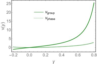
Figure 3: Eq. (37): $v_{\rm group}$ and $v_{\rm phase}$ versus $\gamma\equiv\,i\,\nu$.

In Fig. 3 we plot the l.h.s. and the r.h.s. Eq. (37). One can see that this equation has no solution except at $\gamma=0$. However, at $\gamma\to 0$ $v_{\rm group}\,\propto\,\gamma^{2}$ while $v_{\rm phase}\,\propto\,\gamma$ and, therefore, Eq. (37) does not have solution at small $\gamma$.

This can be seen directly from Eq. (29) . At first sight the diffusion solution of Eq. (29) is constant for $\xi$ determined from the following equation:

$$-\frac{\xi^{2}}{4\,\bar{\alpha}_{S}\,D\,Y}\,+\,\xi\,\,=\,\,0$$ (38)

For $R\,\gg\,r,b$ $\xi=\,\ln\left(r^{2}/R^{2}\right)\,<\,0$. One can see that Eq. (38) has no solution for negative $\xi$. Recall, that in section III-B we found the saddle point, but without an additional condition of Eq. (36)-2.

Hence, the situation with the Odderon turns out to be quite different from the BFKL Pomeron: the linear equation does not provide saturation, which might or might not stem from the solution to the non-linear equation, that was derived in Ref.KS (see also Ref.KOLEB ). We also see no reason for the geometric scaling behaviour for the Odderon contribution. However, there is still the possibility that the non-linear evolution will lead to a geometric scaling solution, with the saturation scale determined by Eq. (10).

IV Non-linear evolution for the Odderon

IV.1 General equation

The non-linear evolution equation for the Odderon is derived in Ref.KS (see also Ref.KOLEB ). It takes the form:

$$\frac{\partial}{\partial Y}O\left(\boldsymbol{x}_{10},\boldsymbol{b},Y;R\right)=$$ (39)

$$\bar{\alpha}_{S}\!\!\int\frac{d^{2}\boldsymbol{x}_{2}}{2\,\pi}\,K\left(\boldsymbol{x}_{02},\boldsymbol{x}_{12};\boldsymbol{x}_{10}\right)\Bigg{\{}O\left(\boldsymbol{x}_{12},\boldsymbol{b}-\frac{1}{2}\boldsymbol{x}_{20},Y;R\right)+O\left(\boldsymbol{x}_{20},\boldsymbol{b}-\frac{1}{2}\boldsymbol{x}_{12},Y;R\right)-\,\,O\left(\boldsymbol{x}_{01},\boldsymbol{b},Y;R\right)\,$$

$$-\,\,N\left(\boldsymbol{x}_{20},\boldsymbol{b}-\frac{1}{2}\boldsymbol{x}_{12},Y;R\right)\,O\left(\boldsymbol{x}_{12},\boldsymbol{b}-\frac{1}{2}\boldsymbol{x}_{20},Y;R\right)\,\,-\,\,N\left(\boldsymbol{x}_{12},\boldsymbol{b}-\frac{1}{2}\boldsymbol{x}_{20},Y;R\right)\,O\left(\boldsymbol{x}_{20},\boldsymbol{b}-\frac{1}{2}\boldsymbol{x}_{12},Y;R\right)\Bigg{\}}$$

where the amplitude $N$ is the solution of the BK equation (see Eq. (1)) for the Pomeron.

$$N\left(\boldsymbol{x}_{01},\boldsymbol{b},Y;R\right)\,\,=\,\,1\,\,-\,\,\Delta\left(\boldsymbol{x}_{01},\boldsymbol{b},Y;R\right)\,\,=\,\,1\,\,-\,\,\exp\left(-\Omega\left(\boldsymbol{x}_{01},\boldsymbol{b},Y;R\right)\right)$$ (40)

We can re-write Eq. (39) in the form:

$$\frac{\partial}{\partial Y}O\left(\boldsymbol{x}_{10},\boldsymbol{b},Y;R\right)\,\,=\,\,\bar{\alpha}_{S}\!\!\int\frac{d^{2}\boldsymbol{x}_{2}}{2\,\pi}\,K\left(\boldsymbol{x}_{02},\boldsymbol{x}_{12};\boldsymbol{x}_{10}\right)\Bigg{\{}-\,\,O\left(\boldsymbol{x}_{01},\boldsymbol{b},Y;R\right)\,\,$$ (41)

$$+\,\,\Delta\left(\boldsymbol{x}_{20},\boldsymbol{b}-\frac{1}{2}\boldsymbol{x}_{12},Y;R\right)\,O\left(\boldsymbol{x}_{12},\boldsymbol{b}-\frac{1}{2}\boldsymbol{x}_{20},Y;R\right)\,\,+\,\,\Delta\left(\boldsymbol{x}_{12},\boldsymbol{b}-\frac{1}{2}\boldsymbol{x}_{20},Y;R\right)\,O\left(\boldsymbol{x}_{20},\boldsymbol{b}-\frac{1}{2}\boldsymbol{x}_{12},Y;R\right)\Bigg{\}}$$

As we have discussed in section II function $\Delta\left(z\right)$ depends on one variable $z\,\,=\,\,\ln\left(r^{2}\,Q^{2}_{s}\left(Y,b\right)\right)$, where $Q_{s}$ is the saturation momentum determined by the Baltsky-Kovchegov equation (see Eq. (1)). As one can see from Fig. 4, the function $\Delta$ decreases at large $z$ and is peaked at $z=0$.

Fig. 4-a		Fig. 4-b

Figure 4: Fig. 4-a: Functions $\Delta\left(z\right)$ and $\Omega\left(z\right)$ from Eq. (15) for $\Omega_{0}(z=0)=0.2$. Fig. 4-b: Function $Z(z)$ from Eq. (47) in which $\Omega(z)$ is calculated from Eq. (15) with $\Omega_{0}=0.2$.

IV.2 Equation in the leading twist approximation

Using Eq. (9) for the BFKL kernel in the leading twist approximation, we we can reduce Eq. (39) to the following equation:

$$\frac{\partial}{\partial Y}\,O\left(\boldsymbol{x}_{10},\boldsymbol{b},Y;R\right)\,\,=\,\,-\bar{\alpha}_{S}\!\!\int^{x^{2}_{01}}_{1/Q^{2}_{s}}\frac{dx^{2}_{02}}{x^{2}_{02}}\,\,O\left(\boldsymbol{x}_{01},\boldsymbol{b},Y;R\right)\,\,$$ (42)

$$+\,\,\bar{\alpha}_{S}\,\Delta\left(\boldsymbol{x}_{01},\boldsymbol{b},Y;R\right)\,\int^{x^{2}_{01}}_{1/Q^{2}_{s}}\frac{dx^{2}_{02}}{x^{2}_{02}}\,\,O\left(\boldsymbol{x}_{02},\boldsymbol{b},Y;R\right)\,\,+\,\,\bar{\alpha}_{S}\,\int^{x^{2}_{01}}_{1/Q^{2}_{s}}\frac{dx^{2}_{02}}{x^{2}_{02}}\,\,\Delta\left(\boldsymbol{x}_{02},\boldsymbol{b},Y;R\right)\,O\left(\boldsymbol{x}_{01},\boldsymbol{b},Y;R\right)$$

Looking for the solution in the form

$$O\left(\boldsymbol{x}_{10},\boldsymbol{b},Y;R\right)\,\,=\,\,o\left(\boldsymbol{x}_{10},\boldsymbol{b},Y;R\right)\,e^{-\Omega\left(z\right)}$$ (43)

we obtain the following equation for $o\left(\boldsymbol{x}_{10},\boldsymbol{b},Y;R\right)$:

$$\frac{\partial}{\partial Y}\,o\left(\xi,Y\right)\,\,-\,\,\frac{d\,\Omega\left(z\right)}{dY}\,o\left(\xi,Y\right)=\,\,-\bar{\alpha}_{S}\,z\,o\left(\xi,Y\right)\,\,+\,\,\bar{\alpha}_{S}\,\,\int^{\xi}d\,\xi^{\prime}\,\,o\left(\xi^{\prime},Y\right)\,e^{-\Omega\left(z\right)}\,\,+\,\,\bar{\alpha}_{S}\,\int^{z}d\,z^{\prime}\,\,\Delta\left(z^{\prime}\right)\,o\left(\xi,Y\right)$$ (44)

where $\xi$ is defined by Eq. (27). The first equation of Eq. (12) can be rewritten in the form:

$$\frac{\partial}{\partial Y}\,\Omega\left(z\right)\,\,=\,\,\bar{\alpha}_{S}\left(\,z\,\,-\,\,\,\int^{z}d\,z^{\prime}\,\,\Delta\left(z^{\prime}\right)\right)$$ (45)

Plugging this equation into Eq. (44) we reduce it to the form:

$$\frac{\partial}{\partial Y}\,o\left(\xi,Y\right)\,\,\,=\,\,\,\bar{\alpha}_{S}\,\,\int^{\xi}d\,\xi^{\prime}\,\,o\left(\xi^{\prime},Y\right)\,e^{-\Omega\left(z^{\prime}\right)};~{}~{}~{}~{}~{}~{}~{}~{}~{}\frac{\partial^{2}}{\partial Y\,\partial\,\xi}\,o\left(\xi,Y\right)\,\,\,=\,\,\,\bar{\alpha}_{S}e^{-\,\Omega\left(z\right)}\,o\left(\xi,Y\right)$$ (46)

Introducing a new variable

$$Z\,\,\,=\,\,\,\int^{z}_{0}\!\!\!d\,z^{\prime}\,e^{-\,\Omega\left(z^{\prime}\right)}$$ (47)

we re-write the equation as follows:

$$\frac{\partial^{2}}{\partial{Z}\,\partial\,\xi}\,o\left(\xi,{Z}\right)\,\,=\,\,\frac{1}{4}\,o\left(\xi,{Z}\right)$$ (48)

IV.3 Solution

The solution to Eq. (48) takes the general form:

$$o\left(\xi,{Z}\right)\,\,\,=\,\,\,\int^{\epsilon\,+\,i\,\infty}_{\epsilon\,-\,i\,\infty}\frac{d\,\gamma}{2\,\pi\,i}e^{\frac{1}{4}\frac{1}{\gamma}\,Z\,\,+\,\,\gamma\xi}\,\tilde{o}\left(\gamma\right)$$ (49)

where $\tilde{o}\left(\gamma\right)$ should be found from the initial condition at $z=0$($Z=0$). We need to solve Eq. (35) to find this initial condition. Its solution has the form:

$$O^{\rm DLA}\left(\xi^{\prime};Y\right)\,\,=\,\,\frac{w}{w^{*}}\,O_{0}\int^{\epsilon\,+\,i\,\infty}_{\epsilon\,-\,i\,\infty}\frac{d\,\gamma}{2\,\pi\,i}\,e^{\frac{\bar{\alpha}_{S}}{\gamma}\,Y\,\,+\,\,\gamma\xi^{\prime}-\frac{3}{2}\xi^{\prime}}\,\frac{1}{\gamma}$$ (50)

with the initial condition $O^{\rm DLA}\left(\xi^{\prime};Y=0\right)\,\,=\,\,\frac{w}{w^{*}}\,\left(w\,w^{*}\right)^{3/2}\,O_{0}$, where $O_{0}$ is a constant. On the line $z=0$ Eq. (50) gives

$$O^{\rm DLA}\left(\xi^{\prime};z=0\left(4\bar{\alpha}_{S}Y=\xi^{\prime}\right)\right)\,\,=\,\,\,O_{0}\int^{\epsilon\,+\,i\,\infty}_{\epsilon\,-\,i\,\infty}\frac{d\,\gamma}{2\,\pi\,i}\,e^{\frac{1}{4}\frac{1}{\gamma}\,\xi^{\prime}\,\,+\,\,\gamma\xi^{\prime}-\frac{3}{2}\xi^{\prime}}\,\frac{1}{\gamma}$$ (51)

Taking into account Eq. (43) we obtain the following initial condition for $o\left(\xi,{Z}\right)$:

$$o\left(\xi,Z=0\right)\,\,\,=\,\,\,\int^{\epsilon\,+\,i\,\infty}_{\epsilon\,-\,i\,\infty}\frac{d\,\gamma}{2\,\pi\,i}e^{\gamma\xi}\,\tilde{o}\left(\gamma\right)\,\,=\,\,\,O_{0}\,e^{\Omega_{0}}\int^{\epsilon\,+\,i\,\infty}_{\epsilon\,-\,i\,\infty}\frac{d\,\gamma}{2\,\pi\,i}\,e^{\frac{1}{4}\frac{1}{\gamma}\,\xi^{\prime}\,\,+\,\,\gamma\xi^{\prime}-\frac{3}{2}\xi^{\prime}}\,\frac{1}{\gamma}$$ (52)

The r.h.s. of this equation we can re-write as

$$O_{0}\,e^{\Omega_{0}}\int^{\epsilon\,+\,i\,\infty}_{\epsilon\,-\,i\,\infty}\frac{d\,\gamma^{\prime}}{2\,\pi\,i}\,\frac{d\gamma(\gamma^{\prime})}{d\,\gamma^{\prime}}\,e^{\gamma^{\prime}\xi}\,\frac{1}{\gamma(\gamma^{\prime})}$$ (53)

where $\gamma(\gamma^{\prime})$ is the solution top the following equation:

$$\frac{1}{4}\frac{1}{\gamma}\,\,\,+\,\,\gamma-\frac{3}{2}=-\,\gamma^{\prime}$$ (54)

The solution to this equation gives:

$$\gamma_{\pm}(\gamma^{\prime})\,\,=\,\,\frac{1}{2}\Bigg{(}\frac{3}{2}\,-\,\gamma^{\prime}\,\pm\,\sqrt{\left(\gamma^{\prime}-\frac{1}{2}\right)\,\left(\gamma^{\prime}-\frac{5}{2}\right)}\Bigg{)}$$ (55)

Plugging Eq. (55) into Eq. (53) we obtain

$$\tilde{o}\left(\gamma\right)\,\,=\,\,\,O_{0}\,e^{\Omega_{0}}\,\frac{1}{\sqrt{\left(\gamma-\frac{1}{2}\right)\,\left(\gamma-\frac{5}{2}\right)}}$$ (56)

Hence the solution takes the form:

$$o\left(\xi,{Z}\right)\,\,\,=\,\,\,\,O_{0}\,e^{\Omega_{0}}\,\int^{\epsilon\,+\,i\,\infty}_{\epsilon\,-\,i\,\infty}\frac{d\,\gamma}{2\,\pi\,i}e^{\frac{1}{4}\frac{1}{\gamma}\,Z\,\,+\,\,\gamma\xi}\,\frac{1}{\sqrt{\left(\gamma-\frac{1}{2}\right)\,\left(\gamma-\frac{5}{2}\right)}}$$ (57)

For large $z$ and $\xi$, we can evaluate this integral using the method of steepest descend. For the saddle point we have the following equation:

$$-\frac{Z}{4\,\gamma^{2}_{\rm sp}}\,\,+\,\,\xi\,\,=\,\,0;~{}~{}~{}~{}~{}\gamma_{\rm sp}\,\,=\,\,\frac{1}{2}\sqrt{\frac{Z}{\xi}}\,\,\ll\,1\,\,\mbox{for}\,\,\,\xi\,\,\gg\,\,1$$ (58)

From Eq. (58) we obtain the solution:

$$o\left(\xi,Z\right)\,\,\,=\,\,\,\,O_{0}\,e^{\Omega_{0}}\,\sqrt{\pi}\frac{\gamma^{3}_{\rm sp}}{4\,Z}\frac{2}{\sqrt{5}}\,e^{\sqrt{Z\,\xi}}$$ (59)

which leads to the Odderon contribution

$$O\left(\xi,Z\right)\,\,\,=\,\,\,\frac{w}{w^{*}}\,O_{0}\,e^{\Omega_{0}\,-\,\Omega\left(z\right)}\,\sqrt{\pi}\frac{\gamma^{3}_{\rm sp}}{2\,Z}\,e^{\sqrt{Z\,\xi}}$$ (60)

In Fig. 5 solutions of Eq. (60) are plotted as a function of $z$ at fixed $\xi$. One can see that all solutions lead to the Odderon contribution which is negligibly small at $z\,\geq 5$.

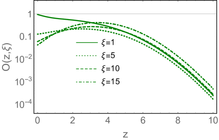
Figure 5: Solution for $O\left(\xi,Z\right)$ of Eq. (60) versus $z$ at fixed $\xi$. $\Omega_{0}$=0.2, $O_{0}$=0.2.

V Conclusions

In the paper we proposed and solved analytically the non-linear evolution equation in the leading twist approximation for the Odderon contribution. We found three qualitative features of this solution, where the Odderon contribution differs from the Pomeron one: (i ) the behaviour in the vicinity of the saturation scale cannot be derived from the linear evolution in a dramatic difference with the Pomeron case; (ii) the substantial decrease of the Odderon contribution with the energy; and (iii) the lack of the geometric scaling behaviour. All of these features can be see from Fig. 5 and Eq. (60). The decrease of the Odderon contribution with energy should be confronted with the QCD linear equation prediction for the intercept of the Odderon: $\alpha_{\rm Odd}\left(t=0\right)\,=\,1$, which means that the Odderon contribution does not depend on energy. The geometric scaling behaviour is the most striking general feature of the non-linear Balitsky-Kovchegov equationLETU ; BALE ; IIML ; SGBK . Therefore, the Odderon provides an example that this behaviour is the characteristic property of the Pomeron contributions. It is instructive to mention, that in spite of the violation of the geometric scaling behaviour for the Odderon, the suppression deep in the saturation region is the same as for the Pomeron case, and is determined by the gluon reggeization LETU . We would like to stress that some of these features( the decrease with energy and the lack of the geometric scaling behaviour) have been seen in the numerical solutions to the non-linear evolution of the QCD OdderonLRRW ; YHH ; and the decrease of the Odderon contribution with energy follows from the general non-linear equationKS ; KOLEB , using the approach of Ref.LETU .

Concluding we wish to stress that the QCD Odderon gives a very small contribution to the scattering amplitude, due to substantial shadowing corrections, which are responsible for the non-linear evolution. We believe that this solid theoretical result based on the effective QCD theory at high energy: the CGC approach, will be useful in our discussion of the available experimental data.

VI Acknowledgements

We thank our colleagues at Tel Aviv university and UTFSM for encouraging discussions. Our special thanks go Errol Gotsman for his everyday advices and discussions on the subject of the paper. We wish to thank Yoshitaka Hatta, who drew our attention to the numerical solutions for the QCD Odderon, that we overlooked.

This research was supported by Proyecto Basal FB 0821(Chile), Fondecyt (Chile) grants 1180118 and 1191434.

References

• (1) G. Antchev et al. [TOTEM Collaboration], “First measurement of elastic, inelastic and total cross-section at $\sqrt{s}=13$ TeV by TOTEM and overview of cross-section data at LHC energies,” Eur. Phys. J. C 79 (2019) no.2, 103 doi:10.1140/epjc/s10052-019-6567-0 [arXiv:1712.06153 [hep-ex]].
• (2) G. Antchev et al. [TOTEM Collaboration], “First determination of the ${\rho}$ parameter at ${\sqrt{s}=13}$ TeV: probing the existence of a colourless C-odd three-gluon compound state,” Eur. Phys. J. C 79 (2019) no.9, 785 doi:10.1140/epjc/s10052-019-7223-4 [arXiv:1812.04732 [hep-ex]].
• (3) G. Antchev et al. [TOTEM Collaboration], “Elastic differential cross-section measurement at $\sqrt{s}=13$ TeV by TOTEM,” Eur. Phys. J. C 79 (2019) no.10, 861 doi:10.1140/epjc/s10052-019-7346-7 [arXiv:1812.08283 [hep-ex]].
• (4) G. Antchev et al. [TOTEM Collaboration], “Elastic differential cross-section ${\mathrm{d}}\sigma/{\mathrm{d}}t$ at $\sqrt{s}=2.76\hbox{ TeV}$ and implications on the existence of a colourless C-odd three-gluon compound state,” Eur. Phys. J. C 80 (2020) no.2, 91 doi:10.1140/epjc/s10052-020-7654-y [arXiv:1812.08610 [hep-ex]].
• (5) V. A. Khoze, A. D. Martin and M. G. Ryskin, “Elastic and diffractive scattering at the LHC,” arXiv:1806.05970 [hep-ph].
• (6) W. Broniowski, L. Jenkovszky, E. Ruiz Arriola and I. Szanyi, “Hollowness in $pp$ and $p\bar{p}$ scattering in a Regge model,” arXiv:1806.04756 [hep-ph].
• (7) S. M. Troshin and N. E. Tyurin, “Implications of the $\rho(s)$ measurements by TOTEM at the LHC,” arXiv:1805.05161 [hep-ph].
• (8) E. Martynov and B. Nicolescu, “Evidence for maximality of strong interactions from LHC forward data,” arXiv:1804.10139 [hep-ph].
• (9) M. Broilo, E. G. S. Luna and M. J. Menon, “Soft Pomerons and the Forward LHC Data,” Phys. Lett. B 781 (2018) 616, [arXiv:1803.07167 [hep-ph]].
• (10) Y. M. Shabelski and A. G. Shuvaev, ‘Real part of $pp$ scattering amplitude in Additive Quark Model at LHC energies,” Eur. Phys. J. C 78 (2018) no.6, 497, [arXiv:1802.02812 [hep-ph]].
• (11) V. A. Khoze, A. D. Martin and M. G. Ryskin, “Black disk, maximal Odderon and unitarity,” Phys. Lett. B 780 (2018) 352, [arXiv:1801.07065 [hep-ph]].
• (12) V. A. Khoze, A. D. Martin and M. G. Ryskin, “Elastic proton-proton scattering at 13 TeV,” Phys. Rev. D 97 (2018) no.3, 034019, [arXiv:1712.00325 [hep-ph]].
• (13) E. Gotsman, E. Levin and I. Potashnikova, “CGC/saturation approach: secondary Reggeons and $\rho={\rm Re/Im}$ dependence on energy,” Phys. Lett. B 786 (2018) 472 doi:10.1016/j.physletb.2018.10.017 [arXiv:1807.06459 [hep-ph]].
• (14) T. Csörgő,   T.  Novak, R.Pasechnik, A. Ster and I. Szanyi, “Evidence of Odderon-exchange from scaling properties of elastic scattering at TeV energies,” arXiv:1912.11968 [hep-ph].
• (15) Yuri V Kovchegov and Eugene Levin, “ Quantum Choromodynamics at High Energies", Cambridge Monographs on Particle Physics, Nuclear Physics and Cosmology, Cambridge University Press, 2012 .
• (16) J. Bartels, L. N. Lipatov and G. P. Vacca, “A New odderon solution in perturbative QCD,” Phys. Lett. B 477 (2000) 178, [hep-ph/9912423].
• (17) Y. V. Kovchegov, L. Szymanowski and S. Wallon, “Perturbative odderon in the dipole model,” Phys. Lett. B 586 (2004) 267, [hep-ph/0309281].
• (18) I. Balitsky, [arXiv:hep-ph/9509348];   Phys. Rev. D60, 014020 (1999) [arXiv:hep-ph/9812311];     Y. V. Kovchegov, Phys. Rev. D60, 034008 (1999), [arXiv:hep-ph/9901281].
• (19) V. S. Fadin, E. A. Kuraev and L. N. Lipatov, “On the pomeranchuk singularity in asymptotically free theories", Phys. Lett. B60, 50 (1975);    E. A. Kuraev, L. N. Lipatov and V. S. Fadin, “The Pomeranchuk Singularity in Nonabelian Gauge Theories" Sov. Phys. JETP 45, 199 (1977), [Zh. Eksp. Teor. Fiz.72,377(1977)];    I. I. Balitsky and L. N. Lipatov,“The Pomeranchuk Singularity in Quantum Chromodynamics,” Sov. J. Nucl. Phys. 28, 822 (1978), [Yad. Fiz.28,1597(1978)].
• (20) L. V. Gribov, E. M. Levin and M. G. Ryskin, “Semihard Processes in QCD,” Phys. Rept.  100 (1983) 1.
• (21) A. H. Mueller and J. Qiu, “Gluon recombination and shadowing at small values of $x$", Nucl. Phys. B268 (1986) 427
• (22) L. McLerran and R. Venugopalan, “Computing quark and gluon distribution functions for very large nuclei", Phys. Rev. D49 (1994) 2233, “Gluon distribution functions for very large nuclei at small transverse momentum", Phys. Rev. D49 (1994), 3352; ‘Green’s function in the color field of a large nucleus", D50 (1994) 2225; “ Fock space distributions, structure functions, higher twists, and small $x$" , D59 (1999) 09400.
• (23) L. N. Lipatov, “Small x physics in perturbative QCD,” Phys. Rept.  286 (1997) 131 doi:10.1016/S0370-1573(96)00045-2 [hep-ph/9610276];    “The Bare Pomeron in Quantum Chromodynamics,” Sov. Phys. JETP 63, 904 (1986) [Zh. Eksp. Teor. Fiz.  90, 1536 (1986)].
• (24) H.  Navelet and  R. B.Peschanski, R. B.Conformal invariance and the exact solution of BFKL equations, Nucl. Phys. B 507 353 (1997).
• (25) E. Levin and K. Tuchin, “Solution to the evolution equation for high parton density QCD,” Nucl. Phys. B 573, 833 (2000) [hep-ph/9908317];    “New scaling at high-energy DIS,” Nucl. Phys. A 691, 779 (2001) [hep-ph/0012167]; “Nonlinear evolution and saturation for heavy nuclei in DIS,” 693, 787 (2001) [hep-ph/0101275].
• (26) J. Bartels, E. Levin, “Solutions to the Gribov-Levin-Ryskin equation in the nonperturbative region,” Nucl. Phys.  B387 (1992) 617-637;
• (27) A. H. Mueller and D. N. Triantafyllopoulos, “The Energy dependence of the saturation momentum,” Nucl. Phys. B 640 (2002) 331 [hep-ph/0205167]
• (28) E. Iancu, K. Itakura and L. McLerran, “Geometric scaling above the saturation scale,” Nucl. Phys. A 708 (2002) 327 [hep-ph/0203137].
• (29) A. M. Stasto, K. J. Golec-Biernat, J. Kwiecinski, “Geometric scaling for the total gamma* p cross-section in the low x region,” Phys. Rev. Lett.  86 (2001) 596-599, [hep-ph/0007192].
• (30) A.D. Polyanin and V.F. Zaitsev “Handbook of nonlinear partial differential equations", Chapman and Hall/CRC Press, 2004, Raca Baton, New York, London, Tokyo
• (31) I. Gradstein and I. Ryzhik, Table of Integrals, Series, and Products, Fifth Edition, Academic Press, London, 1994.
• (32) T. Lappi, A. Ramnath, K. Rummukainen and H. Weigert, “JIMWLK evolution of the odderon,” Phys. Rev. D 94 (2016) no.5, 054014 doi:10.1103/PhysRevD.94.054014 [arXiv:1606.00551 [hep-ph]].
• (33) X. Yao, Y. Hagiwara and Y. Hatta, “Computing the gluon Sivers function at small-$x$,” Phys. Lett. B 790 (2019) 361 doi:10.1016/j.physletb.2019.01.029 [arXiv:1812.03959 [hep-ph]].