The Adaptive Stress Testing Formulation

Abstract

Validation is a key challenge in the search for safe autonomy. Simulations are often either too simple to provide robust validation, or too complex to tractably compute. Therefore, approximate validation methods are needed to tractably find failures without unsafe simplifications. This paper presents the theory behind one such black-box approach: adaptive stress testing (AST). We also provide three examples of validation problems formulated to work with AST.

I Introduction

An open question when robots operate autonomously in uncertain, real-world environments is how to tractably validate that the agent will act safely. Autonomous robotic systems may be expected to interact with a number of other actors, including humans, while handling uncertainty in perception, prediction and control. Consequently, scenarios are often too high-dimensional to tractably simulate in an exhaustive manner. As such, a common approach is to simplify the scenario by constraining the number of non-agent actors and the range of actions they can take. However, simulating simplified scenarios may compromise safety by eliminating the complexity needed to find rare, but important failures. Instead, approximate validation methods are needed to elicit agent failures while maintaining the full complexity of the simulation.

One possible approach to approximate validation is adaptive stress testing (AST) [7]. In AST, the validation problem is cast as a Markov decision process (MDP). A specific reward function structure is then used with reinforcement learning algorithms in order to identify the most-likely failure of a system in a scenario. Knowing the most-likely failure is useful for two reasons: 1) all other failures are at most as-likely, so it provides a bound on the likelihood of failures, and 2) it uncovers possible failure modes of an autonomous system so they can be addressed. AST is not a silver bullet: it requires accurate models of all actors in the scenario and is susceptible to local convergence. However, it allows failures to be identified tractably in simulation for complicated autonomous systems acting in high-dimensional spaces. This paper briefly presents the latest methodology for using AST and includes example validation scenarios formulated as AST problems.

II Methodology

II-A Adaptive Stress Testing

Adaptive stress testing formulates the problem of finding the most-likely failure of a system as a Markov decision process (MDP) [2]. Reinforcement learning (RL) algorithms can then be applied to efficiently find a solution in simulation. The process is shown in Figure 1. An RL-based solver outputs Environment Actions, which are the control input to the simulator. The simulator resolves the next time-step by executing the environment actions and then allowing the system-under-test (SUT) to act. The simulator returns the likelihood of the environment actions and whether an event of interest, such as a failure, has occurred. The reward function, covered in Section II-C, uses these to calculate the reward at each time-step. The solver uses these rewards to find the most-likely failure using reinforcement learning algorithms such as Monte Carlo tree search (MCTS) [4] or trust region policy optimization (TRPO) [10].

II-B Problem Formulation

Finding the most-likely failure of a system is a sequential decision-making problem. Given a simulator $\mathcal{S}$ and a subset of the state space $E$ where the events of interest (e.g. a collision) occur, we want to find the most-likely trajectory $s_{0},\ldots,s_{t}$ that ends in our subset $E$. Given $(\mathcal{S},E)$, the formal problem is

$$\underset{a_{0},\ldots,a_{t}}{\text{maximize}} P(s_{0},a_{0},\ldots,s_{t},a_{t})$$

subject to $$s_{t}\in E$$

where $P(s_{0},a_{0},\ldots,s_{t},a_{t})$ is the probability of a trajectory in simulator $\mathcal{S}$ and $s_{t}=f(a_{t},s_{t-1})$.

AST requires the following three functions to interact with the simulator:

• Initialize$(\mathcal{S},s_{0})$: Resets $\mathcal{S}$ to a given initial state $s_{0}$.

• Step$(\mathcal{S},E,a)$: Steps the simulation in time by drawing the next state $s^{\prime}$ after taking action $a$. The function returns the probability of the transition and an indicator showing whether $s^{\prime}$ is in $E$ or not.

• IsTerminal$(\mathcal{S},E)$: Returns true if the current state of the simulation is in $E$ or if the horizon of the simulation $T$ has been reached.

Figure 1: The AST methodology. The simulator is treated as a black box. The solver optimizes a reward based on transition likelihood and whether an event has occurred.

II-C Reward Function

In order to find the most-likely failure, the reward function must be structured as follows:

$$R\left(s\right)=\left\{\begin{array}[]{ll}0&s\in E\\ -\alpha-\beta f(s)&s\notin E,t\geq T\\ -g(a)-\eta h(s)&s\notin E,t<T\end{array}\right.$$ (1)

where the parameters are:

• $\alpha$: A large number, to heavily penalize trajectories that do not end in the target set.

• $\beta f(s)$: An optional heuristic. For example, in the autonomous vehicle experiment, we use the distance between the pedestrian and the car at the end of a trajectory. Consequently, the network takes actions that move the pedestrian close to the car early in training, allowing collisions to be found more quickly.

• $g(a)$: The action reward. A function recommended to be something proportional to $\log P(a)$. Adding log-probabilities is equivalent to multiplying probabilities and then taking the log, so this constraint ensures that summing the rewards from each time-step results in a total reward that is proportional to the log-probability of a trajectory.

• $\eta h(s)$: An optional training heuristic given at each timestep.

Looking at Equation 1, there are three cases:

• $s\in E$: The trajectory has terminated because an event has been found. This is the goal, so the reward at this step is as large as possible ($0\text{\,}\text{/}$).

• $s\notin E,t\geq T$: The trajectory has terminated by reaching the horizon $T$ without reaching an event. This is the least-useful outcome, so the user should set a large penalty.

• $s\notin E,t<T$: A time-step that was non-terminal, which is the most common case. The reward is generally proportional to the negative log-likelihood of the environment action, which promotes likely actions.

Ignoring heuristics for now, it is clear that the reward will be better for even a highly-unlikely trajectory that terminates in an event compared to a trajectory that fails to find an event. However, among trajectories that find an event, the more-likely trajectory will have a better reward. Consequently, optimizing to maximize reward will result in maximizing the probability of a trajectory that terminates with an event.

III Examples

We present three scenarios in which an autonomous system needs to be validated. For each scenario, we provide an example of how it could be formulated as an AST problem. Further details available in Appendix A.

III-A Cartpole with Disturbances

III-A1 Problem

Cartpole is a classic test environment for continuous control algorithms [1]. The system under test (SUT) is a neural network control policy trained by TRPO. The control policy controls the horizontal force $\vec{F}$ applied to the cart, and the goal is to prevent the bar on top of the cart from falling over.

III-A2 Formulation

We define an event as the pole reaching some maximum rotation or the cart reaching some maximum horizontal distance from the start position. The environment action is $\delta\vec{F}$, the disturbance force applied to the cart at each time-step. The reward function uses $\alpha=$1\text{\times}{10}^{4}\text{\,}\text{/}$$, $\beta=$1\text{\times}{10}^{3}\text{\,}\text{/}$$, and $f(s)$ as the normalized distance of the final state to failure states. The choice of $f(s)$ encourages the solver to push the SUT closer to failure. The action reward, $g(a)$ is set to the log of the probability density function of the natural disturbance force distribution. See Ma et al. [8].

III-B Autonomous Vehicle at a Crosswalk

III-B1 Problem

Autonomous vehicles must be able to safely interact with pedestrians. Consider an autonomous vehicle approaching a crosswalk on a neighborhood road. There is a single pedestrian who is free to move in any direction. The autonomous vehicle has imperfect sensors.

III-B2 Formulation

A collision between the car and pedestrian is the event we are looking for. The environment action vector controls both the motion of the pedestrian as well as the scale and direction of the sensor noise. The reward function for this scenario uses $\alpha=$-1\text{\times}{10}^{5}\text{\,}\text{/}$$ and $\beta=$-1\text{\times}{10}^{4}\text{\,}\text{/}$$, with $f(s)=\textsc{dist}\left(\boldsymbol{\mathbf{p}}_{v},\boldsymbol{\mathbf{p}}_{p}\right)$ as the distance between the pedestrian and the SUT at the end of a trajectory. This heuristic encourages the solver to move the pedestrian closer to the car in early iterations, which can significantly increase training speeds. The reward function also uses $g(a)=M\left(a,\mu_{a}\mid s\right)$, which is the Mahalanobis distance function [9]. Mahalanobis distance is a generalization of distance to the mean for multivariate distributions. See Koren et al. [5].

III-C Aircraft Collision Avoidance Software

III-C1 Problem

The next-generation Airborne Collision Avoidance System (ACASX) [3] gives instructions to pilots when multiple planes are approaching each other. We want to identify system failures in simulation to ensure the system is robust enough to replace the Traffic Alert and Collision Avoidance System (TCAS) [6]. We are interested in a number of different scenarios in which two or three planes are in the same airspace.

III-C2 Formulation

The event will be a near mid-air collision (NMAC), which is when two planes pass within 100 vertical feet and 500 horizontal feet of each other. The simulator is quite complicated, involving sensor, aircraft, and pilot models. Instead of trying to control everything explicitly, our environment actions will output seeds to the random number generators in the simulator. The reward function for this scenario uses $\alpha=\infty$ and no heuristics. The reward function also uses $g(a)=\log P(s_{t}\mid s_{t+1})$, the log of the known transition probability at each time-step. See Lee et al. [7].

IV Conclusion

This paper presents the latest formulation of adaptive stress testing, and examples of how it can be applied. AST is an approach to validation that can tractably find failures in autonomous systems in simulation without reducing scenario complexity. Autonomous systems are difficult to validate because they interact with many other actors in high-dimensional spaces according to complicated policies. However, validation is essential for producing autonomous systems that are safe, robust, and reliable.

Appendix A Examples: Further Details

A-A Cartpole with Disturbances

The cartpole scenario from Ma et al. [8] is shown in Figure 2. The state $s=[x,\dot{x},\theta,\dot{\theta}]$ represents the cart’s horizontal position and speed as well as the bar’s angle and angular velocity. The control policy, a neural network trained by TRPO, controls the horizontal force $\vec{F}$ applied to the cart. The failure of the system is defined as $|x|>x_{max}$ or $|\theta|>\theta_{max}$. The initial state is at $s_{0}=[0,0,0,0]$.

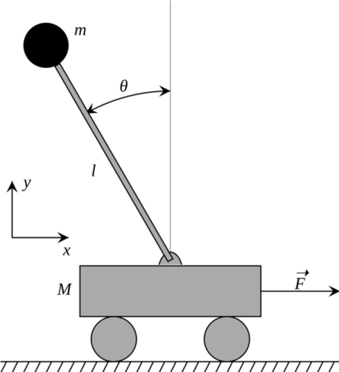
Figure 2: Layout of the cartpole environment. A control policy applies horizontal force on the cart to prevent the bar falling over.

A-B Autonomous Vehicle at a Crosswalk

The autonomous vehicle scenario from Koren et al. [5] is shown in Figure 3. The $x$-axis is aligned with the edge of the road, with East being the positive $x$-direction. The $y$-axis is aligned with the center of the cross-walk, with North being the positive $y$-direction. The pedestrian is crossing from South to North. The vehicle starts $35\text{\,}\mathrm{m}\text{/}$ from the crosswalk, with an initial velocity of $11.2\text{\,}\mathrm{m}\text{/}\mathrm{s}$ East. The pedestrian starts $2\text{\,}\mathrm{m}\text{/}$ away, with an initial velocity of $1\text{\,}\mathrm{m}\text{/}\mathrm{s}$ North. The autonomous vehicle policy is a modified version of the intelligent driver model [11].

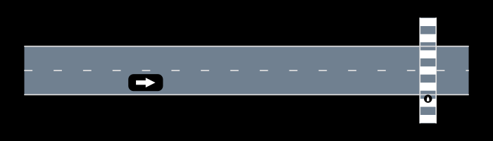
Figure 3: Layout of the autonomous vehicle scenario. A vehicle approaches a cross-walk on a neighborhood road as a single pedestrian attempts to walk across.

A-C Aircraft Collision Avoidance Software

An example result from Lee et al. [7] is shown in Figure 4. The planes need to cross paths, and the validation method was able to find a rollout where pilot responses to the ACASX system lead to an NMAC. AST was used to find a variety of different failures in ACASX.

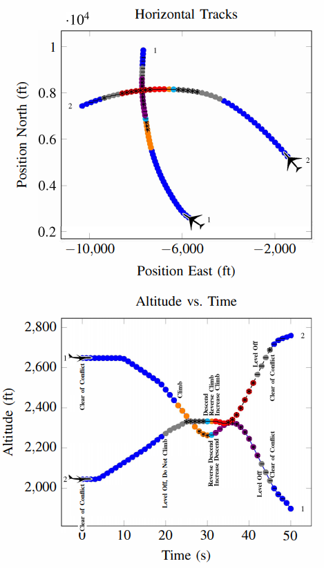
Figure 4: An example result from Lee et al. [7], showing an NMAC identified by AST. Note that the planes must be both vertically and horizontally near to each other to register as an NMAC.

References

- Barto et al. [1983] Andrew G Barto, Richard S Sutton, and Charles W Anderson. Neuronlike adaptive elements that can solve difficult learning control problems. IEEE Transactions on Systems, Man, and Cybernetics, (5):834–846, 1983.
- Kochenderfer [2015] Mykel J Kochenderfer. Decision Making Under Uncertainty. MIT Press, 2015.
- Kochenderfer et al. [2012] Mykel J Kochenderfer, Jessica E Holland, and James P Chryssanthacopoulos. Next-generation airborne collision avoidance system. Technical report, Massachusetts Institute of Technology-Lincoln Laboratory Lexington United States, 2012.
- Kocsis and Szepesvári [2006] Levente Kocsis and Csaba Szepesvári. Bandit based Monte Carlo planning. In European Conference on Machine Learning (ECML), 2006.
- Koren et al. [2018] Mark Koren, Saud Alsaif, Ritchie Lee, and Mykel J Kochenderfer. Adaptive stress testing for autonomous vehicles. In IEEE Intelligent Vehicles Symposium. IEEE, 2018.
- Kuchar and Drumm [2007] JE Kuchar and Ann C Drumm. The traffic alert and collision avoidance system. Lincoln Laboratory Journal, 16(2):277, 2007.
- Lee et al. [2015] Ritchie Lee, Mykel J Kochenderfer, Ole J Mengshoel, Guillaume P Brat, and Michael P Owen. Adaptive stress testing of airborne collision avoidance systems. In Digital Avionics Systems Conference (DASC), 2015.
- Ma et al. [2019] Xiaobai Ma, Mark Koren, Anthony Corso, Katie Driggs-Campbell, and Mykel Kochenderfer. AST toolbox: an adaptive stress testing framework for validation of autonomous systems. In IEEE/RSJ International Conference on Intelligent Robots and Systems (IROS), 2019. Submitted for review.
- Mahalanobis [1936] Prasanta Chandra Mahalanobis. On the generalised distance in statistics. Proceedings of the National Institute of Sciences of India, 2(1):49–55, 1936.
- Schulman et al. [2015] John Schulman, Sergey Levine, Pieter Abbeel, Michael Jordan, and Philipp Moritz. Trust region policy optimization. In International Conference on Machine Learning (ICML), 2015.
- Treiber et al. [2000] Martin Treiber, Ansgar Hennecke, and Dirk Helbing. Congested traffic states in empirical observations and microscopic simulations. Physics Review E, 62:1805–1824, Aug 2000.