Adaptive Stress Testing without Domain Heuristics using Go-Explore
Abstract
Recently, reinforcement learning (RL) has been used as a tool for finding failures in autonomous systems. During execution, the RL agents often rely on some domain-specific heuristic reward to guide them towards finding failures, but constructing such a heuristic may be difficult or infeasible. Without a heuristic, the agent may only receive rewards at the time of failure, or even rewards that guide it away from failures. For example, some approaches give rewards for taking more likely actions, in order to to find more likely failures. However, the agent may then learn to only take likely actions, and may not be able to find a failure at all. Consequently, the problem becomes a hard-exploration problem, where rewards do not aid exploration. A new algorithm, go-explore (GE), has recently set new records on benchmarks from the hard-exploration field. We apply GE to adaptive stress testing (AST), one example of an RL-based falsification approach that provides a way to search for the most likely failure scenario. We simulate a scenario where an autonomous vehicle drives while a pedestrian is crossing the road. We demonstrate that GE is able to find failures without domain-specific heuristics, such as the distance between the car and the pedestrian, on scenarios that other RL techniques are unable to solve. Furthermore, inspired by the robustification phase of GE, we demonstrate that the backwards algorithm (BA) improves the failures found by other RL techniques.
I Introduction
Safety validation remains a challenge in the development of autonomous vehicles [1, 2]. A promising approach is to treat validation as a reinforcement learning (RL) falsification task, in which the goal is to find scenarios that lead to a system failure using RL. For example, Akazaki et al. apply deep reinforcement learning (DRL) methods to perform falsification of signal temporal logic properties of cyber-physical systems [3]. Zhang et al. use Monte Carlo tree search (MCTS) in conjunction with hill-climbing to perform optimization-based falsification on hybrid systems [3]. Delmas et al. use MCTS for property falsification on hybrid flight controllers [4]. Adaptive stress testing (AST) [5], an RL-based method for finding the most likely failure, and is the falsification approach used in this paper.
In AST, we treat both the system under test and the simulation as a black-box environment that is controlled by actions from the AST solver, which acts as the agent in our Markov decision process (MDP) [6]. Therefore, falsification becomes a sequential decision making problem, which reinforcement learning is well-suited to solve. The formulation provides two distinct advantages: 1) we can use RL to efficiently search the space of possible actions for failures and 2) we receive an approximation of the most likely error, which allows designers to characterize how their system is most vulnerable to failure. The process is shown in fig. 1, where the AST solver takes actions and then receives rewards from the simulation. The reward can be conceptually decomposed into two parts: 1) A large penalty applied when the trajectory does not end in failure and 2) a cost at each timestep proportional to the negative log-likelihood of actions taken, such that more likely actions are penalized less. The scale of the rewards is such that the AST agent should prioritize unlikely failures over likely non-failures, but also prefer more likely failures to less likely failures. Consequently, maximizing reward leads to the most likely failure.
A difficulty arises from the fact that the failure-finding cost is only applied at the end of trajectories. Even worse, the likelihood component applied at each timestep does not actually inform the AST agent on how to find a failure. A mature system would only fail for a series of unlikely actions, so the per-step reward may actually be leading the agent away from failures. One approach is to add a heuristic reward (for example, the miss distance between a pedestrian and a car) to guide the agent towards failures [6], but creating a heuristic may be difficult or infeasible.
In reinforcement learning, a problem where reward signals are rare is known as a sparse rewards problem or a hard-exploration problem [7]. Solving hard-exploration problems is an active subset of RL research, with one of the most famous canonical baselines being the Atari game Montezuma’s Revenge [8, 9, 10]. Montezuma’s Revenge requires completing multiple sub-tasks that do not give reward in order to advance to the next level, and the horizon is sufficiently long such that the agent may never randomly discover the right sequence. Recently, the newly released go-explore (GE) algorithm was able to set new records on Montezuma’s Revenge [11].
The go-explore algorithm has two phases. Phase 1 consists of a biased random tree search that has shown state-of-the-art performance on hard-exploration problems with long horizons, like Montezuma’s Revenge. While validation tasks may not have trajectories nearly as long as Montezuma’s Revenge, having horizons of tens or even hundreds of steps is possible, especially when working with high-fidelity simulators. Phase 2 consists of “robustifying” the results by training a neural network policy using the output of phase 1 as an expert demonstration. While a falsification trajectory does not need to be robust to noise in a traditional sense, phase 2 does allow us to use the strengths of deep learning to improve our results from phase 1 while giving us more coverage of a scenario.
One of the advantages of the AST approach is that independent advancements in RL, a much larger field of research, can be applied to the solvers to improve the validation of autonomous systems [12, 13]. We demonstrate that principle by modifying GE to work on an autonomous vehicle validation task, and comparing it to the results of two previous RL solvers that we have presented: 1) a Monte Carlo tree search (MCTS) solver, and 2) a deep reinforcement learning (DRL) solver. This paper contributes the following:
-
•
We present a modification of GE better suited for general validation tasks.
-
•
We demonstrate that using GE allows us to find failures on hard-exploration scenarios for which MCTS and DRL could not find failures.
-
•
We demonstrate that applying the robustification phase to our previous solvers allows us to improve our validation results on scenarios that do not involve hard-exploration.
These contributions advance the ability of AST to find failures as well as to maximize their likelihood.
This work is organized as follows. Section II outlines the concepts of AST and RL. Section III explains the modifications made to GE for validation. Section IV provides the implementation details of our experiment. Section V demonstrates GE on longer-horizon validation tasks and shows the benefits of a robustification phase.
II Adaptive Stress Testing
II-A Markov Decision Process
AST frames the problem of finding a failure in simulation as a Markov decision process (MDP). At each timestep, an agent takes action from state . The agent may receive a reward based on the reward function [14]. The agent then transitions to the next state based on the transition function . The reward and transition depend only on the current state-action pair , not the history of previous actions or states, an independence assumption known as the Markov assumption. Neither the reward nor transition functions need to be deterministic.
Agents behave according to a policy , which specifies which action to take from each state. A policy can be stochastic or deterministic. The optimal policy is one that maximizes the value function, which can be found for a policy recursively:
| (1) |
where is the discount factor that controls the weight of future rewards. For smaller MDPs, the value function can be solved exactly. Larger MDPs may be solved approximately using reinforcement learning techniques.
II-B Formulation
The motivational problem for AST is finding the most likely trajectory that ends in a target set:
| (2) | ||||||
| subject to |
where is the probability of a trajectory in simulator and where, by the Markov assumption, is only a function of and . The set is generally defined to contain failure events. For example, for an autonomous vehicle might include collision states and near-misses.
We use reinforcement learning (RL) to approximately solve eq. 2. A trajectory that maximizes eq. 2 also maximizes where
| (3) |
and is the horizon [15].
AST solvers can treat the simulation and system under test as black-box components, however the following access functions must be provided by the simulator:
-
•
Initialize: Resets to a given initial state .
-
•
Step: Steps the simulation in time by drawing the next state after taking action . The function returns the probability of the action taken and an indicator whether is in or not.
-
•
IsTerminal: Returns true if the current state of the simulation is in , or if the horizon of the simulation has been reached.
We have previously presented a DRL solver as well as an MCTS solver [6]. In this paper, we also present a solver based on the go-explore algorithm.
II-C Deep Reinforcement Learning
In deep reinforcement learning (DRL), a policy is represented by a neural network parameterized by [16]. While a feed-forward neural network maps an input to an output, we use a recurrent neural network (RNN), which maps an input and a hidden state from the previous timestep to an output and an updated hidden state. An RNN is naturally suited to sequential data due to the hidden state, which is a learned latent representation of the current state. RNNs suffer from exploding or vanishing gradients, a problem addressed by variations such as long-short term memory (LSTM) [17] or gated recurrent unit (GRU) [18] networks.
There are many different algorithms for optimizing a neural network, but proximal policy optimization (PPO) [19] is one of the most popular. PPO is a policy-gradient method that updates the network parameters to minimize the cost function. Improvement in a policy, compared to the old policy, is measured by an advantage function. There are a variety of ways to estimate an advantage function, such as generalized advantage estimation (GAE) [20], which allows optimization over batches of trajectories. However, variance in the advantage estimate can lead to poor performance if the policy changes too much in a single step. To prevent this, PPO can limit the step size in two ways: 1) by incorporating a penalty proportional to the KL-divergence between the new and old policy or 2) by clipping the estimated advantage function when the new and old policies are too different.
II-D Monte Carlo Tree Search
Monte Carlo tree search (MCTS) [21] is one of the best-known planning algorithms, and has a long history of performing well on large MDPs [22]. MCTS is an anytime online sampling-based method that builds a tree where the nodes represent states and actions. While executing from states in the tree, MCTS chooses the action that maximizes
| (4) |
where is the expected return associated with a state-action pair, and are the number of times a state and a state-action pair have been visited, respectively, and is a parameter that controls exploration. The value is updated by executing rollouts to a specified depth and then returning the reward, which is then back-propagated up the tree. This paper uses a variation of MCTS with double progressive widening (DPW) [23] to limit the branching of the tree, which can improve performance on problems with large or continuous action spaces.
II-E Go-Explore
The go-explore (GE) algorithm is designed for hard-exploration problems [11]. The algorithm consists of an exploration-until-solved phase and a robustification phase.
II-E1 Phase 1 —Explore until solved
Phase 1 is essentially a biased random tree search that takes advantage of determinism for exploration. During phase 1, a pool of “cells” is maintained, where a cell is a data-structure indexed by a compressed mapping of the agent’s state. During rollouts, any “unseen” cell is added to the pool. If a cell has already been seen before, we compare the old version and the newly visited version. If the new cell has a better score, or has a shorter trajectory before being reached, then we replace the old cell with the new cell. Every rollout starts by randomly sampling a cell from the cell pool, which serves as the starting condition. Fundamentally, the agent deterministically follows the same trajectory back to the sampled cell, and then explores from there. The authors present multiple strategies for sampling cells from the cell pool to achieve better results. The exploration process continues for a set number of iterations or until a solution is found.
II-E2 Phase 2 —Robustification
Phase 2 uses the best result from phase 1 to train a robust policy. The result from phase 1 serves as our expert demonstration in an imitation learning task, also known as learning from demonstration (LfD). While other imitation learning algorithms could be used, the authors use the backwards algorithm (BA) [24], because of its potential to improve upon the expert demonstration. Under BA, a policy first starts training by executing rollouts from the last step of the expert trajectory. Any standard deep-learning optimization technique, such as PPO, can be used for training. The policy trains from this step of the trajectory until it does as well or better than the expert’s score. Then the starting point of training rollouts is moved one step back in the expert trajectory, to the second-to-last step, and training repeats. The process continues training and moving the starting point back until the agent is able to do as well or better than the expert on rollouts from the start of the expert trajectory. The deep-learning agent is able to efficiently learn to overcome stochastic deviations from the expert trajectory, and may discover and exploit even better strategies, if the expert trajectory is not optimal.
III Methodology
This paper applies GE to a validation task without the use of a domain-specific heuristic reward. We show that phase 1 of the algorithm is able to find failures without the use of heuristics on problem instantiations that other solvers fail on. Furthermore, we are able to use phase 2 of the algorithm to improve the results of all RL solvers that we have previously published. This section explains our modifications to both phases of the algorithm to apply GE to falsification.
III-A Phase 1
In GE, a cell is indexed by a compressed representation of the simulator state, which is also used to deterministically reset the simulation to a specific cell. AST is designed to be able to treat the simulator as a black-box (although benefits can be obtained if white-box simulation information is available). To preserve the black-box assumption, we index cells by hashing a concatenation of the current step number with the discretized action , so the index is . Therefore, similar actions at the same step of the simulation will be treated as the same cell, preserving the black-box assumption by eliminating the dependence on simulation state. Furthermore, by tracking the history of actions taken to arrive at each cell, we are able to deterministically reset to a cell without the simulation state. Instead, the agent deterministically repeats the actions in the cell’s history.
A key component of phase 1 of GE is the cell selection heuristic. Cells are assigned a fitness score, which is then normalized across all cells. Every rollout starts from a cell selected at random from the pool with probability equal to the normalized fitness score of each cell. The fitness score is partially made up of “count subscores” for three attributes that represent how often a cell has been interacted with: 1) the number of times a cell has been chosen to start a rollout, 2) the number of times a cell has been visited, and 3) the number of times a cell has been chosen since a rollout from that cell has resulted in the discovery of a new or improved cell. For each of these three attributes, a count subscore for cell and attribute can be calculated as,
| (5) |
where is the value of attribute for cell , and , , , and are hyperparameters. The total unnormalized fitness score is then
| (6) |
When applied to Montezuma’s Revenge, the authors used a ScoreWeight based on what level a cell had reached, which favored cells that had progressed furthest within the game. Progressing furthest does not have a direct analog to our validation task, so we present our own ScoreWeight. Similar to MCTS, cells track an estimate of the value function. Anytime a new cell is added to the pool or a cell is updated, the value estimate for a specific cell is updated as,
| (7) |
where is the cell’s reward, is the number of times we have seen the cell, and is the maximum value estimate of cells that are immediate children of the current cell. When a cell is updated, it then propagates the update to its parent, and so forth up the tree. The total unnormalized fitness score is calculated with . Cells with high value estimates are selected more often.
III-B Phase 2
Phase 2 of GE was designed to create a policy robust to stochastic noise, while potentially improving upon the expert demonstration. Within the context of AST, however, phase 2 acts as a hill-climbing step. AST is designed to find the most likely failure even in high-dimensional state and action spaces. However, large action-spaces can make it difficult to converge reliably to a consistent result, due to lack of coverage of the action space. While phase 1 can provide a good guess for the most likely failure trajectory, phase 2 allows us to approximately search the space of similar trajectories to find the best one. This idea is applicable to all of the solvers we have used on AST so far, and we demonstrate this by using it to improve every failure trajectory found in this paper. Phase 2 is most useful for the tree-search methods in particular (MCTS and GE), as they typically demonstrate better exploration in harder scenarios, but at the expense of converging to high-reward trajectories.
In the GE paper, as well as the original BA paper, a policy was trained from a specific step of the expert trajectory until it learned to do as well, or better. In the validation tasks we are interested in, compute may be too limited to be able to train for indefinite amounts of time. Instead, we modify BA to instead train for a small number of epochs at each step of the expert trajectory. This modification allows the number of total iterations to be specified and known ahead of time, and does not prevent phase 2 from improving the expert trajectory in any of our experiments.
IV Experiment
IV-A Problem Description
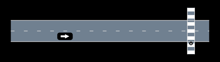
The validation scenario consists of a vehicle approaching a crosswalk on a neighborhood road as a pedestrian is trying to cross, as shown in fig. 2. The car is approaching at the speed limit of (). The vehicle, a modified version [6] of the intelligent driver model (IDM) [25], has noisy observations of the position and velocity of the pedestrian. The AST solver controls the simulation through a six-dimensional action space, consisting of the and components for three parameters: 1) the pedestrian acceleration, 2) the noise on the pedestrian position, and 3) the noise on the pedestrian velocity. We treat the simulation as a black-box, so the AST agent only has access to the initial conditions and the history of previous actions. From this general set-up, we instantiate three specific scenarios, which are differentiated by the difficulty of finding a failure. The settings changed between the scenarios include whether a reward heuristic was used (see section IV-B), the initial location of the pedestrian, as well as the rollout horizon and timestep size. Pedestrian and vehicle location are measured from the origin, which is located at the intersection of the center of the crosswalk and the center of the vehicle’s lane. The scenario parameters are shown in table I. The easy scenario is designed such that the average action leads to a collision, so the maximum possible reward is known to be . The medium and hard scenarios require unlikely actions to be taken to force a collision. They have the same initial conditions, except the hard scenario has a timestep half the duration of the medium scenario, and therefore double the maximum path length. The hard scenario demonstrates the effect of horizon length on exploration difficulty.
| Variable | Easy | Medium | Hard |
|---|---|---|---|
| steps | steps | steps | |
IV-B Modified Reward Function
We make some modifications to the theoretical reward function shown in eq. 3 to allow practical implementation:
| (8) |
where is the Mahalanobis distance [26] between the action and the expected action given the covariance matrix in the current state and is the distance between the pedestrian and the vehicle at the end of the rollout. The latter reward is the domain-specific heuristic reward that guides AST solvers by giving less penalty when the scenario ends with a pedestrian closer to the car. We use and for the easy scenario, and for the medium and hard scenarios, to disable the heuristic.
IV-C Solvers
For each experiment, the DRL, MCTS, and GE solvers were run for iterations each with a batch size of . For each solver that finds a failure, BA was then run for iterations with a batch size of , with the results reported as DRL+BA, MCTS+BA, and GE+BA, respectively.
IV-C1 Go-Explore Phase 1
GE was run with hyperparameters similar to those used for Montezuma’s Revenge. For the count subscore attributes (times chosen, times chosen since improvement, and times seen), we set equal to , , and respectively. All attributes share , , and . We always use a discount factor of . During rollouts, actions are sampled uniformly.
IV-C2 Deep Reinforcement Learning
The DRL solver uses a Gaussian-LSTM trained with PPO and GAE. The LSTM has a hidden layer size of units, and uses peephole connections [27]. For PPO, we used both a KL penalty with factor as well as a clipping range of . GAE uses a discount of and . There is no entropy coefficient.
IV-C3 Monte Carlo Tree Search
We use MCTS with DPW where rollout actions are sampled uniformly from the action space. The exploration constant was . The DPW parameters are set to and .
IV-C4 Backwards Algorithm
BA represents the policy with a Gaussian-LSTM, and optimizes the policy with PPO and GAE. The hyperparameters are identical to the DRL solver.
V Results
The results of all three solvers on the easy scenario are shown in fig. 3. All three algorithms are able to find failures quickly when given access to a heursitic reward. GE performs the worst, and both GE and MCTS show little improvement after finding their first failure. The DRL solver, however, continues to improve over the 100 iterations, ending with the best reward, and therefore the likeliest failure. This scenario is contrived such that the likeliest actions lead to collision, and even the DRL solver still was not near the optimal reward of 0. In contrast, adding robustification through BA resulted in significantly closer to optimal behavior. While GE significantly improved with robustification, GE+BA was still outperformed by DRL. However, both MCTS+BA and DRL+BA were able converge to results very near to 0.
Figure 4 shows the results of the non-DRL solvers on the medium difficulty scenario. Without a heuristic to provide reward signal, the DRL solver was unable to find a failure within 100 iterations. With the short horizon, MCTS is still able to outperform GE. Adding a robustification phase again improves both algorithms, and again the MCTS+BA solver outperforms the GE+BA solver. Note that taking the average action is not sufficient to cause a crash in this scenario.
Figure 5 shows the results of GE and GE+BA on the hard difficulty scenario. The hard scenario has a longer horizon, which prevented both DRL and MCTS from being able to find failures within 100 iterations. GE was still able to find failures, and GE+BA was still able to improve the results. In fact, when adjusting for the increased number of steps, the GE and GE+BA results on the hard scenario are very similar to those on the medium scenario, showing that GE is robust in longer horizon problems.
The results across the three scenarios illuminate the strengths and weaknesses of the three algorithms. When a useful reward signal is present, the DRL solver shows the best ability to find the most likely failure. However, without a heuristic, it quickly loses its ability to find failures. In a no-heuristic setting, MCTS is able to find more likely failures than GE as long as the problem’s horizon is short. However, in longer horizon problems GE is able to find failures that MCTS cannot The underlying principle of these differences is how the algorithms balance exploration and exploitation, which also explains why adding a robustification phase is consistently able to improve results across all three algorithms. The robustification phase applies the strength of DRL, exploitation, to a domain that requires significantly less exploration. Consequently, these two-phase methods could also be seen as an exploration phase and an exploitation phase, a problem decomposition that is easier to solve.
VI Conclusion
This paper presented an approach for validating autonomous vehicles without the use of heuristic rewards. Without a heuristic reward, the RL agent does not have a reward signal guiding it towards its goal, a type of problem known as hard-exploration . We used a modified version of go-explore, a state-of-the-art algorithm for hard-exploration. GE was able to find failures on longer horizon problems where MCTS and DRL could not. Furthermore, inspired by the robustification phase of GE, we were able to use the backwards algorithm to improve the results of all three solvers. Future work can focus further on decomposing validation into an exploration phase and an exploitation phase to take advantage of the strengths of different solvers.
References
- [1] P. Koopman, “The heavy tail safety ceiling,” in Automated and Connected Vehicle Systems Testing Symposium, 2018.
- [2] N. Kalra and S. M. Paddock, “Driving to safety: How many miles of driving would it take to demonstrate autonomous vehicle reliability?” Transportation Research Part A: Policy and Practice, vol. 94, pp. 182–193, 2016.
- [3] T. Akazaki, S. Liu, Y. Yamagata, Y. Duan, and J. Hao, “Falsification of cyber-physical systems using deep reinforcement learning,” in International Symposium on Formal Methods. Springer, 2018, pp. 456–465.
- [4] R. Delmas, T. Loquen, J. Boada-Bauxell, and M. Carton, “An evaluation of Monte-Carlo tree search for property falsification on hybrid flight control laws,” in International Workshop on Numerical Software Verification. Springer, 2019, pp. 45–59.
- [5] R. Lee, M. J. Kochenderfer, O. J. Mengshoel, G. P. Brat, and M. P. Owen, “Adaptive stress testing of airborne collision avoidance systems,” in Digital Avionics Systems Conference (DASC), 2015.
- [6] M. Koren, S. Alsaif, R. Lee, and M. J. Kochenderfer, “Adaptive stress testing for autonomous vehicles,” in IEEE Intelligent Vehicles Symposium, 2018.
- [7] M. Bellemare, S. Srinivasan, G. Ostrovski, T. Schaul, D. Saxton, and R. Munos, “Unifying count-based exploration and intrinsic motivation,” in Advances in Neural Information Processing Systems (NeurIPS), 2016, pp. 1471–1479.
- [8] Y. Burda, H. Edwards, A. Storkey, and O. Klimov, “Exploration by random network distillation,” arXiv preprint arXiv:1810.12894, 2018.
- [9] V. Mnih, K. Kavukcuoglu, D. Silver, A. A. Rusu, J. Veness, M. G. Bellemare, A. Graves, M. Riedmiller, A. K. Fidjeland, G. Ostrovski, et al., “Human-level control through deep reinforcement learning,” Nature, vol. 518, no. 7540, pp. 529–533, 2015.
- [10] N. Lipovetzky, M. Ramirez, and H. Geffner, “Classical planning with simulators: Results on the atari video games,” in International Joint Conference on Artificial Intelligence (IJCAI), 2015.
- [11] A. Ecoffet, J. Huizinga, J. Lehman, K. O. Stanley, and J. Clune, “Go-explore: a new approach for hard-exploration problems,” arXiv preprint arXiv:1901.10995, 2019.
- [12] M. Koren and M. J. Kochenderfer, “Efficient autonomy validation in simulation with adaptive stress testing,” in IEEE International Conference on Intelligent Transportation Systems (ITSC), 2019, pp. 4178–4183.
- [13] A. Corso, P. Du, K. Driggs-Campbell, and M. J. Kochenderfer, “Adaptive stress testing with reward augmentation for autonomous vehicle validation,” in IEEE International Conference on Intelligent Transportation Systems (ITSC), 2019, pp. 163–168.
- [14] M. J. Kochenderfer, Decision Making Under Uncertainty. MIT Press, 2015.
- [15] M. Koren, A. Corso, and M. Kochenderfer, “The adaptive stress testing formulation,” Robotics: Science and Systems, 2019.
- [16] I. Goodfellow, Y. Bengio, and A. Courville, Deep learning. MIT press, 2016.
- [17] S. Hochreiter and J. Schmidhuber, “Long short-term memory,” Neural Computation, vol. 9, no. 8, pp. 1735–1780, 1997.
- [18] D. Bahdanau, K. Cho, and Y. Bengio, “Neural machine translation by jointly learning to align and translate,” arXiv preprint arXiv:1409.0473, 2014.
- [19] J. Schulman, F. Wolski, P. Dhariwal, A. Radford, and O. Klimov, “Proximal policy optimization algorithms,” arXiv preprint arXiv:1707.06347, 2017.
- [20] J. Schulman, P. Moritz, S. Levine, M. Jordan, and P. Abbeel, “High-dimensional continuous control using generalized advantage estimation,” arXiv preprint arXiv:1506.02438, 2015.
- [21] L. Kocsis and C. Szepesvári, “Bandit based Monte Carlo planning,” in European Conference on Machine Learning (ECML), 2006.
- [22] C. B. Browne, E. Powley, D. Whitehouse, S. M. Lucas, P. I. Cowling, P. Rohlfshagen, S. Tavener, D. Perez, S. Samothrakis, and S. Colton, “A survey of Monte Carlo tree search methods,” IEEE Transactions on Computational Intelligence and AI in Games, vol. 4, no. 1, pp. 1–43, 2012.
- [23] A. Couëtoux, J.-B. Hoock, N. Sokolovska, O. Teytaud, and N. Bonnard, “Continuous upper confidence trees,” in Learning and Intelligent Optimization (LION). Springer, 2011, pp. 433–445.
- [24] T. Salimans and R. Chen, “Learning Montezuma’s Revenge from a single demonstration,” arXiv preprint arXiv:1812.03381, 2018.
- [25] M. Treiber, A. Hennecke, and D. Helbing, “Congested traffic states in empirical observations and microscopic simulations,” Physics Review E, vol. 62, pp. 1805–1824, Aug 2000.
- [26] P. C. Mahalanobis, “On the generalised distance in statistics,” Proceedings of the National Institute of Sciences of India, vol. 2, no. 1, pp. 49–55, 1936.
- [27] F. A. Gers and J. Schmidhuber, “Recurrent nets that time and count,” in IEEE International Joint Conference on Neural Networks, 2000, pp. 189–194.