Abstract

Using the method of massive operator matrix elements, we calculate the subleading QED initial state radiative corrections to the process $e^{+}e^{-}\rightarrow\gamma^{*}/Z^{*}$ for the first three logarithmic contributions from $O(\alpha^{3}L^{3}),O(\alpha^{3}L^{2}),O(\alpha^{3}L)$ to $O(\alpha^{5}L^{5}),O(\alpha^{5}L^{4}),O(\alpha^{5}L^{3})$ and compare their effects to the leading contribution $O(\alpha^{6}L^{6})$ and one more subleading term $O(\alpha^{6}L^{5})$. The calculation is performed in the limit of large center of mass energies squared $s\gg m_{e}^{2}$. These terms supplement the known corrections to $O(\alpha^{2})$, which were completed recently. Given the high precision at future colliders operating at very large luminosity, these corrections are important for concise theoretical predictions. The present calculation needs the calculation of one more two–loop massive operator matrix element in QED. The radiators are obtained as solutions of the associated Callen–Symanzik equations in the massive case. The radiators can be expressed in terms of harmonic polylogarithms to weight w = 6 of argument $z$ and $(1-z)$ and in Mellin $N$ space by generalized harmonic sums. Numerical results are presented on the position of the $Z$ peak and corrections to the $Z$ width, $\Gamma_{Z}$. The corrections calculated result into a final theoretical accuracy for $\delta M_{Z}$ and $\delta\Gamma_{Z}$ which is estimated to be of $O(30\leavevmode\nobreak\ \mathrm{keV})$ at an anticipated systematic accuracy at the FCC_ee of $\sim 100\leavevmode\nobreak\ \mathrm{keV}$. This precision cannot be reached, however, by including only the corrections up to $O(\alpha^{3})$.

1 Introduction

At the planned future $e^{+}e^{-}$ facilities which operate at high energy and at large luminosity, like the ILC, CLIC [1, 2, 3, 4], the FCC_ee [5], and also muon colliders [6], tests of the Standard Model are possible at unprecedented accuracy. This concerns a further detailed exploration of the $Z$ peak, beyond what was possible at LEP [7], detailed studies of Higgs boson production using $ZH$ final states, accurate scans of the top-quark threshold region, and various other precision measurements. Due to this the accuracy of the masses and widths of the heaviest particles of the Standard Model will be significantly improved.

One important ingredient to these experimental precision studies are the QED radiative corrections and in particular those due to initial state radiation (ISR). Very recently the $O(\alpha^{2})$ ISR corrections for the process $e^{+}e^{-}\rightarrow\gamma^{*}/Z^{*}$ have been completed in a direct calculation [8, 9, 10]. Here $\alpha$ denotes the fine structure constant. It has been shown that the result for all channels of a previous calculation [11] needed to be corrected in the non–logarithmic terms at $O(\alpha^{2})$. Agreement has been found with the results of Ref. [12]. Due to this it has also been proven that one may use the method of massive operator matrix elements (OMEs) for these calculations and that the Drell–Yan process factorizes for massive fermionic states.

In the present paper we take advantage of this method and extend the calculation to the first three logarithmic terms up to the order $O(\alpha^{5})$ beyond the complete $O(\alpha^{2})$ corrections and thus reach $O(\alpha^{5}L^{3})$. For comparison we also calculate the leading order contributions of $O(\alpha^{6}L^{6})$ and one more subleading term $O(\alpha^{6}L^{5})$, with $L=\ln(s/m_{e}^{2})$, $s$ denotes the center of mass energy squared of the annihilation process and $m_{e}$ is the electron mass. The universal corrections $O((\alpha L)^{k})$ are known in analytic form to order $k=5$, cf. [13, 14, 15, 16, 17, 18, 19, 20], accounting for the non–singlet and singlet contributions in the unpolarized and polarized case. The method used in Ref. [12] can be extended to higher orders in the coupling constant. For the first subleading term at $O(\alpha^{3})$, all ingredients forming the radiators in terms of Mellin transforms are known from the calculation of the anomalous dimensions in QCD [22], the Wilson coefficients of the massless Drell–Yan process [23, 24, 8] and the massive OMEs in [12]. To obtain the $O(\alpha^{3}L)$ and $O(\alpha^{3}L)$ correction we need also to calculate the massive OME $\Gamma^{(1)}_{\gamma e}$. This also applies to the higher order subleading contributions. This series could be continued straightforwardly to higher and higher order, for the first three terms at each order in the logarithmic expansion in Mellin $N$ space on the expense of longer and longer expressions.

It turns out that it is indeed the case that one has to reach at least corrections of the order $O(\alpha^{5}L^{4})$ for the ISR corrections to satisfy the ambitions goals at the FCC_ee of $\sim 100$ keV both for the $Z$ mass, $M_{Z}$, and the $Z$ width, $\Gamma_{Z}$, on the theoretical side. The method of massive operator matrix elements [12] makes this calculation possible. In the present approach the constant term of $O(\alpha^{3})$ and its higher order logarithmic extensions are still missing. They require still higher order massive OMEs and also massless Wilson coefficients in analytic form. Their size is, however, gradually smaller.

The paper is organized as follows. In Section 2 we present the structure of the QED ISR radiative corrections to the Born cross section following from the renormalization group equations (RGEs), for which we present the analytic solutions in terms of anomalous dimensions, massive OMEs and massless Wilson coefficients for all contributions calculated in the present paper. In Section 3 we calculate the massive OME $\Gamma^{(1)}_{\gamma e}$. The radiator functions in $z$ space for the $O(\alpha^{3})$ and $O(\alpha^{4})$ corrections are presented in Section 4. The radiators can be expressed in terms of harmonic polylogarithms [25], to which the Nielsen integrals and classical polylogarithms form a subset [26, 27]. In Section 5, we present numerical results on the corrections in the kinematic region around the $Z$ peak and we determine the corresponding corrections to the pole mass of the $Z$ boson and the $Z$ boson width, $\Gamma_{Z}$. Section 6 contains the conclusions. In Mellin $N$ space the radiators are given in terms of harmonic and generalized harmonic sums. If compared to the $z$ space representation they are more compact. Due to the appearance of generalized harmonic sums we derive in Appendix A the singularity structure of the radiators in the complex $N$-plane and in Appendix B we present all radiators calculated in the present paper in Mellin space.

2 The Initial State Corrections to the $e^{+}e^{-}$ Annihilation Cross Section

The initial state QED radiative corrections to $e^{+}e^{-}\rightarrow\gamma^{*}/Z^{*}$ can be calculated by applying the method of massive operator matrix elements, cf. [12]. It has been demonstrated by the recent complete calculation in [8, 9, 10] that the effective method of Ref. [12] is delivering the complete result. Particular non–logarithmic contributions with vanishing massive OME to the Drell–Yan process in the constant term $O(\alpha^{2})$ could be structurally absorbed in the relations and appear as contributions to the massless Wilson coefficients given in [12], Eqs. (40–42). It is due to this agreement, that one can now safely apply this method also for subleading logarithms to higher orders in the coupling constant by solving the associated renormalization group equations in the massive case. The method has been used in Ref. [11] before for the logarithmic enhanced contributions to $O(\alpha^{2}L)$.

The massive effects due to the finite electron mass $m_{e}$ enter here through process–independent massive operator matrix elements. The Wilson coefficients are those of the massless Drell–Yan process [23, 24, 8]. Note that there are differences between the corrections to the vector and axial–vector coupling.

In $z$–space the different contributions to the radiators are connected by Mellin convolutions $\otimes$ which are defined by

$$[A\otimes B](z)=\int_{0}^{1}dx_{1}\int_{0}^{1}dx_{2}\delta(1-x_{1}x_{2})A(x_{1})B(x_{2}).$$ (1)

The Mellin transform reads

$${\rm\bf M}[f(z)](N)=\int_{0}^{1}dzz^{N-1}f(z),\leavevmode\nobreak\ \leavevmode\nobreak\ \leavevmode\nobreak\ \leavevmode\nobreak\ {\rm\bf M}[[f(z)]_{+}](N)=\int_{0}^{1}dz(z^{N-1}-1)f(z)$$ (2)

for regular functions and +-distributions, respectively. The most recently calculated quantities are the massive OMEs given in [12].

The radiative corrections to the differential scattering cross section is given by

$$\frac{d\sigma_{e^{+}e^{-}}}{ds^{\prime}}=\frac{1}{s}\sigma^{(0)}\left\{1+\sum_{k=1}^{\infty}a_{0}^{k}\sum_{l=0}^{k}c_{k,l}{\rm\bf L}^{k-l}\right\}$$ (3)

in $z$ space. Here we defined

$${\rm\bf L}=L+\ln(z),\leavevmode\nobreak\ \leavevmode\nobreak\ \leavevmode\nobreak\ \leavevmode\nobreak\ \leavevmode\nobreak\ L=\ln\left(\frac{s}{m_{e}^{2}}\right),$$ (4)

and $\sigma^{(0)}$ denotes the Born cross section, cf. [12], Eq. (8), and Ref. [28]. $a_{0}=a(\mu^{2}=m_{e}^{2})$ is the normalized fine structure constant with $a(\mu^{2})=\alpha(\mu^{2})/(4\pi)$, which we will widely use in the following. Here it is convenient to refer to $a_{0}$ only and account also for all evolution contributions by the functions $c_{k,l}$.

For the Born cross section for $e^{+}e^{-}$ annihilation, $\sigma_{0}$, we will consider $s$-channel $e^{+}e^{-}$ annihilation into a virtual gauge boson $(\gamma,Z)$ which decays into a fermion pair $f\overline{f}$ and $e\neq f$. This process both describes lower energy $\gamma$-exchange and the $Z$-resonance.

$$\frac{d\sigma^{(0)}(s)}{d\Omega} = \frac{\alpha^{2}}{4s}N_{C,f}\sqrt{1-\frac{4m_{f}}{s}}$$ (5)

$$\times\left[\left(1+\cos^{2}\theta+\frac{4m_{f}^{2}}{s}\sin^{2}\theta\right)G_{1}(s)-\frac{8m_{f}^{2}}{s}G_{2}(s)+2\sqrt{1-\frac{4m_{f}^{2}}{s}}\cos\theta G_{3}(s)\right]$$

$$\times{\cal G}(s)\leavevmode\nobreak\ ,$$

$$\sigma^{(0)}(s) = \frac{4\pi\alpha^{2}}{3s}N_{C,f}\sqrt{1-\frac{4m_{f}}{s}}\left[\left(1+\frac{2m_{f}^{2}}{s}\right)G_{1}(s)-6\frac{m_{f}^{2}}{s}G_{2}(s)\right]{\cal G}(s)\leavevmode\nobreak\ ,$$ (6)

see e.g. [28, 29]. Here the final state fermions are considered to be no electrons, to obtain an $s$-channel Born cross section. In Eqs. (5, 6) the electron mass is neglected kinematically. $N_{C,f}$ is the number of colors of the final state fermion, with $N_{C,f}=1$ for colorless fermions, and $N_{C,f}=3$ for quarks. The function ${\cal G}(s)=1$ in the case of the pure perturbative calculation. $s$ is the cms energy, $\Omega$ is the spherical angle, $\theta$ the cms scattering angle, and the effective couplings $G_{i}(s)|_{i=1...3}$ read

$$G_{1}(s) = Q_{e}^{2}Q_{f}^{2}+2Q_{e}Q_{f}v_{e}v_{f}{\sf Re}[\chi_{Z}(s)]+(v_{e}^{2}+a_{e}^{2})(v_{f}^{2}+a_{f}^{2})|\chi_{Z}(s)|^{2},$$ (7)

$$G_{2}(s) = (v_{e}^{2}+a_{e}^{2})a_{f}^{2}|\chi_{Z}(s)|^{2},$$ (8)

$$G_{3}(s) = 2Q_{e}Q_{f}a_{e}a_{f}{\sf Re}[\chi_{Z}(s)]+4v_{e}v_{f}a_{e}a_{f}|\chi_{Z}(s)|^{2}.$$ (9)

The reduced $Z$–propagator is given by

$$\chi_{Z}(s)=\frac{s}{s-M_{Z}^{2}+iM_{Z}\Gamma_{Z}},$$ (10)

where $M_{Z}$ and $\Gamma_{Z}$ are the mass and the width of the $Z$ boson and $m_{f}$ is the mass of the final state fermion. $Q_{e,f}$ are the electromagnetic charges of the electron $(Q_{e}=-1)$ and the final state fermion, respectively, and the electro–weak couplings $v_{i}$ and $a_{i}$ read

$$v_{e} = \frac{1}{\sin\theta_{w}\cos\theta_{w}}\left[I^{3}_{w,e}-2Q_{e}\sin^{2}\theta_{w}\right],$$ (11)

$$a_{e} = \frac{1}{\sin\theta_{w}\cos\theta_{w}}I^{3}_{w,e},$$ (12)

$$v_{f} = \frac{1}{\sin\theta_{w}\cos\theta_{w}}\left[I^{3}_{w,f}-2Q_{f}\sin^{2}\theta_{w}\right],$$ (13)

$$a_{f} = \frac{1}{\sin\theta_{w}\cos\theta_{w}}I^{3}_{w,f}\leavevmode\nobreak\ ,$$ (14)

where $\theta_{w}$ is the weak mixing angle, and $I^{3}_{w,i}=\pm 1/2$ the third component of the weak isospin for up and down particles, respectively.

The inclusive $s$–channel annihilation scattering cross section $\sigma_{e^{+}e^{-}}$ is given by

$$\sigma_{e^{+}e^{-}}(s) = \int_{s_{0}}^{s}ds^{\prime}\frac{d\sigma_{e^{+}e^{-}}(s^{\prime})}{ds^{\prime}}=\int_{z_{0}}^{1}dz\sigma^{(0)}(sz)R(z,s/m_{e}^{2}),$$ (15)

with $s^{\prime}=sz$, $\sigma^{(0)}(s^{\prime})$ the Born cross section and $R(z,s/m_{e}^{2})$ the distribution–valued radiator [30] describing the initial state radiation of photons and light $e^{+}e^{-}$ pairs. The lower bound $s_{0}=sz_{0}$ is an invariant mass squared depending on the experiment, cf. [7]. In the later numerical illustrations we will choose $s_{0}=4m_{\tau}^{2}$, with $m_{\tau}$ the $\tau$ lepton mass.

The general decomposition of the scattering cross section in Mellin space is given by, cf. [11]

$$\frac{d\sigma_{e^{+}e^{-}}}{ds^{\prime}} = \frac{1}{s}\sigma^{(0)}(s^{\prime})\Biggl{[}\Gamma_{e^{+}e^{+}}\left(N,\frac{\mu^{2}}{m_{e}^{2}}\right)\tilde{\sigma}_{e^{+}e^{-}}\left(N,\frac{s^{\prime}}{\mu^{2}}\right)\Gamma_{e^{-}e^{-}}\left(N,\frac{\mu^{2}}{m_{e}^{2}}\right)$$ (16)

$$+\Gamma_{\gamma e^{+}}\left(N,\frac{\mu^{2}}{m_{e}^{2}}\right)\tilde{\sigma}_{e^{-}\gamma}\left(N,\frac{s^{\prime}}{\mu^{2}}\right)\Gamma_{e^{-}e^{-}}\left(N,\frac{\mu^{2}}{m_{e}^{2}}\right)$$

$$+\Gamma_{e^{+}e^{+}}\left(N,\frac{\mu^{2}}{m_{e}^{2}}\right)\tilde{\sigma}_{e^{+}\gamma}\left(N,\frac{s^{\prime}}{\mu^{2}}\right)\Gamma_{\gamma e^{-}}\left(N,\frac{\mu^{2}}{m_{e}^{2}}\right)$$

$$+\Gamma_{\gamma e^{+}}\left(N,\frac{\mu^{2}}{m_{e}^{2}}\right)\tilde{\sigma}_{\gamma\gamma}\left(N,\frac{s^{\prime}}{\mu^{2}}\right)\Gamma_{\gamma e^{-}}\left(N,\frac{\mu^{2}}{m_{e}^{2}}\right)\Biggr{]}.$$

The terms in the brackets $[...]$ are Mellin–convoluted. Only massive OMEs of the kind $\Gamma_{e^{\pm}e^{\pm}}$ and $\Gamma_{\gamma e^{\pm}}$ contribute because the process considered has electron–positron initial states. The last term in Eq. (16) is only contributing with $O(a^{4})$. $\mu$ denotes the factorization and renormalization scale. As we will see later, it will cancel in the scattering cross section, when performing the expansion consistently to a certain order in $a_{0}$. The massive OMEs, $\Gamma_{ij}$, and massless Wilson coefficients, $\tilde{\sigma}_{ij}$, obey the following series representations

$$\Gamma_{li}\left(N,\frac{\mu^{2}}{m_{e}^{2}}\right) = \delta_{li}+\sum_{r=1}^{\infty}a^{r}(\mu^{2})\sum_{n=0}^{r}a_{li;nr}(N)\Lambda^{n}$$ (17)

$$\tilde{\sigma}_{lk}\left(N,\frac{s^{\prime}}{\mu^{2}}\right) = \delta_{lk}+\sum_{r=1}^{\infty}a^{r}(\mu^{2})\sum_{n=0}^{r}b_{lk;nr}(N)\lambda^{n},$$ (18)

with the logarithms $\Lambda$ and $\lambda$ given by

$$\Lambda=\ln\left(\frac{\mu^{2}}{m_{e}^{2}}\right),\leavevmode\nobreak\ \leavevmode\nobreak\ \leavevmode\nobreak\ \leavevmode\nobreak\ \leavevmode\nobreak\ \leavevmode\nobreak\ \leavevmode\nobreak\ \lambda=\ln\left(\frac{s^{\prime}}{\mu^{2}}\right).$$ (19)

The massive OMEs $\Gamma_{ij}$ and massless Wilson coefficients $\tilde{\sigma}_{kl}$ fulfill the following renormalization group equations, cf. [33],

$$\left[\left(\frac{\partial}{\partial\Lambda}+\beta(a)\frac{\partial}{\partial a}\right)\delta_{kl}+\frac{1}{2}\gamma_{kl}(N,a)\right]\Gamma_{li}\left(N,a,\frac{\mu^{2}}{m_{e}^{2}}\right) = 0$$ (20)

$$\left[\left(\frac{\partial}{\partial\lambda}-\beta(a)\frac{\partial}{\partial a}\right)\delta_{kl}\delta_{jm}+\frac{1}{2}\gamma_{kl}(N,a)\delta_{jm}+\frac{1}{2}\gamma_{jm}(N,a)\delta_{kl}\right]\tilde{\sigma}_{lj}\left(N,a,\frac{s^{\prime}}{\mu^{2}}\right) = 0\leavevmode\nobreak\ ,$$ (21)

and the QED $\beta$ function has the representation

$$\beta(a)=-\sum_{k=0}^{\infty}\beta_{k}a^{k+2}.$$ (22)

Eq. (23) gives an overview on the orders of the expansion of the radiators in the fine structure constant which are now available, including the results of the present calculation,

$$\begin{array}[]{lll}\alpha\ {L}&\alpha&\\ \alpha^{2}{L}^{2}&\alpha^{2}{L}&\alpha^{2}\\ \alpha^{3}{L}^{3}&\alpha^{3}{L}^{2}&\alpha^{3}{L}\\ \alpha^{4}{L}^{4}&\alpha^{4}{L}^{3}&\alpha^{4}{L}^{2}\\ \alpha^{5}{L}^{5}&\alpha^{5}{L}^{4}&\alpha^{5}{L}^{3}\\ \alpha^{6}{L}^{6}&\alpha^{6}{L}^{5}\leavevmode\nobreak\ .&\end{array}$$ (23)

The expansion coefficients $c_{k,l}$ of Eq. (3) up to the sixth order in $a_{0}$ in Mellin space are given by Eqs. (25–41). They are expressed by the anomalous dimensions $\gamma_{ij}^{(k)}$ [22], the expansion coefficients of the massless Drell–Yan cross section [23, 24, 8], $\tilde{\sigma}_{ij}^{(k)}$, the expansion coefficients of the QED $\beta$ function and the renormalized massive OMEs $\Gamma_{ij}^{(k)}$, where $(k+1)$ denotes the loop order. In the following we use the notation

$$\gamma_{ij}^{(k)}=-P_{ij}^{(k)}(N)=-{\rm\bf M}[P_{ij}^{(k)}(z)](N).$$ (24)

When working in $z$ space we will use $P_{ij}^{(k)}(z)$ instead of the anomalous dimensions $\gamma_{ij}^{(k)}$.

One obtains

$$c_{1,1} = -\gamma_{ee}^{(0)},$$ (25)

$$c_{1,0} = \tilde{\sigma}_{ee}^{(0)}+2\Gamma_{ee}^{(0)},$$ (26)

$$c_{2,2} = \frac{1}{2}{\gamma_{ee}^{(0)}}^{2}+\frac{\beta_{0}}{2}\gamma_{ee}^{(0)}+\frac{1}{4}\gamma_{e\gamma}^{(0)}\gamma_{\gamma e}^{(0)},$$ (27)

$$c_{2,1} = -\gamma_{ee}^{(1)}-\gamma_{ee}^{(0)}(\tilde{\sigma}_{ee}^{(0)}+2\Gamma_{ee}^{(0)})-\beta_{0}\tilde{\sigma}_{ee}^{(0)}-\gamma_{\gamma e}^{(0)}\tilde{\sigma}_{e\gamma}^{(0)}-\Gamma_{\gamma e}^{(0)}\gamma_{e\gamma}^{(0)},$$ (28)

$$c_{2,0} = 2\Gamma_{ee}^{(1)}+\tilde{\sigma}_{ee}^{(1)}+2\Gamma_{ee}^{(0)}\tilde{\sigma}_{ee}^{(0)}+{\Gamma_{ee}^{(0)}}^{2}+2\tilde{\sigma}_{e\gamma}^{(0)}\Gamma_{\gamma e}^{(0)},$$ (29)

$$c_{3,3} = -\frac{{\gamma_{ee}^{(0)}}^{3}}{6}-\frac{\beta_{0}{\gamma_{ee}^{(0)}}^{2}}{2}-\frac{1}{4}\beta_{0}\gamma_{e\gamma}^{(0)}\gamma_{\gamma e}^{(0)}-\frac{1}{24}\gamma_{e\gamma}^{(0)}\gamma_{\gamma e}^{(0)}\gamma_{\gamma\gamma}^{(0)}-\gamma_{ee}^{(0)}\left(\frac{\beta_{0}^{2}}{3}+\frac{5\gamma_{e\gamma}^{(0)}\gamma_{\gamma e}^{(0)}}{24}\right),$$ (30)

$$c_{3,2} = \frac{\Gamma_{ee}^{(0)}\gamma_{e\gamma}^{(0)}\gamma_{\gamma e}^{(0)}}{2}+\frac{\gamma_{e\gamma}^{(1)}\gamma_{\gamma e}^{(0)}}{4}+\frac{\gamma_{e\gamma}^{(0)}\gamma_{\gamma e}^{(1)}}{4}+\frac{\gamma_{e\gamma}^{(0)}\Gamma_{\gamma e}^{(0)}\gamma_{\gamma\gamma}^{(0)}}{4}+\beta_{0}^{2}\tilde{\sigma}_{ee}^{(0)}+\frac{\gamma_{e\gamma}^{(0)}\gamma_{\gamma e}^{(0)}\tilde{\sigma}_{ee}^{(0)}}{4}$$ (31)

$$+\frac{\gamma_{\gamma e}^{(0)}\gamma_{\gamma\gamma}^{(0)}\tilde{\sigma}_{e\gamma}^{(0)}}{4}+\beta_{0}\left(\gamma_{ee}^{(1)}+\frac{\gamma_{e\gamma}^{(0)}\Gamma_{\gamma e}^{(0)}}{2}+\frac{3\gamma_{\gamma e}^{(0)}\tilde{\sigma}_{e\gamma}^{(0)}}{2}\right)+{\gamma_{ee}^{(0)}}^{2}\left(\Gamma_{ee}^{(0)}+\frac{\tilde{\sigma}_{ee}^{(0)}}{2}\right)$$

$$+{\gamma_{ee}^{(0)}}\left[\frac{\beta_{1}}{2}+\gamma^{(1)}_{ee}+\frac{3\gamma_{e\gamma}^{(0)}\Gamma_{\gamma e}^{(0)}}{4}+\frac{3\gamma_{\gamma e}^{(0)}\tilde{\sigma}_{e\gamma}^{(0)}}{4}+\beta_{0}\left(\Gamma_{ee}^{(0)}+\frac{3\tilde{\sigma}_{ee}^{(0)}}{2}\right)\right],$$

$$c_{3,1} = -\gamma_{ee}^{(2)}-2\Gamma_{ee}^{(0)}\gamma_{ee}^{(1)}-\Gamma_{ee}^{(0)}\gamma_{e\gamma}^{(0)}\Gamma_{\gamma e}^{(0)}-\gamma_{e\gamma}^{(1)}\Gamma_{\gamma e}^{(0)}-\gamma_{e\gamma}^{(0)}\Gamma_{\gamma e}^{(1)}-\beta_{1}\tilde{\sigma}_{ee}^{(0)}-\gamma_{ee}^{(1)}\tilde{\sigma}_{ee}^{(0)}$$ (32)

$$-\gamma_{e\gamma}^{(0)}\Gamma_{\gamma e}^{(0)}\tilde{\sigma}_{ee}^{(0)}-2\Gamma_{ee}^{(0)}\gamma_{\gamma e}^{(0)}\tilde{\sigma}_{e\gamma}^{(0)}-\gamma_{\gamma e}^{(1)}\tilde{\sigma}_{e\gamma}^{(0)}-\Gamma_{\gamma e}^{(0)}\gamma_{\gamma\gamma}^{(0)}\tilde{\sigma}_{e\gamma}^{(0)}-\gamma_{\gamma e}^{(0)}\tilde{\sigma}_{\gamma e}^{(1)}+\beta_{0}\Bigl{[}-2\Gamma_{ee}^{(0)}\tilde{\sigma}_{ee}^{(0)}$$

$$-2\tilde{\sigma}_{ee}^{(1)}-2\Gamma_{\gamma e}^{(0)}\tilde{\sigma}_{e\gamma}^{(0)}\Bigr{]}-\gamma_{ee}^{(0)}\left[{\Gamma_{ee}^{(0)}}^{2}+2\Gamma_{ee}^{(1)}+2\Gamma_{ee}^{(0)}\tilde{\sigma}_{ee}^{(0)}+\tilde{\sigma}_{ee}^{(1)}+\Gamma_{\gamma e}^{(0)}\tilde{\sigma}_{e\gamma}^{(0)}\right],$$

$$c_{3,0} = 2\Gamma_{ee}^{(2)}+\tilde{\sigma}_{ee}^{(2)}+2\Gamma_{ee}^{(0)}\Gamma_{ee}^{(1)}+\left[{\Gamma_{ee}^{(0)}}^{2}+2\Gamma_{ee}^{(1)}\right]\tilde{\sigma}_{ee}^{(0)}+2\Gamma_{ee}^{(0)}\tilde{\sigma}_{ee}^{(1)}+2\left[\Gamma_{ee}^{(0)}\Gamma_{\gamma e}^{(0)}+\Gamma_{\gamma e}^{(1)}\right]\tilde{\sigma}_{e\gamma}^{(0)}$$ (33)

$$+2\Gamma_{\gamma e}^{(0)}\tilde{\sigma}_{\gamma e}^{(1)}$$

$$c_{4,4} = \frac{{\gamma_{ee}^{(0)}}^{4}}{24}+\frac{\beta_{0}}{4}{\gamma_{ee}^{(0)}}^{3}+\frac{11}{48}\beta_{0}^{2}\gamma_{e\gamma}^{(0)}\gamma_{\gamma e}^{(0)}+\left[11\beta_{0}^{2}+\frac{17}{8}\gamma_{e\gamma}^{(0)}\gamma_{\gamma e}^{(0)}\right]\frac{{\gamma_{ee}^{(0)}}^{2}}{24}+\biggl{[}\beta_{0}^{3}+\frac{5}{4}\beta_{0}\gamma_{e\gamma}^{(0)}\gamma_{\gamma e}^{(0)}$$ (34)

$$+\frac{1}{8}\gamma_{\gamma\gamma}^{(0)}\gamma_{e\gamma}^{(0)}\gamma_{\gamma e}^{(0)}\biggr{]}\frac{\gamma_{ee}^{(0)}}{4}+\frac{1}{16}\beta_{0}\gamma_{\gamma\gamma}^{(0)}\gamma_{e\gamma}^{(0)}\gamma_{\gamma e}^{(0)}+\frac{1}{192}\gamma_{e\gamma}^{(0)}\gamma_{\gamma e}^{(0)}\left[4\gamma_{e\gamma}^{(0)}\gamma_{\gamma e}^{(0)}+{\gamma_{\gamma\gamma}^{(0)}}^{2}\right],$$

$$c_{4,3} = -\frac{5}{6}\beta_{0}\beta_{1}\gamma_{ee}^{(0)}-\frac{1}{2}\beta_{1}{\gamma_{ee}^{(0)}}^{2}-\frac{2}{3}\beta_{0}^{2}\gamma_{ee}^{(0)}\Gamma_{ee}^{(0)}-\beta_{0}{\gamma_{ee}^{(0)}}^{2}\Gamma_{ee}^{(0)}-\frac{1}{3}{\gamma_{ee}^{(0)}}^{3}\Gamma_{ee}^{(0)}-\beta_{0}^{2}\gamma_{ee}^{(1)}$$ (35)

$$-\frac{3}{2}\beta_{0}\gamma_{ee}^{(0)}\gamma_{ee}^{(1)}-\frac{1}{2}{\gamma_{ee}^{(0)}}^{2}\gamma_{ee}^{(1)}-\frac{1}{4}\beta_{1}\gamma_{e\gamma}^{(0)}\gamma_{\gamma e}^{(0)}-\frac{1}{2}\beta_{0}\Gamma_{ee}^{(0)}\gamma_{e\gamma}^{(0)}\gamma_{\gamma e}^{(0)}-\frac{5}{12}\gamma_{ee}^{(0)}\Gamma_{ee}^{(0)}\gamma_{e\gamma}^{(0)}\gamma_{\gamma e}^{(0)}$$

$$-\frac{5}{24}\gamma_{ee}^{(1)}\gamma_{e\gamma}^{(0)}\gamma_{\gamma e}^{(0)}-\frac{5}{12}\beta_{0}\gamma_{e\gamma}^{(1)}\gamma_{\gamma e}^{(0)}-\frac{5}{24}\gamma_{ee}^{(0)}\gamma_{e\gamma}^{(1)}\gamma_{\gamma e}^{(0)}-\frac{1}{3}\beta_{0}^{2}\gamma_{e\gamma}^{(0)}\Gamma_{\gamma e}^{(0)}-\frac{3}{4}\beta_{0}\gamma_{ee}^{(0)}\gamma_{e\gamma}^{(0)}\Gamma_{\gamma e}^{(0)}$$

$$-\frac{7}{24}{\gamma_{ee}^{(0)}}^{2}\gamma_{e\gamma}^{(0)}\Gamma_{\gamma e}^{(0)}-\frac{1}{6}{\gamma_{e\gamma}^{(0)}}^{2}\gamma_{\gamma e}^{(0)}\Gamma_{\gamma e}^{(0)}-\frac{1}{3}\beta_{0}\gamma_{e\gamma}^{(0)}\gamma_{\gamma e}^{(1)}-\frac{5}{24}\gamma_{ee}^{(0)}\gamma_{e\gamma}^{(0)}\gamma_{\gamma e}^{(1)}-\frac{1}{12}\Gamma_{ee}^{(0)}\gamma_{e\gamma}^{(0)}\gamma_{\gamma e}^{(0)}\gamma_{\gamma\gamma}^{(0)}$$

$$-\frac{1}{24}\gamma_{e\gamma}^{(1)}\gamma_{\gamma e}^{(0)}\gamma_{\gamma\gamma}^{(0)}-\frac{1}{4}\beta_{0}\gamma_{e\gamma}^{(0)}\Gamma_{\gamma e}^{(0)}\gamma_{\gamma\gamma}^{(0)}-\frac{1}{6}\gamma_{ee}^{(0)}\gamma_{e\gamma}^{(0)}\Gamma_{\gamma e}^{(0)}\gamma_{\gamma_{\gamma}}^{(0)}-\frac{1}{24}\gamma_{e\gamma}^{(0)}\gamma_{\gamma e}^{(1)}\gamma_{\gamma\gamma}^{(0)}-\frac{1}{24}\gamma_{e\gamma}^{(0)}\Gamma_{\gamma e}^{(0)}{\gamma_{\gamma\gamma}^{(0)}}^{2}$$

$$-\frac{1}{24}\gamma_{e\gamma}^{(0)}\gamma_{\gamma e}^{(0)}\gamma_{\gamma\gamma}^{(1)}-\beta_{0}^{3}\tilde{\sigma}_{ee}^{(0)}-\frac{11}{6}\beta_{0}^{2}\gamma_{ee}^{(0)}\tilde{\sigma}_{ee}^{(0)}-\beta_{0}{\gamma_{ee}^{(0)}}^{2}\tilde{\sigma}_{ee}^{(0)}-\frac{1}{6}{\gamma_{ee}^{(0)}}^{3}\tilde{\sigma}_{ee}^{(0)}-\frac{1}{2}\beta_{0}\gamma_{e\gamma}^{(0)}\gamma_{\gamma e}^{(0)}\tilde{\sigma}_{ee}^{(0)}$$

$$-\frac{5}{24}\gamma_{ee}^{(0)}\gamma_{e\gamma}^{(0)}\gamma_{\gamma e}^{(0)}\tilde{\sigma}_{ee}^{(0)}-\frac{1}{24}\gamma_{e\gamma}^{(0)}\gamma_{\gamma e}^{(0)}\gamma_{\gamma\gamma}^{(0)}\tilde{\sigma}_{ee}^{(0)}-\frac{11}{6}\beta_{0}^{2}\gamma_{\gamma e}^{(0)}\tilde{\sigma}_{\gamma e}^{(0)}-\frac{3}{2}\beta_{0}\gamma_{ee}^{(0)}\gamma_{\gamma_{e}}^{(0)}\tilde{\sigma}_{\gamma_{e}}^{(0)}$$

$$-\frac{7}{24}{\gamma_{ee}^{(0)}}^{2}\gamma_{\gamma e}^{(0)}\tilde{\sigma}_{\gamma e}^{(0)}-\frac{1}{6}\gamma_{e\gamma}^{(0)}{\gamma_{\gamma e}^{(0)}}^{2}\tilde{\sigma}_{\gamma_{e}}^{(0)}-\frac{1}{2}\beta_{0}\gamma_{\gamma e}^{(0)}\gamma_{\gamma\gamma}^{(0)}\tilde{\sigma}_{\gamma e}^{(0)}-\frac{1}{6}\gamma_{ee}^{(0)}\gamma_{\gamma e}^{(0)}\gamma_{\gamma\gamma}^{(0)}\tilde{\sigma}_{\gamma e}^{(0)}$$

$$-\frac{1}{24}\gamma_{\gamma e}^{(0)}{\gamma_{\gamma\gamma}^{(0)}}^{2}\tilde{\sigma}_{\gamma e}^{(0)},$$

$$c_{4,2} = \frac{1}{2}\beta_{2}\gamma_{ee}^{(0)}+\beta_{1}\gamma_{ee}^{(0)}\Gamma_{ee}^{(0)}+\frac{1}{2}\beta_{0}\gamma_{ee}^{(0)}{\Gamma_{ee}^{(0)}}^{2}+\frac{1}{2}{\gamma_{ee}^{(0)}}^{2}{\Gamma_{ee}^{(0)}}^{2}+\beta_{1}\gamma_{ee}^{(1)}$$ (36)

$$+2\beta_{0}\Gamma_{ee}^{(0)}\gamma_{ee}^{(1)}+2\gamma_{ee}^{(0)}\Gamma_{ee}^{(0)}\gamma_{ee}^{(1)}+\frac{1}{2}{\gamma_{ee}^{(1)}}^{2}+\beta_{0}\gamma_{ee}^{(0)}\Gamma_{ee}^{(1)}+{\gamma_{ee}^{(0)}}^{2}\Gamma_{ee}^{(1)}$$

$$+\frac{3}{2}\beta_{0}\gamma_{ee}^{(2)}+\gamma_{ee}^{(0)}\gamma_{ee}^{(2)}+\frac{1}{4}{\Gamma_{ee}^{(0)}}^{2}\gamma_{e\gamma}^{(0)}\gamma_{\gamma e}^{(0)}+\frac{1}{2}\Gamma_{ee}^{(1)}\gamma_{e\gamma}^{(0)}\gamma_{\gamma e}^{(0)}+\frac{1}{2}\Gamma_{ee}^{(0)}\gamma_{e\gamma}^{(1)}\gamma_{\gamma e}^{(0)}$$

$$+\frac{1}{4}\gamma_{e\gamma}^{(2)}\gamma_{\gamma e}^{(0)}+\frac{1}{2}\beta_{1}\gamma_{e\gamma}^{(0)}\Gamma_{\gamma e}^{(0)}+\frac{1}{2}\beta_{0}\Gamma_{ee}^{(0)}\gamma_{e\gamma}^{(0)}\Gamma_{\gamma e}^{(0)}+\frac{3}{4}\gamma_{ee}^{(0)}\Gamma_{ee}^{(0)}\gamma_{e\gamma}^{(0)}\Gamma_{\gamma e}^{(0)}+\frac{3}{4}\gamma_{ee}^{(1)}\gamma_{e\gamma}^{(0)}\Gamma_{\gamma e}^{(0)}$$

$$+\beta_{0}\gamma_{e\gamma}^{(1)}\Gamma_{\gamma e}^{(0)}+\frac{3}{4}\gamma_{ee}^{(0)}\gamma_{e\gamma}^{(1)}\Gamma_{\gamma e}^{(0)}+\frac{1}{4}{\gamma_{e\gamma}^{(0)}}^{2}{\Gamma_{\gamma e}^{(0)}}^{2}+\frac{1}{2}\Gamma_{ee}^{(0)}\gamma_{e\gamma}^{(0)}\gamma_{\gamma e}^{(1)}+\frac{1}{4}\gamma_{e\gamma}^{(1)}\gamma_{\gamma e}^{(1)}$$

$$+\frac{1}{2}\beta_{0}\gamma_{e\gamma}^{(0)}\Gamma_{\gamma e}^{(1)}+\frac{3}{4}\gamma_{ee}^{(0)}\gamma_{e\gamma}^{(0)}\Gamma_{\gamma e}^{(1)}+\frac{1}{4}\gamma_{e\gamma}^{(0)}\gamma_{\gamma e}^{(2)}+\frac{1}{4}\Gamma_{ee}^{(0)}\gamma_{e\gamma}^{(0)}\Gamma_{\gamma e}^{(0)}\gamma_{\gamma\gamma}^{(0)}+\frac{1}{4}\gamma_{e\gamma}^{(1)}\Gamma_{\gamma e}^{(0)}\gamma_{\gamma\gamma}^{(0)}$$

$$+\frac{1}{4}\gamma_{e\gamma}^{(0)}\Gamma_{\gamma e}^{(1)}\gamma_{\gamma\gamma}^{(0)}+\frac{1}{4}\gamma_{e\gamma}^{(0)}\Gamma_{\gamma e}^{(0)}\gamma_{\gamma\gamma}^{(1)}+\frac{5}{2}\beta_{0}\beta_{1}\tilde{\sigma}_{ee}^{(0)}+\frac{3}{2}\beta_{1}\gamma_{ee}^{(0)}\tilde{\sigma}_{ee}^{(0)}+2\beta_{0}^{2}\Gamma_{ee}^{(0)}\tilde{\sigma}_{ee}^{(0)}$$

$$+3\beta_{0}\gamma_{ee}^{(0)}\Gamma_{ee}^{(0)}\tilde{\sigma}_{ee}^{(0)}+{\gamma_{ee}^{(0)}}^{2}\Gamma_{ee}^{(0)}\tilde{\sigma}_{ee}^{(0)}+2\beta_{0}\gamma_{ee}^{(1)}\tilde{\sigma}_{ee}^{(0)}+\gamma_{ee}^{(0)}\gamma_{ee}^{(1)}\tilde{\sigma}_{ee}^{(0)}+\frac{1}{2}\Gamma_{ee}^{(0)}\gamma_{e\gamma}^{(0)}\gamma_{\gamma e}^{(0)}\tilde{\sigma}_{ee}^{(0)}$$

$$+\frac{1}{4}\gamma_{e\gamma}^{(1)}\gamma_{\gamma e}^{(0)}\tilde{\sigma}_{ee}^{(0)}+\frac{3}{2}\beta_{0}\gamma_{e\gamma}^{(0)}\Gamma_{\gamma e}^{(0)}\tilde{\sigma}_{ee}^{(0)}+\frac{3}{4}\gamma_{ee}^{(0)}\gamma_{e\gamma}^{(0)}\Gamma_{\gamma e}^{(0)}\tilde{\sigma}_{ee}^{(0)}+\frac{1}{4}\gamma_{e\gamma}^{(0)}\gamma_{\gamma e}^{(1)}\tilde{\sigma}_{ee}^{(0)}+\frac{1}{4}\gamma_{e\gamma}^{(0)}\Gamma_{\gamma e}^{(0)}\gamma_{\gamma\gamma}^{(0)}\tilde{\sigma}_{ee}^{(0)}$$

$$+3\beta_{0}^{2}\tilde{\sigma}_{ee}^{(1)}+\frac{5}{2}\beta_{0}\gamma_{ee}^{(0)}\tilde{\sigma}_{ee}^{(1)}+\frac{1}{2}{\gamma_{ee}^{(0)}}^{2}\tilde{\sigma}_{ee}^{(1)}+\frac{1}{4}\gamma_{e\gamma}^{(0)}\gamma_{\gamma e}^{(0)}\tilde{\sigma}_{ee}^{(1)}+\frac{3}{2}\beta_{1}\gamma_{\gamma e}^{(0)}\tilde{\sigma}_{\gamma e}^{(0)}$$

$$+3\beta_{0}\Gamma_{ee}^{(0)}\gamma_{\gamma e}^{(0)}\tilde{\sigma}_{\gamma e}^{(0)}+\frac{3}{2}\gamma_{ee}^{(0)}\Gamma_{ee}^{(0)}\gamma_{\gamma e}^{(0)}\tilde{\sigma}_{\gamma e}^{(0)}+\frac{3}{4}\gamma_{ee}^{(1)}\gamma_{\gamma e}^{(0)}\tilde{\sigma}_{\gamma e}^{(0)}+2\beta_{0}^{2}\Gamma_{\gamma e}^{(0)}\tilde{\sigma}_{\gamma e}^{(0)}+\frac{3}{2}\beta_{0}\gamma_{ee}^{(0)}\Gamma_{\gamma e}^{(0)}\tilde{\sigma}_{\gamma e}^{(0)}$$

$$+\frac{1}{4}{\gamma_{ee}^{(0)}}^{2}\Gamma_{\gamma e}^{(0)}\tilde{\sigma}_{\gamma e}^{(0)}+\gamma_{e\gamma}^{(0)}\gamma_{\gamma e}^{(0)}\Gamma_{\gamma e}^{(0)}\tilde{\sigma}_{\gamma e}^{(0)}+2\beta_{0}\gamma_{\gamma e}^{(1)}\tilde{\sigma}_{\gamma e}^{(0)}+\frac{3}{4}\gamma_{ee}^{(0)}\gamma_{\gamma e}^{(1)}\tilde{\sigma}_{\gamma e}^{(0)}+\frac{1}{2}\Gamma_{ee}^{(0)}\gamma_{\gamma e}^{(0)}\gamma_{\gamma\gamma}^{(0)}\tilde{\sigma}_{\gamma e}^{(0)}$$

$$+\frac{3}{2}\beta_{0}\Gamma_{\gamma e}^{(0)}\gamma_{\gamma\gamma}^{(0)}\tilde{\sigma}_{\gamma e}^{(0)}+\frac{1}{2}\gamma_{ee}^{(0)}\Gamma_{\gamma e}^{(0)}\gamma_{\gamma\gamma}^{(0)}\tilde{\sigma}_{\gamma e}^{(0)}+\frac{1}{4}\gamma_{\gamma e}^{(1)}\gamma_{\gamma\gamma}^{(0)}\tilde{\sigma}_{\gamma e}^{(0)}+\frac{1}{4}\Gamma_{\gamma e}^{(0)}{\gamma_{\gamma\gamma}^{(0)}}^{2}\tilde{\sigma}_{\gamma e}^{(0)}+\frac{1}{4}\gamma_{\gamma e}^{(0)}\gamma_{\gamma\gamma}^{(1)}\tilde{\sigma}_{\gamma e}^{(0)}$$

$$+\frac{5}{2}\beta_{0}\gamma_{\gamma e}^{(0)}\tilde{\sigma}_{\gamma e}^{(1)}+\frac{3}{4}\gamma_{ee}^{(0)}\gamma_{\gamma e}0\tilde{\sigma}_{\gamma e}^{(1)}+\frac{1}{4}\gamma_{\gamma e}^{(0)}\gamma_{\gamma\gamma}^{(0)}\tilde{\sigma}_{\gamma e}^{(1)}+\frac{1}{4}{\gamma_{\gamma e}^{(0)}}^{2}\tilde{\sigma}_{\gamma\gamma}^{(1)},$$

$$c_{5,5} = -\frac{1}{5}\beta_{0}^{4}\gamma_{ee}^{(0)}-\frac{5}{12}\beta_{0}^{3}{\gamma_{ee}^{(0)}}^{2}-\frac{7}{24}\beta_{0}^{2}{\gamma_{ee}^{(0)}}^{3}-\frac{1}{12}\beta_{0}{\gamma_{ee}^{(0)}}^{4}-\frac{1}{120}{\gamma_{ee}^{(0)}}^{5}-\frac{5}{24}\beta_{0}^{3}\gamma_{e\gamma}^{(0)}\gamma_{\gamma e}^{(0)}$$ (37)

$$-\frac{35}{96}\beta_{0}^{2}\gamma_{ee}^{(0)}\gamma_{e\gamma}^{(0)}\gamma_{\gamma e}^{(0)}-\frac{17}{96}\beta_{0}{\gamma_{ee}^{(0)}}^{2}\gamma_{e\gamma}^{(0)}\gamma_{\gamma e}^{(0)}-\frac{49}{1920}{\gamma_{ee}^{(0)}}^{3}\gamma_{e\gamma}^{(0)}\gamma_{\gamma e}^{(0)}-\frac{1}{24}\beta_{0}{\gamma_{e\gamma}^{(0)}}^{2}{\gamma_{\gamma e}^{(0)}}^{2}$$

$$-\frac{7}{480}\gamma_{ee}^{(0)}{\gamma_{e\gamma}^{(0)}}^{2}{\gamma_{\gamma e}^{(0)}}^{2}-\frac{7}{96}\beta_{0}^{2}\gamma_{e\gamma}^{(0)}\gamma_{\gamma e}^{(0)}\gamma_{\gamma\gamma}^{(0)}-\frac{1}{16}\beta_{0}\gamma_{ee}^{(0)}\gamma_{e\gamma}^{(0)}\gamma_{\gamma e}^{(0)}\gamma_{\gamma\gamma}^{(0)}-\frac{23}{1920}{\gamma_{ee}^{(0)}}^{2}\gamma_{e\gamma}^{(0)}\gamma_{\gamma e}^{(0)}\gamma_{\gamma\gamma}^{(0)}$$

$$-\frac{1}{160}{\gamma_{e\gamma}^{(0)}}^{2}{\gamma_{\gamma e}^{(0)}}^{2}\gamma_{\gamma\gamma}^{(0)}-\frac{1}{96}\beta_{0}\gamma_{e\gamma}^{(0)}\gamma_{\gamma e}^{(0)}{\gamma_{\gamma\gamma}^{(0)}}^{2}-\frac{7}{1920}\gamma_{ee}^{(0)}\gamma_{e\gamma}^{(0)}\gamma_{\gamma e}^{(0)}{\gamma_{\gamma\gamma}^{(0)}}^{2}-\frac{1}{1920}\gamma_{e\gamma}^{(0)}\gamma_{\gamma e}^{(0)}{\gamma_{\gamma\gamma}^{(0)}}^{3}.$$

$$c_{5,4} = \frac{13}{12}\beta_{0}^{2}\beta_{1}\gamma_{ee}^{(0)}+\frac{13}{12}\beta_{0}\beta_{1}{\gamma_{ee}^{(0)}}^{2}+\frac{1}{4}\beta_{1}{\gamma_{ee}^{(0)}}^{3}+\frac{1}{2}\beta_{0}^{3}\gamma_{ee}^{(0)}\Gamma_{ee}^{(0)}+\frac{11}{12}\beta_{0}^{2}{\gamma_{ee}^{(0)}}^{2}\Gamma_{ee}^{(0)}+\frac{1}{2}\beta_{0}{\gamma_{ee}^{(0)}}^{3}\Gamma_{ee}^{(0)}$$ (38)

$$+\frac{1}{12}{\gamma_{ee}^{(0)}}^{4}\Gamma_{ee}^{(0)}+\beta_{0}^{3}\gamma_{ee}^{(1)}+\frac{11}{6}\beta_{0}^{2}\gamma_{ee}^{(0)}\gamma_{ee}^{(1)}+\beta_{0}{\gamma_{ee}^{(0)}}^{2}\gamma_{ee}^{(1)}+\frac{1}{6}{\gamma_{ee}^{(0)}}^{3}\gamma_{ee}^{(1)}$$

$$+\frac{13}{24}\beta_{0}\beta_{1}\gamma_{e\gamma}^{(0)}\gamma_{\gamma e}^{(0)}+\frac{5}{16}\beta_{1}\gamma_{ee}^{(0)}\gamma_{e\gamma}^{(0)}\gamma_{\gamma e}^{(0)}+\frac{11}{24}\beta_{0}^{2}\Gamma_{ee}^{(0)}\gamma_{e\gamma}^{(0)}\gamma_{\gamma e}^{(0)}+\frac{5}{8}\beta_{0}\gamma_{ee}^{(0)}\Gamma_{ee}^{(0)}\gamma_{e\gamma}^{(0)}\gamma_{\gamma e}^{(0)}$$

$$+\frac{17}{96}{\gamma_{ee}^{(0)}}^{2}\Gamma_{ee}^{(0)}\gamma_{e\gamma}^{(0)}\gamma_{\gamma e}^{(0)}+\frac{5}{12}\beta_{0}\gamma_{ee}^{(1)}\gamma_{e\gamma}^{(0)}\gamma_{\gamma e}^{(0)}+\frac{17}{96}\gamma_{ee}^{(0)}\gamma_{ee}^{(1)}\gamma_{e\gamma}^{(0)}\gamma_{\gamma e}^{(0)}+\frac{13}{24}\beta_{0}^{2}\gamma_{e\gamma}^{(1)}\gamma_{\gamma e}^{(0)}$$

$$+\frac{43}{96}\beta_{0}\gamma_{ee}^{(0)}\gamma_{e\gamma}^{(1)}\gamma_{\gamma e}^{(0)}+\frac{17}{192}{\gamma_{ee}^{(0)}}^{2}\gamma_{e\gamma}^{(1)}\gamma_{\gamma e}^{(0)}+\frac{1}{24}\Gamma_{ee}^{(0)}{\gamma_{e\gamma}^{(0)}}^{2}{\gamma_{\gamma e}^{(0)}}^{2}+\frac{1}{24}\gamma_{e\gamma}^{(0)}\gamma_{e\gamma}^{(1)}{\gamma_{\gamma e}^{(0)}}^{2}$$

$$+\frac{1}{4}\beta_{0}^{3}\gamma_{e\gamma}^{(0)}\Gamma_{\gamma e}^{(0)}+\frac{11}{16}\beta_{0}^{2}\gamma_{ee}^{(0)}\gamma_{e\gamma}^{(0)}\Gamma_{\gamma e}^{(0)}+\frac{7}{16}\beta_{0}{\gamma_{ee}^{(0)}}^{2}\gamma_{e\gamma}^{(0)}\Gamma_{\gamma e}^{(0)}+\frac{5}{64}{\gamma_{ee}^{(0)}}^{3}\gamma_{e\gamma}^{(0)}\Gamma_{\gamma e}^{(0)}$$

$$+\frac{1}{4}\beta_{0}{\gamma_{e\gamma}^{(0)}}^{2}\gamma_{\gamma e}^{(0)}\Gamma_{\gamma e}^{(0)}+\frac{5}{48}\gamma_{ee}^{(0)}{\gamma_{e\gamma}^{(0)}}^{2}\gamma_{\gamma e}^{(0)}\Gamma_{\gamma e}^{(0)}+\frac{3}{8}\beta_{0}^{2}\gamma_{e\gamma}^{(0)}\gamma_{\gamma e}^{(1)}+\frac{37}{96}\beta_{0}\gamma_{ee}^{(0)}\gamma_{e\gamma}^{(0)}\gamma_{\gamma e}^{(1)}$$

$$+\frac{17}{192}{\gamma_{ee}^{(0)}}^{2}\gamma_{e\gamma}^{(0)}\gamma_{\gamma e}^{(1)}+\frac{1}{24}{\gamma_{e\gamma}^{(0)}}^{2}\gamma_{\gamma e}^{(0)}\gamma_{\gamma e}^{(1)}+\frac{1}{16}\beta_{1}\gamma_{e\gamma}^{(0)}\gamma_{\gamma e}^{(0)}\gamma_{\gamma\gamma}^{(0)}+\frac{1}{8}\beta_{0}\Gamma_{ee}^{(0)}\gamma_{e\gamma}^{(0)}\gamma_{\gamma e}^{(0)}\gamma_{\gamma\gamma}^{(0)}$$

$$+\frac{1}{16}\gamma_{ee}^{(0)}\Gamma_{ee}^{(0)}\gamma_{e\gamma}^{(0)}\gamma_{\gamma e}^{(0)}\gamma_{\gamma\gamma}^{(0)}+\frac{1}{32}\gamma_{ee}^{(1)}\gamma_{e\gamma}^{(0)}\gamma_{\gamma e}^{(0)}\gamma_{\gamma\gamma}^{(0)}+\frac{3}{32}\beta_{0}\gamma_{e\gamma}^{(1)}\gamma_{\gamma e}^{(0)}\gamma_{\gamma\gamma}^{(0)}+\frac{1}{32}\gamma_{ee}^{(0)}\gamma_{e\gamma}^{(1)}\gamma_{\gamma e}^{(0)}\gamma_{\gamma\gamma}^{(0)}$$

$$+\frac{11}{48}\beta_{0}^{2}\gamma_{e\gamma}^{(0)}\Gamma_{\gamma e}^{(0)}\gamma_{\gamma\gamma}^{(0)}+\frac{1}{4}\beta_{0}\gamma_{ee}^{(0)}\gamma_{e\gamma}^{(0)}\Gamma_{\gamma e}^{(0)}\gamma_{\gamma\gamma}^{(0)}+\frac{11}{192}{\gamma_{ee}^{(0)}}^{2}\gamma_{e\gamma}^{(0)}\Gamma_{\gamma e}^{(0)}\gamma_{\gamma\gamma}^{(0)}+\frac{1}{16}{\gamma_{e\gamma}^{(0)}}^{2}\gamma_{\gamma e}^{(0)}\Gamma_{\gamma e}^{(0)}\gamma_{\gamma\gamma}^{(0)}$$

$$+\frac{7}{96}\beta_{0}\gamma_{e\gamma}^{(0)}\gamma_{\gamma e}^{(1)}\gamma_{\gamma\gamma}^{(0)}+\frac{1}{32}\gamma_{ee}^{(0)}\gamma_{e\gamma}^{(0)}\gamma_{\gamma e}^{(1)}\gamma_{\gamma\gamma}^{(0)}+\frac{1}{96}\Gamma_{ee}^{(0)}\gamma_{e\gamma}^{(0)}\gamma_{\gamma e}^{(0)}{\gamma_{\gamma\gamma}^{(0)}}^{2}+\frac{1}{192}\gamma_{e\gamma}^{(1)}\gamma_{\gamma e}^{(0)}{\gamma_{\gamma\gamma}^{(0)}}^{2}$$

$$+\frac{1}{16}\beta_{0}\gamma_{e\gamma}^{(0)}\Gamma_{\gamma e}^{(0)}{\gamma_{\gamma\gamma}^{(0)}}^{2}+\frac{5}{192}\gamma_{ee}^{(0)}\gamma_{e\gamma}^{(0)}\Gamma_{\gamma e}^{(0)}{\gamma_{\gamma\gamma}^{(0)}}^{2}+\frac{1}{192}\gamma_{e\gamma}^{(0)}\gamma_{\gamma e}^{(1)}{\gamma_{\gamma\gamma}^{(0)}}^{2}+\frac{1}{192}\gamma_{e\gamma}^{(0)}\Gamma_{\gamma e}^{(0)}{\gamma_{\gamma\gamma}^{(0)}}^{3}$$

$$+\frac{1}{12}\beta_{0}\gamma_{e\gamma}^{(0)}\gamma_{\gamma e}^{(0)}\gamma_{\gamma\gamma}^{(1)}+\frac{1}{32}\gamma_{ee}^{(0)}\gamma_{e\gamma}^{(0)}\gamma_{\gamma e}^{(0)}\gamma_{\gamma\gamma}^{(1)}+\frac{1}{96}\gamma_{e\gamma}^{(0)}\gamma_{\gamma e}^{(0)}\gamma_{\gamma\gamma}^{(0)}\gamma_{\gamma\gamma}^{(1)}+\beta_{0}^{4}\tilde{\sigma}_{ee}^{(0)}$$

$$+\frac{25}{12}\beta_{0}^{3}\gamma_{ee}^{(0)}\tilde{\sigma}_{ee}^{(0)}+\frac{35}{24}\beta_{0}^{2}{\gamma_{ee}^{(0)}}^{2}\tilde{\sigma}_{ee}^{(0)}+\frac{5}{12}\beta_{0}{\gamma_{ee}^{(0)}}^{3}\tilde{\sigma}_{ee}^{(0)}+\frac{1}{24}{\gamma_{ee}^{(0)}}^{4}\tilde{\sigma}_{ee}^{(0)}+\frac{35}{48}\beta_{0}^{2}\gamma_{e\gamma}^{(0)}\gamma_{\gamma e}^{(0)}\tilde{\sigma}_{ee}^{(0)}$$

$$+\frac{25}{48}\beta_{0}\gamma_{ee}^{(0)}\gamma_{e\gamma}^{(0)}\gamma_{\gamma e}^{(0)}\tilde{\sigma}_{ee}^{(0)}+\frac{17}{192}{\gamma_{ee}^{(0)}}^{2}\gamma_{e\gamma}^{(0)}\gamma_{\gamma e}^{(0)}\tilde{\sigma}_{ee}^{(0)}+\frac{1}{48}{\gamma_{e\gamma}^{(0)}}^{2}{\gamma_{\gamma e}^{(0)}}^{2}\tilde{\sigma}_{ee}^{(0)}+\frac{5}{48}\beta_{0}\gamma_{e\gamma}^{(0)}\gamma_{\gamma e}^{(0)}\gamma_{\gamma\gamma}^{(0)}\tilde{\sigma}_{ee}^{(0)}$$

$$+\frac{1}{32}\gamma_{ee}^{(0)}\gamma_{e\gamma}^{(0)}\gamma_{\gamma e}^{(0)}\gamma_{\gamma\gamma}^{(0)}\tilde{\sigma}_{ee}^{(0)}+\frac{1}{192}\gamma_{e\gamma}^{(0)}\gamma_{\gamma e}^{(0)}{\gamma_{\gamma\gamma}^{(0)}}^{2}\tilde{\sigma}_{ee}^{(0)}+\frac{25}{12}\beta_{0}^{3}\gamma_{\gamma e}^{(0)}\tilde{\sigma}_{\gamma e}^{(0)}+\frac{35}{16}\beta_{0}^{2}\gamma_{ee}^{(0)}\gamma_{\gamma e}^{(0)}\tilde{\sigma}_{\gamma e}^{(0)}$$

$$+\frac{35}{48}\beta_{0}{\gamma_{ee}^{(0)}}^{2}\gamma_{\gamma e}^{(0)}\tilde{\sigma}_{\gamma e}^{(0)}+\frac{5}{64}{\gamma_{ee}^{(0)}}^{3}\gamma_{\gamma e}^{(0)}\tilde{\sigma}_{\gamma e}^{(0)}+\frac{5}{12}\beta_{0}\gamma_{e\gamma}^{(0)}{\gamma_{\gamma e}^{(0)}}^{2}\tilde{\sigma}_{\gamma e}^{(0)}+\frac{5}{48}\gamma_{ee}^{(0)}\gamma_{e\gamma}^{(0)}{\gamma_{\gamma e}^{(0)}}^{2}\tilde{\sigma}_{\gamma e}^{(0)}$$

$$+\frac{35}{48}\beta_{0}^{2}\gamma_{\gamma e}^{(0)}\gamma_{\gamma\gamma}^{(0)}\tilde{\sigma}_{\gamma e}^{(0)}+\frac{5}{12}\beta_{0}\gamma_{ee}^{(0)}\gamma_{\gamma e}^{(0)}\gamma_{\gamma\gamma}^{(0)}\tilde{\sigma}_{\gamma e}^{(0)}+\frac{11}{192}{\gamma_{ee}^{(0)}}^{2}\gamma_{\gamma e}^{(0)}\gamma_{\gamma\gamma}^{(0)}\tilde{\sigma}_{\gamma e}^{(0)}+\frac{1}{16}\gamma_{e\gamma}^{(0)}{\gamma_{\gamma e}^{(0)}}^{2}\gamma_{\gamma\gamma}^{(0)}\tilde{\sigma}_{\gamma e}^{(0)}$$

$$+\frac{5}{48}\beta_{0}\gamma_{\gamma e}^{(0)}{\gamma_{\gamma\gamma}^{(0)}}^{2}\tilde{\sigma}_{\gamma e}^{(0)}+\frac{5}{192}\gamma_{ee}^{(0)}\gamma_{\gamma e}^{(0)}{\gamma_{\gamma\gamma}^{(0)}}^{2}\tilde{\sigma}_{\gamma e}^{(0)}+\frac{1}{192}\gamma_{\gamma e}^{(0)}{\gamma_{\gamma\gamma}^{(0)}}^{3}\tilde{\sigma}_{\gamma e}^{(0)}$$

$$c_{5,3} = -\frac{1}{2}\beta_{1}^{2}\gamma_{ee}^{(0)}-\beta_{0}\beta_{2}\gamma_{ee}^{(0)}-\frac{1}{2}\beta_{2}{\gamma_{ee}^{(0)}}^{2}-\frac{5}{3}\beta_{0}\beta_{1}\gamma_{ee}^{(0)}\Gamma_{ee}^{(0)}-\beta_{1}{\gamma_{ee}^{(0)}}^{2}\Gamma_{ee}^{(0)}-\frac{1}{3}\beta_{0}^{2}\gamma_{ee}^{(0)}{\Gamma_{ee}^{(0)}}^{2}$$

$$-\frac{1}{2}\beta_{0}{\gamma_{ee}^{(0)}}^{2}{\Gamma_{ee}^{(0)}}^{2}-\frac{1}{6}{\gamma_{ee}^{(0)}}^{3}{\Gamma_{ee}^{(0)}}^{2}-\frac{7}{3}\beta_{0}\beta_{1}\gamma_{ee}^{(1)}-\frac{3}{2}\beta_{1}\gamma_{ee}^{(0)}\gamma_{ee}^{(1)}-2\beta_{0}^{2}\Gamma_{ee}^{(0)}\gamma_{ee}^{(1)}$$

$$-3\beta_{0}\gamma_{ee}^{(0)}\Gamma_{ee}^{(0)}\gamma_{ee}^{(1)}-{\gamma_{ee}^{(0)}}^{2}\Gamma_{ee}^{(0)}\gamma_{ee}^{(1)}-\beta_{0}{\gamma_{ee}^{(1)}}^{2}-\frac{1}{2}\gamma_{ee}^{(0)}{\gamma_{ee}^{(1)}}^{2}-\frac{2}{3}\beta_{0}^{2}\gamma_{ee}^{(0)}\Gamma_{ee}^{(1)}$$

$$-\beta_{0}{\gamma_{ee}^{(0)}}^{2}\Gamma_{ee}^{(1)}-\frac{1}{3}{\gamma_{ee}^{(0)}}^{3}\Gamma_{ee}^{(1)}-2\beta_{0}^{2}\gamma_{ee}^{(2)}-2\beta_{0}\gamma_{ee}^{(0)}\gamma_{ee}^{(2)}-\frac{1}{2}{\gamma_{ee}^{(0)}}^{2}\gamma_{ee}^{(2)}-\frac{1}{4}\beta_{2}\gamma_{e\gamma}^{(0)}\gamma_{\gamma e}^{(0)}$$

$$-\frac{1}{2}\beta_{1}\Gamma_{ee}^{(0)}\gamma_{e\gamma}^{(0)}\gamma_{\gamma e}^{(0)}-\frac{1}{4}\beta_{0}{\Gamma_{ee}^{(0)}}^{2}\gamma_{e\gamma}^{(0)}\gamma_{\gamma e}^{(0)}-\frac{5}{24}\gamma_{ee}^{(0)}{\Gamma_{ee}^{(0)}}^{2}\gamma_{e\gamma}^{(0)}\gamma_{\gamma e}^{(0)}-\frac{5}{12}\Gamma_{ee}^{(0)}\gamma_{ee}^{(1)}\gamma_{e\gamma}^{(0)}\gamma_{\gamma e}^{(0)}$$

$$-\frac{1}{2}\beta_{0}\Gamma_{ee}^{(1)}\gamma_{e\gamma}^{(0)}\gamma_{\gamma e}^{(0)}-\frac{5}{12}\gamma_{ee}^{(0)}\Gamma_{ee}^{(1)}\gamma_{e\gamma}^{(0)}\gamma_{\gamma e}^{(0)}-\frac{5}{24}\gamma_{ee}^{(2)}\gamma_{e\gamma}^{(0)}\gamma_{\gamma e}^{(0)}-\frac{5}{12}\beta_{1}\gamma_{e\gamma}^{(1)}\gamma_{\gamma e}^{(0)}$$

$$-\frac{5}{6}\beta_{0}\Gamma_{ee}^{(0)}\gamma_{e\gamma}^{(1)}\gamma_{\gamma e}^{(0)}-\frac{5}{12}\gamma_{ee}^{(0)}\Gamma_{ee}^{(0)}\gamma_{e\gamma}^{(1)}\gamma_{\gamma e}^{(0)}-\frac{5}{24}\gamma_{ee}^{(1)}\gamma_{e\gamma}^{(1)}\gamma_{\gamma e}^{(0)}-\frac{7}{12}\beta_{0}\gamma_{e\gamma}^{(2)}\gamma_{\gamma e}^{(0)}$$

$$-\frac{5}{24}\gamma_{ee}^{(0)}\gamma_{e\gamma}^{(2)}\gamma_{\gamma e}^{(0)}-\frac{5}{6}\beta_{0}\beta_{1}\gamma_{e\gamma}^{(0)}\Gamma_{\gamma e}^{(0)}-\frac{3}{4}\beta_{1}\gamma_{ee}^{(0)}\gamma_{e\gamma}^{(0)}\Gamma_{\gamma e}^{(0)}-\frac{1}{3}\beta_{0}^{2}\Gamma_{ee}^{(0)}\gamma_{e\gamma}^{(0)}\Gamma_{\gamma e}^{(0)}$$

$$-\frac{3}{4}\beta_{0}\gamma_{ee}^{(0)}\Gamma_{ee}^{(0)}\gamma_{e\gamma}^{(0)}\Gamma_{\gamma e}^{(0)}-\frac{7}{24}{\gamma_{ee}^{(0)}}^{2}\Gamma_{ee}^{(0)}\gamma_{e\gamma}^{(0)}\Gamma_{\gamma e}^{(0)}-\frac{7}{6}\beta_{0}\gamma_{ee}^{(1)}\gamma_{e\gamma}^{(0)}\Gamma_{\gamma e}^{(0)}-\frac{7}{12}\gamma_{ee}^{(0)}\gamma_{ee}^{(1)}\gamma_{e\gamma}^{(0)}\Gamma_{\gamma e}^{(0)}$$

$$-\beta_{0}^{2}\gamma_{e\gamma}^{(1)}\Gamma_{\gamma e}^{(0)}-\frac{13}{12}\beta_{0}\gamma_{ee}^{(0)}\gamma_{e\gamma}^{(1)}\Gamma_{\gamma e}^{(0)}-\frac{7}{24}{\gamma_{ee}^{(0)}}^{2}\gamma_{e\gamma}^{(1)}\Gamma_{\gamma e}^{(0)}-\frac{1}{6}\Gamma_{ee}^{(0)}{\gamma_{e\gamma}^{(0)}}^{2}\gamma_{\gamma e}^{(0)}\Gamma_{\gamma e}^{(0)}$$

$$-\frac{1}{3}\gamma_{e\gamma}^{(0)}\gamma_{e\gamma}^{(1)}\gamma_{\gamma e}^{(0)}\Gamma_{\gamma e}^{(0)}-\frac{1}{4}\beta_{0}{\gamma_{e\gamma}^{(0)}}^{2}{\Gamma_{\gamma e}^{(0)}}^{2}-\frac{1}{8}\gamma_{ee}^{(0)}{\gamma_{e\gamma}^{(0)}}^{2}{\Gamma_{\gamma e}^{(0)}}^{2}-\frac{1}{3}\beta_{1}\gamma_{e\gamma}^{(0)}\gamma_{\gamma e}^{(1)}$$

$$-\frac{2}{3}\beta_{0}\Gamma_{ee}^{(0)}\gamma_{e\gamma}^{(0)}\gamma_{\gamma e}^{(1)}-\frac{5}{12}\gamma_{ee}^{(0)}\Gamma_{ee}^{(0)}\gamma_{e\gamma}^{(0)}\gamma_{\gamma e}^{(1)}-\frac{5}{24}\gamma_{ee}^{(1)}\gamma_{e\gamma}^{(0)}\gamma_{\gamma e}^{(1)}-\frac{1}{2}\beta_{0}\gamma_{e\gamma}^{(1)}\gamma_{\gamma e}^{(1)}$$

$$-\frac{5}{24}\gamma_{ee}^{(0)}\gamma_{e\gamma}^{(1)}\gamma_{\gamma e}^{(1)}-\frac{1}{6}{\gamma_{e\gamma}^{(0)}}^{2}\Gamma_{\gamma e}^{(0)}\gamma_{\gamma e}^{(1)}-\frac{1}{3}\beta_{0}^{2}\gamma_{e\gamma}^{(0)}\Gamma_{\gamma e}^{(1)}-\frac{3}{4}\beta_{0}\gamma_{ee}^{(0)}\gamma_{e\gamma}^{(0)}\Gamma_{\gamma e}^{(1)}$$

$$-\frac{7}{24}{\gamma_{ee}^{(0)}}^{2}\gamma_{e\gamma}^{(0)}\Gamma_{\gamma e}^{(1)}-\frac{1}{6}{\gamma_{e\gamma}^{(0)}}^{2}\gamma_{\gamma e}^{(0)}\Gamma_{\gamma e}^{(1)}-\frac{5}{12}\beta_{0}\gamma_{e\gamma}^{(0)}\gamma_{\gamma e}^{(2)}-\frac{5}{24}\gamma_{ee}^{(0)}\gamma_{e\gamma}^{(0)}\gamma_{\gamma e}^{(2)}$$

$$-\frac{1}{24}{\Gamma_{ee}^{(0)}}^{2}\gamma_{e\gamma}^{(0)}\gamma_{\gamma e}^{(0)}\gamma_{\gamma\gamma}^{(0)}-\frac{1}{12}\Gamma_{ee}^{(1)}\gamma_{e\gamma}^{(0)}\gamma_{\gamma e}^{(0)}\gamma_{\gamma\gamma}^{(0)}-\frac{1}{12}\Gamma_{ee}^{(0)}\gamma_{e\gamma}^{(1)}\gamma_{\gamma e}^{(0)}\gamma_{\gamma\gamma}^{(0)}$$

$$-\frac{1}{24}\gamma_{e\gamma}^{(2)}\gamma_{\gamma e}^{(0)}\gamma_{\gamma\gamma}^{(0)}-\frac{1}{4}\beta_{1}\gamma_{e\gamma}^{(0)}\Gamma_{\gamma e}^{(0)}\gamma_{\gamma\gamma}^{(0)}-\frac{1}{4}\beta_{0}\Gamma_{ee}^{(0)}\gamma_{e\gamma}^{(0)}\Gamma_{\gamma e}^{(0)}\gamma_{\gamma\gamma}^{(0)}-\frac{1}{6}\gamma_{ee}^{(0)}\Gamma_{ee}^{(0)}\gamma_{e\gamma}^{(0)}\Gamma_{\gamma e}^{(0)}\gamma_{\gamma\gamma}^{(0)}$$

$$-\frac{1}{6}\gamma_{ee}^{(1)}\gamma_{e\gamma}^{(0)}\Gamma_{\gamma e}^{(0)}\gamma_{\gamma\gamma}^{(0)}-\frac{5}{12}\beta_{0}\gamma_{e\gamma}^{(1)}\Gamma_{\gamma e}^{(0)}\gamma_{\gamma\gamma}^{(0)}-\frac{1}{6}\gamma_{ee}^{(0)}\gamma_{e\gamma}^{(1)}\Gamma_{\gamma e}^{(0)}\gamma_{\gamma\gamma}^{(0)}-\frac{1}{8}{\gamma_{e\gamma}^{(0)}}^{2}{\Gamma_{\gamma e}^{(0)}}^{2}\gamma_{\gamma\gamma}^{(0)}$$

$$-\frac{1}{12}\Gamma_{ee}^{(0)}\gamma_{e\gamma}^{(0)}\gamma_{\gamma e}^{(1)}\gamma_{\gamma\gamma}^{(0)}-\frac{1}{24}\gamma_{e\gamma}^{(1)}\gamma_{\gamma e}^{(1)}\gamma_{\gamma\gamma}^{(0)}-\frac{1}{4}\beta_{0}\gamma_{e\gamma}^{(0)}\Gamma_{\gamma e}^{(1)}\gamma_{\gamma\gamma}^{(0)}-\frac{1}{6}\gamma_{ee}^{(0)}\gamma_{e\gamma}^{(0)}\Gamma_{\gamma e}^{(1)}\gamma_{\gamma\gamma}^{(0)}$$

$$-\frac{1}{24}\gamma_{e\gamma}^{(0)}\gamma_{\gamma e}^{(2)}\gamma_{\gamma\gamma}^{(0)}-\frac{1}{24}\Gamma_{ee}^{(0)}\gamma_{e\gamma}^{(0)}\Gamma_{\gamma e}^{(0)}{\gamma_{\gamma\gamma}^{(0)}}^{2}-\frac{1}{24}\gamma_{e\gamma}^{(1)}\Gamma_{\gamma e}^{(0)}{\gamma_{\gamma\gamma}^{(0)}}^{2}-\frac{1}{24}\gamma_{e\gamma}^{(0)}\Gamma_{\gamma e}^{(1)}{\gamma_{\gamma\gamma}^{(0)}}^{2}$$

$$-\frac{1}{12}\Gamma_{ee}^{(0)}\gamma_{e\gamma}^{(0)}\gamma_{\gamma e}^{(0)}\gamma_{\gamma\gamma}^{(1)}$$

$$-\frac{1}{24}\gamma_{e\gamma}^{(1)}\gamma_{\gamma e}^{(0)}\gamma_{\gamma\gamma}^{(1)}-\frac{1}{3}\beta_{0}\gamma_{e\gamma}^{(0)}\Gamma_{\gamma e}^{(0)}\gamma_{\gamma\gamma}^{(1)}-\frac{1}{6}\gamma_{ee}^{(0)}\gamma_{e\gamma}^{(0)}\Gamma_{\gamma e}^{(0)}\gamma_{\gamma\gamma}^{(1)}-\frac{1}{24}\gamma_{e\gamma}^{(0)}\gamma_{\gamma e}^{(1)}\gamma_{\gamma\gamma}^{(1)}$$

$$-\frac{1}{12}\gamma_{e\gamma}^{(0)}\Gamma_{\gamma e}^{(0)}\gamma_{\gamma\gamma}^{(0)}\gamma_{\gamma\gamma}^{(1)}-\frac{1}{24}\gamma_{e\gamma}^{(0)}\gamma_{\gamma e}^{(0)}\gamma_{\gamma\gamma}^{(2)}-\frac{13}{3}\beta_{0}^{2}\beta_{1}\tilde{\sigma}_{ee}^{(0)}-\frac{13}{3}\beta_{0}\beta_{1}\gamma_{ee}^{(0)}\tilde{\sigma}_{ee}^{(0)}$$

$$-\beta_{1}{\gamma_{ee}^{(0)}}^{2}\tilde{\sigma}_{ee}^{(0)}-2\beta_{0}^{3}\Gamma_{ee}^{(0)}\tilde{\sigma}_{ee}^{(0)}-\frac{11}{3}\beta_{0}^{2}\gamma_{ee}^{(0)}\Gamma_{ee}^{(0)}\tilde{\sigma}_{ee}^{(0)}-2\beta_{0}{\gamma_{ee}^{(0)}}^{2}\Gamma_{ee}^{(0)}\tilde{\sigma}_{ee}^{(0)}$$

$$-\frac{1}{3}{\gamma_{ee}^{(0)}}^{3}\Gamma_{ee}^{(0)}\tilde{\sigma}_{ee}^{(0)}-3\beta_{0}^{2}\gamma_{ee}^{(1)}\tilde{\sigma}_{ee}^{(0)}-\frac{5}{2}\beta_{0}\gamma_{ee}^{(0)}\gamma_{ee}^{(1)}\tilde{\sigma}_{ee}^{(0)}-\frac{1}{2}{\gamma_{ee}^{(0)}}^{2}\gamma_{ee}^{(1)}\tilde{\sigma}_{ee}^{(0)}$$

$$-\frac{1}{2}\beta_{1}\gamma_{e\gamma}^{(0)}\gamma_{\gamma e}^{(0)}\tilde{\sigma}_{ee}^{(0)}-\beta_{0}\Gamma_{ee}^{(0)}\gamma_{e\gamma}^{(0)}\gamma_{\gamma e}^{(0)}\tilde{\sigma}_{ee}^{(0)}-\frac{5}{12}\gamma_{ee}^{(0)}\Gamma_{ee}^{(0)}\gamma_{e\gamma}^{(0)}\gamma_{\gamma e}^{(0)}\tilde{\sigma}_{ee}^{(0)}-\frac{5}{24}\gamma_{ee}^{(1)}\gamma_{e\gamma}^{(0)}\gamma_{\gamma e}^{(0)}\tilde{\sigma}_{ee}^{(0)}$$

$$-\frac{2}{3}\beta_{0}\gamma_{e\gamma}^{(1)}\gamma_{\gamma e}^{(0)}\tilde{\sigma}_{ee}^{(0)}-\frac{5}{24}\gamma_{ee}^{(0)}\gamma_{e\gamma}^{(1)}\gamma_{\gamma e}^{(0)}\tilde{\sigma}_{ee}^{(0)}-\frac{11}{6}\beta_{0}^{2}\gamma_{e\gamma}^{(0)}\Gamma_{\gamma e}^{(0)}\tilde{\sigma}_{ee}^{(0)}-\frac{3}{2}\beta_{0}\gamma_{ee}^{(0)}\gamma_{e\gamma}^{(0)}\Gamma_{\gamma e}^{(0)}\tilde{\sigma}_{ee}^{(0)}$$

$$-\frac{7}{24}{\gamma_{ee}^{(0)}}^{2}\gamma_{e\gamma}^{(0)}\Gamma_{\gamma e}^{(0)}\tilde{\sigma}_{ee}^{(0)}-\frac{1}{6}{\gamma_{e\gamma}^{(0)}}^{2}\gamma_{\gamma e}^{(0)}\Gamma_{\gamma e}^{(0)}\tilde{\sigma}_{ee}^{(0)}-\frac{7}{12}\beta_{0}\gamma_{e\gamma}^{(0)}\gamma_{\gamma e}^{(1)}\tilde{\sigma}_{ee}^{(0)}-\frac{5}{24}\gamma_{ee}^{(0)}\gamma_{e\gamma}^{(0)}\gamma_{\gamma e}^{(1)}\tilde{\sigma}_{ee}^{(0)}$$

$$-\frac{1}{12}\Gamma_{ee}^{(0)}\gamma_{e\gamma}^{(0)}\gamma_{\gamma e}^{(0)}\gamma_{\gamma\gamma}^{(0)}\tilde{\sigma}_{ee}^{(0)}-\frac{1}{24}\gamma_{e\gamma}^{(1)}\gamma_{\gamma e}^{(0)}\gamma_{\gamma\gamma}^{(0)}\tilde{\sigma}_{ee}^{(0)}-\frac{1}{2}\beta_{0}\gamma_{e\gamma}^{(0)}\Gamma_{\gamma e}^{(0)}\gamma_{\gamma\gamma}^{(0)}\tilde{\sigma}_{ee}^{(0)}-\frac{1}{6}\gamma_{ee}^{(0)}\gamma_{e\gamma}^{(0)}\Gamma_{\gamma e}^{(0)}\gamma_{\gamma\gamma}^{(0)}\tilde{\sigma}_{ee}^{(0)}$$

$$-\frac{1}{24}\gamma_{e\gamma}^{(0)}\gamma_{\gamma e}^{(1)}\gamma_{\gamma\gamma}^{(0)}\tilde{\sigma}_{ee}^{(0)}-\frac{1}{24}\gamma_{e\gamma}^{(0)}\Gamma_{\gamma e}^{(0)}{\gamma_{\gamma\gamma}^{(0)}}^{2}\tilde{\sigma}_{ee}^{(0)}-\frac{1}{24}\gamma_{e\gamma}^{(0)}\gamma_{\gamma e}^{(0)}\gamma_{\gamma\gamma}^{(1)}\tilde{\sigma}_{ee}^{(0)}-4\beta_{0}^{3}\tilde{\sigma}_{ee}^{(1)}$$

$$-\frac{13}{3}\beta_{0}^{2}\gamma_{ee}^{(0)}\tilde{\sigma}_{ee}^{(1)}-\frac{3}{2}\beta_{0}{\gamma_{ee}^{(0)}}^{2}\tilde{\sigma}_{ee}^{(1)}-\frac{1}{6}{\gamma_{ee}^{(0)}}^{3}\tilde{\sigma}_{ee}^{(1)}-\frac{3}{4}\beta_{0}\gamma_{e\gamma}^{(0)}\gamma_{\gamma e}^{(0)}\tilde{\sigma}_{ee}^{(1)}$$

$$-\frac{5}{24}\gamma_{ee}^{(0)}\gamma_{e\gamma}^{(0)}\gamma_{\gamma e}^{(0)}\tilde{\sigma}_{ee}^{(1)}-\frac{1}{24}\gamma_{e\gamma}^{(0)}\gamma_{\gamma e}^{(0)}\gamma_{\gamma\gamma}^{(0)}\tilde{\sigma}_{ee}^{(1)}-\frac{13}{3}\beta_{0}\beta_{1}\gamma_{\gamma e}^{(0)}\tilde{\sigma}_{\gamma e}^{(0)}-\frac{3}{2}\beta_{1}\gamma_{ee}^{(0)}\gamma_{\gamma e}^{(0)}\tilde{\sigma}_{\gamma e}^{(0)}$$

$$-\frac{11}{3}\beta_{0}^{2}\Gamma_{ee}^{(0)}\gamma_{\gamma e}^{(0)}\tilde{\sigma}_{\gamma e}^{(0)}-3\beta_{0}\gamma_{ee}^{(0)}\Gamma_{ee}^{(0)}\gamma_{\gamma e}^{(0)}\tilde{\sigma}_{\gamma e}^{(0)}-\frac{7}{12}{\gamma_{ee}^{(0)}}^{2}\Gamma_{ee}^{(0)}\gamma_{\gamma e}^{(0)}\tilde{\sigma}_{\gamma e}^{(0)}-\frac{11}{6}\beta_{0}\gamma_{ee}^{(1)}\gamma_{\gamma e}^{(0)}\tilde{\sigma}_{\gamma e}^{(0)}$$

$$-\frac{7}{12}\gamma_{ee}^{(0)}\gamma_{ee}^{(1)}\gamma_{\gamma e}^{(0)}\tilde{\sigma}_{\gamma e}^{(0)}-\frac{1}{3}\Gamma_{ee}^{(0)}\gamma_{e\gamma}^{(0)}{\gamma_{\gamma e}^{(0)}}^{2}\tilde{\sigma}_{\gamma e}^{(0)}-\frac{1}{6}\gamma_{e\gamma}^{(1)}{\gamma_{\gamma e}^{(0)}}^{2}\tilde{\sigma}_{\gamma e}^{(0)}-2\beta_{0}^{3}\Gamma_{\gamma e}^{(0)}\tilde{\sigma}_{\gamma e}^{(0)}$$

$$-\frac{11}{6}\beta_{0}^{2}\gamma_{ee}^{(0)}\Gamma_{\gamma e}^{(0)}\tilde{\sigma}_{\gamma e}^{(0)}-\frac{1}{2}\beta_{0}{\gamma_{ee}^{(0)}}^{2}\Gamma_{\gamma e}^{(0)}\tilde{\sigma}_{\gamma e}^{(0)}-\frac{1}{24}{\gamma_{ee}^{(0)}}^{3}\Gamma_{\gamma e}^{(0)}\tilde{\sigma}_{\gamma e}^{(0)}-2\beta_{0}\gamma_{e\gamma}^{(0)}\gamma_{\gamma e}^{(0)}\Gamma_{\gamma e}^{(0)}\tilde{\sigma}_{\gamma e}^{(0)}$$

$$-\frac{1}{2}\gamma_{ee}^{(0)}\gamma_{e\gamma}^{(0)}\gamma_{\gamma e}^{(0)}\Gamma_{\gamma e}^{(0)}\tilde{\sigma}_{\gamma e}^{(0)}-3\beta_{0}^{2}\gamma_{\gamma e}^{(1)}\tilde{\sigma}_{\gamma e}^{(0)}-\frac{23}{12}\beta_{0}\gamma_{ee}^{(0)}\gamma_{\gamma e}^{(1)}\tilde{\sigma}_{\gamma e}^{(0)}-\frac{7}{24}{\gamma_{ee}^{(0)}}^{2}\gamma_{\gamma e}^{(1)}\tilde{\sigma}_{\gamma e}^{(0)}$$

$$-\frac{1}{3}\gamma_{e\gamma}^{(0)}\gamma_{\gamma e}^{(0)}\gamma_{\gamma e}^{(1)}\tilde{\sigma}_{\gamma e}^{(0)}-\frac{1}{2}\beta_{1}\gamma_{\gamma e}^{(0)}\gamma_{\gamma\gamma}^{(0)}\tilde{\sigma}_{\gamma e}^{(0)}-\beta_{0}\Gamma_{ee}^{(0)}\gamma_{\gamma e}^{(0)}\gamma_{\gamma\gamma}^{(0)}\tilde{\sigma}_{\gamma e}^{(0)}-\frac{1}{3}\gamma_{ee}^{(0)}\Gamma_{ee}^{(0)}\gamma_{\gamma e}^{(0)}\gamma_{\gamma\gamma}^{(0)}\tilde{\sigma}_{\gamma e}^{(0)}$$

$$-\frac{1}{6}\gamma_{ee}^{(1)}\gamma_{\gamma e}^{(0)}\gamma_{\gamma\gamma}^{(0)}\tilde{\sigma}_{\gamma e}^{(0)}-\frac{11}{6}\beta_{0}^{2}\Gamma_{\gamma e}^{(0)}\gamma_{\gamma\gamma}^{(0)}\tilde{\sigma}_{\gamma e}^{(0)}-\beta_{0}\gamma_{ee}^{(0)}\Gamma_{\gamma e}^{(0)}\gamma_{\gamma\gamma}^{(0)}\tilde{\sigma}_{\gamma e}^{(0)}-\frac{1}{8}{\gamma_{ee}^{(0)}}^{2}\Gamma_{\gamma e}^{(0)}\gamma_{\gamma\gamma}^{(0)}\tilde{\sigma}_{\gamma e}^{(0)}$$

$$-\frac{1}{2}\gamma_{e\gamma}^{(0)}\gamma_{\gamma e}^{(0)}\Gamma_{\gamma e}^{(0)}\gamma_{\gamma\gamma}^{(0)}\tilde{\sigma}_{\gamma e}^{(0)}-\frac{7}{12}\beta_{0}\gamma_{\gamma e}^{(1)}\gamma_{\gamma\gamma}^{(0)}\tilde{\sigma}_{\gamma e}^{(0)}-\frac{1}{6}\gamma_{ee}^{(0)}\gamma_{\gamma e}^{(1)}\gamma_{\gamma\gamma}^{(0)}\tilde{\sigma}_{\gamma e}^{(0)}-\frac{1}{12}\Gamma_{ee}^{(0)}\gamma_{\gamma e}^{(0)}{\gamma_{\gamma\gamma}^{(0)}}^{2}\tilde{\sigma}_{\gamma e}^{(0)}$$

$$-\frac{1}{2}\beta_{0}\Gamma_{\gamma e}^{(0)}{\gamma_{\gamma\gamma}^{(0)}}^{2}\tilde{\sigma}_{\gamma e}^{(0)}-\frac{1}{8}\gamma_{ee}^{(0)}\Gamma_{\gamma e}^{(0)}{\gamma_{\gamma\gamma}^{(0)}}^{2}\tilde{\sigma}_{\gamma e}^{(0)}-\frac{1}{24}\gamma_{\gamma e}^{(1)}{\gamma_{\gamma\gamma}^{(0)}}^{2}\tilde{\sigma}_{\gamma e}^{(0)}-\frac{1}{24}\Gamma_{\gamma e}^{(0)}{\gamma_{\gamma\gamma}^{(0)}}^{3}\tilde{\sigma}_{\gamma e}^{(0)}$$

$$-\frac{2}{3}\beta_{0}\gamma_{\gamma e}^{(0)}\gamma_{\gamma\gamma}^{(1)}\tilde{\sigma}_{\gamma e}^{(0)}-\frac{1}{6}\gamma_{ee}^{(0)}\gamma_{\gamma e}^{(0)}\gamma_{\gamma\gamma}^{(1)}\tilde{\sigma}_{\gamma e}^{(0)}-\frac{1}{12}\gamma_{\gamma e}^{(0)}\gamma_{\gamma\gamma}^{(0)}\gamma_{\gamma\gamma}^{(1)}\tilde{\sigma}_{\gamma e}^{(0)}-\frac{13}{3}\beta_{0}^{2}\gamma_{\gamma e}^{(0)}\tilde{\sigma}_{\gamma e}^{(1)}$$

$$-\frac{9}{4}\beta_{0}\gamma_{ee}^{(0)}\gamma_{\gamma e}^{(0)}\tilde{\sigma}_{\gamma e}^{(1)}-\frac{7}{24}{\gamma_{ee}^{(0)}}^{2}\gamma_{\gamma e}^{(0)}\tilde{\sigma}_{\gamma e}^{(1)}-\frac{1}{6}\gamma_{e\gamma}^{(0)}{\gamma_{\gamma e}^{(0)}}^{2}\tilde{\sigma}_{\gamma e}^{(1)}-\frac{3}{4}\beta_{0}\gamma_{\gamma e}^{(0)}\gamma_{\gamma\gamma}^{(0)}\tilde{\sigma}_{\gamma e}^{(1)}$$

$$-\frac{1}{6}\gamma_{ee}^{(0)}\gamma_{\gamma e}^{(0)}\gamma_{\gamma\gamma}^{(0)}\tilde{\sigma}_{\gamma e}^{(1)}-\frac{1}{24}\gamma_{\gamma e}^{(0)}{\gamma_{\gamma\gamma}^{(0)}}^{2}\tilde{\sigma}_{\gamma e}^{(1)}-\frac{3}{4}\beta_{0}{\gamma_{\gamma e}^{(0)}}^{2}\tilde{\sigma}_{\gamma\gamma}^{(1)}-\frac{1}{8}\gamma_{ee}^{(0)}{\gamma_{\gamma e}^{(0)}}^{2}\tilde{\sigma}_{\gamma\gamma}^{(1)}-\frac{1}{8}{\gamma_{\gamma e}^{(0)}}^{2}\gamma_{\gamma\gamma}^{(0)}\tilde{\sigma}_{\gamma\gamma}^{(1)}$$

$$c_{6,6} = \frac{1}{6}\beta_{0}^{5}\gamma_{ee}^{(0)}+\frac{137}{360}\beta_{0}^{4}{\gamma_{ee}^{(0)}}^{2}+\frac{5}{16}\beta_{0}^{3}{\gamma_{ee}^{(0)}}^{3}+\frac{17}{144}\beta_{0}^{2}{\gamma_{ee}^{(0)}}^{4}+\frac{1}{48}\beta_{0}{\gamma_{ee}^{(0)}}^{5}+\frac{1}{720}{\gamma_{ee}^{(0)}}^{6}$$

$$+\frac{137}{720}\beta_{0}^{4}\gamma_{e\gamma}^{(0)}\gamma_{\gamma e}^{(0)}+\frac{25}{64}\beta_{0}^{3}\gamma_{ee}^{(0)}\gamma_{e\gamma}^{(0)}\gamma_{\gamma e}^{(0)}+\frac{289}{1152}\beta_{0}^{2}{\gamma_{ee}^{(0)}}^{2}\gamma_{e\gamma}^{(0)}\gamma_{\gamma e}^{(0)}+\frac{49}{768}\beta_{0}{\gamma_{ee}^{(0)}}^{3}\gamma_{e\gamma}^{(0)}\gamma_{\gamma e}^{(0)}$$

$$+\frac{43}{7680}{\gamma_{ee}^{(0)}}^{4}\gamma_{e\gamma}^{(0)}\gamma_{\gamma e}^{(0)}+\frac{17}{288}\beta_{0}^{2}{\gamma_{e\gamma}^{(0)}}^{2}{\gamma_{\gamma e}^{(0)}}^{2}+\frac{7}{192}\beta_{0}\gamma_{ee}^{(0)}{\gamma_{e\gamma}^{(0)}}^{2}{\gamma_{\gamma e}^{(0)}}^{2}+\frac{31}{5760}{\gamma_{ee}^{(0)}}^{2}{\gamma_{e\gamma}^{(0)}}^{2}{\gamma_{\gamma e}^{(0)}}^{2}$$

$$+\frac{1}{1440}{\gamma_{e\gamma}^{(0)}}^{3}{\gamma_{\gamma e}^{(0)}}^{3}+\frac{5}{64}\beta_{0}^{3}\gamma_{e\gamma}^{(0)}\gamma_{\gamma e}^{(0)}\gamma_{\gamma\gamma}^{(0)}+\frac{17}{192}\beta_{0}^{2}\gamma_{ee}^{(0)}\gamma_{e\gamma}^{(0)}\gamma_{\gamma e}^{(0)}\gamma_{\gamma\gamma}^{(0)}+\frac{23}{768}\beta_{0}{\gamma_{ee}^{(0)}}^{2}\gamma_{e\gamma}^{(0)}\gamma_{\gamma e}^{(0)}\gamma_{\gamma\gamma}^{(0)}$$

$$+\frac{1}{320}{\gamma_{ee}^{(0)}}^{3}\gamma_{e\gamma}^{(0)}\gamma_{\gamma e}^{(0)}\gamma_{\gamma\gamma}^{(0)}+\frac{1}{64}\beta_{0}{\gamma_{e\gamma}^{(0)}}^{2}{\gamma_{\gamma e}^{(0)}}^{2}\gamma_{\gamma\gamma}^{(0)}+\frac{11}{2880}\gamma_{ee}^{(0)}{\gamma_{e\gamma}^{(0)}}^{2}{\gamma_{\gamma e}^{(0)}}^{2}\gamma_{\gamma\gamma}^{(0)}$$

$$+\frac{17}{1152}\beta_{0}^{2}\gamma_{e\gamma}^{(0)}\gamma_{\gamma e}^{(0)}{\gamma_{\gamma\gamma}^{(0)}}^{2}+\frac{7}{768}\beta_{0}\gamma_{ee}^{(0)}\gamma_{e\gamma}^{(0)}\gamma_{\gamma e}^{(0)}{\gamma_{\gamma\gamma}^{(0)}}^{2}+\frac{1}{768}{\gamma_{ee}^{(0)}}^{2}\gamma_{e\gamma}^{(0)}\gamma_{\gamma e}^{(0)}{\gamma_{\gamma\gamma}^{(0)}}^{2}$$

$$+\frac{7}{5760}{\gamma_{e\gamma}^{(0)}}^{2}{\gamma_{\gamma e}^{(0)}}^{2}{\gamma_{\gamma\gamma}^{(0)}}^{2}+\frac{1}{768}\beta_{0}\gamma_{e\gamma}^{(0)}\gamma_{\gamma e}^{(0)}{\gamma_{\gamma\gamma}^{(0)}}^{3}+\frac{1}{2880}\gamma_{ee}^{(0)}\gamma_{e\gamma}^{(0)}\gamma_{\gamma e}^{(0)}{\gamma_{\gamma\gamma}^{(0)}}^{3}+\frac{1}{23040}\gamma_{e\gamma}^{(0)}\gamma_{\gamma e}^{(0)}{\gamma_{\gamma\gamma}^{(0)}}^{4},$$

$$c_{6,5} = -\frac{77}{60}\beta_{0}^{3}\beta_{1}\gamma_{ee}^{(0)}-\frac{5}{3}\beta_{0}^{2}\beta_{1}{\gamma_{ee}^{(0)}}^{2}-\frac{2}{3}\beta_{0}\beta_{1}{\gamma_{ee}^{(0)}}^{3}-\frac{1}{12}\beta_{1}{\gamma_{ee}^{(0)}}^{4}-\frac{2}{5}\beta_{0}^{4}\gamma_{ee}^{(0)}\Gamma_{ee}^{(0)}-\frac{5}{6}\beta_{0}^{3}{\gamma_{ee}^{(0)}}^{2}\Gamma_{ee}^{(0)}$$ (41)

$$-\frac{7}{12}\beta_{0}^{2}{\gamma_{ee}^{(0)}}^{3}\Gamma_{ee}^{(0)}-\frac{1}{6}\beta_{0}{\gamma_{ee}^{(0)}}^{4}\Gamma_{ee}^{(0)}-\frac{1}{60}{\gamma_{ee}^{(0)}}^{5}\Gamma_{ee}^{(0)}-\beta_{0}^{4}\gamma_{ee}^{(1)}-\frac{25}{12}\beta_{0}^{3}\gamma_{ee}^{(0)}\gamma_{ee}^{(1)}-\frac{35}{24}\beta_{0}^{2}{\gamma_{ee}^{(0)}}^{2}\gamma_{ee}^{(1)}$$

$$-\frac{5}{12}\beta_{0}{\gamma_{ee}^{(0)}}^{3}\gamma_{ee}^{(1)}-\frac{1}{24}{\gamma_{ee}^{(0)}}^{4}\gamma_{ee}^{(1)}-\frac{5}{6}\beta_{0}^{2}\beta_{1}\gamma_{e\gamma}^{(0)}\gamma_{\gamma e}^{(0)}-\frac{5}{6}\beta_{0}\beta_{1}\gamma_{ee}^{(0)}\gamma_{e\gamma}^{(0)}\gamma_{\gamma e}^{(0)}-\frac{17}{96}\beta_{1}{\gamma_{ee}^{(0)}}^{2}\gamma_{e\gamma}^{(0)}\gamma_{\gamma e}^{(0)}$$

$$-\frac{5}{12}\beta_{0}^{3}\Gamma_{ee}^{(0)}\gamma_{e\gamma}^{(0)}\gamma_{\gamma e}^{(0)}-\frac{35}{48}\beta_{0}^{2}\gamma_{ee}^{(0)}\Gamma_{ee}^{(0)}\gamma_{e\gamma}^{(0)}\gamma_{\gamma e}^{(0)}-\frac{17}{48}\beta_{0}{\gamma_{ee}^{(0)}}^{2}\Gamma_{ee}^{(0)}\gamma_{e\gamma}^{(0)}\gamma_{\gamma e}^{(0)}-\frac{49}{960}{\gamma_{ee}^{(0)}}^{3}\Gamma_{ee}^{(0)}\gamma_{e\gamma}^{(0)}\gamma_{\gamma e}^{(0)}$$

$$-\frac{73}{120}\beta_{0}^{2}\gamma_{ee}^{(1)}\gamma_{e\gamma}^{(0)}\gamma_{\gamma e}^{(0)}-\frac{85}{192}\beta_{0}\gamma_{ee}^{(0)}\gamma_{ee}^{(1)}\gamma_{e\gamma}^{(0)}\gamma_{\gamma e}^{(0)}-\frac{49}{640}{\gamma_{ee}^{(0)}}^{2}\gamma_{ee}^{(1)}\gamma_{e\gamma}^{(0)}\gamma_{\gamma e}^{(0)}-\frac{77}{120}\beta_{0}^{3}\gamma_{e\gamma}^{(1)}\gamma_{\gamma e}^{(0)}$$

$$-\frac{329}{480}\beta_{0}^{2}\gamma_{ee}^{(0)}\gamma_{e\gamma}^{(1)}\gamma_{\gamma e}^{(0)}-\frac{7}{30}\beta_{0}{\gamma_{ee}^{(0)}}^{2}\gamma_{e\gamma}^{(1)}\gamma_{\gamma e}^{(0)}-\frac{49}{1920}{\gamma_{ee}^{(0)}}^{3}\gamma_{e\gamma}^{(1)}\gamma_{\gamma e}^{(0)}-\frac{1}{24}\beta_{1}{\gamma_{e\gamma}^{(0)}}^{2}{\gamma_{\gamma e}^{(0)}}^{2}$$

$$-\frac{1}{12}\beta_{0}\Gamma_{ee}^{(0)}{\gamma_{e\gamma}^{(0)}}^{2}{\gamma_{\gamma e}^{(0)}}^{2}-\frac{7}{240}\gamma_{ee}^{(0)}\Gamma_{ee}^{(0)}{\gamma_{e\gamma}^{(0)}}^{2}{\gamma_{\gamma e}^{(0)}}^{2}-\frac{7}{480}\gamma_{ee}^{(1)}{\gamma_{e\gamma}^{(0)}}^{2}{\gamma_{\gamma e}^{(0)}}^{2}-\frac{53}{480}\beta_{0}\gamma_{e\gamma}^{(0)}\gamma_{e\gamma}^{(1)}{\gamma_{\gamma e}^{(0)}}^{2}$$

$$-\frac{7}{240}\gamma_{ee}^{(0)}\gamma_{e\gamma}^{(0)}\gamma_{e\gamma}^{(1)}{\gamma_{\gamma e}^{(0)}}^{2}-\frac{1}{5}\beta_{0}^{4}\gamma_{e\gamma}^{(0)}\Gamma_{\gamma e}^{(0)}-\frac{5}{8}\beta_{0}^{3}\gamma_{ee}^{(0)}\gamma_{e\gamma}^{(0)}\Gamma_{\gamma e}^{(0)}-\frac{49}{96}\beta_{0}^{2}{\gamma_{ee}^{(0)}}^{2}\gamma_{e\gamma}^{(0)}\Gamma_{\gamma e}^{(0)}$$

$$-\frac{5}{32}\beta_{0}{\gamma_{ee}^{(0)}}^{3}\gamma_{e\gamma}^{(0)}\Gamma_{\gamma e}^{(0)}-\frac{31}{1920}{\gamma_{ee}^{(0)}}^{4}\gamma_{e\gamma}^{(0)}\Gamma_{\gamma e}^{(0)}-\frac{7}{24}\beta_{0}^{2}{\gamma_{e\gamma}^{(0)}}^{2}\gamma_{\gamma e}^{(0)}\Gamma_{\gamma e}^{(0)}-\frac{5}{24}\beta_{0}\gamma_{ee}^{(0)}{\gamma_{e\gamma}^{(0)}}^{2}\gamma_{\gamma e}^{(0)}\Gamma_{\gamma e}^{(0)}$$

$$-\frac{17}{480}{\gamma_{ee}^{(0)}}^{2}{\gamma_{e\gamma}^{(0)}}^{2}\gamma_{\gamma e}^{(0)}\Gamma_{\gamma e}^{(0)}-\frac{1}{120}{\gamma_{e\gamma}^{(0)}}^{3}{\gamma_{\gamma e}^{(0)}}^{2}\Gamma_{\gamma e}^{(0)}-\frac{2}{5}\beta_{0}^{3}\gamma_{e\gamma}^{(0)}\gamma_{\gamma e}^{(1)}-\frac{127}{240}\beta_{0}^{2}\gamma_{ee}^{(0)}\gamma_{e\gamma}^{(0)}\gamma_{\gamma e}^{(1)}$$

$$-\frac{67}{320}\beta_{0}{\gamma_{ee}^{(0)}}^{2}\gamma_{e\gamma}^{(0)}\gamma_{\gamma e}^{(1)}-\frac{49}{1920}{\gamma_{ee}^{(0)}}^{3}\gamma_{e\gamma}^{(0)}\gamma_{\gamma e}^{(1)}-\frac{47}{480}\beta_{0}{\gamma_{e\gamma}^{(0)}}^{2}\gamma_{\gamma e}^{(0)}\gamma_{\gamma e}^{(1)}-\frac{7}{240}\gamma_{ee}^{(0)}{\gamma_{e\gamma}^{(0)}}^{2}\gamma_{\gamma e}^{(0)}\gamma_{\gamma e}^{(1)}$$

$$-\frac{1}{6}\beta_{0}\beta_{1}\gamma_{e\gamma}^{(0)}\gamma_{\gamma e}^{(0)}\gamma_{\gamma\gamma}^{(0)}-\frac{1}{16}\beta_{1}\gamma_{ee}^{(0)}\gamma_{e\gamma}^{(0)}\gamma_{\gamma e}^{(0)}\gamma_{\gamma\gamma}^{(0)}-\frac{7}{48}\beta_{0}^{2}\Gamma_{ee}^{(0)}\gamma_{e\gamma}^{(0)}\gamma_{\gamma e}^{(0)}\gamma_{\gamma\gamma}^{(0)}-\frac{1}{8}\beta_{0}\gamma_{ee}^{(0)}\Gamma_{ee}^{(0)}\gamma_{e\gamma}^{(0)}\gamma_{\gamma e}^{(0)}\gamma_{\gamma\gamma}^{(0)}$$

$$-\frac{23}{960}{\gamma_{ee}^{(0)}}^{2}\Gamma_{ee}^{(0)}\gamma_{e\gamma}^{(0)}\gamma_{\gamma e}^{(0)}\gamma_{\gamma\gamma}^{(0)}-\frac{5}{64}\beta_{0}\gamma_{ee}^{(1)}\gamma_{e\gamma}^{(0)}\gamma_{\gamma e}^{(0)}\gamma_{\gamma\gamma}^{(0)}-\frac{23}{960}\gamma_{ee}^{(0)}\gamma_{ee}^{(1)}\gamma_{e\gamma}^{(0)}\gamma_{\gamma e}^{(0)}\gamma_{\gamma\gamma}^{(0)}$$

$$-\frac{71}{480}\beta_{0}^{2}\gamma_{e\gamma}^{(1)}\gamma_{\gamma e}^{(0)}\gamma_{\gamma\gamma}^{(0)}-\frac{41}{480}\beta_{0}\gamma_{ee}^{(0)}\gamma_{e\gamma}^{(1)}\gamma_{\gamma e}^{(0)}\gamma_{\gamma\gamma}^{(0)}-\frac{23}{1920}{\gamma_{ee}^{(0)}}^{2}\gamma_{e\gamma}^{(1)}\gamma_{\gamma e}^{(0)}\gamma_{\gamma\gamma}^{(0)}-\frac{1}{80}\Gamma_{ee}^{(0)}{\gamma_{e\gamma}^{(0)}}^{2}{\gamma_{\gamma e}^{(0)}}^{2}\gamma_{\gamma\gamma}^{(0)}$$

$$-\frac{1}{80}\gamma_{e\gamma}^{(0)}\gamma_{e\gamma}^{(1)}{\gamma_{\gamma e}^{(0)}}^{2}\gamma_{\gamma\gamma}^{(0)}-\frac{5}{24}\beta_{0}^{3}\gamma_{e\gamma}^{(0)}\Gamma_{\gamma e}^{(0)}\gamma_{\gamma\gamma}^{(0)}-\frac{7}{24}\beta_{0}^{2}\gamma_{ee}^{(0)}\gamma_{e\gamma}^{(0)}\Gamma_{\gamma e}^{(0)}\gamma_{\gamma\gamma}^{(0)}-\frac{11}{96}\beta_{0}{\gamma_{ee}^{(0)}}^{2}\gamma_{e\gamma}^{(0)}\Gamma_{\gamma e}^{(0)}\gamma_{\gamma\gamma}^{(0)}$$

$$-\frac{13}{960}{\gamma_{ee}^{(0)}}^{3}\gamma_{e\gamma}^{(0)}\Gamma_{\gamma e}^{(0)}\gamma_{\gamma\gamma}^{(0)}-\frac{1}{8}\beta_{0}{\gamma_{e\gamma}^{(0)}}^{2}\gamma_{\gamma e}^{(0)}\Gamma_{\gamma e}^{(0)}\gamma_{\gamma\gamma}^{(0)}-\frac{1}{30}\gamma_{ee}^{(0)}{\gamma_{e\gamma}^{(0)}}^{2}\gamma_{\gamma e}^{(0)}\Gamma_{\gamma e}^{(0)}\gamma_{\gamma\gamma}^{(0)}-\frac{23}{240}\beta_{0}^{2}\gamma_{e\gamma}^{(0)}\gamma_{\gamma e}^{(1)}\gamma_{\gamma\gamma}^{(0)}$$

$$-\frac{17}{240}\beta_{0}\gamma_{ee}^{(0)}\gamma_{e\gamma}^{(0)}\gamma_{\gamma e}^{(1)}\gamma_{\gamma\gamma}^{(0)}-\frac{23}{1920}{\gamma_{ee}^{(0)}}^{2}\gamma_{e\gamma}^{(0)}\gamma_{\gamma e}^{(1)}\gamma_{\gamma\gamma}^{(0)}-\frac{1}{80}{\gamma_{e\gamma}^{(0)}}^{2}\gamma_{\gamma e}^{(0)}\gamma_{\gamma e}^{(1)}\gamma_{\gamma\gamma}^{(0)}-\frac{1}{96}\beta_{1}\gamma_{e\gamma}^{(0)}\gamma_{\gamma e}^{(0)}{\gamma_{\gamma\gamma}^{(0)}}^{2}$$

$$-\frac{1}{48}\beta_{0}\Gamma_{ee}^{(0)}\gamma_{e\gamma}^{(0)}\gamma_{\gamma e}^{(0)}{\gamma_{\gamma\gamma}^{(0)}}^{2}-\frac{7}{960}\gamma_{ee}^{(0)}\Gamma_{ee}^{(0)}\gamma_{e\gamma}^{(0)}\gamma_{\gamma e}^{(0)}{\gamma_{\gamma\gamma}^{(0)}}^{2}-\frac{7}{1920}\gamma_{ee}^{(1)}\gamma_{e\gamma}^{(0)}\gamma_{\gamma e}^{(0)}{\gamma_{\gamma\gamma}^{(0)}}^{2}$$

$$-\frac{7}{480}\beta_{0}\gamma_{e\gamma}^{(1)}\gamma_{\gamma e}^{(0)}{\gamma_{\gamma\gamma}^{(0)}}^{2}-\frac{7}{1920}\gamma_{ee}^{(0)}\gamma_{e\gamma}^{(1)}\gamma_{\gamma e}^{(0)}{\gamma_{\gamma\gamma}^{(0)}}^{2}-\frac{7}{96}\beta_{0}^{2}\gamma_{e\gamma}^{(0)}\Gamma_{\gamma e}^{(0)}{\gamma_{\gamma\gamma}^{(0)}}^{2}-\frac{5}{96}\beta_{0}\gamma_{ee}^{(0)}\gamma_{e\gamma}^{(0)}\Gamma_{\gamma e}^{(0)}$$

$$\times{\gamma_{\gamma\gamma}^{(0)}}^{2}-\frac{1}{120}{\gamma_{ee}^{(0)}}^{2}\gamma_{e\gamma}^{(0)}\Gamma_{\gamma e}^{(0)}{\gamma_{\gamma\gamma}^{(0)}}^{2}-\frac{7}{480}{\gamma_{e\gamma}^{(0)}}^{2}\gamma_{\gamma e}^{(0)}\Gamma_{\gamma e}^{(0)}{\gamma_{\gamma\gamma}^{(0)}}^{2}-\frac{11}{960}\beta_{0}\gamma_{e\gamma}^{(0)}\gamma_{\gamma e}^{(1)}{\gamma_{\gamma\gamma}^{(0)}}^{2}$$

$$-\frac{1}{960}\Gamma_{ee}^{(0)}\gamma_{e\gamma}^{(0)}\gamma_{\gamma e}^{(0)}{\gamma_{\gamma\gamma}^{(0)}}^{3}-\frac{1}{1920}\gamma_{e\gamma}^{(1)}\gamma_{\gamma e}^{(0)}{\gamma_{\gamma\gamma}^{(0)}}^{3}-\frac{1}{96}\beta_{0}\gamma_{e\gamma}^{(0)}\Gamma_{\gamma e}^{(0)}{\gamma_{\gamma\gamma}^{(0)}}^{3}$$

$$-\frac{1}{1920}\gamma_{e\gamma}^{(0)}\gamma_{\gamma e}^{(1)}{\gamma_{\gamma\gamma}^{(0)}}^{3}-\frac{1}{1920}\gamma_{e\gamma}^{(0)}\Gamma_{\gamma e}^{(0)}{\gamma_{\gamma\gamma}^{(0)}}^{4}-\frac{29}{240}\beta_{0}^{2}\gamma_{e\gamma}^{(0)}\gamma_{\gamma e}^{(0)}\gamma_{\gamma\gamma}^{(1)}-\frac{5}{64}\beta_{0}\gamma_{ee}^{(0)}\gamma_{e\gamma}^{(0)}\gamma_{\gamma e}^{(0)}\gamma_{\gamma\gamma}^{(1)}$$

$$-\frac{23}{1920}{\gamma_{ee}^{(0)}}^{2}\gamma_{e\gamma}^{(0)}\gamma_{\gamma e}^{(0)}\gamma_{\gamma\gamma}^{(1)}-\frac{1}{160}{\gamma_{e\gamma}^{(0)}}^{2}{\gamma_{\gamma e}^{(0)}}^{2}\gamma_{\gamma\gamma}^{(1)}-\frac{5}{192}\beta_{0}\gamma_{e\gamma}^{(0)}\gamma_{\gamma e}^{(0)}\gamma_{\gamma\gamma}^{(0)}\gamma_{\gamma\gamma}^{(1)}$$

$$-\frac{7}{960}\gamma_{ee}^{(0)}\gamma_{e\gamma}^{(0)}\gamma_{\gamma e}^{(0)}\gamma_{\gamma\gamma}^{(0)}\gamma_{\gamma\gamma}^{(1)}-\frac{1}{640}\gamma_{e\gamma}^{(0)}\gamma_{\gamma e}^{(0)}{\gamma_{\gamma\gamma}^{(0)}}^{2}\gamma_{\gamma\gamma}^{(1)}-\beta_{0}^{5}\tilde{\sigma}_{ee}^{(0)}-\frac{137}{60}\beta_{0}^{4}\gamma_{ee}^{(0)}\tilde{\sigma}_{ee}^{(0)}-\frac{15}{8}\beta_{0}^{3}{\gamma_{ee}^{(0)}}^{2}\tilde{\sigma}_{ee}^{(0)}$$

$$-\frac{17}{24}\beta_{0}^{2}{\gamma_{ee}^{(0)}}^{3}\tilde{\sigma}_{ee}^{(0)}-\frac{1}{8}\beta_{0}{\gamma_{ee}^{(0)}}^{4}\tilde{\sigma}_{ee}^{(0)}-\frac{1}{120}{\gamma_{ee}^{(0)}}^{5}\tilde{\sigma}_{ee}^{(0)}-\frac{15}{16}\beta_{0}^{3}\gamma_{e\gamma}^{(0)}\gamma_{\gamma e}^{(0)}\tilde{\sigma}_{ee}^{(0)}-\frac{85}{96}\beta_{0}^{2}\gamma_{ee}^{(0)}\gamma_{e\gamma}^{(0)}\gamma_{\gamma e}^{(0)}\tilde{\sigma}_{ee}^{(0)}$$

$$-\frac{17}{64}\beta_{0}{\gamma_{ee}^{(0)}}^{2}\gamma_{e\gamma}^{(0)}\gamma_{\gamma e}^{(0)}\tilde{\sigma}_{ee}^{(0)}-\frac{49}{1920}{\gamma_{ee}^{(0)}}^{3}\gamma_{e\gamma}^{(0)}\gamma_{\gamma e}^{(0)}\tilde{\sigma}_{ee}^{(0)}-\frac{1}{16}\beta_{0}{\gamma_{e\gamma}^{(0)}}^{2}{\gamma_{\gamma e}^{(0)}}^{2}\tilde{\sigma}_{ee}^{(0)}$$

$$-\frac{7}{480}\gamma_{ee}^{(0)}{\gamma_{e\gamma}^{(0)}}^{2}{\gamma_{\gamma e}^{(0)}}^{2}\tilde{\sigma}_{ee}^{(0)}-\frac{17}{96}\beta_{0}^{2}\gamma_{e\gamma}^{(0)}\gamma_{\gamma e}^{(0)}\gamma_{\gamma\gamma}^{(0)}\tilde{\sigma}_{ee}^{(0)}-\frac{3}{32}\beta_{0}\gamma_{ee}^{(0)}\gamma_{e\gamma}^{(0)}\gamma_{\gamma e}^{(0)}\gamma_{\gamma\gamma}^{(0)}\tilde{\sigma}_{ee}^{(0)}$$

$$-\frac{23}{1920}{\gamma_{ee}^{(0)}}^{2}\gamma_{e\gamma}^{(0)}\gamma_{\gamma e}^{(0)}\gamma_{\gamma\gamma}^{(0)}\tilde{\sigma}_{ee}^{(0)}-\frac{1}{160}{\gamma_{e\gamma}^{(0)}}^{2}{\gamma_{\gamma e}^{(0)}}^{2}\gamma_{\gamma\gamma}^{(0)}\tilde{\sigma}_{ee}^{(0)}-\frac{1}{64}\beta_{0}\gamma_{e\gamma}^{(0)}\gamma_{\gamma e}^{(0)}{\gamma_{\gamma\gamma}^{(0)}}^{2}\tilde{\sigma}_{ee}^{(0)}$$

$$-\frac{7}{1920}\gamma_{ee}^{(0)}\gamma_{e\gamma}^{(0)}\gamma_{\gamma e}^{(0)}{\gamma_{\gamma\gamma}^{(0)}}^{2}\tilde{\sigma}_{ee}^{(0)}-\frac{1}{1920}\gamma_{e\gamma}^{(0)}\gamma_{\gamma e}^{(0)}{\gamma_{\gamma\gamma}^{(0)}}^{3}\tilde{\sigma}_{ee}^{(0)}-\frac{137}{60}\beta_{0}^{4}\gamma_{\gamma e}^{(0)}\tilde{\sigma}_{\gamma e}^{(0)}-\frac{45}{16}\beta_{0}^{3}\gamma_{ee}^{(0)}\gamma_{\gamma e}^{(0)}\tilde{\sigma}_{\gamma e}^{(0)}$$

$$-\frac{119}{96}\beta_{0}^{2}{\gamma_{ee}^{(0)}}^{2}\gamma_{\gamma e}^{(0)}\tilde{\sigma}_{\gamma e}^{(0)}-\frac{15}{64}\beta_{0}{\gamma_{ee}^{(0)}}^{3}\gamma_{\gamma e}^{(0)}\tilde{\sigma}_{\gamma e}^{(0)}-\frac{31}{1920}{\gamma_{ee}^{(0)}}^{4}\gamma_{\gamma e}^{(0)}\tilde{\sigma}_{\gamma e}^{(0)}-\frac{17}{24}\beta_{0}^{2}\gamma_{e\gamma}^{(0)}{\gamma_{\gamma e}^{(0)}}^{2}\tilde{\sigma}_{\gamma e}^{(0)}$$

$$-\frac{5}{16}\beta_{0}\gamma_{ee}^{(0)}\gamma_{e\gamma}^{(0)}{\gamma_{\gamma e}^{(0)}}^{2}\tilde{\sigma}_{\gamma e}^{(0)}-\frac{17}{480}{\gamma_{ee}^{(0)}}^{2}\gamma_{e\gamma}^{(0)}{\gamma_{\gamma e}^{(0)}}^{2}\tilde{\sigma}_{\gamma e}^{(0)}-\frac{1}{120}{\gamma_{e\gamma}^{(0)}}^{2}{\gamma_{\gamma e}^{(0)}}^{3}\tilde{\sigma}_{\gamma e}^{(0)}-\frac{15}{16}\beta_{0}^{3}\gamma_{\gamma e}^{(0)}\gamma_{\gamma\gamma}^{(0)}\tilde{\sigma}_{\gamma e}^{(0)}$$

$$-\frac{17}{24}\beta_{0}^{2}\gamma_{ee}^{(0)}\gamma_{\gamma e}^{(0)}\gamma_{\gamma\gamma}^{(0)}\tilde{\sigma}_{\gamma e}^{(0)}-\frac{11}{64}\beta_{0}{\gamma_{ee}^{(0)}}^{2}\gamma_{\gamma e}^{(0)}\gamma_{\gamma\gamma}^{(0)}\tilde{\sigma}_{\gamma e}^{(0)}-\frac{13}{960}{\gamma_{ee}^{(0)}}^{3}\gamma_{\gamma e}^{(0)}\gamma_{\gamma\gamma}^{(0)}\tilde{\sigma}_{\gamma e}^{(0)}$$

$$-\frac{3}{16}\beta_{0}\gamma_{e\gamma}^{(0)}{\gamma_{\gamma e}^{(0)}}^{2}\gamma_{\gamma\gamma}^{(0)}\tilde{\sigma}_{\gamma e}^{(0)}-\frac{1}{30}\gamma_{ee}^{(0)}\gamma_{e\gamma}^{(0)}{\gamma_{\gamma e}^{(0)}}^{2}\gamma_{\gamma\gamma}^{(0)}\tilde{\sigma}_{\gamma e}^{(0)}-\frac{17}{96}\beta_{0}^{2}\gamma_{\gamma e}^{(0)}{\gamma_{\gamma\gamma}^{(0)}}^{2}\tilde{\sigma}_{\gamma e}^{(0)}$$

$$-\frac{5}{64}\beta_{0}\gamma_{ee}^{(0)}\gamma_{\gamma e}^{(0)}{\gamma_{\gamma\gamma}^{(0)}}^{2}\tilde{\sigma}_{\gamma e}^{(0)}-\frac{1}{120}{\gamma_{ee}^{(0)}}^{2}\gamma_{\gamma e}^{(0)}{\gamma_{\gamma\gamma}^{(0)}}^{2}\tilde{\sigma}_{\gamma e}^{(0)}-\frac{7}{480}\gamma_{e\gamma}^{(0)}{\gamma_{\gamma e}^{(0)}}^{2}{\gamma_{\gamma\gamma}^{(0)}}^{2}\tilde{\sigma}_{\gamma e}^{(0)}$$

$$-\frac{1}{64}\beta_{0}\gamma_{\gamma e}^{(0)}{\gamma_{\gamma\gamma}^{(0)}}^{3}\tilde{\sigma}_{\gamma e}^{(0)}-\frac{1}{320}\gamma_{ee}^{(0)}\gamma_{\gamma e}^{(0)}{\gamma_{\gamma\gamma}^{(0)}}^{3}\tilde{\sigma}_{\gamma e}^{(0)}-\frac{1}{1920}\gamma_{\gamma e}^{(0)}{\gamma_{\gamma\gamma}^{(0)}}^{4}\tilde{\sigma}_{\gamma e}^{(0)}-\frac{1}{320}\gamma_{ee}^{(0)}\gamma_{e\gamma}^{(0)}\Gamma_{\gamma e}^{(0)}{\gamma_{\gamma\gamma}^{(0)}}^{3}$$

$$-\frac{7}{1920}{\gamma_{\gamma\gamma}^{(0)}}^{2}\gamma_{e\gamma}^{(0)}\gamma_{\gamma e}^{(1)}\gamma_{ee}^{(0)},$$

where $P_{\gamma\gamma}^{(0)}=-2\beta_{0}$. These functions are derived by solving the renormalization group equations for the massive OMEs and the massless Wilson coefficients, (20, 21) up to six–loop order. We show also the constant term $c_{3,0}$ which contains the term $\Gamma_{ee}^{(2)}$, not having been calculated yet.

A few remarks are in order. The sub–system cross section for the Drell–Yan process is flavor dependent, cf. Eq. (16), which results in the present case from the to $e^{+}e^{-}$ initial state, the vertex to which the produced neutral current gauge bosons, $\gamma^{*}$ or $Z^{*}$, couple. I.e. e.g. in the term describing intermediate photon exchange in Eq. (28) by $P_{e\gamma}^{(0)}P_{\gamma e}^{(0)}$ has to be read as either $P_{e^{-}\gamma}^{(0)}P_{\gamma e^{-}}^{(0)}$ or $P_{e^{+}\gamma}^{(0)}P_{\gamma e^{+}}^{(0)}$. Therefore, one has

$$P_{e^{-}\gamma}^{(0)}(z)=P_{e^{+}\gamma}^{(0)}(z)=4[z^{2}+(1-z)^{2}],$$ (42)

and the energy–momentum sum–rule

$$\int_{0}^{1}dz\leavevmode\nobreak\ z\leavevmode\nobreak\ [P_{ee}^{(0)}(z)+P_{e^{-}\gamma}^{(0)}(z)+P_{e^{+}\gamma}^{(0)}(z)]=0,$$ (43)

is obeyed. Similar relations hold in higher order and also apply to the corresponding massive OMEs. $P_{ee}^{(0)}$ is flavor conserving, i.e. it does either describe an $e^{-}\rightarrow e^{-}$ or an $e^{+}\rightarrow e^{+}$ transition.

Furthermore, one has

$$\int_{0}^{1}dz\leavevmode\nobreak\ z\leavevmode\nobreak\ [P_{\gamma e}^{(0)}(z)+P_{\gamma\gamma}^{(0)}(z)]=0,$$ (44)

where $P_{\gamma e}^{(0)}(z)=P_{\gamma e^{+}}^{(0)}(z)+P_{\gamma e^{-}}^{(0)}(z)$, like in Quantum Chromodynamics (QCD) setting the color factor $C_{F}=1$, cf. [35]. This complication is usually not present in QCD, since there the splitting functions act in the singlet case on fully symmetrized flavor distributions, like the flavor singlet distribution $\Sigma(x,Q^{2})$, summing over all quark and antiquark flavors.

In the above, $P_{ij}^{(k)}$ denotes the Mellin transform of the corresponding expansion coefficient of the splitting function. The building blocks for the above quantities are given in Eqs. (80–82, 90–92, 94, 95) of Ref. [12] and Refs. [23, 24, 8, 22] in $z$ space and the operator matrix element calculated in Section 3. Furthermore, a series of Mellin convolutions is needed which are given in Appendix A of [12]. Further higher order convolutions can be carried out by the algorithms encoded in the package HarmonicSums [36, 37, 40, 41, 42, 43, 38, 39, 44].

The running coupling constant is the solution of the differential equation

$$\frac{da(\mu^{2})}{d\ln(\mu^{2})}=-\sum_{k=0}^{\infty}\beta_{k}a^{k+2}(\mu^{2}),$$ (45)

with $\beta_{k}$ the expansion coefficients of the $\beta$-function, with

$$\beta_{0}=-\frac{4}{3},\leavevmode\nobreak\ \leavevmode\nobreak\ \leavevmode\nobreak\ \leavevmode\nobreak\ \leavevmode\nobreak\ \beta_{1}=-4,\leavevmode\nobreak\ \leavevmode\nobreak\ \leavevmode\nobreak\ \leavevmode\nobreak\ \leavevmode\nobreak\ \beta_{2}=\frac{62}{9},$$ (46)

[45, 46, 47, 48] in the single fermion approach, $N_{F}=1$, retaining only electrons. Since we are dealing with the first three logarithmic orders from $O(\alpha^{3})$ onward only terms up to $\beta_{2}$ are contributing. The solution of (45) has been derived in Ref. [49], Eqs. (2, 3), in the $\overline{\sf MS}$ scheme by keeping all terms up to $\beta_{2}$ in closed form. The corresponding perturbative solution for $a(\mu^{2})=a(a_{0},L)$ is then given by

$$a(\mu^{2})=a_{0}-a_{0}^{2}L\beta_{0}+a_{0}^{3}L\left(\beta_{0}^{2}L-\beta_{1}\right)-a_{0}^{4}L\left(\beta_{0}^{3}L^{2}-\frac{5}{2}\beta_{0}\beta_{1}L+\beta_{2}\right)+O\left(a_{0}^{5}\right).$$ (47)

One verifies the correctness of (47) by inserting it into Eq. (45). Note that if one does not expand the fine structure constant $a(\mu^{2})$ w.r.t. its reference value $a_{0}=a(\mu^{2}=m_{e}^{2})$, the $\mu$ dependence in the RGE–decomposition given in Ref. [12] is not canceled. However, expanding to the respective order in the coupling constant intended, a scheme–invariant expression is obtained. This is the reason, why we are expanding the logarithmic dependence of the coupling constant and write the scattering cross section in terms of $a_{0}$.

In the above expressions we presented the sub–system cross sections $\tilde{\sigma}_{ij}$ in a genuine way. One should note that these quantities are partly different for vector and axial–vector couplings, cf. [23, 10] and so are some of the radiators. The first expressions for $c_{i,j}$ in $z$ space are presented in Section 4. In Appendix B all coefficients $c_{i,j}$ in Mellin $N$ space, which are more compact, are given.

Sumrules do not only hold for the splitting functions (43–44) but also for the universal unrenormalized massive operator matrix elements, cf. [50, 51] to two–loop order

$$\int_{0}^{1}dxx\Biggl{[}\hat{A}_{ee}^{\rm NS}+\hat{A}_{ee}^{\rm PS}+\hat{A}_{\gamma e}\Biggr{]} = 1,$$ (48)

which we have verified for $N_{F}=1$.

3 The Operator Matrix Element $\Gamma^{(1)}_{\gamma e}$

For the calculation of the operator matrix element $\Gamma^{(1)}_{\gamma e}$ we follow the notation of [12]. After wave function and mass renormalization we can write the operator matrix element as

$$\hat{A}_{\gamma e} = \hat{a}\cdot\hat{\hat{A}}_{\gamma e}^{(1)}+\hat{a}^{2}\left[\hat{\hat{A}}_{\gamma e}^{(2)}+Z_{\text{CT}}^{(2)}\right]+O(\hat{a}^{3}),$$ (49)

where $Z_{\text{CT}}^{(2)}$ are the counter term contributions due to mass and wave function renormalization, $\hat{\hat{A}}_{\gamma e}^{(i)}$ are the unrenormalized operator matrix elements at $i$-loops and $\hat{a}$ is the unrenormalized fine structure constant.

The renormalized operator matrix elements in the MOM-scheme are given by, cf. [51],

$$A_{\gamma e}^{\text{MOM}} = a^{\text{MOM}}\left[\hat{A}_{\gamma e}^{(1)}+Z_{\gamma e}^{-1,(1)}\right]+\left.a^{\text{MOM}}\right.^{2}\Bigl{[}\hat{A}_{\gamma e}^{(2)}+Z_{\gamma e}^{-1,(2)}+Z_{\gamma e}^{-1,(1)}\hat{A}_{ee}$$ (50)

$$+Z_{\gamma\gamma}^{-1,(1)}\hat{A}_{\gamma e}+\delta a_{1}^{\text{MOM}}\hat{A}_{\gamma e}^{(1)}\Bigr{]}+O(\left.a^{\text{MOM}}\right.^{3}),$$

where the unrenormalized coupling constant can be expressed via

$$\hat{a} = a^{\text{MOM}}\left[1+\delta a_{1}^{\text{MOM}}a^{\text{MOM}}\right]+O\left(\left.a^{\text{MOM}}\right.^{3}\right)$$ (51)

with

$$\delta a_{1}^{\text{MOM}}=S_{\varepsilon}\frac{2\beta_{0}}{\varepsilon}\left(\frac{m^{2}}{\mu^{2}}\right)^{\varepsilon/2}\exp\left[\sum_{i=0}^{\infty}\frac{\zeta_{i}}{i}\left(\frac{\varepsilon}{2}\right)^{i}\right],$$ (52)

and the spherical factor $S_{\varepsilon}=\exp[(\varepsilon/2)[\ln(4\pi)-\gamma_{E}]]$.

The operator matrix element, after charge and wave function renormalization, can therefore be written as

$$\hat{A}_{\gamma e} = a^{\text{MOM}}S_{\varepsilon}\left(\frac{m^{2}}{\mu^{2}}\right)^{\varepsilon/2}\left[-\frac{1}{\varepsilon}P_{\gamma e}^{(0)}+\Gamma_{\gamma e}^{(0)}+\varepsilon\bar{\Gamma}_{\gamma e}^{(0)}\right]+\left.a^{\text{MOM}}\right.^{2}S_{\varepsilon}^{2}\left(\frac{m^{2}}{\mu^{2}}\right)^{\varepsilon}\Biggl{\{}\frac{\gamma_{\gamma e}^{(0)}}{2\varepsilon^{2}}\bigl{[}\gamma_{ee}^{(0)}+\gamma_{\gamma\gamma}^{(0)}-4\beta_{0}\bigr{]}$$ (53)

$$+\frac{1}{\varepsilon}\biggl{[}\frac{1}{2}\gamma_{\gamma e}^{(1)}+\gamma_{\gamma e}^{(0)}\Gamma_{ee}^{(1)}+\gamma_{\gamma\gamma}^{(0)}\Gamma_{\gamma e}^{(1)}-2\beta_{0}\Gamma_{\gamma e}^{(1)}\biggr{]}+\hat{\Gamma}_{\gamma e}^{(1)}\Biggr{\}}\leavevmode\nobreak\ .$$

The predicted pole structure serves as a test on the calculation. The renormalized OME in the $\overline{\sf MS}$-scheme is given by

$$A_{\gamma e} = a^{\overline{\sf MS}}\left[-\frac{1}{2}P_{\gamma e}^{(0)}L+\Gamma_{\gamma e}^{(0)}\right]+\left.a^{\overline{\sf MS}}\right.^{2}\Bigl{[}\frac{P_{\gamma e}^{(0)}}{8}\left(P_{ee}^{(0)}+P_{\gamma\gamma}^{(0)}+2\beta_{0}\right)L^{2}$$ (54)

$$+\frac{1}{2}\left(P_{\gamma e}^{(1)}+\Gamma_{ee}^{(0)}P_{\gamma e}^{(0)}+\Gamma_{\gamma e}^{(0)}P_{\gamma\gamma}^{(0)}+2\beta_{0}\Gamma_{\gamma e}^{(0)}\right)L+\hat{\Gamma}_{\gamma e}^{(1)}$$

$$+\bar{\Gamma}_{ee}^{(0)}P_{\gamma e}^{(0)}+\bar{\Gamma}_{\gamma e}^{(0)}P_{\gamma\gamma}^{(0)}+2\beta_{0}\bar{\Gamma}_{\gamma e}^{(0)}\Bigr{]},$$

where we used the relation

$$a^{\text{MOM}}=a^{\overline{\sf MS}}+\beta_{0}L\left.a^{\overline{\sf MS}}\right.^{2}$$ (55)

and

$$\hat{\Gamma}_{ij}={\Gamma}_{ij}(N_{F}+1)-{\Gamma}_{ij}(N_{F}).$$ (56)

The Feynman diagrams contributing to $\Gamma^{(1)}_{\gamma e}$ are shown in Figure 1, with the corresponding symmetrization understood. They can be represented in terms of 18 master integrals by performing the integration-by-parts reduction using the package Litered [52]. Here, as in previous calculations, cf. [53], we resummed the local operators into linear propagators. The master integrals are either calculated using conventional methods like generalized hypergeometric functions, cf. e.g. [54], or can be obtained by solving ordinary differential equations, cf. e.g. [55]. The code Tarcer [56] has been used for checks and to determine initial values.

Figure 1: The Feynman diagrams contributing to $\Gamma^{(1)}_{\gamma e}$. For the notation and the Feynman rules see Ref. [12]. The symbol $\bigstar$ denotes the counter-term insertion.

The expansion coefficients of the unrenormalized OME $\hat{A}_{\gamma e}^{(1)}$ are given by

$$\hat{A}_{\gamma e}^{(1)} = \hat{a}\left(\frac{m_{e}^{2}}{\mu^{2}}\right)^{\varepsilon/2}S_{\varepsilon}\left[-\frac{1}{\varepsilon}P_{\gamma e}^{(0)}(z)+\Gamma_{\gamma e}^{(0)}(z)+\varepsilon\overline{\Gamma}_{\gamma e}^{(0)}(z)+O(\varepsilon^{2})\right],$$ (57)

see [12]. The coefficient $\Gamma_{\gamma e}^{(0)}$ reads

$$\Gamma_{e\gamma}^{(0)} = -2\frac{1+(1-z)^{2}}{z}\left[2\ln(z)+1\right].$$ (58)

The corresponding result in Mellin $N$ space is the obtained as the $N$th expansion coefficient in the auxiliary variable $\hat{x}$ and the $z$ space representation can be obtained by a subsequent inverse Mellin transform. The renormalized OME $A_{\gamma e}^{(2)}$ is given by

$$A_{\gamma e}^{(2)}(N) = \Biggl{[}\frac{\big{(}N^{2}+N+2\big{)}\big{(}N^{2}+N+6\big{)}}{3(N-1)N^{2}(N+1)^{2}}-\frac{4\big{(}N^{2}+N+2\big{)}}{(N-1)N(N+1)}S_{1}\Biggr{]}L^{2}$$ (59)

$$-\Biggl{[}\frac{2P_{2}}{9(N-1)^{2}N^{3}(N+1)^{3}}-\frac{4P_{1}}{3(N-1)N^{2}(N+1)^{2}}S_{1}+\frac{12\big{(}N^{2}+N+2\big{)}}{(N-1)N(N+1)}S_{1}^{2}$$

$$+\frac{12\big{(}N^{2}+N+2\big{)}}{(N-1)N(N+1)}S_{2}\Biggr{]}L+\frac{P_{8}}{27(N-4)(N-3)(N-2)(N-1)N^{4}(N+1)^{4}}$$

$$+\biggl{(}\frac{2P_{7}}{9(N-4)(N-3)(N-2)(N-1)N^{3}(N+1)^{3}}+\frac{2\big{(}N^{2}+N+2\big{)}}{(N-1)N(N+1)}S_{2}\biggr{)}S_{1}$$

$$+\frac{P_{3}}{3(N-2)(N-1)N(N+1)^{2}}S_{1}^{2}+\frac{2\big{(}N^{2}+N+2\big{)}}{3(N-1)N(N+1)}S_{1}^{3}$$

$$+\frac{P_{6}}{3(N-2)(N-1)N^{2}(N+1)^{2}}S_{2}+\frac{4\big{(}N^{2}+N+2\big{)}}{3(N-1)N(N+1)}S_{3}$$

$$-\frac{48\big{(}N^{2}+N+2\big{)}}{(N-1)N(N+1)}S_{2,1}+\frac{3\cdot 2^{6+N}}{(N-2)(N+1)^{2}}S_{1,1}\biggl{(}\frac{1}{2},1\biggr{)}$$

$$+\frac{2^{6-N}P_{5}}{3(N-3)(N-2)(N-1)^{2}N^{2}}\biggl{(}S_{2}(2)+S_{1}S_{1}(2)-S_{1,1}(1,2)-S_{1,1}(2,1)\biggr{)}$$

$$-\frac{32\big{(}N^{2}+N+2\big{)}}{(N-1)N(N+1)}\biggl{[}S_{1}(2)S_{1,1}\biggl{(}\frac{1}{2},1\biggr{)}+S_{1,2}\biggl{(}\frac{1}{2},2\biggr{)}-S_{1,1,1}\biggl{(}\frac{1}{2},1,2\biggr{)}$$

$$-S_{1,1,1}\biggl{(}\frac{1}{2},2,1\biggr{)}-\frac{\zeta_{2}}{2}S_{1}(2)\biggr{]}+\frac{4P_{4}}{(N-2)(N-1)N^{2}(N+1)^{2}}\zeta_{2},$$

with the polynomials

$$P_{1} = 25N^{4}+44N^{3}+87N^{2}+56N+12,$$ (60)

$$P_{2} = 112N^{7}+194N^{6}+347N^{5}+339N^{4}+93N^{3}-293N^{2}-60N+36,$$ (61)

$$P_{3} = 17N^{4}-66N^{3}-179N^{2}-272N-212,$$ (62)

$$P_{4} = N^{5}+4N^{4}+25N^{3}+14N^{2}+12N+8-3\cdot 2^{N+3}N^{2}\bigl{(}N-1\bigr{)},$$ (63)

$$P_{5} = 9N^{5}-24N^{4}+8N^{3}+4N^{2}+33N-18,$$ (64)

$$P_{6} = 11N^{5}-90N^{4}-329N^{3}-356N^{2}-284N-48,$$ (65)

$$P_{7} = 17N^{9}+213N^{8}-1729N^{7}+2329N^{6}-5196N^{5}+7898N^{4}+16196N^{3}$$ (66)

$$+12528N^{2}-4896N-3456,$$

$$P_{8} = -509N^{11}+2365N^{10}+2797N^{9}-13158N^{8}+31274N^{7}-4694N^{6}-64636N^{5}$$ (67)

$$-107861N^{4}-14622N^{3}+6588N^{2}-2376N-2592.$$

$A_{\gamma e}^{(2)}$ is expressed by harmonic sums [36, 37]

$$S_{b,\vec{a}}(N)=\sum_{k=1}^{N}\frac{({\rm sign}(b))^{k}}{k^{|b|}}S_{\vec{a}}(k),\leavevmode\nobreak\ \leavevmode\nobreak\ \leavevmode\nobreak\ S_{\emptyset}=1,a_{i},b_{i}\in\mathbb{Z}\backslash\{0\},$$ (68)

and generalized harmonic sums [57, 38]

$$S_{b,\vec{a}}(d,\vec{c},N)=\sum_{k=1}^{N}\frac{d^{k}}{k^{|b|}}S_{\vec{a}}(\vec{c},k),\leavevmode\nobreak\ \leavevmode\nobreak\ \leavevmode\nobreak\ S_{\emptyset}=1,a_{i},b\in\mathbb{N}\backslash\{0\},c_{i},d\in\mathbb{Z}\backslash\{0\},$$ (69)

has its rightmost pole at $N=1$ and is otherwise regular. In particular one may show that

$$A_{\gamma e}^{(2)}(2) = -\frac{64}{9}L^{2}-32L-\frac{149}{81}+\frac{736}{9}\zeta_{2}-128\ln(2)\zeta_{2}+32\zeta_{3},$$ (70)

$$A_{\gamma e}^{(2)}(3) = -\frac{287}{72}L^{2}-\frac{1961}{144}L-\frac{870277}{10368}+\frac{1121}{18}\zeta_{2},$$ (71)

$$A_{\gamma e}^{(2)}(4) = -\frac{869}{300}L^{2}-\frac{87689}{9000}L-\frac{10336457}{360000}+\frac{2027}{75}\zeta_{2},$$ (72)

applying the algorithms of package HarmonicSums [36, 37, 40, 41, 42, 43, 38, 39, 44]. In $z$ space the OME is given by

$$A_{\gamma e}^{(2)}(z) = \Biggl{[}-\frac{16-28z+11z^{2}}{3z}+2(2-z){\rm H}_{0}-\frac{4\big{(}2-2z+z^{2}\big{)}}{z}{\rm H}_{1}\Biggr{]}L^{2}$$ (73)

$$+\Biggl{[}-\frac{2\big{(}32-5z+85z^{2}\big{)}}{9z}+\frac{2\big{(}32-32z+31z^{2}\big{)}}{3z}{\rm H}_{0}-2(2-z){\rm H}_{0}^{2}$$

$$+\frac{4\big{(}20-8z+13z^{2}\big{)}}{3z}{\rm H}_{1}-\frac{12\big{(}2-2z+z^{2}\big{)}}{z}{\rm H}_{1}^{2}+8(2-z){\rm H}_{0,1}$$

$$-8(2-z)\zeta_{2}\Biggr{]}L+\frac{P_{9}}{135z^{3}}-\frac{320-335z+231z^{2}}{15z}{\rm H}_{0}+\frac{12+23z}{6}{\rm H}_{0}^{2}+\frac{2-z}{3}{\rm H}_{0}^{3}$$

$$+32(2-z)\bigg{(}\frac{(2-z)^{2}}{3z^{2}}-{\rm H}_{0}\bigg{)}\big{(}\tilde{\rm H}_{-1}\tilde{\rm H}_{0}-\tilde{\rm H}_{0,-1}\big{)}-8(2-z){\rm H}_{0,0,1}$$

$$-\frac{96-190z+118z^{2}-41z^{3}}{3z^{2}}{\rm H}_{1}^{2}-32(2-z)\big{(}\tilde{\rm H}_{-1}\tilde{\rm H}_{0}-\tilde{\rm H}_{0,-1}\big{)}\tilde{\rm H}_{1}$$

$$-\bigg{(}\frac{2\big{(}32-48z+36z^{2}-13z^{3}\big{)}}{3z^{2}}+4(2-z){\rm H}_{0}\bigg{)}{\rm H}_{0,1}-\biggl{(}\frac{2P_{10}}{45z^{4}}$$

$$-\frac{2\big{(}32-48z+12z^{2}+7z^{3}\big{)}}{3z^{2}}{\rm H}_{0}\biggr{)}{\rm H}_{1}+\frac{2\big{(}2-2z+z^{2}\big{)}}{z}\biggl{(}\frac{{\rm H}_{1}^{3}}{3}+8{\rm H}_{1}{\rm H}_{0,1}$$

$$+16\tilde{\rm H}_{0}\tilde{\rm H}_{0,-1}-32\tilde{\rm H}_{0,0,-1}-16{\rm H}_{0,1,1}+8\tilde{\rm H}_{0}\zeta_{2}\biggr{)}+\biggl{(}\frac{4\big{(}32-48z+24z^{2}-3z^{3}\big{)}}{3z^{2}}$$

$$-8(2-z)\big{(}{\rm H}_{0}+2\tilde{\rm H}_{1}\big{)}\biggr{)}\zeta_{2}+\frac{8\big{(}12-10z+5z^{2}\big{)}}{z}\zeta_{3},$$

with

$$P_{9} = 1536-3072z+1312z^{2}-316z^{3}-2005z^{4},$$ (74)

$$P_{10} = 256-640z-400z^{2}+1320z^{3}-1440z^{4}+819z^{5}.$$ (75)

Here we refer to the harmonic polylogarithms [25],

$${\rm H}_{b,\vec{a}}(z)=\int_{0}^{z}dzf_{b}(z){\rm H}_{\vec{a}}(z),\leavevmode\nobreak\ \leavevmode\nobreak\ {\rm H}_{\emptyset}=1,\leavevmode\nobreak\ \leavevmode\nobreak\ f_{0}(z)=\frac{1}{z},\leavevmode\nobreak\ \leavevmode\nobreak\ f_{1}(z)=\frac{1}{1-z},\leavevmode\nobreak\ \leavevmode\nobreak\ f_{-1}(z)=\frac{1}{1+z},$$

$${\rm H}_{\underbrace{\mbox{\scriptsize 0 \ldots 0}}_{k}}(z)=\frac{1}{k!}\ln^{k}(z),$$ (76)

and define

$${{\rm H}}^{*}_{\vec{a}}(z):={\rm H}_{\vec{a}}(1-z).$$ (77)

There are some terms in Eq. (73) which are $\propto 1/z^{4}$. This is a reflection of terms $\propto 1/(N-4)$ in Eq. (59). One derives the small $z$ expansion of $A_{\gamma e}^{(2)}(z)$ which is given by

$$A_{\gamma e}^{(2)}(z) = \biggl{[}-\frac{16}{3z}+4/3+4{\rm H}_{0}\biggr{]}L^{2}+\biggl{[}-\frac{64}{9z}+\frac{64}{3z}{\rm H}_{0}+\frac{250}{9}-16\zeta_{2}-\frac{64}{3}{\rm H}_{0}-4{\rm H}_{0}^{2}\biggr{]}L$$ (78)

$$+\frac{448}{27z}-\frac{796}{27}+16\zeta_{3}+(1+16\zeta_{2}){\rm H}_{0}+2{\rm H}_{0}^{2}+\frac{2}{3}{\rm H}_{0}^{3}+O(z),$$

showing that the most singular terms are of $O(1/z)$.

4 The Radiators in $z$ Space

We express the expansion coefficients (25–37) in terms of harmonic polylogarithms [25]. The corresponding expressions can be obtained using the package HarmonicSums [36, 37, 40, 41, 42, 43, 38, 39, 44], after reducing the algebraic relations [58]. Because of the occurrence of some denominators $1/(1\pm z)^{l},\leavevmode\nobreak\ \leavevmode\nobreak\ l\in\mathbb{N},\leavevmode\nobreak\ \leavevmode\nobreak\ l>1,$ one performs the corresponding series expansion and uses summation techniques encoded in the packages Sigma [59, 60], EvaluateMultiSums and SumProduction [61]. As usual, one has to separate the radiators into the part $\propto\delta(1-z)$, the contribution due to $+$-distributions and the regular part,

$$R(z,{{L}})=R_{\delta}({{L}})\delta(1-z)+[R_{+}(z,{{L}})]_{+}+R_{\rm reg}(z,{{L}}).$$ (79)

For the inclusive cross section the integral (15) has to account for the fact that the radiator $R(z,{{L}})$ is distribution–valued [30].

For the inverse Mellin transform we use the notion PlusFunctionDefinition $\rightarrow$ 2 of the package HarmonicSums,

$${\rm\bf M}\left[\frac{{\rm H}_{m_{1},\vec{m}}(z){\rm H}_{1}^{k}(z)}{1-z}\right](N) = \int_{0}^{1}dzz^{N-1}\left[{\rm H}_{m_{1},\vec{m}}(z)-{\rm H}_{m_{1},\vec{m}}(1)\right]\frac{{\rm H}_{1}^{k}(z)}{1-z},\leavevmode\nobreak\ \leavevmode\nobreak\ \leavevmode\nobreak\ \leavevmode\nobreak\ m_{1}\neq 1,$$ (80)

$${\rm\bf M}\left[\frac{{\rm H}_{1}^{k}(z)}{1-z}\right](N) = \int_{0}^{1}dz\left(z^{N-1}-1\right)\frac{{\rm H}_{1}^{k}(z)}{1-z}.$$ (81)

We use the following notation

$${\cal D}_{k}(z)=\left(\frac{\ln^{k}(1-z)}{1-z}\right)_{+},\leavevmode\nobreak\ \leavevmode\nobreak\ \leavevmode\nobreak\ \leavevmode\nobreak\ k\in\mathbb{N},\leavevmode\nobreak\ \leavevmode\nobreak\ \text{with}\leavevmode\nobreak\ \leavevmode\nobreak\ {\rm H}_{1}(z)=-\ln(1-z).$$ (82)

The splitting function $P_{ee}^{(0)}$ is thus given by

$$P_{ee}^{(0)}(z) = 8{\cal D}_{0}(z)-4(1+z)+6\delta(1-z).$$ (83)

We use the following conventions

$${\rm H}_{\vec{a}}(x)\equiv{\rm H}_{\vec{a}},\leavevmode\nobreak\ \leavevmode\nobreak\ \leavevmode\nobreak\ \leavevmode\nobreak\ \leavevmode\nobreak\ \leavevmode\nobreak\ \leavevmode\nobreak\ \leavevmode\nobreak\ \leavevmode\nobreak\ {\rm H}_{\vec{a}}(1-x)\equiv{\rm H}_{\vec{a}}^{*},$$ (84)

The expressions up to $O(a^{2})$ are given in Ref. [10]. In the following we distinguish the expansion coefficients in the vector and axial–vector case. Coefficients $c_{ij}$ without an index $v$ or $a$ apply to both cases. We also display the difference terms

$$c_{i,j}^{\rm\Delta}=c_{i,j}^{\rm a}-c_{i,j}^{\rm v}.$$ (85)

The $\delta$–terms are

$$c_{3,3}^{\delta} = \Biggl{[}\frac{572}{9}-\frac{704\zeta_{2}}{3}+\frac{512\zeta_{3}}{3}\Biggr{]}\delta(1-z)$$ (86)

$$c_{3,2}^{\delta} = \Biggl{[}-\frac{2774}{9}+\frac{7424\zeta_{2}}{9}-256\zeta_{2}^{2}+\frac{32\zeta_{3}}{3}\Biggr{]}\delta(1-z)$$ (87)

$$c_{3,1}^{\delta} = \Biggl{[}\frac{28889}{27}+\Biggl{(}-\frac{23968}{27}-576\ln(2)+320\zeta_{3}\Biggr{)}\zeta_{2}+\frac{5536}{15}\zeta_{2}^{2}-808\zeta_{3}-480\zeta_{5}\Biggr{]}\delta(1-z)$$ (88)

$$c_{4,4}^{\delta} = \Biggl{[}\frac{1430}{9}-\frac{27328\zeta_{2}}{27}+\frac{512\zeta_{2}^{2}}{5}+\frac{4096\zeta_{3}}{3}\Biggr{]}\delta(1-z)$$ (89)

$$c_{4,3}^{\delta} = \Biggl{[}-\frac{27938}{27}+\Biggl{(}\frac{134032}{27}-\frac{512\zeta_{3}}{3}\Biggr{)}\zeta_{2}-\frac{24832}{15}\zeta_{2}^{2}-\frac{30304}{9}\zeta_{3}\Biggr{]}\delta(1-z)$$ (90)

$$c_{4,2}^{\delta} = \Biggl{[}\frac{707717}{162}+\Biggl{(}-\frac{908020}{81}-2112\ln(2)-\frac{6016\zeta_{3}}{3}\Biggr{)}\zeta_{2}+\frac{32}{15}(1883+1440\ln(2))\zeta_{2}^{2}$$ (91)

$$+\frac{3072}{5}\zeta_{2}^{3}+672\zeta_{3}+1152\zeta_{3}^{2}+\frac{4864}{3}\zeta_{5}\Biggr{]}\delta(1-z).$$

The $+$-distributions are given by

$$c_{3,3}^{+} = \Biggl{(}\frac{5744}{27}-256\zeta_{2}\Biggr{)}{\cal D}_{0}+\frac{1408}{3}{\cal D}_{1}+256{\cal D}_{2}$$ (92)

$$c_{3,2}^{+} = \Biggl{(}-\frac{23608}{27}+832\zeta_{2}+384\zeta_{3}\Biggr{)}{\cal D}_{0}+\Biggl{(}-\frac{4480}{3}+512\zeta_{2}\Biggr{)}{\cal D}_{1}-512{\cal D}_{2}$$ (93)

$$c_{3,1}^{+} = \Biggl{(}\frac{164608}{81}+\Biggl{(}-\frac{7696}{9}-768\ln(2)\Biggr{)}\zeta_{2}-\frac{768\zeta_{2}^{2}}{5}-320\zeta_{3}\Biggr{)}{\cal D}_{0}+\Biggl{(}\frac{48832}{27}-1536\zeta_{2}\Biggr{)}{\cal D}_{1}$$ (94)

$$+\frac{2432}{9}{\cal D}_{2}+\frac{2048}{9}{\cal D}_{3}$$

$$c_{4,4}^{+} = \Biggl{(}\frac{17792}{27}-2048\zeta_{2}+\frac{4096\zeta_{3}}{3}\Biggr{)}{\cal D}_{0}+\Biggl{(}\frac{54656}{27}-2048\zeta_{2}\Biggr{)}{\cal D}_{1}+2048{\cal D}_{2}+\frac{2048}{3}{\cal D}_{3}$$ (95)

$$c_{4,3}^{+} = \Biggl{(}-\frac{308320}{81}+\frac{221056\zeta_{2}}{27}-2048\zeta_{2}^{2}+\frac{1024\zeta_{3}}{3}\Biggr{)}{\cal D}_{0}+\Biggl{(}-\frac{263488}{27}+\frac{20992\zeta_{2}}{3}+3072\zeta_{3}\Biggr{)}{\cal D}_{1}$$ (96)

$$+\Biggl{(}-\frac{22016}{3}+2048\zeta_{2}\Biggr{)}{\cal D}_{2}-\frac{4096{\cal D}_{3}}{3}$$

$$c_{4,2}^{+} = \Biggl{(}\frac{3135184}{243}+\Biggl{(}-\frac{333728}{27}-5120\ln(2)+2560\zeta_{3}\Biggr{)}\zeta_{2}+\frac{19712}{5}\zeta_{2}^{2}-\frac{72128}{9}\zeta_{3}-3840\zeta_{5}\Biggr{)}{\cal D}_{0}$$ (97)

$$+\Biggl{(}\frac{1979456}{81}+\Biggl{(}-\frac{36224}{3}-6144\ln(2)\Biggr{)}\zeta_{2}-\frac{6144\zeta_{2}^{2}}{5}+\frac{5632\zeta_{3}}{3}\Biggr{)}{\cal D}_{1}$$

$$+\Biggl{(}\frac{99712}{9}-\frac{32768\zeta_{2}}{3}\Biggr{)}{\cal D}_{2}+\frac{38912}{27}{\cal D}_{3}+\frac{10240}{9}{\cal D}_{4},$$

and the regular contributions read

$$c_{3,3}^{\rm reg} = \Biggl{\{}\frac{16{\rm H}_{0}P_{104}}{9(z-1)}-\frac{4P_{131}}{27z}-\frac{8\big{(}-3+19z^{2}\big{)}{\rm H}_{0}^{2}}{3(z-1)}+\Biggl{[}\frac{16P_{105}}{9z}-\frac{128\big{(}1+z^{2}\big{)}{\rm H}_{0}}{z-1}\Biggr{]}{\rm H}_{1}$$ (98)

$$-128(1+z){\rm H}_{1}^{2}-\frac{352}{3}(1+z){\rm H}_{0,1}+\frac{736}{3}(1+z)\zeta_{2}\Biggr{\}}$$

$$c_{3,2}^{\rm reg} = \Biggl{\{}-\frac{4{\rm H}_{0}^{2}P_{127}}{3(z-1)}+\frac{8P_{183}}{27z}-\frac{4{\rm H}_{0}P_{587}}{9(z-1)z}-\frac{64\big{(}1+3z^{2}\big{)}{\rm H}_{0}^{3}}{3(z-1)}+\Biggl{[}-\frac{224P_{33}}{9z}$$ (99)

$$-\frac{128{\rm H}_{0}P_{352}}{3(z-1)z}-\frac{192\big{(}1+z^{2}\big{)}{\rm H}_{0}^{2}}{z-1}\Biggr{]}{\rm H}_{1}+\Biggl{[}-\frac{32P_{25}}{z}-\frac{128\big{(}1+z^{2}\big{)}{\rm H}_{0}}{z-1}\Biggr{]}{\rm H}_{1}^{2}$$

$$+\Biggl{[}-\frac{16P_{129}}{3z}+\frac{64\big{(}1+3z^{2}\big{)}{\rm H}_{0}}{z-1}\Biggr{]}{\rm H}_{0,1}-\frac{32\big{(}7+9z^{2}\big{)}{\rm H}_{0,0,1}}{z-1}+384(1+z){\rm H}_{0,1,1}$$

$$+\Biggl{[}\frac{16P_{153}}{3z}+\frac{256\big{(}2+z^{2}\big{)}{\rm H}_{0}}{z-1}+256(1+z){\rm H}_{1}\Biggr{]}\zeta_{2}-\frac{32(-5+3z)(5+3z)\zeta_{3}}{z-1}\Biggr{\}}$$

$$c_{3,1}^{\rm reg} = \Biggl{\{}-\frac{8{\rm H}_{0}^{4}P_{14}}{3(z-1)}-\frac{16{\rm H}_{0,1}^{2}P_{64}}{(z-1)z}+\frac{16\zeta_{2}^{2}P_{202}}{5(z-1)}-\frac{64{\rm H}_{0,-1}^{2}P_{353}}{(z-1)z}+\frac{128{\rm H}_{0,-1,0,1}P_{357}}{(z-1)z}$$ (100)

$$-\frac{32{\rm H}_{0,0,0,1}P_{361}}{(z-1)z}+\frac{64{\rm H}_{0,0,1,1}P_{402}}{(z-1)z}-\frac{64{\rm H}_{0,0,0,-1}P_{448}}{(z-1)z}-\frac{4P_{851}}{2025(z-1)^{3}z^{3}(1+z)^{2}}$$

$$+\Biggl{[}-\frac{32{\rm H}_{-1}^{2}P_{386}}{3(z-1)z}-\frac{32{\rm H}_{-1}P_{772}}{9(z-1)z(1+z)^{3}}+\frac{4P_{853}}{675(z-1)^{4}z(1+z)^{3}}$$

$$-\frac{256(2+z)\big{(}1+z+z^{2}\big{)}{\rm H}_{-1}^{3}}{z}\Biggr{]}{\rm H}_{0}+\Biggl{[}\frac{16{\rm H}_{-1}P_{394}}{3(z-1)z}-\frac{4P_{845}}{45(z-1)^{4}z(1+z)^{3}}$$

$$+\frac{352(2+z)\big{(}1+z+z^{2}\big{)}{\rm H}_{-1}^{2}}{z}\Biggr{]}{\rm H}_{0}^{2}+\Biggl{[}-\frac{320(2+z)\big{(}1+z+z^{2}\big{)}{\rm H}_{-1}}{3z}$$

$$+\frac{16P_{726}}{9(z-1)^{3}}\Biggr{]}{\rm H}_{0}^{3}+\Biggl{[}\frac{32(-2+z){\rm H}_{-1}^{*}P_{17}}{9z^{2}}-\frac{32{\rm H}_{0}^{3}P_{20}}{3(z-1)z}+\frac{16{\rm H}_{0}^{2}P_{743}}{3(z-1)^{3}z}$$

$$+\frac{8P_{863}}{675(z-1)^{3}z^{4}(1+z)^{2}}+\Biggl{[}-\frac{16P_{828}}{9(z-1)^{4}z^{2}}+\frac{512\big{(}1+z^{2}\big{)}{\rm H}_{-1}}{z-1}-\frac{512}{3}z(1+z){\rm H}_{-1}^{*}\Biggr{]}$$

$$\times{\rm H}_{0}\Biggr{]}{\rm H}_{1}+\Biggl{[}\frac{16{\rm H}_{0}^{2}P_{78}}{(z-1)z}+\frac{8{\rm H}_{0}P_{539}}{3(z-1)z}+\frac{16P_{563}}{9z^{2}}\Biggr{]}{\rm H}_{1}^{2}+\Biggl{[}\frac{64{\rm H}_{0}P_{18}}{3(z-1)z}+\frac{64P_{73}}{9z}\Biggr{]}{\rm H}_{1}^{3}$$

$$+\Biggl{[}\frac{32{\rm H}_{1}^{2}P_{13}}{(z-1)z}-\frac{128{\rm H}_{-1}P_{359}}{3(z-1)z}-\frac{16{\rm H}_{0}^{2}P_{403}}{(z-1)z}+\frac{16{\rm H}_{0}P_{752}}{3(z-1)^{3}z}+\frac{8P_{835}}{45(z-1)^{2}z^{2}(1+z)^{3}}$$

$$+\Biggl{[}-\frac{128{\rm H}_{0}P_{55}}{(z-1)z}-\frac{16P_{396}}{3(z-1)z}\Biggr{]}{\rm H}_{1}+\frac{384(2+z)\big{(}1+z+z^{2}\big{)}{\rm H}_{-1}^{2}}{z}+256(1+z){\rm H}_{0,-1}^{*}\Biggr{]}$$

$$\times{\rm H}_{0,1}+\Biggl{[}-\frac{32{\rm H}_{0}^{2}P_{367}}{(z-1)z}+\frac{64{\rm H}_{-1}P_{386}}{3(z-1)z}+\frac{32P_{772}}{9(z-1)z(1+z)^{3}}+\Biggl{[}-\frac{64P_{407}}{3(z-1)z}$$

$$-\frac{640(2+z)\big{(}1+z+z^{2}\big{)}{\rm H}_{-1}}{z}\Biggr{]}{\rm H}_{0}-\frac{512\big{(}1+z^{2}\big{)}{\rm H}_{1}}{z-1}+\frac{768(2+z)\big{(}1+z+z^{2}\big{)}{\rm H}_{-1}^{2}}{z}\Biggr{]}$$

$$\times{\rm H}_{0,-1}+\Biggl{[}\frac{32(-2+z)P_{17}}{9z^{2}}-\frac{512}{3}z(1+z){\rm H}_{0}+\Biggl{[}\frac{128(z-1)\big{(}4+7z+4z^{2}\big{)}}{3z}$$

$$-512(1+z){\rm H}_{0}\Biggr{]}{\rm H}_{1}\Biggr{]}{\rm H}_{0,-1}^{*}-\frac{512\big{(}1+z^{2}\big{)}{\rm H}_{0}{\rm H}_{-1,1}}{z-1}-\frac{512}{3}z(1+z){\rm H}_{1}{\rm H}_{-1,1}^{*}$$

$$+\Biggl{[}\frac{64{\rm H}_{1}P_{112}}{(z-1)z}+\frac{32{\rm H}_{0}P_{398}}{(z-1)z}-\frac{32P_{747}}{3(z-1)^{3}z}-\frac{640(2+z)\big{(}1+z+z^{2}\big{)}{\rm H}_{-1}}{z}\Biggr{]}{\rm H}_{0,0,1}$$

$$+\Biggl{[}\frac{64{\rm H}_{0}P_{418}}{(z-1)z}+\frac{32P_{471}}{3(z-1)z}-\frac{128(2+z)\big{(}1+z+z^{2}\big{)}{\rm H}_{-1}}{z}\Biggr{]}{\rm H}_{0,0,-1}$$

$$+\Biggl{[}\frac{256(z-1)\big{(}4+7z+4z^{2}\big{)}}{3z}-512(1+z){\rm H}_{0}\Biggr{]}{\rm H}_{0,0,-1}^{*}+\Biggl{[}-\frac{16P_{375}+96{\rm H}_{0}P_{400}}{3(z-1)z}$$

$$-\frac{384\big{(}1+z^{2}\big{)}{\rm H}_{1}}{z-1}\Biggr{]}{\rm H}_{0,1,1}+\Biggl{[}\frac{128P_{359}}{3(z-1)z}-\frac{768(2+z)\big{(}1+z+z^{2}\big{)}{\rm H}_{-1}}{z}\Biggr{]}{\rm H}_{0,1,-1}$$

$$-256(1+z){\rm H}_{1}{\rm H}_{0,1,-1}^{*}+\Biggl{[}\frac{128P_{21}}{3z}-\frac{768(2+z)\big{(}1+z+z^{2}\big{)}{\rm H}_{-1}}{z}\Biggr{]}{\rm H}_{0,-1,1}$$

$$+\Biggl{[}-\frac{512}{3}z(1+z)-256(1+z){\rm H}_{1}\Biggr{]}{\rm H}_{0,-1,1}^{*}+\Biggl{[}-\frac{64P_{386}}{3(z-1)z}+\frac{128{\rm H}_{0}P_{391}}{(z-1)z}$$

$$-\frac{1536(2+z)\big{(}1+z+z^{2}\big{)}{\rm H}_{-1}}{z}\Biggr{]}{\rm H}_{0,-1,-1}+\frac{640(2+z)\big{(}1+z+z^{2}\big{)}{\rm H}_{0,0,1,-1}}{z}$$

$$+\frac{640(2+z)\big{(}1+z+z^{2}\big{)}{\rm H}_{0,0,-1,1}}{z}+\frac{128(2+z)\big{(}1+z+z^{2}\big{)}{\rm H}_{0,0,-1,-1}}{z}$$

$$-\frac{64\big{(}-4+15z+6z^{2}\big{)}{\rm H}_{0,1,1,1}}{z}+\frac{768(2+z)\big{(}1+z+z^{2}\big{)}{\rm H}_{0,1,-1,-1}}{z}+256(1+z)$$

$$\times{\rm H}_{0,-1,0,1}^{*}+\frac{768(2+z)\big{(}1+z+z^{2}\big{)}{\rm H}_{0,-1,1,-1}}{z}+\frac{768(2+z)\big{(}1+z+z^{2}\big{)}{\rm H}_{0,-1,-1,1}}{z}$$

$$+\frac{1536(2+z)\big{(}1+z+z^{2}\big{)}{\rm H}_{0,-1,-1,-1}}{z}+\Biggl{[}\frac{384\ln(2)\big{(}1+3z^{2}\big{)}}{z-1}-\frac{32{\rm H}_{1}^{2}P_{13}}{(z-1)z}$$

$$+\frac{32{\rm H}_{-1}P_{16}}{z-1}-\frac{32{\rm H}_{0}^{2}P_{26}}{z-1}+\frac{32{\rm H}_{0,1}P_{111}}{(z-1)z}-\frac{64{\rm H}_{0,-1}P_{372}}{(z-1)z}$$

$$-\frac{8P_{836}}{45(z-1)^{2}z^{2}(1+z)^{3}}+\Biggl{[}-\frac{16P_{748}}{3(z-1)^{3}z}+\frac{1024(2+z)\big{(}1+z+z^{2}\big{)}{\rm H}_{-1}}{z}\Biggr{]}{\rm H}_{0}$$

$$+\Biggl{[}-\frac{64{\rm H}_{0}P_{43}}{(z-1)z}-\frac{16P_{475}}{3(z-1)z}\Biggr{]}{\rm H}_{1}-\frac{768(2+z)\big{(}1+z+z^{2}\big{)}{\rm H}_{-1}^{2}}{z}$$

$$-256(1+z){\rm H}_{0,-1}^{*}\Biggr{]}\zeta_{2}+\Biggl{[}-\frac{64{\rm H}_{0}P_{46}}{z-1}-\frac{64{\rm H}_{1}P_{92}}{(z-1)z}-\frac{16P_{739}}{3(z-1)^{3}z}$$

$$+\frac{1408(2+z)\big{(}1+z+z^{2}\big{)}{\rm H}_{-1}}{z}\Biggr{]}\zeta_{3}\Biggr{\}}$$

$$c_{3,1}^{\Delta,\rm reg} = \Biggl{\{}\frac{32}{3}(-19+45z)+\Biggl{[}\frac{32\big{(}13-128z+89z^{2}\big{)}}{3(z-1)}$$ (101)

$$+\frac{1024}{3}(1+z){\rm H}_{-1}-\frac{64\big{(}-4+10z+z^{2}\big{)}{\rm H}_{-1}^{2}}{z}+\frac{512{\rm H}_{-1}^{3}}{z}\Biggr{]}{\rm H}_{0}$$

$$+\Biggl{[}-\frac{32\big{(}-2-13z+11z^{2}\big{)}}{z-1}+\frac{32\big{(}-20+54z+9z^{2}\big{)}{\rm H}_{-1}}{3z}-\frac{704{\rm H}_{-1}^{2}}{z}\Biggr{]}{\rm H}_{0}^{2}$$

$$+\Biggl{[}-\frac{32}{3}(6+7z)+\frac{640{\rm H}_{-1}}{3z}\Biggr{]}{\rm H}_{0}^{3}+\Biggl{[}128(-11+9z)-\frac{128\big{(}1-8z+z^{2}\big{)}{\rm H}_{0}}{3(z-1)}$$

$$-\frac{256(z-1)(1+2z){\rm H}_{0}^{2}}{3z}-\frac{256(z-1)^{2}{\rm H}_{0}^{3}}{3z}\Biggr{]}{\rm H}_{1}+\Biggl{[}-\frac{64(z-1)(2+7z){\rm H}_{0}}{3z}$$

$$-\frac{192(z-1)^{2}{\rm H}_{0}^{2}}{z}\Biggr{]}{\rm H}_{1}^{2}-\frac{256(z-1)^{2}{\rm H}_{0}{\rm H}_{1}^{3}}{3z}+\Biggl{[}-\frac{256}{3}(8+7z)$$

$$+\frac{128\big{(}-4-5z+4z^{2}\big{)}{\rm H}_{0}}{3z}+\frac{256{\rm H}_{0}^{2}}{z}+\big{(}\frac{128(z-1)(2+z)}{3z}+\frac{512(z-1)^{2}{\rm H}_{0}}{z}\big{)}{\rm H}_{1}$$

$$+\frac{128(z-1)^{2}{\rm H}_{1}^{2}}{z}+512(1+z){\rm H}_{-1}-\frac{768{\rm H}_{-1}^{2}}{z}\Biggr{]}{\rm H}_{0,1}+\frac{64\big{(}2-6z+3z^{2}\big{)}{\rm H}_{0,1}^{2}}{z}$$

$$+\Biggl{[}-\frac{1024}{3}(1+z)+\Biggl{[}-\frac{64\big{(}-20+34z+z^{2}\big{)}}{3z}+\frac{1280{\rm H}_{-1}}{z}\Biggr{]}{\rm H}_{0}-\frac{128\big{(}5-4z+2z^{2}\big{)}{\rm H}_{0}^{2}}{z}$$

$$+\frac{128\big{(}-4+10z+z^{2}\big{)}{\rm H}_{-1}}{z}-\frac{1536{\rm H}_{-1}^{2}}{z}\Biggr{]}{\rm H}_{0,-1}-\frac{256\big{(}3-2z+z^{2}\big{)}{\rm H}_{0,-1}^{2}}{z}$$

$$+\Biggl{[}-\frac{256(-2+3z)(1+3z)}{3z}+\frac{128\big{(}-4-6z+3z^{2}\big{)}{\rm H}_{0}}{z}-\frac{768(z-1)^{2}{\rm H}_{1}}{z}$$

$$+\frac{1280{\rm H}_{-1}}{z}\Biggr{]}{\rm H}_{0,0,1}+\Biggl{[}-\frac{64\big{(}20-14z+7z^{2}\big{)}}{3z}+\frac{256\big{(}5-6z+3z^{2}\big{)}{\rm H}_{0}}{z}+\frac{256{\rm H}_{-1}}{z}\Biggr{]}$$

$$\times{\rm H}_{0,0,-1}+\Biggl{[}\frac{128(z-1)(-2+5z)}{3z}-\frac{128\big{(}2-10z+5z^{2}\big{)}{\rm H}_{0}}{z}\Biggr{]}{\rm H}_{0,1,1}$$

$$+\Biggl{[}-512(1+z)+\frac{1536{\rm H}_{-1}}{z}\Biggr{]}{\rm H}_{0,1,-1}+\Biggl{[}-512(1+z)+\frac{1536{\rm H}_{-1}}{z}\Biggr{]}{\rm H}_{0,-1,1}$$

$$+\Biggl{[}-\frac{128\big{(}-4+10z+z^{2}\big{)}}{z}+\frac{256\big{(}1-4z+2z^{2}\big{)}{\rm H}_{0}}{z}+\frac{3072{\rm H}_{-1}}{z}\Biggr{]}{\rm H}_{0,-1,-1}$$

$$-\frac{128\big{(}-4-10z+5z^{2}\big{)}{\rm H}_{0,0,0,1}}{z}-\frac{256\big{(}5-6z+3z^{2}\big{)}{\rm H}_{0,0,0,-1}}{z}-\frac{1280{\rm H}_{0,0,1,-1}}{z}$$

$$+\frac{256\big{(}1-6z+3z^{2}\big{)}{\rm H}_{0,0,1,1}}{z}-\frac{1280{\rm H}_{0,0,-1,1}}{z}-\frac{256{\rm H}_{0,0,-1,-1}}{z}-\frac{256(z-1)^{2}{\rm H}_{0,1,1,1}}{z}$$

$$-\frac{1536{\rm H}_{0,1,-1,-1}}{z}-\frac{256\big{(}5-4z+2z^{2}\big{)}{\rm H}_{0,-1,0,1}}{z}-\frac{1536{\rm H}_{0,-1,1,-1}}{z}-\frac{1536{\rm H}_{0,-1,-1,1}}{z}$$

$$-\frac{3072{\rm H}_{0,-1,-1,-1}}{z}+\Biggl{[}\frac{256}{3}(10+9z)+\Biggl{[}\frac{512}{3}(1+4z)-\frac{2048{\rm H}_{-1}}{z}\Biggr{]}{\rm H}_{0}$$

$$-128(-2+z){\rm H}_{0}^{2}+\Biggl{[}-\frac{128(z-1)(2+z)}{3z}+\frac{256(z-1)^{2}{\rm H}_{0}}{z}\Biggr{]}{\rm H}_{1}-\frac{128(z-1)^{2}{\rm H}_{1}^{2}}{z}$$

$$-\frac{64\big{(}-4+18z+9z^{2}\big{)}{\rm H}_{-1}}{z}+\frac{1536{\rm H}_{-1}^{2}}{z}-\frac{128\big{(}2-6z+3z^{2}\big{)}{\rm H}_{0,1}}{z}$$

$$+\frac{256\big{(}8-6z+3z^{2}\big{)}{\rm H}_{0,-1}}{z}\Biggr{]}\zeta_{2}+\frac{2304}{5}(-2+z)\zeta_{2}^{2}+\Biggl{[}\frac{64}{3}(14+47z)$$

$$-256(-2+z){\rm H}_{0}+\frac{768(z-1)^{2}{\rm H}_{1}}{z}-\frac{2816{\rm H}_{-1}}{z}\Biggr{]}\zeta_{3}\Biggr{\}}$$

$$c_{4,4}^{\rm reg} = \Biggl{\{}-\frac{2{\rm H}_{0}^{2}P_{234}}{9(z-1)}+\frac{P_{300}}{81z}+\frac{2{\rm H}_{0}P_{647}}{27(z-1)z}+\frac{4\big{(}-5+69z^{2}\big{)}{\rm H}_{0}^{3}}{9(z-1)}+\Biggl{[}\frac{8P_{219}}{27z}-\frac{16{\rm H}_{0}P_{506}}{9(z-1)z}$$ (102)

$$+\frac{512\big{(}1+z^{2}\big{)}{\rm H}_{0}^{2}}{3(z-1)}\Biggr{]}{\rm H}_{1}+\Biggl{[}-\frac{16P_{165}}{9z}+\frac{512\big{(}1+z^{2}\big{)}{\rm H}_{0}}{z-1}\Biggr{]}{\rm H}_{1}^{2}+\frac{1024}{3}(1+z){\rm H}_{1}^{3}$$

$$+\Biggl{[}-\frac{16(1+z)\big{(}68+175z+68z^{2}\big{)}}{9z}+\frac{32\big{(}-25+57z^{2}\big{)}{\rm H}_{0}}{3(z-1)}\Biggr{]}{\rm H}_{0,1}+\frac{2624}{3}(1+z)$$

$$\times{\rm H}_{0,1,1}-\frac{32\big{(}-9+73z^{2}\big{)}{\rm H}_{0,0,1}}{3(z-1)}+\Biggl{[}\frac{32}{9}\big{(}528+291z+68z^{2}\big{)}-\frac{32\big{(}-9+73z^{2}\big{)}{\rm H}_{0}}{3(z-1)}$$

$$-1024(1+z){\rm H}_{1}\Biggr{]}\zeta_{2}-\frac{32\big{(}-137+73z^{2}\big{)}\zeta_{3}}{3(z-1)}\Biggr{\}}$$

$$c_{4,3}^{\rm reg} = \Biggl{\{}-\frac{8{\rm H}_{0}^{3}P_{172}}{27(z-1)}+\frac{4{\rm H}_{0}^{2}P_{288}}{27(z-1)}-\frac{2P_{317}}{81z}-\frac{4{\rm H}_{0}P_{701}}{81(z-1)z}$$ (103)

$$+\frac{32(-1+5z)(1+5z){\rm H}_{0}^{4}}{9(z-1)}+\Biggl{[}-\frac{16P_{302}}{81z}-\frac{32{\rm H}_{0}^{2}P_{453}}{9(z-1)z}+\frac{32{\rm H}_{0}P_{607}}{27(z-1)z}$$

$$+\frac{1280\big{(}1+z^{2}\big{)}{\rm H}_{0}^{3}}{3(z-1)}\Biggr{]}{\rm H}_{1}+\Biggl{[}\frac{128P_{148}}{27z}+\frac{256{\rm H}_{0}P_{417}}{9(z-1)z}+\frac{1024\big{(}1+z^{2}\big{)}{\rm H}_{0}^{2}}{z-1}\Biggr{]}{\rm H}_{1}^{2}$$

$$+\Biggl{[}\frac{128P_{120}}{9z}+\frac{512\big{(}1+z^{2}\big{)}{\rm H}_{0}}{z-1}\Biggr{]}{\rm H}_{1}^{3}+\Biggl{[}\frac{32P_{215}}{27z}+\frac{64{\rm H}_{0}P_{544}}{9(z-1)z}+\frac{1856}{3}(1+z){\rm H}_{0}^{2}$$

$$-\frac{1024\big{(}1+z^{2}\big{)}{\rm H}_{0}{\rm H}_{1}}{z-1}\Biggr{]}{\rm H}_{0,1}-\frac{512\big{(}1+z^{2}\big{)}{\rm H}_{0,1}^{2}}{z-1}+\Biggl{[}-\frac{32P_{602}}{9(z-1)z}-1792(1+z){\rm H}_{0}$$

$$+\frac{2048\big{(}1+z^{2}\big{)}{\rm H}_{1}}{z-1}\Biggr{]}{\rm H}_{0,0,1}+\Biggl{[}\frac{128P_{189}}{9z}+\frac{256\big{(}17+7z^{2}\big{)}{\rm H}_{0}}{3(z-1)}\Biggr{]}{\rm H}_{0,1,1}+\frac{10432}{3}$$

$$\times(1+z){\rm H}_{0,0,0,1}+\frac{2560}{3}(1+z){\rm H}_{0,0,1,1}-3584(1+z){\rm H}_{0,1,1,1}+\Biggl{[}-\frac{64{\rm H}_{0}P_{207}}{9(z-1)}$$

$$-\frac{32P_{245}}{27z}-\frac{448\big{(}3+13z^{2}\big{)}{\rm H}_{0}^{2}}{3(z-1)}+\big{(}-\frac{64P_{208}}{9z}-\frac{3584\big{(}1+z^{2}\big{)}{\rm H}_{0}}{z-1}\big{)}{\rm H}_{1}-1024(1+z){\rm H}_{1}^{2}$$

$$+\frac{128(-1+7z)(1+7z){\rm H}_{0,1}}{3(z-1)}\Biggr{]}\zeta_{2}-\frac{256\big{(}5+7z^{2}\big{)}\zeta_{2}^{2}}{3(z-1)}+\Biggl{[}-\frac{64P_{591}}{9(z-1)z}$$

$$-\frac{640\big{(}5+7z^{2}\big{)}{\rm H}_{0}}{3(z-1)}-\frac{512\big{(}7+z^{2}\big{)}{\rm H}_{1}}{z-1}\Biggr{]}\zeta_{3}\Biggr{\}}$$

$$c_{4,2}^{\rm reg} = \Biggl{\{}\frac{16384z^{2}}{z-1}{\rm Li}_{4}\left(\frac{1}{2}\right)+\frac{2048z^{2}}{3(z-1)}\ln^{4}(2)-\frac{1024{\rm H}_{0,-1,0,1,1}P_{19}}{z}$$ (104)

$$-\frac{1024(-2+z){\rm H}_{0,-1,-1,0,1}P_{29}}{(z-1)z}-\frac{1024{\rm H}_{0,0,1,0,-1}P_{37}}{z-1}+\frac{4{\rm H}_{0}^{5}P_{90}}{15(z-1)}$$

$$+\frac{128{\rm H}_{0,1,0,1,1}P_{175}}{(z-1)z}-\frac{16\zeta_{5}P_{218}}{z-1}+\frac{64{\rm H}_{0,0,1,0,1}P_{254}}{(z-1)z}+\frac{256{\rm H}_{0,0,0,1,1}P_{374}}{(z-1)z}$$

$$+\frac{2048{\rm H}_{0,-1,0,-1,-1}P_{379}}{(z-1)z}-\frac{512{\rm H}_{0,0,1,1,1}P_{397}}{(z-1)z}+\frac{128{\rm H}_{0,0,0,0,-1}P_{410}}{(z-1)z}$$

$$+\frac{1024{\rm H}_{0,0,-1,-1,-1}P_{434}}{(z-1)z}-\frac{512{\rm H}_{0,0,0,1,-1}P_{461}}{(z-1)z}-\frac{512{\rm H}_{0,0,0,-1,1}P_{461}}{(z-1)z}$$

$$-\frac{256{\rm H}_{0,0,-1,0,1}P_{467}}{(z-1)z}+\frac{64{\rm H}_{0,0,0,0,1}P_{493}}{(z-1)z}-\frac{128{\rm H}_{0,0,-1,0,-1}P_{513}}{(z-1)z}-\frac{128{\rm H}_{0,0,0,-1,-1}P_{558}}{(z-1)z}$$

$$+\frac{2P_{859}}{30375(z-1)^{3}z^{3}(1+z)^{2}}+\Biggl{[}-\frac{512{\rm H}_{-1}^{3}P_{413}}{9(z-1)z}+\frac{32{\rm H}_{-1}^{2}P_{801}}{9(z-1)z(1+z)^{3}}-\frac{32{\rm H}_{-1}P_{814}}{27(z-1)z(1+z)^{3}}$$

$$+\frac{2P_{880}}{10125(z-1)^{4}z^{3}(1+z)^{3}}-\frac{768(2+z)\big{(}1+z+z^{2}\big{)}{\rm H}_{-1}^{4}}{z}\Biggr{]}{\rm H}_{0}+\Biggl{[}\frac{64{\rm H}_{-1}^{2}P_{481}}{3(z-1)z}$$

$$-\frac{16{\rm H}_{-1}P_{803}}{9(z-1)z(1+z)^{3}}-\frac{2P_{854}}{675(z-1)^{4}z(1+z)^{3}}+\frac{4352(2+z)\big{(}1+z+z^{2}\big{)}{\rm H}_{-1}^{3}}{3z}\Biggr{]}{\rm H}_{0}^{2}$$

$$+\Biggl{[}-\frac{32{\rm H}_{-1}P_{510}}{9(z-1)z}+\frac{4P_{849}}{135(z-1)^{4}z(1+z)^{3}}-\frac{2048(2+z)\big{(}1+z+z^{2}\big{)}{\rm H}_{-1}^{2}}{3z}\Biggr{]}{\rm H}_{0}^{3}$$

$$+\Biggl{[}-\frac{2P_{729}}{9(z-1)^{3}}+\frac{320(2+z)\big{(}1+z+z^{2}\big{)}{\rm H}_{-1}}{3z}\Biggr{]}{\rm H}_{0}^{4}+\Biggl{[}\frac{32(-2+z){{\rm H}_{-1}^{*}}^{2}P_{17}}{3z^{2}}$$

$$+\frac{64{\rm H}_{0}^{4}P_{83}}{3(z-1)z}-\frac{32{\rm H}_{0}^{3}P_{750}}{9(z-1)^{3}z}+\frac{8P_{870}}{10125(z-1)^{3}z^{4}(1+z)^{2}}+\Biggl{[}\frac{512{\rm H}_{-1}P_{369}}{3(z-1)z}$$

$$-\frac{8P_{875}}{675(z-1)^{4}z^{4}(1+z)^{2}}+\frac{2048\big{(}1+z^{2}\big{)}{\rm H}_{-1}^{2}}{z-1}-\frac{64}{3}\big{(}6-82z+3z^{2}\big{)}{\rm H}_{-1}^{*}$$

$$-512z(1+z){{\rm H}_{-1}^{*}}^{2}\Biggr{]}{\rm H}_{0}+\Biggl{[}\frac{8P_{831}}{9(z-1)^{4}z^{2}}-\frac{2048\big{(}1+z^{2}\big{)}{\rm H}_{-1}}{z-1}$$

$$+256z(1+2z){\rm H}_{-1}^{*}\Biggr{]}{\rm H}_{0}^{2}+\frac{256(-2+z)\big{(}-8+2z+43z^{2}\big{)}{\rm H}_{-1}^{*}}{9z^{2}}\Biggr{]}{\rm H}_{1}$$

$$+\Biggl{[}-\frac{64(-2+z){\rm H}_{-1}^{*}P_{17}}{3z^{2}}-\frac{16{\rm H}_{0}^{2}P_{744}}{3(z-1)^{3}z}-\frac{16P_{864}}{675(z-1)^{3}z^{4}(1+z)^{2}}$$

$$+\Biggl{[}\frac{8P_{827}}{9(z-1)^{4}z^{2}}-\frac{2048\big{(}1+z^{2}\big{)}{\rm H}_{-1}}{z-1}+1024z(1+z){\rm H}_{-1}(1-z)\Biggr{]}{\rm H}_{0}$$

$$+\frac{64(-1+2z)\big{(}-20+23z+z^{2}\big{)}{\rm H}_{0}^{3}}{3(z-1)z}\Biggr{]}{\rm H}_{1}^{2}+\Biggl{[}-\frac{512{\rm H}_{0}^{2}P_{42}}{3(z-1)z}-\frac{64{\rm H}_{0}P_{522}}{9(z-1)z}$$

$$-\frac{64P_{633}}{27z^{2}}\Biggr{]}{\rm H}_{1}^{3}+\Biggl{[}-\frac{64{\rm H}_{0}P_{23}}{(z-1)z}-\frac{128P_{75}}{9z}\Biggr{]}{\rm H}_{1}^{4}+\Biggl{[}-\frac{256{\rm H}_{1}^{3}P_{30}}{3(z-1)z}$$

$$+\frac{64{\rm H}_{0}^{3}P_{399}}{3(z-1)z}+\frac{256{\rm H}_{-1}^{2}P_{406}}{3(z-1)z}-\frac{32{\rm H}_{0}^{2}P_{749}}{3(z-1)^{3}z}+\frac{128{\rm H}_{-1}P_{798}}{9(z-1)z(1+z)^{3}}$$

$$-\frac{16P_{865}}{675(z-1)^{2}z^{4}(1+z)^{3}}+\Biggl{[}\frac{512{\rm H}_{-1}P_{359}}{3(z-1)z}-\frac{16P_{846}}{45(z-1)^{3}z^{2}(1+z)^{3}}$$

$$-\frac{1536(2+z)\big{(}1+z+z^{2}\big{)}{\rm H}_{-1}^{2}}{z}\Biggr{]}{\rm H}_{0}+\Biggl{[}-\frac{128{\rm H}_{0}^{2}P_{13}}{(z-1)z}+\frac{16P_{631}}{9(z-1)z}-\frac{128{\rm H}_{0}P_{751}}{3(z-1)^{3}z}$$

$$-\frac{4096\big{(}1+z^{2}\big{)}{\rm H}_{-1}}{z-1}\Biggr{]}{\rm H}_{1}+\Biggl{[}\frac{512{\rm H}_{0}P_{68}}{(z-1)z}+\frac{32P_{443}}{3(z-1)z}\Biggr{]}{\rm H}_{1}^{2}+\Biggl{[}\frac{512P_{368}}{3(z-1)z}$$

$$-512(1+z){\rm H}_{0}+\frac{2048\big{(}1+z^{2}\big{)}{\rm H}_{1}}{z-1}\Biggr{]}{\rm H}_{0,-1}+\frac{2048(2+z)\big{(}1+z+z^{2}\big{)}{\rm H}_{-1}^{3}}{z}$$

$$+\Biggl{[}\frac{256(4+3z)}{z}-1536(1+z){\rm H}_{0}-1536(1+z){\rm H}_{1}\Biggr{]}{\rm H}_{0,-1}^{*}+\frac{4096\big{(}1+z^{2}\big{)}{\rm H}_{-1,1}}{z-1}\Biggr{]}{\rm H}_{0,1}$$

$$+\Biggl{[}\frac{128{\rm H}_{1}P_{102}}{(z-1)z}-\frac{16P_{759}}{3(z-1)^{3}z}+\frac{128\big{(}-4+14z+23z^{2}\big{)}{\rm H}_{0}}{z}\Biggr{]}{\rm H}_{0,1}^{2}+\Biggl{[}\frac{512{\rm H}_{-1}^{2}P_{413}}{3(z-1)z}$$

$$+\frac{64{\rm H}_{0}^{3}P_{464}}{3(z-1)z}-\frac{64{\rm H}_{-1}P_{801}}{9(z-1)z(1+z)^{3}}+\frac{32P_{814}}{27(z-1)z(1+z)^{3}}+\Biggl{[}-\frac{128{\rm H}_{-1}P_{478}}{3(z-1)z}$$

$$+\frac{64P_{804}}{9(z-1)z(1+z)^{3}}-\frac{4096(2+z)\big{(}1+z+z^{2}\big{)}{\rm H}_{-1}^{2}}{z}\Biggr{]}{\rm H}_{0}+\Biggl{[}\frac{32P_{484}}{3(z-1)z}$$

$$-\frac{256(2+z)\big{(}1+z+z^{2}\big{)}{\rm H}_{-1}}{z}\Biggr{]}{\rm H}_{0}^{2}+\Biggl{[}\frac{512\big{(}4-z-z^{2}\big{)}\big{(}1+z-4z^{2}\big{)}{\rm H}_{0}}{3(z-1)z}$$

$$-\frac{512P_{369}}{3(z-1)z}-\frac{768\big{(}1+z^{2}\big{)}{\rm H}_{0}^{2}}{z-1}-\frac{4096\big{(}1+z^{2}\big{)}{\rm H}_{-1}}{z-1}\Biggr{]}{\rm H}_{1}+\Biggl{[}\frac{2048\big{(}1+z^{2}\big{)}}{z-1}$$

$$+\frac{1024\big{(}1+z^{2}\big{)}{\rm H}_{0}}{z-1}\Biggr{]}{\rm H}_{1}^{2}+\frac{3072(2+z)\big{(}1+z+z^{2}\big{)}{\rm H}_{-1}^{3}}{z}+\frac{4096\big{(}1+z^{2}\big{)}{\rm H}_{-1,1}}{z-1}\Biggr{]}{\rm H}_{0,-1}$$

$$+\Biggl{[}\frac{128{\rm H}_{0}P_{351}}{(z-1)z}+\frac{128P_{388}}{3(z-1)z}-\frac{1536\big{(}1+z^{2}\big{)}{\rm H}_{1}}{z-1}\Biggr{]}{\rm H}_{0,-1}^{2}+\Biggl{[}\frac{256(2-z)\big{(}8-2z-43z^{2}\big{)}}{9z^{2}}$$

$$+\frac{64(-2+z){\rm H}_{-1}^{*}P_{17}}{3z^{2}}+\Biggl{[}-\frac{64}{3}\big{(}6-82z+3z^{2}\big{)}-1024z(1+z){\rm H}_{-1}^{*}\Biggr{]}{\rm H}_{0}+256z$$

$$\times(1+2z){\rm H}_{0}^{2}+\Biggl{[}-\frac{64P_{385}}{3z^{2}}-\frac{256(1+z)\big{(}4-z-4z^{2}\big{)}{\rm H}_{0}}{z}+768(1+z){\rm H}_{0}^{2}\Biggr{]}{\rm H}_{1}$$

$$+\Biggl{[}-\frac{256(z-1)\big{(}4+7z+4z^{2}\big{)}}{z}+3072(1+z){\rm H}_{0}\Biggr{]}{\rm H}_{1}^{2}-1024z(1+z){\rm H}_{-1,1}^{*}\Biggr{]}{\rm H}_{0,-1}^{*}$$

$$+\Biggl{[}\frac{128(z-1)\big{(}4+7z+4z^{2}\big{)}}{z}-768(1+z){\rm H}_{0}\Biggr{]}{{\rm H}_{0,-1}^{*}}^{2}+\Biggl{[}\Biggl{[}-\frac{512P_{369}}{3(z-1)z}$$

$$-\frac{4096\big{(}1+z^{2}\big{)}{\rm H}_{-1}}{z-1}\Biggr{]}{\rm H}_{0}+\frac{2048\big{(}1+z^{2}\big{)}{\rm H}_{0}^{2}}{z-1}+\frac{4096\big{(}1+z^{2}\big{)}{\rm H}_{0}{\rm H}_{1}}{z-1}\Biggr{]}{\rm H}_{-1,1}$$

$$+\Biggl{[}\Biggl{[}\frac{128P_{77}}{3z^{2}}-512z{\rm H}_{0}-1024z(1+z){\rm H}_{-1}^{*}\Biggr{]}{\rm H}_{1}+1024z(1+z){\rm H}_{1}^{2}\Biggr{]}{\rm H}_{-1,1}^{*}$$

$$+\Biggl{[}\frac{512{\rm H}_{0,-1}P_{65}}{z-1}-\frac{256{\rm H}_{1}^{2}P_{134}}{(z-1)z}+\frac{32{\rm H}_{0}^{2}P_{167}}{(z-1)z}-\frac{128{\rm H}_{0,1}P_{187}}{(z-1)z}$$

$$+\frac{16P_{824}}{45(z-1)^{3}z^{2}}+\Biggl{[}-\frac{64P_{755}}{3(z-1)^{3}z}+\frac{2560(2+z)\big{(}1+z+z^{2}\big{)}{\rm H}_{-1}}{z}\Biggr{]}{\rm H}_{0}$$

$$+\Biggl{[}\frac{64P_{762}}{3(z-1)^{3}z}+\frac{5120\big{(}1+z^{2}\big{)}{\rm H}_{0}}{z-1}\Biggr{]}{\rm H}_{1}-\frac{1280(2+z)\big{(}5-4z+5z^{2}\big{)}{\rm H}_{-1}}{3z}$$

$$-\frac{2560(2+z)\big{(}1+z+z^{2}\big{)}{\rm H}_{-1}^{2}}{z}+2304(1+z){\rm H}_{0,-1}^{*}\Biggr{]}{\rm H}_{0,0,1}+\Biggl{[}\frac{512{\rm H}_{0,-1}P_{392}}{(z-1)z}$$

$$-\frac{32{\rm H}_{0}^{2}P_{519}}{(z-1)z}-\frac{32P_{596}}{9(z-1)z}+\Biggl{[}\frac{32P_{529}}{3(z-1)z}+\frac{6144(2+z)\big{(}1+z+z^{2}\big{)}{\rm H}_{-1}}{z}\Biggr{]}{\rm H}_{0}$$

$$+\Biggl{[}-\frac{1024P_{365}}{3(z-1)z}+\frac{2560\big{(}1+z^{2}\big{)}{\rm H}_{0}}{z-1}\Biggr{]}{\rm H}_{1}-\frac{2048\big{(}1+z^{2}\big{)}{\rm H}_{1}^{2}}{z-1}-\frac{512\big{(}5+z^{2}\big{)}{\rm H}_{0,1}}{z-1}$$

$$-\frac{256(2+z)\big{(}5-4z+5z^{2}\big{)}{\rm H}_{-1}}{3z}-\frac{512(2+z)\big{(}1+z+z^{2}\big{)}{\rm H}_{-1}^{2}}{z}\Biggr{]}{\rm H}_{0,0,-1}$$

$$+\Biggl{[}-\frac{128P_{358}}{3z^{2}}+512z{\rm H}_{0}+768(1+z){\rm H}_{0}^{2}+\Biggl{[}-\frac{768(z-1)\big{(}4+7z+4z^{2}\big{)}}{z}$$

$$+4608(1+z){\rm H}_{0}\Biggr{]}{\rm H}_{1}\Biggr{]}{\rm H}_{0,0,-1}^{*}+\Biggl{[}-\frac{128{\rm H}_{0,1}P_{152}}{(z-1)z}+\frac{1024{\rm H}_{-1}P_{359}}{3(z-1)z}$$

$$+\frac{64{\rm H}_{0}^{2}P_{427}}{(z-1)z}+\frac{32{\rm H}_{0}P_{746}}{3(z-1)^{3}z}-\frac{16P_{838}}{45(z-1)^{2}z^{2}(1+z)^{3}}+\Biggl{[}-\frac{256{\rm H}_{0}P_{136}}{(z-1)z}$$

$$-\frac{128P_{371}}{(z-1)z}\Biggr{]}{\rm H}_{1}+\frac{1536\big{(}1+z^{2}\big{)}{\rm H}_{1}^{2}}{z-1}-\frac{3072(2+z)\big{(}1+z+z^{2}\big{)}{\rm H}_{-1}^{2}}{z}$$

$$-\frac{2048\big{(}1+z^{2}\big{)}{\rm H}_{0,-1}}{z-1}\Biggr{]}{\rm H}_{0,1,1}+\Biggl{[}-\frac{512{\rm H}_{-1}P_{406}}{3(z-1)z}-\frac{128P_{798}}{9(z-1)z(1+z)^{3}}+\Biggl{[}-\frac{512P_{47}}{3(z-1)}$$

$$+\frac{3072(2+z)\big{(}1+z+z^{2}\big{)}{\rm H}_{-1}}{z}\Biggr{]}{\rm H}_{0}+\frac{768\big{(}1+z^{2}\big{)}{\rm H}_{0}^{2}}{z-1}+\Biggl{[}\frac{4096\big{(}1+z^{2}\big{)}}{z-1}$$

$$-\frac{2048\big{(}1+z^{2}\big{)}{\rm H}_{0}}{z-1}\Biggr{]}{\rm H}_{1}-\frac{6144(2+z)\big{(}1+z+z^{2}\big{)}{\rm H}_{-1}^{2}}{z}+\frac{3072\big{(}1+z^{2}\big{)}{\rm H}_{0,-1}}{z-1}\Biggr{]}$$

$$\times{\rm H}_{0,1,-1}+\Biggl{[}\Biggl{[}-\frac{256(4+3z)}{z}-768(1+z){\rm H}_{0}\Biggr{]}{\rm H}_{1}+1536(1+z){\rm H}_{1}^{2}$$

$$-1536(1+z){\rm H}_{0,-1}^{*}\Biggr{]}{\rm H}_{0,1,-1}^{*}+\Biggl{[}-\frac{512{\rm H}_{-1}P_{406}}{3(z-1)z}+\frac{128P_{742}}{9z(1+z)^{3}}+\Biggl{[}-\frac{512P_{48}}{3(z-1)}$$

$$+\frac{3072(2+z)\big{(}1+z+z^{2}\big{)}{\rm H}_{-1}}{z}\Biggr{]}{\rm H}_{0}+\frac{768\big{(}1+z^{2}\big{)}{\rm H}_{0}^{2}}{z-1}-\frac{2048\big{(}1+z^{2}\big{)}{\rm H}_{0}{\rm H}_{1}}{z-1}$$

$$-\frac{6144(2+z)\big{(}1+z+z^{2}\big{)}{\rm H}_{-1}^{2}}{z}+\frac{3072\big{(}1+z^{2}\big{)}{\rm H}_{0,-1}}{z-1}\Biggr{]}{\rm H}_{0,-1,1}+\Biggl{[}\frac{128P_{77}}{3z^{2}}$$

$$-512z{\rm H}_{0}+\big{(}\frac{256P_{56}}{z}-768(1+z){\rm H}_{0}\big{)}{\rm H}_{1}+1536(1+z){\rm H}_{1}^{2}$$

$$-1536(1+z){\rm H}_{0,-1}^{*}\Biggr{]}{\rm H}_{0,-1,1}^{*}+\Biggl{[}-\frac{512{\rm H}_{0}^{2}P_{366}}{(z-1)z}-\frac{1024{\rm H}_{0,-1}P_{379}}{(z-1)z}-\frac{1024{\rm H}_{-1}P_{413}}{3(z-1)z}$$

$$+\frac{64P_{801}}{9(z-1)z(1+z)^{3}}+\Biggl{[}\frac{128P_{455}}{3(z-1)z}+\frac{8192(2+z)\big{(}1+z+z^{2}\big{)}{\rm H}_{-1}}{z}\Biggr{]}{\rm H}_{0}$$

$$+\Biggl{[}\frac{4096\big{(}1+z^{2}\big{)}}{z-1}+\frac{3072\big{(}1+z^{2}\big{)}{\rm H}_{0}}{z-1}\Biggr{]}{\rm H}_{1}-\frac{9216(2+z)\big{(}1+z+z^{2}\big{)}{\rm H}_{-1}^{2}}{z}$$

$$-\frac{3072\big{(}1+z^{2}\big{)}{\rm H}_{0,1}}{z-1}\Biggr{]}{\rm H}_{0,-1,-1}+\Biggl{[}-\frac{64(-2+z)P_{17}}{3z^{2}}+1024z(1+z){\rm H}_{0}$$

$$+\frac{256(z-1)\big{(}4+7z+4z^{2}\big{)}{\rm H}_{1}}{z}-1536(1+z){\rm H}_{0,1}\Biggr{]}{\rm H}_{0,-1,-1}^{*}$$

$$-\frac{4096\big{(}1+z^{2}\big{)}{\rm H}_{0}{\rm H}_{-1,1,1}}{z-1}-512z(3+2z){\rm H}_{1}{\rm H}_{-1,1,1}^{*}$$

$$+\frac{4096\big{(}1+z^{2}\big{)}{\rm H}_{0}{\rm H}_{-1,-1,1}}{z-1}+1024z(1+z){\rm H}_{1}{\rm H}_{-1,-1,1}^{*}+\Biggl{[}-\frac{512{\rm H}_{1}P_{87}}{(z-1)z}$$

$$-\frac{64{\rm H}_{0}P_{460}}{(z-1)z}+\frac{128P_{552}}{3(z-1)z}-\frac{2560(2+z)\big{(}1+z+z^{2}\big{)}{\rm H}_{-1}}{z}\Biggr{]}{\rm H}_{0,0,0,1}+\Biggl{[}\frac{256{\rm H}_{0}P_{415}}{(z-1)z}$$

$$-\frac{32P_{623}}{3(z-1)z}-\frac{3072\big{(}1+z^{2}\big{)}{\rm H}_{1}}{z-1}-\frac{8704(2+z)\big{(}1+z+z^{2}\big{)}{\rm H}_{-1}}{z}\Biggr{]}{\rm H}_{0,0,0,-1}$$

$$+\Biggl{[}-\frac{768(z-1)\big{(}4+7z+4z^{2}\big{)}}{z}+4608(1+z){\rm H}_{0}\Biggr{]}{\rm H}_{0,0,0,-1}^{*}+\Biggl{[}-\frac{128{\rm H}_{0}P_{428}}{(z-1)z}$$

$$-\frac{64P_{518}}{3(z-1)z}+\frac{8192\big{(}1+z^{2}\big{)}{\rm H}_{1}}{z-1}+\frac{5120(2+z)\big{(}1+z+z^{2}\big{)}{\rm H}_{-1}}{z}\Biggr{]}{\rm H}_{0,0,1,1}$$

$$+\Biggl{[}\frac{1280(2+z)\big{(}5-4z+5z^{2}\big{)}}{3z}-\frac{512{\rm H}_{0}P_{383}}{(z-1)z}+\frac{5120(2+z)\big{(}1+z+z^{2}\big{)}{\rm H}_{-1}}{z}\Biggr{]}{\rm H}_{0,0,1,-1}$$

$$+1536(1+z){\rm H}_{1}{\rm H}_{0,0,1,-1}(1-z)+\Biggl{[}\frac{256P_{115}}{3z}-\frac{512{\rm H}_{0}P_{383}}{(z-1)z}$$

$$+\frac{5120(2+z)\big{(}1+z+z^{2}\big{)}{\rm H}_{-1}}{z}\Biggr{]}{\rm H}_{0,0,-1,1}+\Biggl{[}2048z(1+z)+1536(1+z){\rm H}_{1}\Biggr{]}{\rm H}_{0,0,-1,1}^{*}$$

$$+\Biggl{[}\frac{256(2+z)\big{(}5-4z+5z^{2}\big{)}}{3z}+\frac{128{\rm H}_{0}P_{35}}{(z-1)z}+\frac{1024(2+z)\big{(}1+z+z^{2}\big{)}{\rm H}_{-1}}{z}\Biggr{]}{\rm H}_{0,0,-1,-1}$$

$$+\Biggl{[}-\frac{64P_{69}}{3z}+\frac{256{\rm H}_{0}P_{404}}{(z-1)z}\Biggr{]}{\rm H}_{0,1,1,1}+\Biggl{[}-\frac{1024P_{359}}{3(z-1)z}+\frac{2048\big{(}1+z^{2}\big{)}{\rm H}_{0}}{z-1}$$

$$+\frac{6144(2+z)\big{(}1+z+z^{2}\big{)}{\rm H}_{-1}}{z}\Biggr{]}{\rm H}_{0,1,1,-1}-2304(1+z){\rm H}_{1}{\rm H}_{0,1,1,-1}^{*}$$

$$+\Biggl{[}-\frac{1024P_{21}}{3z}+\frac{2048\big{(}1+z^{2}\big{)}{\rm H}_{0}}{z-1}+\frac{6144(2+z)\big{(}1+z+z^{2}\big{)}{\rm H}_{-1}}{z}\Biggr{]}{\rm H}_{0,1,-1,1}$$

$$-2304(1+z){\rm H}_{1}{\rm H}_{0,1,-1,1}^{*}+\Biggl{[}\frac{512P_{406}}{3(z-1)z}-\frac{3072\big{(}-2+3z^{3}+z^{4}\big{)}{\rm H}_{0}}{(z-1)z}$$

$$+\frac{12288(2+z)\big{(}1+z+z^{2}\big{)}{\rm H}_{-1}}{z}\Biggr{]}{\rm H}_{0,1,-1,-1}-1536(1+z){\rm H}_{1}{\rm H}_{0,1,-1,-1}^{*}$$

$$+\Biggl{[}-\frac{512{\rm H}_{0}P_{356}}{(z-1)z}+\frac{128P_{480}}{3(z-1)z}-\frac{2048\big{(}1+z^{2}\big{)}{\rm H}_{1}}{z-1}+\frac{2048(2+z)\big{(}1+z+z^{2}\big{)}{\rm H}_{-1}}{z}\Biggr{]}$$

$$\times{\rm H}_{0,-1,0,1}+\Biggl{[}\frac{256(4+3z)}{z}+768(1+z){\rm H}_{0}-1536(1+z){\rm H}_{1}\Biggr{]}{\rm H}_{0,-1,0,1}^{*}$$

$$+\Biggl{[}-\frac{1024P_{21}}{3z}+\frac{2048\big{(}1+z^{2}\big{)}{\rm H}_{0}}{z-1}+\frac{6144(2+z)\big{(}1+z+z^{2}\big{)}{\rm H}_{-1}}{z}\Biggr{]}{\rm H}_{0,-1,1,1}$$

$$+\Biggl{[}-512z(3+2z)-2304(1+z){\rm H}_{1}\Biggr{]}{\rm H}_{0,-1,1,1}^{*}+\Biggl{[}\frac{512P_{406}}{3(z-1)z}$$

$$-\frac{3072\big{(}-2+3z^{3}+z^{4}\big{)}{\rm H}_{0}}{(z-1)z}+\frac{12288(2+z)\big{(}1+z+z^{2}\big{)}{\rm H}_{-1}}{z}\Biggr{]}{\rm H}_{0,-1,1,-1}$$

$$-1536(1+z){\rm H}_{1}{\rm H}_{0,-1,1,-1}^{*}+\Biggl{[}\frac{512P_{61}}{3z}-\frac{3072\big{(}-2+3z^{3}+z^{4}\big{)}{\rm H}_{0}}{(z-1)z}$$

$$+\frac{12288(2+z)\big{(}1+z+z^{2}\big{)}{\rm H}_{-1}}{z}\Biggr{]}{\rm H}_{0,-1,-1,1}+(1+z)\Biggl{[}1024z-1536{\rm H}_{1}\Biggr{]}{\rm H}_{0,-1,-1,1}^{*}$$

$$+\Biggl{[}-\frac{1024{\rm H}_{0}P_{360}}{(z-1)z}+\frac{1024P_{413}}{3(z-1)z}+\frac{18432(2+z)\big{(}1+z+z^{2}\big{)}{\rm H}_{-1}}{z}\Biggr{]}{\rm H}_{0,-1,-1,-1}$$

$$+4608(1+z){\rm H}_{0,0,0,1,-1}^{*}+4608(1+z){\rm H}_{0,0,0,-1,1}^{*}+1536(1+z){\rm H}_{0,0,1,0,-1}^{*}$$

$$-\frac{5120(2+z)\big{(}1+z+z^{2}\big{)}}{z}\Biggl{[}{\rm H}_{0,0,1,1,-1}+{\rm H}_{0,0,1,-1,1}+{\rm H}_{0,0,1,-1,-1}$$

$$+{\rm H}_{0,0,-1,1,1}+{\rm H}_{0,0,-1,1,-1}+{\rm H}_{0,0,-1,-1,1}\Biggr{]}$$

$$-\frac{512\big{(}4-13z-4z^{2}\big{)}}{z}{\rm H}_{0,1,1,1,1}-\frac{6144(2+z)\big{(}1+z+z^{2}\big{)}{\rm H}_{0,1,1,-1,-1}}{z}$$

$$-\frac{6144(2+z)\big{(}1+z+z^{2}\big{)}{\rm H}_{0,1,-1,1,-1}}{z}-\frac{6144(2+z)\big{(}1+z+z^{2}\big{)}{\rm H}_{0,1,-1,-1,1}}{z}$$

$$-\frac{12288(2+z)\big{(}1+z+z^{2}\big{)}{\rm H}_{0,1,-1,-1,-1}}{z}+2304(1+z){\rm H}_{0,-1,0,1,1}^{*}$$

$$-\frac{2048(2+z)\big{(}1+z+z^{2}\big{)}{\rm H}_{0,-1,0,1,-1}}{z}-\frac{2048(2+z)\big{(}1+z+z^{2}\big{)}{\rm H}_{0,-1,0,-1,1}}{z}$$

$$-\frac{6144(2+z)\big{(}1+z+z^{2}\big{)}{\rm H}_{0,-1,1,1,-1}}{z}-\frac{6144(2+z)\big{(}1+z+z^{2}\big{)}{\rm H}_{0,-1,1,-1,1}}{z}$$

$$-\frac{12288(2+z)\big{(}1+z+z^{2}\big{)}{\rm H}_{0,-1,1,-1,-1}}{z}-1536(1+z){\rm H}_{0,-1,-1,0,1}^{*}$$

$$-\frac{6144(2+z)\big{(}1+z+z^{2}\big{)}{\rm H}_{0,-1,-1,1,1}}{z}-\frac{12288(2+z)\big{(}1+z+z^{2}\big{)}{\rm H}_{0,-1,-1,1,-1}}{z}$$

$$-\frac{12288(2+z)\big{(}1+z+z^{2}\big{)}{\rm H}_{0,-1,-1,-1,1}}{z}-\frac{18432(2+z)\big{(}1+z+z^{2}\big{)}{\rm H}_{0,-1,-1,-1,-1}}{z}$$

$$+\Biggl{[}-\frac{4096\ln^{2}(2)z^{2}}{z-1}+\frac{64(-2+z){\rm H}_{-1}^{*}P_{17}}{3z^{2}}+\frac{256{\rm H}_{1}^{3}P_{30}}{3(z-1)z}+\frac{16{\rm H}_{0}^{3}P_{85}}{3(z-1)}$$

$$+\frac{128{\rm H}_{0,1,1}P_{146}}{(z-1)z}-\frac{64\zeta_{3}P_{193}}{z-1}-\frac{256{\rm H}_{-1}^{2}P_{389}}{(z-1)z}+\frac{512{\rm H}_{0,-1,-1}P_{436}}{(z-1)z}$$

$$+\frac{64{\rm H}_{0,0,1}P_{470}}{(z-1)z}+\frac{64{\rm H}_{0,0,-1}P_{557}}{(z-1)z}-\frac{32{\rm H}_{-1}P_{799}}{9(z-1)z(1+z)^{3}}+\frac{4P_{857}}{675(z-1)^{3}z^{2}(1+z)^{3}}$$

$$+\ln(2)\Biggl{[}\frac{128P_{414}}{(z-1)z}-\frac{9216z^{2}{\rm H}_{0}}{z-1}-\frac{3072\big{(}1+3z^{2}\big{)}{\rm H}_{1}}{z-1}\Biggr{]}+\Biggl{[}\frac{64{\rm H}_{-1}P_{536}}{3(z-1)z}$$

$$-\frac{8P_{848}}{45(z-1)^{4}z(1+z)^{3}}+\frac{7936(2+z)\big{(}1+z+z^{2}\big{)}{\rm H}_{-1}^{2}}{z}-1024z(1+z){\rm H}_{-1}^{*}\Biggr{]}{\rm H}_{0}$$

$$+\Biggl{[}\frac{8P_{727}}{3(z-1)^{3}}-\frac{3328(2+z)\big{(}1+z+z^{2}\big{)}{\rm H}_{-1}}{z}\Biggr{]}{\rm H}_{0}^{2}+\Biggl{[}-\frac{128{\rm H}_{0}^{2}P_{94}}{(z-1)z}+\frac{16P_{728}}{9(z-1)z^{2}}$$

$$-\frac{64{\rm H}_{0}P_{738}}{3(z-1)^{3}z}+\frac{6144\big{(}1+z^{2}\big{)}{\rm H}_{-1}}{z-1}\Biggr{]}{\rm H}_{1}+\Biggl{[}\frac{128{\rm H}_{0}P_{124}}{(z-1)z}+\frac{32P_{497}}{3(z-1)z}\Biggr{]}{\rm H}_{1}^{2}$$

$$-\frac{3584(2+z)\big{(}1+z+z^{2}\big{)}{\rm H}_{-1}^{3}}{z}+\Biggl{[}-\frac{1024{\rm H}_{1}P_{55}}{(z-1)z}-\frac{128{\rm H}_{0}P_{395}}{(z-1)z}+\frac{32P_{756}}{3(z-1)^{3}z}\Biggr{]}{\rm H}_{0,1}$$

$$+\Biggl{[}-\frac{128{\rm H}_{0}P_{472}}{(z-1)z}-\frac{128P_{495}}{3(z-1)z}+\frac{1536\big{(}1+z^{2}\big{)}{\rm H}_{1}}{z-1}-\frac{5120(2+z)\big{(}1+z+z^{2}\big{)}{\rm H}_{-1}}{z}\Biggr{]}$$

$$\times{\rm H}_{0,-1}+\Biggl{[}\frac{256P_{28}}{z}-2304(1+z){\rm H}_{0}+1536(1+z){\rm H}_{1}\Biggr{]}{\rm H}_{0,-1}^{*}-\frac{6144\big{(}1+z^{2}\big{)}{\rm H}_{-1,1}}{z-1}$$

$$-1024z(1+z){\rm H}_{-1,1}^{*}-\frac{1536\big{(}1+z^{2}\big{)}{\rm H}_{0,1,-1}}{z-1}-1536(1+z){\rm H}_{0,1,-1}^{*}$$

$$-\frac{1536\big{(}1+z^{2}\big{)}{\rm H}_{0,-1,1}}{z-1}-1536(1+z){\rm H}_{0,-1,1}^{*}+1536(1+z){\rm H}_{0,-1,-1}^{*}\Biggr{]}\zeta_{2}$$

$$+\Biggl{[}\frac{128{\rm H}_{1}P_{236}}{5(z-1)z}-\frac{16{\rm H}_{0}P_{283}}{5(z-1)}-\frac{8P_{780}}{15(z-1)^{3}z}+\frac{13312(2+z)\big{(}1+z+z^{2}\big{)}{\rm H}_{-1}}{5z}\Biggr{]}\zeta_{2}^{2}$$

$$+\Biggl{[}\frac{16{\rm H}_{0}^{2}P_{128}}{z-1}+\frac{256{\rm H}_{1}^{2}P_{134}}{(z-1)z}+\frac{128{\rm H}_{0,1}P_{147}}{(z-1)z}-\frac{256{\rm H}_{0,-1}P_{462}}{(z-1)z}+\frac{256{\rm H}_{-1}P_{477}}{3(z-1)z}$$

$$+\frac{16P_{837}}{45(z-1)^{3}z(1+z)^{3}}+\Biggl{[}\frac{16P_{765}}{3(z-1)^{3}z}-\frac{8192(2+z)\big{(}1+z+z^{2}\big{)}{\rm H}_{-1}}{z}\Biggr{]}{\rm H}_{0}$$

$$+\Biggl{[}\frac{256{\rm H}_{0}P_{116}}{(z-1)z}-\frac{64P_{745}}{3(z-1)^{3}z}\Biggr{]}{\rm H}_{1}+\frac{11008(2+z)\big{(}1+z+z^{2}\big{)}{\rm H}_{-1}^{2}}{z}$$

$$-2304(1+z){\rm H}_{0,-1}^{*}\Biggr{]}\zeta_{3}\Biggr{\}}$$

$$c_{4,2}^{\Delta,\rm reg} = \Biggl{\{}\frac{32P_{161}}{3z}+\Biggl{[}-\frac{32\big{(}-201-264z+595z^{2}\big{)}}{3(z-1)}$$ (105)

$$-\frac{64{\rm H}_{-1}^{2}P_{54}}{3z}+\frac{256(1+z)\big{(}-7+39z+2z^{2}\big{)}{\rm H}_{-1}}{3z}+\frac{1024\big{(}5-8z+z^{2}\big{)}{\rm H}_{-1}^{3}}{3z}$$

$$+\frac{1536{\rm H}_{-1}^{4}}{z}\Biggr{]}{\rm H}_{0}+\Biggl{[}\frac{32P_{70}}{9(z-1)}+\frac{32{\rm H}_{-1}P_{141}}{9z}-\frac{128\big{(}55-90z+9z^{2}\big{)}{\rm H}_{-1}^{2}}{3z}$$

$$-\frac{8704{\rm H}_{-1}^{3}}{3z}\Biggr{]}{\rm H}_{0}^{2}+\Biggl{[}-\frac{32P_{52}}{9(z-1)}+\frac{256\big{(}25-42z+3z^{2}\big{)}{\rm H}_{-1}}{9z}+\frac{4096{\rm H}_{-1}^{2}}{3z}\Biggr{]}{\rm H}_{0}^{3}$$

$$+\Biggl{[}\frac{64(6+z)}{3}-\frac{640{\rm H}_{-1}}{3z}\Biggr{]}{\rm H}_{0}^{4}+\Biggl{[}-\frac{1024}{3}(-2+9z)+\frac{128{\rm H}_{0}^{2}P_{362}}{9(z-1)z}+\frac{128{\rm H}_{0}P_{432}}{9(z-1)z}$$

$$+\frac{512(z-1)(5+4z){\rm H}_{0}^{3}}{9z}+\frac{256(z-1)^{2}{\rm H}_{0}^{4}}{3z}\Biggr{]}{\rm H}_{1}+\Biggl{[}-512(-11+9z)$$

$$+\frac{64{\rm H}_{0}P_{363}}{9(z-1)z}+\frac{640(z-1)(1+z){\rm H}_{0}^{2}}{z}+\frac{1280(z-1)^{2}{\rm H}_{0}^{3}}{3z}\Biggr{]}{\rm H}_{1}^{2}+\Biggl{[}$$

$$\frac{512(z-1)(5+7z){\rm H}_{0}}{9z}+\frac{2048(z-1)^{2}{\rm H}_{0}^{2}}{3z}\Biggr{]}{\rm H}_{1}^{3}+\frac{256(z-1)^{2}{\rm H}_{0}{\rm H}_{1}^{4}}{z}$$

$$+\Biggl{[}-\frac{128P_{95}}{9z}+\Biggl{[}-\frac{128P_{22}}{9z}-2048(1+z){\rm H}_{-1}+\frac{3072{\rm H}_{-1}^{2}}{z}\Biggr{]}{\rm H}_{0}$$

$$+\frac{128\big{(}16+18z+21z^{2}\big{)}{\rm H}_{0}^{2}}{3z}+\frac{512\big{(}-2-2z+z^{2}\big{)}{\rm H}_{0}^{3}}{3z}+\Biggl{[}-\frac{512(z-1)^{2}{\rm H}_{0}^{2}}{z}$$

$$-\frac{128(z-1)\big{(}28-59z+4z^{2}\big{)}}{9z}-\frac{1024(z-1)(5+z){\rm H}_{0}}{3z}\Biggr{]}{\rm H}_{1}+\Biggl{[}-\frac{256(z-1)(5+z)}{3z}$$

$$-\frac{2048(z-1)^{2}{\rm H}_{0}}{z}\Biggr{]}{\rm H}_{1}^{2}-\frac{1024(z-1)^{2}{\rm H}_{1}^{3}}{3z}-\frac{7168}{3}(1+z){\rm H}_{-1}$$

$$+\frac{512\big{(}-5+10z+z^{2}\big{)}{\rm H}_{-1}^{2}}{z}-\frac{4096{\rm H}_{-1}^{3}}{z}\Biggr{]}{\rm H}_{0,1}+\Biggl{[}-\frac{64\big{(}-8+10z+9z^{2}\big{)}}{z}$$

$$-\frac{512\big{(}-1-2z+z^{2}\big{)}{\rm H}_{0}}{z}-\frac{1536(z-1)^{2}{\rm H}_{1}}{z}\Biggr{]}{\rm H}_{0,1}^{2}+\Biggl{[}-\frac{256(1+z)\big{(}-7+39z+2z^{2}\big{)}}{3z}$$

$$+\frac{128{\rm H}_{-1}P_{54}}{3z}+\Biggl{[}\frac{64P_{53}}{9z}+\frac{512\big{(}25-42z+3z^{2}\big{)}{\rm H}_{-1}}{3z}+\frac{8192{\rm H}_{-1}^{2}}{z}\Biggr{]}{\rm H}_{0}$$

$$+\Biggl{[}\frac{512\big{(}-10-2z+z^{2}\big{)}}{3z}+\frac{512{\rm H}_{-1}}{z}\Biggr{]}{\rm H}_{0}^{2}+\frac{512\big{(}5-4z+2z^{2}\big{)}{\rm H}_{0}^{3}}{3z}$$

$$-\frac{1024\big{(}5-8z+z^{2}\big{)}{\rm H}_{-1}^{2}}{z}-\frac{6144{\rm H}_{-1}^{3}}{z}\Biggr{]}{\rm H}_{0,-1}+\Biggl{[}\frac{512\big{(}-12-2z+z^{2}\big{)}}{3z}$$

$$+\frac{512\big{(}11-4z+2z^{2}\big{)}{\rm H}_{0}}{z}\Biggr{]}{\rm H}_{0,-1}^{2}+\Biggl{[}-\frac{256\big{(}28+150z+63z^{2}\big{)}}{9z}$$

$$+\Biggl{[}-\frac{128\big{(}8+22z+7z^{2}\big{)}}{z}-\frac{5120{\rm H}_{-1}}{z}\Biggr{]}{\rm H}_{0}-\frac{512\big{(}-2-6z+3z^{2}\big{)}{\rm H}_{0}^{2}}{z}$$

$$+\frac{512(z-1)(5+z){\rm H}_{1}}{z}+\frac{3072(z-1)^{2}{\rm H}_{1}^{2}}{z}+\frac{2560\big{(}5-6z+3z^{2}\big{)}{\rm H}_{-1}}{3z}$$

$$+\frac{5120{\rm H}_{-1}^{2}}{z}+\frac{1024\big{(}-2-2z+z^{2}\big{)}{\rm H}_{0,1}}{z}\Biggr{]}{\rm H}_{0,0,1}+\Biggl{[}-\frac{64P_{156}}{9z}$$

$$+\Biggl{[}\frac{256\big{(}10+22z+3z^{2}\big{)}}{z}-\frac{12288{\rm H}_{-1}}{z}\Biggr{]}{\rm H}_{0}-\frac{512\big{(}5-4z+2z^{2}\big{)}{\rm H}_{0}^{2}}{z}$$

$$+\frac{512\big{(}5-6z+3z^{2}\big{)}{\rm H}_{-1}}{3z}+\frac{1024{\rm H}_{-1}^{2}}{z}-\frac{5120{\rm H}_{0,-1}}{z}\Biggr{]}{\rm H}_{0,0,-1}+\Biggl{[}\frac{128P_{34}}{9z}$$

$$+\frac{128\big{(}-24+94z+7z^{2}\big{)}{\rm H}_{0}}{3z}+\frac{512\big{(}-3-4z+2z^{2}\big{)}{\rm H}_{0}^{2}}{z}+\frac{3072(z-1)^{2}{\rm H}_{0}{\rm H}_{1}}{z}$$

$$-4096(1+z){\rm H}_{-1}+\frac{6144{\rm H}_{-1}^{2}}{z}+\frac{1024\big{(}4-6z+3z^{2}\big{)}{\rm H}_{0,1}}{z}\Biggr{]}{\rm H}_{0,1,1}+\Biggl{[}\frac{7168(1+z)}{3}$$

$$+\big{(}2048(1+z)-\frac{6144{\rm H}_{-1}}{z}\big{)}{\rm H}_{0}-\frac{1024\big{(}-5+10z+z^{2}\big{)}{\rm H}_{-1}}{z}+\frac{12288{\rm H}_{-1}^{2}}{z}\Biggr{]}{\rm H}_{0,1,-1}$$

$$+\Biggl{[}\frac{7168(1+z)}{3}+\big{(}2048(1+z)-\frac{6144{\rm H}_{-1}}{z}\big{)}{\rm H}_{0}-\frac{1024\big{(}-5+10z+z^{2}\big{)}{\rm H}_{-1}}{z}$$

$$+\frac{12288{\rm H}_{-1}^{2}}{z}\Biggr{]}{\rm H}_{0,-1,1}+\Biggl{[}-\frac{128P_{54}}{3z}+\Biggl{[}-\frac{512\big{(}1-46z+5z^{2}\big{)}}{3z}-\frac{16384{\rm H}_{-1}}{z}\Biggr{]}{\rm H}_{0}$$

$$-\frac{1024\big{(}9-4z+2z^{2}\big{)}{\rm H}_{0}^{2}}{z}+\frac{2048\big{(}5-8z+z^{2}\big{)}{\rm H}_{-1}}{z}+\frac{18432{\rm H}_{-1}^{2}}{z}$$

$$-\frac{2048\big{(}9-4z+2z^{2}\big{)}{\rm H}_{0,-1}}{z}\Biggr{]}{\rm H}_{0,-1,-1}+\Biggl{[}-\frac{128\big{(}-16-154z+11z^{2}\big{)}}{3z}$$

$$+\frac{2048\big{(}-1-4z+2z^{2}\big{)}{\rm H}_{0}}{z}+\frac{2048(z-1)^{2}{\rm H}_{1}}{z}+\frac{5120{\rm H}_{-1}}{z}\Biggr{]}{\rm H}_{0,0,0,1}+\Biggl{[}$$

$$-\frac{1280\big{(}4+18z+9z^{2}\big{)}}{3z}+\frac{5120{\rm H}_{0}}{z}+\frac{17408{\rm H}_{-1}}{z}\Biggr{]}{\rm H}_{0,0,0,-1}+\Biggl{[}\frac{512\big{(}5-24z+33z^{2}\big{)}}{3z}$$

$$-\frac{1024\big{(}-3-4z+2z^{2}\big{)}{\rm H}_{0}}{z}-\frac{10240{\rm H}_{-1}}{z}\Biggr{]}{\rm H}_{0,0,1,1}+\Biggl{[}-\frac{2560\big{(}5-6z+3z^{2}\big{)}}{3z}$$

$$+\frac{5120{\rm H}_{0}}{z}-\frac{10240{\rm H}_{-1}}{z}\Biggr{]}{\rm H}_{0,0,1,-1}+\Biggl{[}-\frac{2560\big{(}5-6z+3z^{2}\big{)}}{3z}+\frac{5120{\rm H}_{0}}{z}$$

$$-\frac{10240{\rm H}_{-1}}{z}\Biggr{]}{\rm H}_{0,0,-1,1}+\Biggl{[}-\frac{512\big{(}5-6z+3z^{2}\big{)}}{3z}+\frac{2048\big{(}9-2z+z^{2}\big{)}{\rm H}_{0}}{z}$$

$$-\frac{2048{\rm H}_{-1}}{z}\Biggr{]}{\rm H}_{0,0,-1,-1}+\Biggl{[}-\frac{512(z-1)(-5+11z)}{3z}-\frac{1024\big{(}5-2z+z^{2}\big{)}{\rm H}_{0}}{z}\Biggr{]}{\rm H}_{0,1,1,1}$$

$$+\Biggl{[}4096(1+z)-\frac{12288{\rm H}_{-1}}{z}\Biggr{]}{\rm H}_{0,1,1,-1}+\Biggl{[}4096(1+z)-\frac{12288{\rm H}_{-1}}{z}\Biggr{]}{\rm H}_{0,1,-1,1}$$

$$+\Biggl{[}\frac{1024\big{(}-5+10z+z^{2}\big{)}}{z}+\frac{6144{\rm H}_{0}}{z}-\frac{24576{\rm H}_{-1}}{z}\Biggr{]}{\rm H}_{0,1,-1,-1}$$

$$+\Biggl{[}-\frac{512\big{(}25-26z+13z^{2}\big{)}}{3z}+\frac{1024\big{(}5-4z+2z^{2}\big{)}{\rm H}_{0}}{z}-\frac{4096{\rm H}_{-1}}{z}\Biggr{]}{\rm H}_{0,-1,0,1}$$

$$+\Biggl{[}4096(1+z)-\frac{12288{\rm H}_{-1}}{z}\Biggr{]}{\rm H}_{0,-1,1,1}+\Biggl{[}\frac{1024\big{(}-5+10z+z^{2}\big{)}}{z}+\frac{6144{\rm H}_{0}}{z}$$

$$-\frac{24576{\rm H}_{-1}}{z}\Biggr{]}{\rm H}_{0,-1,1,-1}+\Biggl{[}\frac{1024\big{(}-5+10z+z^{2}\big{)}}{z}+\frac{6144{\rm H}_{0}}{z}$$

$$-\frac{24576{\rm H}_{-1}}{z}\Biggr{]}{\rm H}_{0,-1,-1,1}+\Biggl{[}-\frac{2048\big{(}5-8z+z^{2}\big{)}}{z}+\frac{2048\big{(}17-4z+2z^{2}\big{)}{\rm H}_{0}}{z}$$

$$-\frac{36864{\rm H}_{-1}}{z}\Biggr{]}{\rm H}_{0,-1,-1,-1}-\frac{2048\big{(}-1-4z+2z^{2}\big{)}{\rm H}_{0,0,0,0,1}}{z}$$

$$+\frac{1024(-5+2z)(1+2z){\rm H}_{0,0,0,0,-1}}{z}-\frac{3072\big{(}-1-2z+z^{2}\big{)}{\rm H}_{0,0,0,1,1}}{z}-\frac{5120{\rm H}_{0,0,0,1,-1}}{z}$$

$$-\frac{5120{\rm H}_{0,0,0,-1,1}}{z}-\frac{2048\big{(}10-6z+3z^{2}\big{)}{\rm H}_{0,0,0,-1,-1}}{z}-\frac{1024\big{(}-3-4z+2z^{2}\big{)}{\rm H}_{0,0,1,0,1}}{z}$$

$$-\frac{2048(-4+3z)(-2+3z){\rm H}_{0,0,1,1,1}}{z}+\frac{10240{\rm H}_{0,0,1,1,-1}}{z}+\frac{10240{\rm H}_{0,0,1,-1,1}}{z}$$

$$+\frac{10240{\rm H}_{0,0,1,-1,-1}}{z}-\frac{1024\big{(}5-4z+2z^{2}\big{)}{\rm H}_{0,0,-1,0,1}}{z}-\frac{1024\big{(}1-4z+2z^{2}\big{)}{\rm H}_{0,0,-1,0,-1}}{z}$$

$$+\frac{10240{\rm H}_{0,0,-1,1,1}}{z}+\frac{10240{\rm H}_{0,0,-1,1,-1}}{z}+\frac{10240{\rm H}_{0,0,-1,-1,1}}{z}$$

$$+\frac{2048\big{(}37-16z+8z^{2}\big{)}{\rm H}_{0,0,-1,-1,-1}}{z}-\frac{1024\big{(}7-12z+6z^{2}\big{)}{\rm H}_{0,1,0,1,1}}{z}$$

$$+\frac{2048(z-1)^{2}{\rm H}_{0,1,1,1,1}}{z}+\frac{12288{\rm H}_{0,1,1,-1,-1}}{z}+\frac{12288{\rm H}_{0,1,-1,1,-1}}{z}+\frac{12288{\rm H}_{0,1,-1,-1,1}}{z}$$

$$+\frac{24576{\rm H}_{0,1,-1,-1,-1}}{z}+\frac{2048\big{(}5-4z+2z^{2}\big{)}{\rm H}_{0,-1,0,1,1}}{z}+\frac{4096{\rm H}_{0,-1,0,1,-1}}{z}$$

$$+\frac{4096{\rm H}_{0,-1,0,-1,1}}{z}+\frac{4096\big{(}9-4z+2z^{2}\big{)}{\rm H}_{0,-1,0,-1,-1}}{z}+\frac{12288{\rm H}_{0,-1,1,1,-1}}{z}$$

$$+\frac{12288{\rm H}_{0,-1,1,-1,1}}{z}+\frac{24576{\rm H}_{0,-1,1,-1,-1}}{z}-\frac{4096\big{(}2-2z+z^{2}\big{)}{\rm H}_{0,-1,-1,0,1}}{z}$$

$$+\frac{12288{\rm H}_{0,-1,-1,1,1}}{z}+\frac{24576{\rm H}_{0,-1,-1,1,-1}}{z}+\frac{24576{\rm H}_{0,-1,-1,-1,1}}{z}$$

$$+\frac{36864{\rm H}_{0,-1,-1,-1,-1}}{z}+\Biggl{[}-\frac{64{\rm H}_{-1}P_{51}}{3z}+\Biggl{[}\frac{1024\big{(}-20+39z+3z^{2}\big{)}{\rm H}_{-1}}{3z}$$

$$+\frac{256P_{50}}{9(z-1)}-\frac{15872{\rm H}_{-1}^{2}}{z}\Biggr{]}{\rm H}_{0}+\frac{128P_{114}}{9z}+\Biggl{[}-\frac{128}{3}(46+19z)+\frac{6656{\rm H}_{-1}}{z}\Biggr{]}{\rm H}_{0}^{2}$$

$$+\Biggl{[}\frac{128(z-1)\big{(}28-59z+4z^{2}\big{)}}{9z}-\frac{512(z-1)(5+7z){\rm H}_{0}}{3z}-\frac{1536(z-1)^{2}{\rm H}_{0}^{2}}{z}\Biggr{]}{\rm H}_{1}$$

$$+\Biggl{[}\frac{256(z-1)(5+z)}{3z}-\frac{1536(z-1)^{2}{\rm H}_{0}}{z}\Biggr{]}{\rm H}_{1}^{2}+\frac{1024(z-1)^{2}{\rm H}_{1}^{3}}{3z}$$

$$-\frac{1024(-5+9z){\rm H}_{-1}^{2}}{z}+\frac{7168{\rm H}_{-1}^{3}}{z}+\Biggl{[}\frac{128\big{(}-8+2z+17z^{2}\big{)}}{z}$$

$$+\frac{1024\big{(}3-2z+z^{2}\big{)}{\rm H}_{0}}{z}+\frac{4096(z-1)^{2}{\rm H}_{1}}{z}\Biggr{]}{\rm H}_{0,1}+\Biggl{[}-\frac{512(-37+36z)}{3z}$$

$$-\frac{1024\big{(}13-10z+5z^{2}\big{)}{\rm H}_{0}}{z}+\frac{10240{\rm H}_{-1}}{z}\Biggr{]}{\rm H}_{0,-1}+\frac{1024(-3+z)(1+z){\rm H}_{0,0,1}}{z}$$

$$+\frac{1024\big{(}13-14z+7z^{2}\big{)}{\rm H}_{0,0,-1}}{z}-\frac{1024\big{(}5-8z+4z^{2}\big{)}{\rm H}_{0,1,1}}{z}$$

$$+\frac{1024\big{(}11-12z+6z^{2}\big{)}{\rm H}_{0,-1,-1}}{z}-4096(-2+z)\zeta_{3}\Biggr{]}\zeta_{2}+\Biggl{[}-\frac{1024\big{(}4+9z^{2}\big{)}}{15z}$$

$$-2048(-2+z){\rm H}_{0}-\frac{16896(z-1)^{2}{\rm H}_{1}}{5z}-\frac{26624{\rm H}_{-1}}{5z}\Biggr{]}\zeta_{2}^{2}+\Biggl{[}\frac{64P_{140}}{9z}$$

$$+\Biggl{[}-\frac{256}{3}(58+37z)+\frac{16384{\rm H}_{-1}}{z}\Biggr{]}{\rm H}_{0}+\Biggl{[}-\frac{512(z-1)(5+z)}{z}-\frac{5120(z-1)^{2}{\rm H}_{0}}{z}\Biggr{]}{\rm H}_{1}$$

$$-\frac{3072(z-1)^{2}{\rm H}_{1}^{2}}{z}+\frac{512\big{(}-55+108z+9z^{2}\big{)}{\rm H}_{-1}}{3z}-\frac{22016{\rm H}_{-1}^{2}}{z}$$

$$+\frac{1024\big{(}5-4z+2z^{2}\big{)}{\rm H}_{0,1}}{z}-\frac{1024\big{(}16-14z+7z^{2}\big{)}{\rm H}_{0,-1}}{z}\Biggr{]}\zeta_{3}\Biggr{\}}.$$

The radiators depend on the polynomials $P_{k}|_{k=1}^{881}$ which are too voluminous to be displayed, like also the radiators $c_{5,5}$ to $c_{6,5}$. They are given in an ancillary file to this paper. The radiators exhibit evanescent poles $\propto 1/z^{4}$, which all cancel by performing an expansion around $z=0$ and the leading pole is again $1/z$.

5 Numerical Results

In the following we study the effect of the radiators calculated on the $Z$ resonance. We extend previous work [9] to $O(\alpha^{2})$ including the higher order corrections up to $O(\alpha^{6}L^{5})$ accounting for the first three logarithmic corrections from $O(\alpha^{3})$ to $O(\alpha^{5})$.

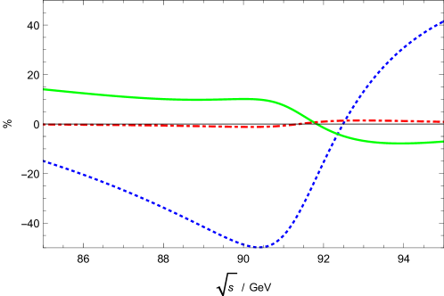
Figure 2: The ratio of the cross section containing all initial state corrections up to $O(a)$ (dotted line), to $O(a^{2})$ (full line), to $O(a^{3}{L}^{3})$ (dash-dotted line), normalized on all terms including also the $O(a^{3}{L})$ and $O(a^{4}{L}^{4})$ corrections to the cross section $e^{+}e^{-}\rightarrow\gamma^{*}/Z^{*}$ in the region of the $Z$-peak for $M_{Z}=91.1876\leavevmode\nobreak\ \mathrm{GeV}$ [62].

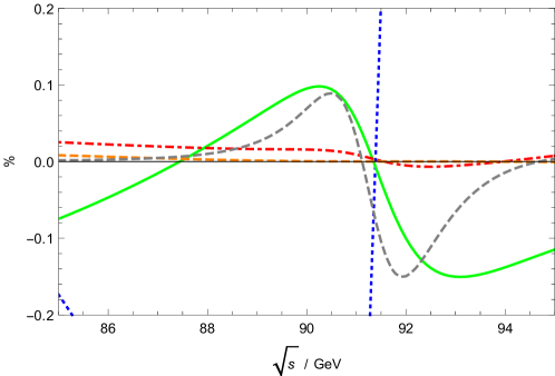
Figure 3: The ratio of the cross section containing all initial state corrections up to $O(a^{3}L^{3})$ (dotted line), to $O(a^{3}L^{2})$ (full line), to $O(a^{3}L)$ (dash-dotted line), universal terms contributing to $O(a^{3}L^{0})$ (dashed line), to $O(a^{4}L^{4})$ (long dashed line), normalized on all terms including also the $O(a^{3}L)$ and $O(a^{4}L^{4})$ corrections to the cross section $e^{+}e^{-}\rightarrow\gamma^{*}/Z^{*}$ in the region of the $Z$-peak for $M_{Z}=91.1876\leavevmode\nobreak\ \mathrm{GeV}$ [62].

In Figures 2 and 3 we compare the ratios of the three–loop terms with all contributions (25–37) in the kinematic region of $\sqrt{s}\in[85,95]\leavevmode\nobreak\ \mathrm{GeV}$.

The $O(a)$ radiative corrections are large and amount to $\sim\pm 40\%$, followed by the $O(a^{2})$ corrections, still varying from $+15\%$ to $-7\%$, cf. Figure 2. Already the leading term $O(a^{3}{L}^{3})$ yields only corrections at the 1% level. The $O(a^{3})$ corrections up to the $O(a^{3}L)$ term are significantly smaller and are illustrated in Figure 3.

	Fixed width		$s$ dep. width
	Peak	Width	Peak	Width
	(MeV)	(MeV)	(MeV)	(MeV)
$O(\alpha)$ correction	185.638	539.408	181.098	524.978
$O(\alpha^{2}L^{2})$:	– 96.894	–177.147	– 95.342	–176.235
$O(\alpha^{2}L)$:	6.982	22.695	6.841	21.896
$O(\alpha^{2})$:	0.176	– 2.218	0.174	– 2.001
$O(\alpha^{3}L^{3})$:	23.265	38.560	22.968	38.081
$O(\alpha^{3}L^{2})$:	– 1.507	– 1.888	– 1.491	– 1.881
$O(\alpha^{3}L)$:	– 0.152	0.105	– 0.151	– 0.084
$O(\alpha^{4}L^{4})$:	– 1.857	0.206	– 1.858	0.146
$O(\alpha^{4}L^{3})$:	0.131	– 0.071	0.132	– 0.065
$O(\alpha^{4}L^{2})$:	0.048	– 0.001	0.048	0.001
$O(\alpha^{5}L^{5})$:	0.142	– 0.218	0.144	– 0.212
$O(\alpha^{5}L^{4})$:	– 0.000	0.020	– 0.001	0.020
$O(\alpha^{5}L^{3})$:	– 0.008	0.009	– 0.008	0.008
$O(\alpha^{6}L^{6})$:	– 0.007	0.027	– 0.007	0.027
$O(\alpha^{6}L^{5})$:	– 0.001	0.000	– 0.001	0.000

Table 1: Shifts in the $Z$-mass and the width due to the different contributions to the ISR QED radiative corrections for a fixed width of $\Gamma_{Z}=2.4952\leavevmode\nobreak\ \mathrm{GeV}$ and $s$-dependent width using $M_{Z}=91.1876\leavevmode\nobreak\ \mathrm{GeV}$ [62] and $s_{0}=4m_{\tau}^{2}$, cf. [7].

Finally, we summarize the shifts of the $Z$ peak and the corrections to the $Z$ width, $\Gamma_{Z}$, by the different orders of the ISR radiative corrections in Table 8. Here we compare the results for the fixed and the $s$-dependent width [63]. In Figures 2 and 3 we depicted only the corrections up to $O(a^{3})$. The other corrections up to $O(a^{6}L^{5})$ are only illustrated w.r.t. its shift of the $Z$ mass and change of the $Z$ width since their behaviour is rather flat, yet they have an impact given the projected experimental resolutions. The difference to the results in Ref. [11] amounts to 4 MeV in $\Gamma_{Z}$,  [9, 10].

The relative shifts in adding the respective order can be positive or negative. at leading order $O(\alpha^{k}L^{k})$ the level of $100\leavevmode\nobreak\ \mathrm{keV}$ [64] is only undershoot at $O(\alpha^{5}L^{4})$. Even the $O(\alpha^{4}L^{2})$ corrections are of the order of $50\leavevmode\nobreak\ \mathrm{keV}$, while at $O(\alpha^{5}L^{3})$ the level of $10\leavevmode\nobreak\ \mathrm{keV}$ is reached. A missing link is still the $O(\alpha^{3})$ term, which can be estimated to be roughly of $O(30\leavevmode\nobreak\ \mathrm{keV})$, setting the frame of accuracy which is currently reached for the initial state corrections. The QED corrections to 3–loop order are still somewhat larger than the experimental resolution at the the FCC_ee [5] making the inclusion of also higher order subleading corrections necessary.

Furthermore, we remark that we have calculated the inclusive ISR corrections only, assuming that the experimental data are extrapolated to the full phase space and only a cut in $s^{\prime}$ is considered. The experimental requirements may be more ambitious, requiring more differential radiative corrections in the future. Due to different cuts, the corrections will turn out to be different and one has to carefully study all the cut dependencies. For a recent summary see [65]. From the size of the corrections it seems that 3- to 4-loop corrections have there to be provided too.

Numerical implementations for harmonic polylogarithms in Fortran needed for the radiators in $z$ space are given in [66] and [67], respectively.

6 Conclusions

We have calculated the QED initial state corrections to the annihilation process $e^{+}e^{-}\rightarrow\gamma^{*}/Z^{*}$ up to the terms $O(\alpha^{6}L^{5})$. They come next to the recently completed $O(\alpha^{2})$ corrections [8, 9, 10] and the well–known universal corrections $O((\alpha L)^{k})$, which were known to fifth order in explicit form in the non–singlet and singlet case [13, 14, 15, 16, 17, 18, 19, 20]. Here we included the first three logarithmic terms for the orders $O(\alpha^{3})$ to $O(\alpha^{5})$. The radiators are given by convolutions of splitting functions, the contributions to the Wilson coefficient of the massless Drell–Yan process and massive operator matrix elements. For the present corrections the massive OME $\Gamma_{\gamma e}^{(1)}$ had to be calculated newly. The other massive OMEs were given in [12] before. The corrections calculated in the present paper can be expressed in terms of harmonic polylogarithms, if one also allows for the argument $(1-x)$ in case of harmonic polylogarithms containing an index $i=-1$. In Mellin space the radiators can be represented in terms of harmonic sums and generalized harmonic sums. The present corrections may still miss terms of $O(30\leavevmode\nobreak\ \mathrm{keV})$ for both $\delta M_{Z}$ and $\delta\Gamma_{Z}$, which can be further improved by calculating the yet missing terms.

It is needless to say that by performing Mellin convolutions, using the quantities calculated in the present paper and the massless quantities available in the literature, one is now in the position to calculate all corrections of $O(\alpha^{k}L^{k}),O(\alpha^{k}L^{k-1})$ and $O(\alpha^{k}L^{k-2})$ for $k\geq 5$ straightforwardly. For the projected experimental accuracies in inclusive measurements at the FCC_ee they may not be needed beyond the orders already obtained.

Appendix A The Singularities of the Radiators in N space

For the use of complex contour integrals to calculate the radiative corrections the position of the singularities of the radiators in Mellin $N$ space in the complex plane have to be known.

In the case of harmonic sums, except for $S_{1}(N)$, it is known from their representation in terms of factorial series [68] that their singularities are given by the set $\{-n\leavevmode\nobreak\ |\leavevmode\nobreak\ n\in\mathbb{N}\}$. The sum $S_{1}(N)$ has a representation by the di-gamma function $\psi(N)$ for which the same holds.

A factorial series is given by

$$\Omega(x)=a_{0}+\sum_{k=0}^{\infty}\frac{a_{k+1}k!}{x(x+1)...(x+n)},\leavevmode\nobreak\ \leavevmode\nobreak\ \text{with}\leavevmode\nobreak\ \leavevmode\nobreak\ a_{i}\in\mathbb{C}.$$ (106)

The question to be answered is, which functions can be expanded into factorial series. The structure of (106) then provides the singularity structure for $x\in\mathbb{C}$. If a function $F(x)$ has the representation

$$F(x)=\int_{0}^{1}\leavevmode\nobreak\ dt\leavevmode\nobreak\ t^{x}\leavevmode\nobreak\ \varphi(t)$$ (107)

and the function $\varphi(t)$ can be expanded into a Taylor series in $(1-t)$, partial integration will then lead to a factorial series.

The radiators are expressed in terms of the following monomials

$$\frac{{\rm H}_{\vec{a}}(\xi)}{z^{k}(1-z)^{l}(1+z)^{m}},\leavevmode\nobreak\ \leavevmode\nobreak\ \leavevmode\nobreak\ l,m\in\mathbb{N},\leavevmode\nobreak\ \leavevmode\nobreak\ \leavevmode\nobreak\ k\in\{0,1\}$$ (108)

and $\xi\in\{z,1-z\}$, with $a_{i}\in\{0,1,-1\}$. To perform the Mellin transform of (108) suitable regularizations have to be chosen. Since the Mellin transform of the complete radiator exists and is unique, these partly arbitrary regularization terms add up to zero.

Now one has to assure that ${\rm H}_{\vec{a}}(\xi)$ can be expanded into a Taylor series in the variable $(1-z)$. This will require in case to change the argument from

$$z\leftrightarrow(1-z),$$ (109)

which is a valid operation on ${\rm H}_{\vec{a}}(\xi)$ on the expense of introducing the letter

$$\frac{1}{2-z}.$$ (110)

The structure in (108) can be generated by applying the following differential operator

$$\frac{{\rm H}_{\vec{a}}(z)}{z^{k}(1-z)^{l}(1+z)^{m}}=\frac{1}{z^{k}}\frac{d^{m+l}}{dx^{m+l}}{\rm H}_{\vec{c}_{1},\vec{c}_{2},\vec{a}}(z),$$ (111)

with

$$\{c_{11},...,c_{1m}\}=\{1,1,...,1\},\leavevmode\nobreak\ \leavevmode\nobreak\ \leavevmode\nobreak\ \leavevmode\nobreak\ \leavevmode\nobreak\ \{c_{21},...,c_{2l}\}=\{-1,-1,...,-1\}.$$ (112)

Furthermore, one has

$$\int_{0}^{1}dz\leavevmode\nobreak\ z^{N}\leavevmode\nobreak\ \frac{d}{dz}{\rm H}_{\vec{b}}(z)={\rm H}_{\vec{b}}(1)-N\int_{0}^{1}dz\leavevmode\nobreak\ z^{N-1}\leavevmode\nobreak\ {\rm H}_{\vec{b}}(z).$$ (113)

In this way and by the argument mapping (109) one arrives at valid functions $\varphi(t)$ allowing to expand into a factorial series. The above construction has now to be applied to all radiators and one finds the set of singularities to be a subset of $\{-n\leavevmode\nobreak\ |\leavevmode\nobreak\ n\in\mathbb{N}\cup\{-1\}\}$.

Appendix B The Radiators in N space

In the following we list all radiators which were calculated in the present paper in Mellin $N$ space for the use in Mellin space programs. The analytic continuation of the respective harmonic sums can be performed as described in Refs. [69, 70]. The package HarmonicSums allows to derive the asymptotic representation of these coefficients. Their recursion relations follow from the ones of the harmonic and generalized harmonic sums. As has been shown, there are no singularities right to $N=1$, which allows to perform the contour integral to $z$ space with the usual contour in the singlet–case, see e.g. [31], surrounding the singularities of the expression in the complex plane, cf. Appendix A.

The radiators $R_{ij}$ are related to the expansion coefficients from $c_{3,3}$ to $c_{6,5}$, also labeling the difference term (85) between the axial–vector and vector contributions, by

$$R_{ij}(N)={\rm\bf M}[c_{ij}(x)](N).$$ (114)

Alternating sums can be rewritten in terms of Mellin transforms such that the contribution due to $\ln(2)$ terms cancel, cf. [71]. We have also checked that the evanescent poles present in the above radiators up to $1/(N-4)$, cancel, leaving the rightmost pole $1/(N-1)$.

The analytic continuation is performed from the even integers. It can be obtained in the analyticity region for $N\rightarrow\mathbb{C}$ for both the harmonic sums and generalized harmonic sums expressing them for large values of $|N|$ by their asymptotic expansion and by using the recursion relations to map to finite values of $N\in\mathbb{C}$, [70].

The radiators in $N$ space are given by

$$R_{3,3} = \Biggl{\{}-\frac{16S_{1}Q_{56}}{27(N-1)N^{2}(N+1)^{2}(N+2)}+\frac{4Q_{96}}{27(N-1)N^{3}(N+1)^{3}(N+2)}$$ (115)

$$+\frac{64\big{(}6+11N+11N^{2}\big{)}S_{1}^{2}}{3N(N+1)}-\frac{256}{3}S_{1}^{3}\Biggr{\}}$$

$$R_{3,2} = \Biggl{\{}-\frac{16S_{2}Q_{51}}{9(N-1)N^{2}(N+1)^{2}(N+2)}-\frac{2Q_{159}}{27(N-1)^{2}N^{4}(N+1)^{4}(N+2)^{2}}$$ (116)

$$+\Biggl{[}\frac{8Q_{139}}{27(N-1)^{2}N^{3}(N+1)^{3}(N+2)^{2}}+\frac{256\big{(}6+11N+11N^{2}\big{)}S_{2}}{3N(N+1)}$$

$$-256S_{3}\Biggr{]}S_{1}+\Biggl{[}-\frac{32Q_{42}}{3(N-1)N^{2}(N+1)^{2}(N+2)}-512S_{2}\Biggr{]}S_{1}^{2}+\frac{512}{3}S_{1}^{3}$$

$$+\frac{64\big{(}6+11N+11N^{2}\big{)}S_{3}}{3N(N+1)}+\Biggl{[}\frac{32Q_{46}}{9(N-1)N^{2}(N+1)^{2}(N+2)}+768S_{1}^{2}$$

$$-\frac{64\big{(}36+59N+59N^{2}\big{)}S_{1}}{3N(N+1)}\Biggr{]}\zeta_{2}+\Biggl{[}\frac{32\big{(}6+11N+11N^{2}\big{)}}{3N(N+1)}-128S_{1}\Biggr{]}\zeta_{3}\Biggr{\}}$$

$$R_{3,1} = \Biggl{\{}\frac{\big{(}2+N+N^{2}\big{)}2^{8-N}[S_{2}(2)-S_{1,1}(1,2)-S_{1,1}(2,1)]Q_{36}}{3(N-3)(N-2)(N-1)^{2}N^{3}(N+1)(N+2)}$$ (117)

$$+\frac{16S_{2,1}Q_{54}}{9(N-1)N^{2}(N+1)^{2}(N+2)}+\frac{8S_{3}Q_{91}}{27(N-1)N^{2}(N+1)^{2}(N+2)}$$

$$+\frac{Q_{206}}{81(N-4)(N-3)(N-2)(N-1)^{2}N^{5}(N+1)^{5}(N+2)^{3}}$$

$$+\Biggl{[}\Biggl{[}-\frac{64S_{1}Q_{119}}{3(N-1)N^{2}(N+1)^{2}(N+2)^{2}}+\frac{32Q_{144}}{9(N-1)N^{3}(N+1)^{3}(N+2)^{2}}$$

$$+\frac{768(N+3)\big{(}2+N^{2}\big{)}S_{1}^{2}}{(N-1)N(N+1)(N+2)}\Biggr{]}S_{-2}+\Biggl{[}-\frac{32(N+3)\big{(}2+N^{2}\big{)}\big{(}6+13N+13N^{2}\big{)}}{3(N-1)N^{2}(N+1)^{2}(N+2)}$$

$$+\frac{128(N+3)\big{(}2+N^{2}\big{)}S_{1}}{(N-1)N(N+1)(N+2)}\Biggr{]}S_{-3}+\frac{64(N+3)\big{(}2+N^{2}\big{)}\big{(}6+13N+13N^{2}\big{)}S_{-2,1}}{(N-1)N^{2}(N+1)^{2}(N+2)}$$

$$-\frac{768(N+3)\big{(}2+N^{2}\big{)}S_{1}S_{-2,1}}{(N-1)N(N+1)(N+2)}+\Biggl{[}-\frac{32S_{1}Q_{119}}{3(N-1)N^{2}(N+1)^{2}(N+2)^{2}}$$

$$+\frac{16Q_{144}}{9(N-1)N^{3}(N+1)^{3}(N+2)^{2}}+\frac{384(N+3)\big{(}2+N^{2}\big{)}S_{1}^{2}}{(N-1)N(N+1)(N+2)}\Biggr{]}\zeta_{2}$$

$$+\Biggl{[}\frac{32(N+3)\big{(}2+N^{2}\big{)}\big{(}6+13N+13N^{2}\big{)}}{(N-1)N^{2}(N+1)^{2}(N+2)}-\frac{384(N+3)\big{(}2+N^{2}\big{)}S_{1}}{(N-1)N(N+1)(N+2)}\Biggr{]}\zeta_{3}\Biggr{]}(-1)^{N}$$

$$+\Biggl{[}-\frac{64S_{2,1}Q_{6}}{3(N-1)N(N+1)}+\frac{\big{(}2+N+N^{2}\big{)}2^{8-N}S_{1}(2)Q_{36}}{3(N-3)(N-2)(N-1)^{2}N^{3}(N+1)(N+2)}$$

$$-\frac{64S_{3}Q_{20}}{9(N-1)N}-\frac{16S_{2}Q_{132}}{27(N-1)N^{2}(N+1)^{2}(N+2)^{2}}$$

$$-\frac{8Q_{201}}{81(N-4)(N-3)(N-2)(N-1)^{2}N^{4}(N+1)^{4}(N+2)^{3}}-1152S_{2}^{2}-384S_{4}$$

$$-1280S_{3,1}-1024S_{-2,-1}+768S_{2,1,1}\Biggr{]}S_{1}+\Biggl{[}\frac{32S_{2}Q_{8}}{(N-1)N(N+1)}-256S_{2,1}$$

$$+\frac{16Q_{150}}{27(N-2)(N-1)^{2}N^{3}(N+1)^{3}(N+2)^{2}}\Biggr{]}S_{1}^{2}+\Biggl{[}-\frac{64Q_{40}}{27(N-1)N^{2}(N+1)^{2}(N+2)}$$

$$-128S_{2}\Biggr{]}S_{1}^{3}+\frac{512}{9}S_{1}^{4}+\Biggl{[}\frac{4Q_{175}}{27(N-2)(N-1)^{2}N^{3}(N+1)^{3}(N+2)^{2}}-384S_{3}\Biggr{]}S_{2}$$

$$+\frac{32\big{(}54+97N+97N^{2}\big{)}S_{2}^{2}}{3N(N+1)}+\frac{32(2+5N)(3+5N)S_{4}}{N(N+1)}+384S_{5}$$

$$+\Biggl{[}\Biggl{[}-\frac{256\big{(}2+3N+3N^{2}\big{)}}{N(N+1)}+1024S_{1}\Biggr{]}S_{-1}-256S_{-2,1}\Biggr{]}S_{-2}+640S_{-3}S_{-2}+192S_{-2}^{2}$$

$$+\frac{64\big{(}30+11N+11N^{2}\big{)}S_{3,1}}{3N(N+1)}-384S_{3,2}-384S_{4,1}+\frac{256\big{(}2+3N+3N^{2}\big{)}S_{-2,-1}}{N(N+1)}$$

$$-\frac{64\big{(}6+11N+11N^{2}\big{)}S_{2,1,1}}{N(N+1)}+768S_{3,1,1}-1024S_{-2,1,-2}$$

$$+\frac{3\big{(}2+N+N^{2}\big{)}2^{8+N}S_{1,1}\big{(}\frac{1}{2},1\big{)}}{(N-2)N(N+1)^{3}(N+2)}-\frac{128\big{(}2+N+N^{2}\big{)}^{2}S_{1}(2)S_{1,1}\big{(}\frac{1}{2},1\big{)}}{(N-1)N^{2}(N+1)^{2}(N+2)}$$

$$-\frac{128\big{(}2+N+N^{2}\big{)}^{2}(S_{1,2}\big{(}\frac{1}{2},2\big{)}-S_{1,1,1}\big{(}\frac{1}{2},1,2\big{)}-S_{1,1,1}\big{(}\frac{1}{2},2,1\big{)})}{(N-1)N^{2}(N+1)^{2}(N+2)}$$

$$+\Biggl{[}-\frac{32S_{1}^{2}Q_{12}}{3(N-1)N(N+1)}-\frac{4Q_{174}}{27(N-2)(N-1)^{2}N^{3}(N+1)^{3}(N+2)^{2}}$$

$$+\ln(2)\Biggl{[}-\frac{576\big{(}2+3N+3N^{2}\big{)}}{N(N+1)}+2304S_{1}\Biggr{]}$$

$$+128S_{1}^{3}+\Biggl{[}\frac{16Q_{133}}{27(N-1)N^{2}(N+1)^{2}(N+2)^{2}}+2432S_{2}\Biggr{]}S_{1}-\frac{64\big{(}19+30N+30N^{2}\big{)}S_{2}}{N(N+1)}$$

$$+576S_{3}+\Biggl{[}-\frac{128\big{(}2+3N+3N^{2}\big{)}}{N(N+1)}+512S_{1}\Biggr{]}S_{-1}+192S_{-2}+320S_{-3}$$

$$-640S_{-2,1}+\frac{64\big{(}2+N+N^{2}\big{)}^{2}S_{1}(2)}{(N-1)N^{2}(N+1)^{2}(N+2)}+160\zeta_{3}\Biggr{]}\zeta_{2}$$

$$+\Biggl{[}\frac{16\big{(}588+1171N+1171N^{2}\big{)}}{15N(N+1)}-\frac{6272}{5}S_{1}\Biggr{]}\zeta_{2}^{2}+\Biggl{[}\frac{64S_{1}Q_{34}}{3(N-1)N(N+1)}+512S_{1}^{2}$$

$$-\frac{16Q_{85}}{9(N-1)N^{2}(N+1)^{2}(N+2)}-192S_{2}+192S_{-2}\Biggr{]}\zeta_{3}-416\zeta_{5}\Biggr{\}}$$

$$R_{4,4} = \Biggl{\{}\frac{16S_{1}^{2}Q_{66}}{27(N-1)N^{2}(N+1)^{2}(N+2)}-\frac{8S_{1}Q_{103}}{27(N-1)N^{3}(N+1)^{3}(N+2)}$$ (118)

$$+\frac{Q_{160}}{27(N-1)^{2}N^{4}(N+1)^{4}(N+2)^{2}}-\frac{1024\big{(}1+2N+2N^{2}\big{)}S_{1}^{3}}{3N(N+1)}+\frac{512}{3}S_{1}^{4}\Biggr{\}}$$

$$R_{4,3} = \Biggl{\{}\frac{64S_{3}Q_{45}}{9(N-1)N^{2}(N+1)^{2}(N+2)}-\frac{16S_{2}Q_{104}}{27(N-1)N^{3}(N+1)^{3}(N+2)}$$ (119)

$$-\frac{2Q_{191}}{81(N-1)^{3}N^{5}(N+1)^{5}(N+2)^{3}}+\Biggl{[}\frac{64S_{2}Q_{69}}{27(N-1)N^{2}(N+1)^{2}(N+2)}$$

$$+\frac{16Q_{163}}{81(N-1)^{2}N^{4}(N+1)^{4}(N+2)^{2}}-\frac{1024\big{(}1+2N+2N^{2}\big{)}S_{3}}{N(N+1)}\Biggr{]}S_{1}$$

$$+\Biggl{[}-\frac{32Q_{141}}{27(N-1)^{2}N^{3}(N+1)^{3}(N+2)^{2}}-\frac{256\big{(}30+59N+59N^{2}\big{)}S_{2}}{3N(N+1)}+1024S_{3}\Biggr{]}S_{1}^{2}$$

$$+\Biggl{[}\frac{128Q_{49}}{9(N-1)N^{2}(N+1)^{2}(N+2)}+\frac{5120}{3}S_{2}\Biggr{]}S_{1}^{3}-\frac{1024}{3}S_{1}^{4}$$

$$+\Biggl{[}-\frac{64S_{1}Q_{70}}{27(N-1)N^{2}(N+1)^{2}(N+2)}+\frac{32Q_{102}}{27(N-1)N^{3}(N+1)^{3}(N+2)}$$

$$+\frac{512\big{(}21+38N+38N^{2}\big{)}S_{1}^{2}}{3N(N+1)}-\frac{7168}{3}S_{1}^{3}\Biggr{]}\zeta_{2}+\Biggl{[}\frac{32Q_{45}}{9(N-1)N^{2}(N+1)^{2}(N+2)}$$

$$-\frac{512\big{(}1+2N+2N^{2}\big{)}S_{1}}{N(N+1)}+512S_{1}^{2}\Biggr{]}\zeta_{3}\Biggr{\}}$$

$$R_{4,2} = \Biggl{\{}\frac{128\big{(}2+N+N^{2}\big{)}S_{-2,1}Q_{1}}{(N-1)N^{3}(N+1)^{2}(N+2)}+\frac{256S_{-2,-1}Q_{23}}{3(N-1)N(N+1)(N+2)}$$ (120)

$$-\frac{64S_{2,1,1}Q_{26}}{(N-1)N(N+1)(N+2)}+\frac{64S_{4}Q_{28}}{3(N-1)N(N+1)(N+2)}$$

$$+\frac{\big{(}2+N+N^{2}\big{)}\big{(}2+3N+3N^{2}\big{)}2^{7-N}(S_{2}(2)-S_{1,1}(1,2)-S_{1,1}(2,1))Q_{36}}{(N-3)(N-2)(N-1)^{2}N^{4}(N+1)^{2}(N+2)}$$

$$-\frac{64S_{3,1}Q_{38}}{3(N-1)N^{2}(N+1)^{2}(N+2)}+\frac{32S_{2}^{2}Q_{59}}{3(N-1)N^{2}(N+1)^{2}(N+2)}$$

$$+\frac{16S_{2,1}Q_{127}}{9(N-1)^{2}N^{3}(N+1)^{3}(N+2)}+\frac{16S_{3}Q_{157}}{27(N-1)^{2}N^{3}(N+1)^{3}(N+2)^{2}}$$

$$+\frac{Q_{212}}{162(N-4)(N-3)(N-2)(N-1)^{4}N^{6}(N+1)^{6}(N+2)^{5}}$$

$$+\Biggl{[}\frac{64S_{-2,1}Q_{122}}{(N-1)^{2}N^{3}(N+1)^{3}(N+2)^{2}}+\frac{32\big{(}2+N+N^{2}\big{)}Q_{156}}{9(N-1)^{2}N^{5}(N+1)^{6}(N+2)^{5}}$$

$$+\Biggl{[}\frac{512S_{1}^{2}Q_{118}}{3(N-1)N^{2}(N+1)^{2}(N+2)^{2}}-\frac{64S_{1}Q_{155}}{9(N-1)^{2}N^{3}(N+1)^{3}(N+2)^{2}}$$

$$+\frac{32Q_{187}}{9(N-1)^{2}N^{4}(N+1)^{4}(N+2)^{3}}-\frac{3072(N+3)\big{(}2+N^{2}\big{)}S_{1}^{3}}{(N-1)N(N+1)(N+2)}\Biggr{]}S_{-2}$$

$$+\Biggl{[}-\frac{32Q_{123}}{3(N-1)^{2}N^{3}(N+1)^{3}(N+2)^{2}}+\frac{512(N+3)\big{(}2+N^{2}\big{)}\big{(}3+7N+7N^{2}\big{)}S_{1}}{3(N-1)N^{2}(N+1)^{2}(N+2)}$$

$$-\frac{512(N+3)\big{(}2+N^{2}\big{)}S_{1}^{2}}{(N-1)N(N+1)(N+2)}\Biggr{]}S_{-3}-\frac{1024(N+3)\big{(}2+N^{2}\big{)}\big{(}3+7N+7N^{2}\big{)}S_{1}S_{-2,1}}{(N-1)N^{2}(N+1)^{2}(N+2)}$$

$$+\frac{3072(N+3)\big{(}2+N^{2}\big{)}S_{1}^{2}S_{-2,1}}{(N-1)N(N+1)(N+2)}+\Biggl{[}\frac{256S_{1}^{2}Q_{118}}{3(N-1)N^{2}(N+1)^{2}(N+2)^{2}}$$

$$-\frac{32S_{1}Q_{155}}{9(N-1)^{2}N^{3}(N+1)^{3}(N+2)^{2}}+\frac{16Q_{188}}{9(N-1)^{2}N^{4}(N+1)^{4}(N+2)^{3}}$$

$$-\frac{1536(N+3)\big{(}2+N^{2}\big{)}S_{1}^{3}}{(N-1)N(N+1)(N+2)}\Biggr{]}\zeta_{2}+\Biggl{[}\frac{32Q_{121}}{(N-1)^{2}N^{3}(N+1)^{3}(N+2)^{2}}$$

$$-\frac{512(N+3)\big{(}2+N^{2}\big{)}\big{(}3+7N+7N^{2}\big{)}S_{1}}{(N-1)N^{2}(N+1)^{2}(N+2)}+\frac{1536(N+3)\big{(}2+N^{2}\big{)}S_{1}^{2}}{(N-1)N(N+1)(N+2)}\Biggr{]}\zeta_{3}\Biggr{]}(-1)^{N}$$

$$+\Biggl{[}-\frac{\big{(}2+N+N^{2}\big{)}2^{9-N}(S_{2}(2)-S_{1,1}(1,2)-S_{1,1}(2,1))Q_{36}}{(N-3)(N-2)(N-1)^{2}N^{3}(N+1)(N+2)}$$

$$-\frac{64S_{2,1}Q_{58}}{9(N-1)N^{2}(N+1)^{2}(N+2)}-\frac{64S_{3}Q_{92}}{27(N-1)N^{2}(N+1)^{2}(N+2)}$$

$$-\frac{8Q_{209}}{81(N-4)(N-3)(N-2)(N-1)^{3}N^{5}(N+1)^{5}(N+2)^{3}}$$

$$+\Biggl{[}-\frac{16Q_{176}}{81(N-2)(N-1)^{2}N^{3}(N+1)^{3}(N+2)^{2}}+4096S_{3}\Biggr{]}S_{2}$$

$$-\frac{512\big{(}13+25N+25N^{2}\big{)}S_{2}^{2}}{N(N+1)}-\frac{256\big{(}24+89N+89N^{2}\big{)}S_{4}}{3N(N+1)}$$

$$-3072S_{5}-\frac{1024\big{(}21+19N+19N^{2}\big{)}S_{3,1}}{3N(N+1)}+3072S_{3,2}+3072S_{4,1}$$

$$-\frac{4096\big{(}3+5N+5N^{2}\big{)}S_{-2,-1}}{3N(N+1)}+\frac{3072\big{(}1+2N+2N^{2}\big{)}S_{2,1,1}}{N(N+1)}-6144S_{3,1,1}$$

$$+8192S_{-2,1,-2}+\Biggl{[}\frac{\big{(}2+N+N^{2}\big{)}\big{(}2+3N+3N^{2}\big{)}2^{7-N}Q_{36}}{(N-3)(N-2)(N-1)^{2}N^{4}(N+1)^{2}(N+2)}$$

$$+\frac{768\big{(}2+N+N^{2}\big{)}^{2}S_{1,1}\big{(}\frac{1}{2},1\big{)}}{(N-1)N^{2}(N+1)^{2}(N+2)}\Biggr{]}S_{1}(2)$$

$$-\frac{9\big{(}2+N+N^{2}\big{)}2^{9+N}S_{1,1}\big{(}\frac{1}{2},1\big{)}}{(N-2)N(N+1)^{3}(N+2)}$$

$$+\frac{768\big{(}2+N+N^{2}\big{)}^{2}(S_{1,2}\big{(}\frac{1}{2},2\big{)}-S_{1,1,1}\big{(}\frac{1}{2},1,2\big{)}-S_{1,1,1}\big{(}\frac{1}{2},2,1\big{)})}{(N-1)N^{2}(N+1)^{2}(N+2)}\Biggr{]}S_{1}$$

$$+\Biggl{[}\frac{256S_{3}Q_{19}}{9(N-1)N}-\frac{\big{(}2+N+N^{2}\big{)}2^{9-N}S_{1}(2)Q_{36}}{(N-3)(N-2)(N-1)^{2}N^{3}(N+1)(N+2)}$$

$$+\frac{32S_{2}Q_{134}}{27(N-1)N^{2}(N+1)^{2}(N+2)^{2}}+6656S_{2}^{2}+2048S_{4}$$

$$+\frac{16Q_{202}}{81(N-4)(N-3)(N-2)(N-1)^{2}N^{4}(N+1)^{4}(N+2)^{3}}$$

$$+\frac{256(N+3)\big{(}-1-9N+4N^{2}\big{)}S_{2,1}}{3(N-1)N(N+1)}+7168S_{3,1}+4096S_{-2,-1}-3072S_{2,1,1}\Biggr{]}S_{1}^{2}$$

$$+\Biggl{[}-\frac{256S_{2}Q_{5}}{(N-1)N(N+1)}-\frac{64Q_{151}}{27(N-2)(N-1)^{2}N^{3}(N+1)^{3}(N+2)^{2}}+1024S_{2,1}\Biggr{]}S_{1}^{3}$$

$$+\Biggl{[}\frac{128Q_{44}}{27(N-1)N^{2}(N+1)^{2}(N+2)}+512S_{2}\Biggr{]}S_{1}^{4}-\frac{2048}{9}S_{1}^{5}$$

$$+\Biggl{[}\frac{8Q_{194}}{81(N-2)(N-1)^{2}N^{4}(N+1)^{4}(N+2)^{3}}-\frac{256\big{(}24+47N+47N^{2}\big{)}S_{3}}{3N(N+1)}\Biggr{]}S_{2}$$

$$+512S_{3}^{2}+\frac{1536\big{(}1+2N+2N^{2}\big{)}S_{5}}{N(N+1)}+\Biggl{[}-\frac{64\big{(}2+N+N^{2}\big{)}Q_{116}}{(N-1)^{2}N^{4}(N+1)^{4}(N+2)^{3}}$$

$$+\Biggl{[}-\frac{128\big{(}2+N+N^{2}\big{)}Q_{1}}{(N-1)N^{3}(N+1)^{2}(N+2)}+2048S_{-2,1}\Biggr{]}S_{1}$$

$$+\Biggl{[}-\frac{256Q_{23}}{3(N-1)N(N+1)(N+2)}+\frac{4096\big{(}3+5N+5N^{2}\big{)}S_{1}}{3N(N+1)}-4096S_{1}^{2}\Biggr{]}S_{-1}$$

$$-\frac{1024\big{(}1+2N+2N^{2}\big{)}S_{-2,1}}{N(N+1)}\Biggr{]}S_{-2}+\Biggl{[}\frac{64\big{(}2+3N+3N^{2}\big{)}Q_{17}}{3(N-1)N^{2}(N+1)^{2}(N+2)}$$

$$+\frac{1024\big{(}3+N+N^{2}\big{)}S_{1}}{3N(N+1)}-1024S_{1}^{2}\Biggr{]}S_{-2}^{2}+\Biggl{[}-\frac{64\big{(}2+N+N^{2}\big{)}\big{(}6+9N+N^{3}\big{)}}{(N-1)N^{2}(N+1)^{3}(N+2)}$$

$$+\frac{256\big{(}2+N+N^{2}\big{)}^{2}S_{1}}{(N-1)N^{2}(N+1)^{2}(N+2)}+\Biggl{[}\frac{2560\big{(}1+2N+2N^{2}\big{)}}{N(N+1)}$$

$$-5120S_{1}\Biggr{]}S_{-2}\Biggr{]}S_{-3}+\frac{\big{(}2+N+N^{2}\big{)}^{2}(192S_{-4}+128S_{2,-2})}{(N-1)N^{2}(N+1)^{2}(N+2)}$$

$$-\frac{1536\big{(}1+2N+2N^{2}\big{)}(S_{3,2}+S_{4,1})}{N(N+1)}-\frac{256\big{(}2+N+N^{2}\big{)}^{2}S_{-3,1}}{(N-1)N^{2}(N+1)^{2}(N+2)}$$

$$+\frac{3072\big{(}1+2N+2N^{2}\big{)}S_{3,1,1}}{N(N+1)}-\frac{4096\big{(}1+2N+2N^{2}\big{)}S_{-2,1,-2}}{N(N+1)}$$

$$+\frac{192\big{(}2+N+N^{2}\big{)}^{2}\big{(}2+3N+3N^{2}\big{)}S_{1,1,1}\big{(}\frac{1}{2},1,2\big{)}}{(N-1)N^{3}(N+1)^{3}(N+2)}$$

$$+\frac{9\big{(}2+N+N^{2}\big{)}\big{(}2+3N+3N^{2}\big{)}2^{7+N}S_{1,1}\big{(}\frac{1}{2},1\big{)}}{(N-2)N^{2}(N+1)^{4}(N+2)}$$

$$-\frac{192\big{(}2+N+N^{2}\big{)}^{2}\big{(}2+3N+3N^{2}\big{)}}{(N-1)N^{3}(N+1)^{3}(N+2)}\biggl{(}S_{1}(2)S_{1,1}\big{(}\frac{1}{2},1\big{)}+S_{1,2}\big{(}\frac{1}{2},2\big{)}\biggr{)}$$

$$+\frac{192\big{(}2+N+N^{2}\big{)}^{2}\big{(}2+3N+3N^{2}\big{)}S_{1,1,1}\big{(}\frac{1}{2},2,1\big{)}}{(N-1)N^{3}(N+1)^{3}(N+2)}+\Biggl{[}\frac{256S_{1}^{3}Q_{11}}{3(N-1)N(N+1)}$$

$$-\frac{32S_{2}Q_{64}}{3(N-1)N^{2}(N+1)^{2}(N+2)}-\frac{4Q_{195}}{81(N-2)(N-1)^{2}N^{4}(N+1)^{4}(N+2)^{3}}$$

$$+\ln(2)\Biggl{[}-\frac{192Q_{23}}{(N-1)N(N+1)(N+2)}+\frac{3072\big{(}3+5N+5N^{2}\big{)}S_{1}}{N(N+1)}-9216S_{1}^{2}\Biggr{]}$$

$$+\Biggl{[}\frac{16Q_{177}}{81(N-2)(N-1)^{2}N^{3}(N+1)^{3}(N+2)^{2}}+\frac{512\big{(}87+151N+151N^{2}\big{)}S_{2}}{3N(N+1)}$$

$$-5632S_{3}+5120S_{-2,1}-\frac{384\big{(}2+N+N^{2}\big{)}^{2}S_{1}(2)}{(N-1)N^{2}(N+1)^{2}(N+2)}\Biggr{]}S_{1}$$

$$+\Biggl{[}-\frac{32Q_{135}}{27(N-1)N^{2}(N+1)^{2}(N+2)^{2}}-14848S_{2}\Biggr{]}S_{1}^{2}$$

$$-512S_{1}^{4}+\frac{256\big{(}33+58N+58N^{2}\big{)}S_{3}}{3N(N+1)}+\Biggl{[}-\frac{128Q_{23}}{3(N-1)N(N+1)(N+2)}$$

$$+\frac{2048\big{(}3+5N+5N^{2}\big{)}S_{1}}{3N(N+1)}-2048S_{1}^{2}\Biggr{]}S_{-1}+\Biggl{[}\frac{64Q_{39}}{3(N-1)N^{2}(N+1)^{2}(N+2)}$$

$$+\frac{1024\big{(}3+N+N^{2}\big{)}S_{1}}{3N(N+1)}-1024S_{1}^{2}\Biggr{]}S_{-2}+\Biggl{[}\frac{1280\big{(}1+2N+2N^{2}\big{)}}{N(N+1)}-2560S_{1}\Biggr{]}S_{-3}$$

$$-\frac{2560\big{(}1+2N+2N^{2}\big{)}S_{-2,1}}{N(N+1)}+\frac{96\big{(}2+N+N^{2}\big{)}^{2}\big{(}2+3N+3N^{2}\big{)}S_{1}(2)}{(N-1)N^{3}(N+1)^{3}(N+2)}$$

$$+\Biggl{[}\frac{128\big{(}21+34N+34N^{2}\big{)}}{3N(N+1)}-1792S_{1}\Biggr{]}\zeta_{3}\Biggr{]}\zeta_{2}+\Biggl{[}\frac{16Q_{74}}{15(N-1)N^{2}(N+1)^{2}(N+2)}$$

$$-\frac{256\big{(}387+770N+770N^{2}\big{)}S_{1}}{15N(N+1)}+\frac{33024}{5}S_{1}^{2}\Biggr{]}\zeta_{2}^{2}+\Biggl{[}-\frac{256S_{1}^{2}Q_{33}}{3(N-1)N(N+1)}$$

$$-\frac{16Q_{154}}{9(N-1)^{2}N^{3}(N+1)^{3}(N+2)^{2}}+\Biggl{[}\frac{256Q_{84}}{9(N-1)N^{2}(N+1)^{2}(N+2)}+2048S_{2}\Biggr{]}S_{1}$$

$$-2048S_{1}^{3}-\frac{128\big{(}24+47N+47N^{2}\big{)}S_{2}}{3N(N+1)}+512S_{3}+\Biggl{[}\frac{768\big{(}1+2N+2N^{2}\big{)}}{N(N+1)}$$

$$-1536S_{1}\Biggr{]}S_{-2}\Biggr{]}\zeta_{3}+128\zeta_{3}^{2}+\Biggl{[}-\frac{1664\big{(}1+2N+2N^{2}\big{)}}{N(N+1)}+3328S_{1}\Biggr{]}\zeta_{5}\Biggr{\}}$$

$$R_{5,5} = \Biggl{\{}\frac{16\big{(}6+13N+13N^{2}\big{)}S_{1}^{2}Q_{75}}{405(N-1)N^{3}(N+1)^{3}(N+2)}-\frac{64S_{1}^{3}Q_{77}}{135(N-1)N^{2}(N+1)^{2}(N+2)}$$ (121)

$$+\frac{\big{(}6+13N+13N^{2}\big{)}Q_{162}}{405(N-1)^{2}N^{5}(N+1)^{5}(N+2)^{2}}-\frac{4S_{1}Q_{167}}{405(N-1)^{2}N^{4}(N+1)^{4}(N+2)^{2}}$$

$$+\frac{1024\big{(}6+13N+13N^{2}\big{)}S_{1}^{4}}{9N(N+1)}-\frac{4096}{15}S_{1}^{5}\Biggr{\}}$$

$$R_{5,4} = \Biggl{\{}\frac{32\big{(}6+13N+13N^{2}\big{)}S_{3}Q_{50}}{27(N-1)N^{3}(N+1)^{3}(N+2)}-\frac{4S_{2}Q_{166}}{81(N-1)^{2}N^{4}(N+1)^{4}(N+2)^{2}}$$ (122)

$$+\frac{Q_{200}}{243(N-1)^{3}N^{6}(N+1)^{6}(N+2)^{3}}+\Biggl{[}-\frac{128S_{3}Q_{68}}{27(N-1)N^{2}(N+1)^{2}(N+2)}$$

$$+\frac{32S_{2}Q_{109}}{81(N-1)N^{3}(N+1)^{3}(N+2)}+\frac{4Q_{192}}{243(N-1)^{3}N^{5}(N+1)^{5}(N+2)^{3}}\Biggr{]}S_{1}$$

$$+\Biggl{[}-\frac{64S_{2}Q_{72}}{9(N-1)N^{2}(N+1)^{2}(N+2)}$$

$$-\frac{8Q_{169}}{243(N-1)^{2}N^{4}(N+1)^{4}(N+2)^{2}}+\frac{2048\big{(}6+13N+13N^{2}\big{)}S_{3}}{3N(N+1)}\Biggr{]}S_{1}^{2}$$

$$+\Biggl{[}\frac{64Q_{142}}{81(N-1)^{2}N^{3}(N+1)^{3}(N+2)^{2}}+\frac{8192\big{(}9+19N+19N^{2}\big{)}S_{2}}{9N(N+1)}-\frac{8192}{3}S_{3}\Biggr{]}S_{1}^{3}$$

$$+\Biggl{[}-\frac{128Q_{65}}{27(N-1)N^{2}(N+1)^{2}(N+2)}-4096S_{2}\Biggr{]}S_{1}^{4}+\frac{4096}{9}S_{1}^{5}$$

$$+\Biggl{[}\frac{128S_{1}^{2}Q_{76}}{27(N-1)N^{2}(N+1)^{2}(N+2)}-\frac{32S_{1}Q_{110}}{81(N-1)N^{3}(N+1)^{3}(N+2)}$$

$$+\frac{16Q_{164}}{81(N-1)^{2}N^{4}(N+1)^{4}(N+2)^{2}}-\frac{2048\big{(}48+95N+95N^{2}\big{)}S_{1}^{3}}{9N(N+1)}+$$

$$\frac{16384}{3}S_{1}^{4}\Biggr{]}\zeta_{2}+\Biggl{[}\frac{16\big{(}6+13N+13N^{2}\big{)}Q_{50}}{27(N-1)N^{3}(N+1)^{3}(N+2)}-\frac{64S_{1}Q_{68}}{27(N-1)N^{2}(N+1)^{2}(N+2)}$$

$$+\frac{1024\big{(}6+13N+13N^{2}\big{)}S_{1}^{2}}{3N(N+1)}-\frac{4096}{3}S_{1}^{3}\Biggr{]}\zeta_{3}\Biggr{\}}$$

$$R_{5,3} = \Biggl{\{}\frac{256S_{5}Q_{48}}{3(N-1)N^{2}(N+1)^{2}(N+2)}-\frac{256S_{3,2}Q_{48}}{3(N-1)N^{2}(N+1)^{2}(N+2)}$$ (123)

$$-\frac{256S_{4,1}Q_{48}}{3(N-1)N^{2}(N+1)^{2}(N+2)}+\frac{512S_{3,1,1}Q_{48}}{3(N-1)N^{2}(N+1)^{2}(N+2)}$$

$$+\frac{\big{(}2+N+N^{2}\big{)}2^{7-N}(S_{2}(2)-S_{1,1}(1,2)-S_{1,1}(2,1))Q_{36}Q_{52}}{27(N-3)(N-2)(N-1)^{3}N^{5}(N+1)^{3}(N+2)^{2}}$$

$$-\frac{2048S_{-2,1,-2}Q_{48}}{9(N-1)N^{2}(N+1)^{2}(N+2)}+\frac{\big{(}2+N+N^{2}\big{)}2^{7+N}S_{1,1}\big{(}\frac{1}{2},1\big{)}Q_{52}}{3(N-2)(N-1)N^{3}(N+1)^{5}(N+2)^{2}}$$

$$-\frac{64\big{(}2+N+N^{2}\big{)}^{2}S_{1}(2)S_{1,1}\big{(}\frac{1}{2},1\big{)}Q_{52}}{9(N-1)^{2}N^{4}(N+1)^{4}(N+2)^{2}}$$

$$-\frac{64\big{(}2+N+N^{2}\big{)}^{2}S_{1,2}\big{(}\frac{1}{2},2\big{)}Q_{52}}{9(N-1)^{2}N^{4}(N+1)^{4}(N+2)^{2}}+\frac{64\big{(}2+N+N^{2}\big{)}^{2}S_{1,1,1}\big{(}\frac{1}{2},1,2\big{)}Q_{52}}{9(N-1)^{2}N^{4}(N+1)^{4}(N+2)^{2}}$$

$$+\frac{64\big{(}2+N+N^{2}\big{)}^{2}S_{1,1,1}\big{(}\frac{1}{2},2,1\big{)}Q_{52}}{9(N-1)^{2}N^{4}(N+1)^{4}(N+2)^{2}}+\frac{128\big{(}2+N+N^{2}\big{)}S_{-2,1}Q_{87}}{9(N-1)^{2}N^{4}(N+1)^{4}(N+2)^{2}}$$

$$+\frac{512S_{-2,-1}Q_{96}}{27(N-1)N^{3}(N+1)^{3}(N+2)}-\frac{128S_{2,1,1}Q_{99}}{9(N-1)N^{3}(N+1)^{3}(N+2)}$$

$$-\frac{128S_{3,1}Q_{101}}{27(N-1)N^{3}(N+1)^{3}(N+2)}+\frac{64S_{4}Q_{106}}{27(N-1)N^{3}(N+1)^{3}(N+2)}$$

$$+\frac{64S_{2}^{2}Q_{107}}{27(N-1)N^{3}(N+1)^{3}(N+2)}+\frac{16S_{2,1}Q_{165}}{81(N-1)^{2}N^{4}(N+1)^{4}(N+2)^{2}}$$

$$+\frac{16S_{3}Q_{181}}{243(N-1)^{2}N^{4}(N+1)^{4}(N+2)^{2}}$$

$$+\frac{Q_{214}}{729(N-4)(N-3)(N-2)(N-1)^{4}N^{7}(N+1)^{7}(N+2)^{5}}$$

$$+\Biggl{[}\frac{128S_{-2,1}Q_{147}}{9(N-1)^{2}N^{4}(N+1)^{4}(N+2)^{2}}+\frac{32\big{(}2+N+N^{2}\big{)}Q_{182}}{81(N-1)^{2}N^{6}(N+1)^{7}(N+2)^{5}}$$

$$+\Biggl{[}-\frac{512S_{-2,1}Q_{126}}{9(N-1)^{2}N^{3}(N+1)^{3}(N+2)^{2}}-\frac{640\big{(}2+N+N^{2}\big{)}Q_{156}}{27(N-1)^{2}N^{5}(N+1)^{6}(N+2)^{5}}\Biggr{]}S_{1}$$

$$+\Biggl{[}-\frac{2048S_{1}^{3}Q_{120}}{9(N-1)N^{2}(N+1)^{2}(N+2)^{2}}+\frac{512S_{1}^{2}Q_{153}}{9(N-1)^{2}N^{3}(N+1)^{3}(N+2)^{2}}$$

$$-\frac{128S_{1}Q_{189}}{81(N-1)^{2}N^{4}(N+1)^{4}(N+2)^{3}}+\frac{32Q_{196}}{81(N-1)^{2}N^{5}(N+1)^{5}(N+2)^{3}}$$

$$+\frac{8192(N+3)\big{(}2+N^{2}\big{)}S_{1}^{4}}{(N-1)N(N+1)(N+2)}\Biggr{]}S_{-2}+\Biggl{[}\frac{256S_{1}Q_{98}}{27(N-1)^{2}N^{2}(N+1)^{3}(N+2)^{2}}$$

$$-\frac{64Q_{148}}{27(N-1)^{2}N^{4}(N+1)^{4}(N+2)^{2}}-\frac{1024(N+3)\big{(}2+N^{2}\big{)}\big{(}2+5N+5N^{2}\big{)}S_{1}^{2}}{(N-1)N^{2}(N+1)^{2}(N+2)}$$

$$+\frac{4096(N+3)\big{(}2+N^{2}\big{)}S_{1}^{3}}{3(N-1)N(N+1)(N+2)}\Biggr{]}S_{-3}+\frac{6144(N+3)\big{(}2+N^{2}\big{)}\big{(}2+5N+5N^{2}\big{)}S_{1}^{2}S_{-2,1}}{(N-1)N^{2}(N+1)^{2}(N+2)}$$

$$-\frac{8192(N+3)\big{(}2+N^{2}\big{)}S_{1}^{3}S_{-2,1}}{(N-1)N(N+1)(N+2)}+\Biggl{[}-\frac{1024S_{1}^{3}Q_{120}}{9(N-1)N^{2}(N+1)^{2}(N+2)^{2}}$$

$$+\frac{256S_{1}^{2}Q_{153}}{9(N-1)^{2}N^{3}(N+1)^{3}(N+2)^{2}}-\frac{64S_{1}Q_{190}}{81(N-1)^{2}N^{4}(N+1)^{4}(N+2)^{3}}$$

$$+\frac{16Q_{197}}{81(N-1)^{2}N^{5}(N+1)^{5}(N+2)^{3}}+\frac{4096(N+3)\big{(}2+N^{2}\big{)}S_{1}^{4}}{(N-1)N(N+1)(N+2)}\Biggr{]}\zeta_{2}$$

$$+\Biggl{[}-\frac{256S_{1}Q_{125}}{9(N-1)^{2}N^{3}(N+1)^{3}(N+2)^{2}}+\frac{64Q_{146}}{9(N-1)^{2}N^{4}(N+1)^{4}(N+2)^{2}}$$

$$+\frac{3072(N+3)\big{(}2+N^{2}\big{)}\big{(}2+5N+5N^{2}\big{)}S_{1}^{2}}{(N-1)N^{2}(N+1)^{2}(N+2)}-\frac{4096(N+3)\big{(}2+N^{2}\big{)}S_{1}^{3}}{(N-1)N(N+1)(N+2)}\Biggr{]}\zeta_{3}\Biggr{]}(-1)^{N}$$

$$+\Biggl{[}-\frac{2560\big{(}2+N+N^{2}\big{)}S_{-2,1}Q_{1}}{3(N-1)N^{3}(N+1)^{2}(N+2)}$$

$$-\frac{\big{(}2+N+N^{2}\big{)}\big{(}42+73N+73N^{2}\big{)}2^{10-N}S_{2}(2)Q_{36}}{27(N-3)(N-2)(N-1)^{2}N^{4}(N+1)^{2}(N+2)}$$

$$+\frac{\big{(}2+N+N^{2}\big{)}\big{(}42+73N+73N^{2}\big{)}2^{10-N}S_{1,1}(1,2)Q_{36}}{27(N-3)(N-2)(N-1)^{2}N^{4}(N+1)^{2}(N+2)}$$

$$+\frac{\big{(}2+N+N^{2}\big{)}\big{(}42+73N+73N^{2}\big{)}2^{10-N}S_{1,1}(2,1)Q_{36}}{27(N-3)(N-2)(N-1)^{2}N^{4}(N+1)^{2}(N+2)}$$

$$-\frac{512S_{3,1}Q_{53}}{9(N-1)N^{2}(N+1)^{2}(N+2)}-\frac{2048S_{-2,-1}Q_{56}}{27(N-1)N^{2}(N+1)^{2}(N+2)}$$

$$+\frac{512S_{2,1,1}Q_{57}}{9(N-1)N^{2}(N+1)^{2}(N+2)}-\frac{256S_{2}^{2}Q_{71}}{9(N-1)N^{2}(N+1)^{2}(N+2)}$$

$$-\frac{256S_{4}Q_{73}}{27(N-1)N^{2}(N+1)^{2}(N+2)}-\frac{128S_{2,1}Q_{128}}{81(N-1)^{2}N^{3}(N+1)^{3}(N+2)}$$

$$-\frac{128S_{3}Q_{161}}{243(N-1)^{2}N^{3}(N+1)^{3}(N+2)^{2}}$$

$$-\frac{4Q_{213}}{729(N-4)(N-3)(N-2)(N-1)^{4}N^{6}(N+1)^{6}(N+2)^{5}}$$

$$+\Biggl{[}-\frac{32Q_{198}}{729(N-2)(N-1)^{2}N^{4}(N+1)^{4}(N+2)^{3}}+\frac{2048\big{(}10+21N+21N^{2}\big{)}S_{3}}{N(N+1)}\Biggr{]}S_{2}$$

$$-4096S_{3}^{2}-\frac{2048\big{(}6+13N+13N^{2}\big{)}S_{5}}{N(N+1)}-\frac{2560\big{(}2+N+N^{2}\big{)}^{2}S_{2,-2}}{3(N-1)N^{2}(N+1)^{2}(N+2)}$$

$$+\frac{2048\big{(}6+13N+13N^{2}\big{)}S_{3,2}}{N(N+1)}+\frac{2048\big{(}6+13N+13N^{2}\big{)}S_{4,1}}{N(N+1)}$$

$$+\frac{5120\big{(}2+N+N^{2}\big{)}^{2}S_{-3,1}}{3(N-1)N^{2}(N+1)^{2}(N+2)}-\frac{4096\big{(}6+13N+13N^{2}\big{)}S_{3,1,1}}{N(N+1)}$$

$$+\frac{16384\big{(}6+13N+13N^{2}\big{)}S_{-2,1,-2}}{3N(N+1)}$$

$$+\Biggl{[}\frac{\big{(}2+N+N^{2}\big{)}2^{7-N}Q_{36}Q_{52}}{27(N-3)(N-2)(N-1)^{3}N^{5}(N+1)^{3}(N+2)^{2}}$$

$$+\frac{512\big{(}2+N+N^{2}\big{)}^{2}\big{(}42+73N+73N^{2}\big{)}S_{1,1}\big{(}\frac{1}{2},1\big{)}}{9(N-1)N^{3}(N+1)^{3}(N+2)}\Biggr{]}S_{1}(2)$$

$$-\frac{\big{(}2+N+N^{2}\big{)}\big{(}42+73N+73N^{2}\big{)}2^{10+N}S_{1,1}\big{(}\frac{1}{2},1\big{)}}{3(N-2)N^{2}(N+1)^{4}(N+2)}$$

$$+\frac{512\big{(}2+N+N^{2}\big{)}^{2}\big{(}42+73N+73N^{2}\big{)}S_{1,2}\big{(}\frac{1}{2},2\big{)}}{9(N-1)N^{3}(N+1)^{3}(N+2)}$$

$$-\frac{512\big{(}2+N+N^{2}\big{)}^{2}\big{(}42+73N+73N^{2}\big{)}S_{1,1,1}\big{(}\frac{1}{2},1,2\big{)}}{9(N-1)N^{3}(N+1)^{3}(N+2)}$$

$$-\frac{512\big{(}2+N+N^{2}\big{)}^{2}\big{(}42+73N+73N^{2}\big{)}S_{1,1,1}\big{(}\frac{1}{2},2,1\big{)}}{9(N-1)N^{3}(N+1)^{3}(N+2)}\Biggr{]}S_{1}$$

$$+\Biggl{[}\frac{7\big{(}2+N+N^{2}\big{)}2^{11-N}S_{2}(2)Q_{36}}{9(N-3)(N-2)(N-1)^{2}N^{3}(N+1)(N+2)}$$

$$-\frac{7\big{(}2+N+N^{2}\big{)}2^{11-N}S_{1,1}(1,2)Q_{36}}{9(N-3)(N-2)(N-1)^{2}N^{3}(N+1)(N+2)}$$

$$-\frac{7\big{(}2+N+N^{2}\big{)}2^{11-N}S_{1,1}(2,1)Q_{36}}{9(N-3)(N-2)(N-1)^{2}N^{3}(N+1)(N+2)}+\frac{256S_{2,1}Q_{63}}{27(N-1)N^{2}(N+1)^{2}(N+2)}$$

$$+\frac{256S_{3}Q_{89}}{9(N-1)N^{2}(N+1)^{2}(N+2)}+\frac{2048\big{(}18+37N+37N^{2}\big{)}S_{2}^{2}}{N(N+1)}$$

$$+\frac{8Q_{210}}{729(N-4)(N-3)(N-2)(N-1)^{3}N^{5}(N+1)^{5}(N+2)^{3}}$$

$$+\Biggl{[}\frac{64Q_{178}}{81(N-2)(N-1)^{2}N^{3}(N+1)^{3}(N+2)^{2}}-20480S_{3}\Biggr{]}S_{2}$$

$$+\frac{5120\big{(}2+7N+7N^{2}\big{)}S_{4}}{N(N+1)}+12288S_{5}+\frac{2048\big{(}18+23N+23N^{2}\big{)}S_{3,1}}{N(N+1)}-12288S_{3,2}$$

$$-12288S_{4,1}+\frac{8192\big{(}6+11N+11N^{2}\big{)}S_{-2,-1}}{3N(N+1)}-\frac{2048\big{(}6+13N+13N^{2}\big{)}S_{2,1,1}}{N(N+1)}$$

$$+24576S_{3,1,1}-32768S_{-2,1,-2}+\big{(}-\frac{\big{(}2+N+N^{2}\big{)}\big{(}42+73N+73N^{2}\big{)}2^{10-N}Q_{36}}{27(N-3)(N-2)(N-1)^{2}N^{4}(N+1)^{2}(N+2)}$$

$$-\frac{7168\big{(}2+N+N^{2}\big{)}^{2}S_{1,1}\big{(}\frac{1}{2},1\big{)}}{3(N-1)N^{2}(N+1)^{2}(N+2)}\big{)}S_{1}(2)+\frac{7\big{(}2+N+N^{2}\big{)}2^{11+N}S_{1,1}\big{(}\frac{1}{2},1\big{)}}{(N-2)N(N+1)^{3}(N+2)}$$

$$-\frac{7168\big{(}2+N+N^{2}\big{)}^{2}S_{1,2}\big{(}\frac{1}{2},2\big{)}}{3(N-1)N^{2}(N+1)^{2}(N+2)}+\frac{7168\big{(}2+N+N^{2}\big{)}^{2}S_{1,1,1}\big{(}\frac{1}{2},1,2\big{)}}{3(N-1)N^{2}(N+1)^{2}(N+2)}$$

$$+\frac{7168\big{(}2+N+N^{2}\big{)}^{2}S_{1,1,1}\big{(}\frac{1}{2},2,1\big{)}}{3(N-1)N^{2}(N+1)^{2}(N+2)}\Biggr{]}S_{1}^{2}+\Biggl{[}\frac{2048S_{2,1}Q_{3}}{9(N-1)N(N+1)}-\frac{2048S_{3}Q_{18}}{27(N-1)N}$$

$$+\frac{7\big{(}2+N+N^{2}\big{)}2^{11-N}S_{1}(2)Q_{36}}{9(N-3)(N-2)(N-1)^{2}N^{3}(N+1)(N+2)}-\frac{256S_{2}Q_{136}}{81(N-1)N^{2}(N+1)^{2}(N+2)^{2}}$$

$$-\frac{32Q_{203}}{243(N-4)(N-3)(N-2)(N-1)^{2}N^{4}(N+1)^{4}(N+2)^{3}}-24576S_{2}^{2}$$

$$-\frac{20480}{3}S_{4}-24576S_{3,1}-\frac{32768}{3}S_{-2,-1}+8192S_{2,1,1}\Biggr{]}S_{1}^{3}$$

$$+\Biggl{[}\frac{1024S_{2}Q_{9}}{3(N-1)N(N+1)}+\frac{128Q_{152}}{243(N-2)(N-1)^{2}N^{3}(N+1)^{3}(N+2)^{2}}-\frac{8192}{3}S_{2,1}\Biggr{]}S_{1}^{4}$$

$$+\Biggl{[}-\frac{512Q_{41}}{27(N-1)N^{2}(N+1)^{2}(N+2)}-\frac{4096}{3}S_{2}\Biggr{]}S_{1}^{5}+\frac{16384}{27}S_{1}^{6}$$

$$+\Biggl{[}-\frac{256S_{3}Q_{62}}{9(N-1)N^{2}(N+1)^{2}(N+2)}+\frac{8Q_{207}}{729(N-2)(N-1)^{3}N^{5}(N+1)^{5}(N+2)^{3}}\Biggr{]}S_{2}$$

$$+\frac{1024\big{(}6+13N+13N^{2}\big{)}S_{3}^{2}}{3N(N+1)}+\Biggl{[}-\frac{512S_{-2,1}Q_{48}}{9(N-1)N^{2}(N+1)^{2}(N+2)}$$

$$-\frac{64\big{(}2+N+N^{2}\big{)}Q_{145}}{9(N-1)^{2}N^{5}(N+1)^{5}(N+2)^{3}}+\Biggl{[}-\frac{128\big{(}2+N+N^{2}\big{)}Q_{115}}{9(N-1)^{2}N^{4}(N+1)^{4}(N+2)^{3}}$$

$$+\frac{4096\big{(}6+13N+13N^{2}\big{)}S_{-2,1}}{3N(N+1)}\Biggr{]}S_{1}+\Biggl{[}\frac{2560\big{(}2+N+N^{2}\big{)}Q_{1}}{3(N-1)N^{3}(N+1)^{2}(N+2)}-8192S_{-2,1}\Biggr{]}S_{1}^{2}$$

$$+\Biggl{[}\frac{2048S_{1}Q_{56}}{27(N-1)N^{2}(N+1)^{2}(N+2)}-\frac{512Q_{96}}{27(N-1)N^{3}(N+1)^{3}(N+2)}$$

$$-\frac{8192\big{(}6+11N+11N^{2}\big{)}S_{1}^{2}}{3N(N+1)}+\frac{32768}{3}S_{1}^{3}\Biggr{]}S_{-1}\Biggr{]}S_{-2}$$

$$+\Biggl{[}\frac{512S_{1}Q_{47}N(N+1)+128Q_{95}}{27(N-1)N^{3}(N+1)^{3}(N+2)}-\frac{2048\big{(}4+5N+5N^{2}\big{)}S_{1}^{2}}{N(N+1)}$$

$$+\frac{16384}{3}S_{1}^{3}\Biggr{]}S_{-2}^{2}+\Biggl{[}\frac{2560\big{(}2+N+N^{2}\big{)}S_{1}Q_{16}}{9(N-1)N^{3}(N+1)^{3}(N+2)}-\frac{64\big{(}2+N+N^{2}\big{)}Q_{88}}{9(N-1)^{2}N^{4}(N+1)^{4}(N+2)^{2}}$$

$$-\frac{5120\big{(}2+N+N^{2}\big{)}^{2}S_{1}^{2}}{3(N-1)N^{2}(N+1)^{2}(N+2)}+\Biggl{[}\frac{1280Q_{48}}{9(N-1)N^{2}(N+1)^{2}(N+2)}+20480S_{1}^{2}$$

$$-\frac{10240\big{(}6+13N+13N^{2}\big{)}S_{1}}{3N(N+1)}\Biggr{]}S_{-2}\Biggr{]}S_{-3}+\Biggl{[}\frac{320\big{(}2+N+N^{2}\big{)}^{2}\big{(}6+13N+13N^{2}\big{)}}{3(N-1)N^{3}(N+1)^{3}(N+2)}$$

$$-\frac{1280\big{(}2+N+N^{2}\big{)}^{2}S_{1}}{(N-1)N^{2}(N+1)^{2}(N+2)}\Biggr{]}S_{-4}+\frac{640\big{(}2+N+N^{2}\big{)}^{2}\big{(}6+13N+13N^{2}\big{)}S_{2,-2}}{9(N-1)N^{3}(N+1)^{3}(N+2)}$$

$$-\frac{1280\big{(}2+N+N^{2}\big{)}^{2}\big{(}6+13N+13N^{2}\big{)}S_{-3,1}}{9(N-1)N^{3}(N+1)^{3}(N+2)}+\Biggl{[}-\frac{1024S_{1}^{4}Q_{10}}{3(N-1)N(N+1)}$$

$$-\frac{1280S_{-2,1}Q_{48}}{9(N-1)N^{2}(N+1)^{2}(N+2)}+\frac{32\big{(}2+N+N^{2}\big{)}^{2}S_{1}(2)Q_{52}}{9(N-1)^{2}N^{4}(N+1)^{4}(N+2)^{2}}$$

$$+\frac{128S_{3}Q_{67}}{9(N-1)N^{2}(N+1)^{2}(N+2)}-\frac{128S_{2}Q_{105}}{27(N-1)N^{3}(N+1)^{3}(N+2)}$$

$$-\frac{4Q_{208}}{729(N-2)(N-1)^{3}N^{5}(N+1)^{5}(N+2)^{3}}+\ln(2)\Biggl{[}\frac{512S_{1}Q_{56}}{3(N-1)N^{2}(N+1)^{2}(N+2)}$$

$$-\frac{128Q_{96}}{3(N-1)N^{3}(N+1)^{3}(N+2)}-\frac{6144\big{(}6+11N+11N^{2}\big{)}S_{1}^{2}}{N(N+1)}+24576S_{1}^{3}\Biggr{]}$$

$$+\Biggl{[}\frac{256S_{2}Q_{79}}{27(N-1)N^{2}(N+1)^{2}(N+2)}+\frac{16Q_{199}}{729(N-2)(N-1)^{2}N^{4}(N+1)^{4}(N+2)^{3}}$$

$$-\frac{1024\big{(}78+151N+151N^{2}\big{)}S_{3}}{3N(N+1)}+\frac{10240\big{(}6+13N+13N^{2}\big{)}S_{-2,1}}{3N(N+1)}$$

$$-\frac{256\big{(}2+N+N^{2}\big{)}^{2}\big{(}42+73N+73N^{2}\big{)}S_{1}(2)}{9(N-1)N^{3}(N+1)^{3}(N+2)}\Biggr{]}S_{1}-\Biggl{[}\frac{2048\big{(}123+233N+233N^{2}\big{)}S_{2}}{3N(N+1)}$$

$$+\frac{64Q_{179}}{81(N-2)(N-1)^{2}N^{3}(N+1)^{3}(N+2)^{2}}-26624S_{3}+20480S_{-2,1}$$

$$-\frac{3584\big{(}2+N+N^{2}\big{)}^{2}S_{1}(2)}{3(N-1)N^{2}(N+1)^{2}(N+2)}\Biggr{]}S_{1}^{2}+\Biggl{[}\frac{256Q_{137}}{81(N-1)N^{2}(N+1)^{2}(N+2)^{2}}+\frac{167936}{3}S_{2}\Biggr{]}$$

$$\times S_{1}^{3}+\frac{4096}{3}S_{1}^{5}+\Biggl{[}\frac{1024S_{1}Q_{56}}{27(N-1)N^{2}(N+1)^{2}(N+2)}-\frac{256Q_{96}}{27(N-1)N^{3}(N+1)^{3}(N+2)}$$

$$-\frac{4096\big{(}6+11N+11N^{2}\big{)}S_{1}^{2}}{3N(N+1)}+\frac{16384}{3}S_{1}^{3}\Biggr{]}S_{-1}+\Biggl{[}\frac{2048S_{1}Q_{24}}{27N^{2}(N+1)^{2}}$$

$$+\frac{128Q_{94}}{27(N-1)N^{3}(N+1)^{3}(N+2)}-\frac{2048\big{(}4+5N+5N^{2}\big{)}S_{1}^{2}}{N(N+1)}+\frac{16384}{3}S_{1}^{3}\Biggr{]}S_{-2}$$

$$+\Biggl{[}\frac{640Q_{48}}{9(N-1)N^{2}(N+1)^{2}(N+2)}-\frac{5120\big{(}6+13N+13N^{2}\big{)}S_{1}}{3N(N+1)}+10240S_{1}^{2}\Biggr{]}S_{-3}$$

$$+\Biggl{[}\frac{64Q_{55}}{3(N-1)N^{2}(N+1)^{2}(N+2)}-\frac{1536\big{(}6+11N+11N^{2}\big{)}S_{1}}{N(N+1)}+9216S_{1}^{2}\Biggr{]}\zeta_{3}\Biggr{]}\zeta_{2}$$

$$+\Biggl{[}-\frac{256S_{1}Q_{82}}{135(N-1)N^{2}(N+1)^{2}(N+2)}+\frac{32Q_{112}}{135(N-1)N^{3}(N+1)^{3}(N+2)}$$

$$+\frac{512\big{(}1020+2081N+2081N^{2}\big{)}S_{1}^{2}}{15N(N+1)}-\frac{69632}{3}S_{1}^{3}\Biggl{]}\zeta_{2}^{2}+\Biggr{[}\frac{2048S_{1}^{3}Q_{32}}{9(N-1)N(N+1)}$$

$$-\frac{128S_{2}Q_{62}}{9(N-1)N^{2}(N+1)^{2}(N+2)}-\frac{16Q_{180}}{81(N-1)^{2}N^{4}(N+1)^{4}(N+2)^{2}}$$

$$+\Biggl{[}\frac{64Q_{158}}{81(N-1)^{2}N^{3}(N+1)^{3}(N+2)^{2}}+\frac{1024\big{(}10+21N+21N^{2}\big{)}S_{2}}{N(N+1)}-4096S_{3}\Biggr{]}S_{1}$$

$$+\Biggl{[}-\frac{256Q_{93}}{27(N-1)N^{2}(N+1)^{2}(N+2)}-10240S_{2}\Biggr{]}S_{1}^{2}+\frac{16384}{3}S_{1}^{4}$$

$$+\frac{1024\big{(}6+13N+13N^{2}\big{)}S_{3}}{3N(N+1)}+\Biggl{[}\frac{128Q_{48}}{3(N-1)N^{2}(N+1)^{2}(N+2)}$$

$$-\frac{1024\big{(}6+13N+13N^{2}\big{)}S_{1}}{N(N+1)}+6144S_{1}^{2}\Biggr{]}S_{-2}\Biggr{]}\zeta_{3}$$

$$+\Biggl{[}\frac{256\big{(}6+13N+13N^{2}\big{)}}{3N(N+1)}-1024S_{1}\Biggr{]}\zeta_{3}^{2}+\Biggl{[}-\frac{832Q_{48}}{9(N-1)N^{2}(N+1)^{2}(N+2)}$$

$$+\frac{6656\big{(}6+13N+13N^{2}\big{)}S_{1}}{3N(N+1)}-13312S_{1}^{2}\Biggr{]}\zeta_{5}\Biggr{\}},$$

$$R_{6,6} = \Biggl{\{}\frac{128S_{1}^{4}Q_{80}}{405(N-1)N^{2}(N+1)^{2}(N+2)}$$ (125)

$$-\frac{256S_{1}^{3}Q_{108}}{405(N-1)N^{3}(N+1)^{3}(N+2)}+\frac{16S_{1}^{2}Q_{171}}{3645(N-1)^{2}N^{4}(N+1)^{4}(N+2)^{2}}$$

$$-\frac{16S_{1}Q_{183}}{3645(N-1)^{2}N^{5}(N+1)^{5}(N+2)^{2}}+\frac{Q_{204}}{7290(N-1)^{3}N^{6}(N+1)^{6}(N+2)^{3}}$$

$$-\frac{16384\big{(}3+7N+7N^{2}\big{)}S_{1}^{5}}{45N(N+1)}+\frac{16384}{45}S_{1}^{6}\Biggr{\}}$$

$$R_{6,5} = \Biggl{\{}\frac{16S_{3}Q_{168}}{405(N-1)^{2}N^{4}(N+1)^{4}(N+2)^{2}}-\frac{16S_{2}Q_{184}}{1215(N-1)^{2}N^{5}(N+1)^{5}(N+2)^{2}}$$ (126)

$$+\frac{Q_{211}}{7290(N-1)^{4}N^{7}(N+1)^{7}(N+2)^{4}}+\Biggl{[}-\frac{128S_{3}Q_{111}}{405(N-1)N^{3}(N+1)^{3}(N+2)}$$

$$+\frac{32S_{2}Q_{172}}{1215(N-1)^{2}N^{4}(N+1)^{4}(N+2)^{2}}+\frac{8Q_{205}}{3645(N-1)^{3}N^{6}(N+1)^{6}(N+2)^{3}}\Biggr{]}S_{1}$$

$$+\Biggl{[}\frac{256S_{3}Q_{81}}{135(N-1)N^{2}(N+1)^{2}(N+2)}-\frac{256S_{2}Q_{113}}{405(N-1)N^{3}(N+1)^{3}(N+2)}$$

$$-\frac{8Q_{193}}{3645(N-1)^{3}N^{5}(N+1)^{5}(N+2)^{3}}\Biggr{]}S_{1}^{2}+\Biggl{[}\frac{512S_{2}Q_{78}}{45(N-1)N^{2}(N+1)^{2}(N+2)}$$

$$+\frac{32Q_{170}}{405(N-1)^{2}N^{4}(N+1)^{4}(N+2)^{2}}-\frac{32768\big{(}3+7N+7N^{2}\big{)}S_{3}}{9N(N+1)}\Biggr{]}S_{1}^{3}$$

$$-\Biggl{[}\frac{256Q_{143}}{405(N-1)^{2}N^{3}(N+1)^{3}(N+2)^{2}}+\frac{4096\big{(}42+95N+95N^{2}\big{)}S_{2}}{9N(N+1)}$$

$$-\frac{16384}{3}S_{3}\Biggr{]}S_{1}^{4}+\Biggl{[}\frac{512Q_{61}}{45(N-1)N^{2}(N+1)^{2}(N+2)}+\frac{114688}{15}S_{2}\Biggr{]}S_{1}^{5}-\frac{16384}{45}S_{1}^{6}$$

$$+\Biggl{[}-\frac{256S_{1}^{3}Q_{83}}{135(N-1)N^{2}(N+1)^{2}(N+2)}+\frac{128S_{1}^{2}Q_{114}}{405(N-1)N^{3}(N+1)^{3}(N+2)}$$

$$-\frac{16S_{1}Q_{173}}{1215(N-1)^{2}N^{4}(N+1)^{4}(N+2)^{2}}+\frac{8Q_{185}}{1215(N-1)^{2}N^{5}(N+1)^{5}(N+2)^{2}}$$

$$+\frac{8192\big{(}27+58N+58N^{2}\big{)}S_{1}^{4}}{9N(N+1)}-\frac{49152}{5}S_{1}^{5}\Biggr{]}\zeta_{2}+\Biggl{[}\frac{128S_{1}^{2}Q_{81}}{135(N-1)N^{2}(N+1)^{2}(N+2)}$$

$$-\frac{64S_{1}Q_{111}}{405(N-1)N^{3}(N+1)^{3}(N+2)}+\frac{8Q_{168}}{405(N-1)^{2}N^{4}(N+1)^{4}(N+2)^{2}}$$

$$-\frac{16384\big{(}3+7N+7N^{2}\big{)}S_{1}^{3}}{9N(N+1)}+\frac{8192}{3}S_{1}^{4}\Biggr{]}\zeta_{3}\Biggr{\}}$$

$$R_{3,1,\Delta} = \Biggl{\{}\frac{32\big{(}6+13N+13N^{2}\big{)}Q_{29}}{3(N-1)N^{4}(N+1)^{3}}+\Biggl{[}\Biggl{[}-\frac{128\big{(}6+13N+13N^{2}\big{)}Q_{2}}{3(N-1)N^{3}(N+1)^{3}}+\frac{128S_{1}Q_{22}}{(N-1)N^{2}(N+1)^{2}}$$ (127)

$$-\frac{1536S_{1}^{2}}{N-1}\Biggr{]}S_{-2}+\Biggl{[}\frac{64\big{(}6+13N+13N^{2}\big{)}}{3(N-1)N(N+1)}-\frac{256S_{1}}{N-1}\Biggr{]}S_{-3}-\frac{128\big{(}6+13N+13N^{2}\big{)}S_{-2,1}}{(N-1)N(N+1)}$$

$$+\frac{1536S_{1}S_{-2,1}}{N-1}+\Biggl{[}-\frac{64\big{(}6+13N+13N^{2}\big{)}Q_{2}}{3(N-1)N^{3}(N+1)^{3}}+\frac{64S_{1}Q_{22}}{(N-1)N^{2}(N+1)^{2}}-\frac{768S_{1}^{2}}{N-1}\Biggr{]}\zeta_{2}$$

$$+\Biggl{[}-\frac{64\big{(}6+13N+13N^{2}\big{)}}{(N-1)N(N+1)}+\frac{768S_{1}}{N-1}\Biggr{]}\zeta_{3}\Biggr{]}(-1)^{N}$$

$$+\Biggl{[}-\frac{128Q_{29}}{(N-1)N^{3}(N+1)^{2}}-\frac{128S_{2}Q_{35}}{3(N-1)N^{2}(N+1)^{2}}-\frac{512S_{3}}{(N-1)N(N+1)}$$

$$-\frac{512S_{2,1}}{(N-1)N(N+1)}\Biggr{]}S_{1}+\frac{64\big{(}6+13N+13N^{2}\big{)}\big{(}2-N^{2}+N^{4}\big{)}S_{2}}{3(N-1)N^{3}(N+1)^{2}}$$

$$+\frac{128\big{(}6+13N+13N^{2}\big{)}S_{3}}{3(N-1)N^{2}(N+1)^{2}}+\frac{512S_{1}^{2}S_{2}}{(N-1)N(N+1)}$$

$$+\frac{128\big{(}6+13N+13N^{2}\big{)}S_{2,1}}{3(N-1)N^{2}(N+1)^{2}}+\Biggl{[}-\frac{64\big{(}6+13N+13N^{2}\big{)}\big{(}2-N^{2}+N^{4}\big{)}}{3(N-1)N^{3}(N+1)^{2}}$$

$$+\frac{128S_{1}Q_{35}}{3(N-1)N^{2}(N+1)^{2}}-\frac{512S_{1}^{2}}{(N-1)N(N+1)}\Biggr{]}\zeta_{2}$$

$$+\Biggl{[}-\frac{128\big{(}6+13N+13N^{2}\big{)}}{(N-1)N^{2}(N+1)^{2}}+\frac{1536S_{1}}{(N-1)N(N+1)}\Biggr{]}\zeta_{3}\Biggr{\}}$$

$$R_{4,2,\Delta} = \Biggl{\{}\frac{64\big{(}2-N^{2}+N^{4}\big{)}S_{2}Q_{27}}{3(N-1)^{2}N^{3}(N+1)^{2}(N+2)}+\frac{128S_{3}Q_{27}}{3(N-1)^{2}N^{2}(N+1)^{2}(N+2)}$$ (128)

$$+\frac{128S_{2,1}Q_{27}}{3(N-1)^{2}N^{2}(N+1)^{2}(N+2)}+\frac{32Q_{27}Q_{29}}{3(N-1)^{2}N^{4}(N+1)^{3}(N+2)}$$

$$+\Biggl{[}-\frac{128S_{-2,1}Q_{27}}{(N-1)^{2}N(N+1)(N+2)}+\Biggl{[}-\frac{2048S_{1}^{2}Q_{15}}{(N-1)N^{2}(N+1)^{2}}+\frac{6144S_{1}^{3}}{N-1}$$

$$-\frac{128(Q_{2}Q_{27}-Q_{90}S_{1})}{3(N-1)^{2}N^{3}(N+1)^{3}(N+2)}\Biggr{]}S_{-2}$$

$$+\Biggl{[}\frac{64Q_{27}}{3(N-1)^{2}N(N+1)(N+2)}-\frac{1024\big{(}3+7N+7N^{2}\big{)}S_{1}}{3(N-1)N(N+1)}$$

$$+\frac{1024S_{1}^{2}}{N-1}\Biggr{]}S_{-3}+\frac{2048\big{(}3+7N+7N^{2}\big{)}S_{1}S_{-2,1}}{(N-1)N(N+1)}-\frac{6144S_{1}^{2}S_{-2,1}}{N-1}+\Biggl{[}$$

$$-\frac{1024S_{1}^{2}Q_{15}}{(N-1)N^{2}(N+1)^{2}}-\frac{64(Q_{2}Q_{27}-S_{1}Q_{90})}{3(N-1)^{2}N^{3}(N+1)^{3}(N+2)}$$

$$+\frac{3072S_{1}^{3}}{N-1}\Biggr{]}\zeta_{2}+\Biggl{[}-\frac{64Q_{27}}{(N-1)^{2}N(N+1)(N+2)}+\frac{1024\big{(}3+7N+7N^{2}\big{)}S_{1}}{(N-1)N(N+1)}$$

$$-\frac{3072S_{1}^{2}}{N-1}\Biggr{]}\zeta_{3}\Biggr{]}(-1)^{N}+\Biggl{[}-\frac{512\big{(}3+7N+7N^{2}\big{)}Q_{29}}{3(N-1)N^{4}(N+1)^{3}}-\frac{128S_{2}Q_{86}}{3(N-1)^{2}N^{3}(N+1)^{2}(N+2)}$$

$$-\frac{2048\big{(}3+7N+7N^{2}\big{)}S_{3}}{3(N-1)N^{2}(N+1)^{2}}-\frac{2048\big{(}3+7N+7N^{2}\big{)}S_{2,1}}{3(N-1)N^{2}(N+1)^{2}}\Biggr{]}S_{1}+\Biggl{[}\frac{512Q_{29}}{(N-1)N^{3}(N+1)^{2}}$$

$$+\frac{1024S_{2}Q_{31}}{3(N-1)N^{2}(N+1)^{2}}+\frac{2048S_{3}}{(N-1)N(N+1)}+\frac{2048S_{2,1}}{(N-1)N(N+1)}\Biggr{]}S_{1}^{2}$$

$$-\frac{2048S_{1}^{3}S_{2}}{(N-1)N(N+1)}+\Biggl{[}-\frac{64\big{(}2-N^{2}+N^{4}\big{)}Q_{27}}{3(N-1)^{2}N^{3}(N+1)^{2}(N+2)}-\frac{1024S_{1}^{2}Q_{31}}{3(N-1)N^{2}(N+1)^{2}}$$

$$+\frac{128S_{1}Q_{86}}{3(N-1)^{2}N^{3}(N+1)^{2}(N+2)}+\frac{2048S_{1}^{3}}{(N-1)N(N+1)}\Biggr{]}\zeta_{2}$$

$$+\Biggl{[}-\frac{128Q_{27}}{(N-1)^{2}N^{2}(N+1)^{2}(N+2)}+\frac{2048\big{(}3+7N+7N^{2}\big{)}S_{1}}{(N-1)N^{2}(N+1)^{2}}$$

$$-\frac{6144S_{1}^{2}}{(N-1)N(N+1)}\Biggr{]}\zeta_{3}\Biggr{\}}$$

$$R_{5,3,\Delta} = \frac{64Q_{29}Q_{100}}{27(N-1)^{2}N^{6}(N+1)^{5}(N+2)}+\frac{128\big{(}2-N^{2}+N^{4}\big{)}S_{2}Q_{100}}{27(N-1)^{2}N^{5}(N+1)^{4}(N+2)}$$ (129)

$$+\frac{256S_{3}Q_{100}}{27(N-1)^{2}N^{4}(N+1)^{4}(N+2)}+\frac{256S_{2,1}Q_{100}}{27(N-1)^{2}N^{4}(N+1)^{4}(N+2)}$$

$$+\Biggl{[}\frac{1024S_{1}S_{-2,1}Q_{60}}{9(N-1)^{2}N^{2}(N+1)^{2}(N+2)}-\frac{256S_{-2,1}Q_{100}}{9(N-1)^{2}N^{3}(N+1)^{3}(N+2)}$$

$$+\Biggl{[}\frac{4096S_{1}^{3}Q_{25}}{3(N-1)N^{2}(N+1)^{2}}-\frac{1024S_{1}^{2}Q_{97}}{9(N-1)^{2}N^{3}(N+1)^{3}(N+2)}$$

$$-\frac{256Q_{2}Q_{100}}{27(N-1)^{2}N^{5}(N+1)^{5}(N+2)}+\frac{256S_{1}Q_{140}}{27(N-1)^{2}N^{4}(N+1)^{4}(N+2)}-\frac{16384S_{1}^{4}}{N-1}\Biggr{]}S_{-2}$$

$$+\Biggl{[}-\frac{512S_{1}Q_{60}}{27(N-1)^{2}N^{2}(N+1)^{2}(N+2)}+\frac{128Q_{100}}{27(N-1)^{2}N^{3}(N+1)^{3}(N+2)}$$

$$+\frac{2048\big{(}2+5N+5N^{2}\big{)}S_{1}^{2}}{(N-1)N(N+1)}-\frac{8192S_{1}^{3}}{3(N-1)}\Biggr{]}S_{-3}$$

$$-\frac{12288\big{(}2+5N+5N^{2}\big{)}S_{1}^{2}S_{-2,1}}{(N-1)N(N+1)}+\frac{16384S_{1}^{3}S_{-2,1}}{N-1}+\Biggl{[}\frac{2048S_{1}^{3}Q_{25}}{3(N-1)N^{2}(N+1)^{2}}$$

$$-\frac{512S_{1}^{2}Q_{97}}{9(N-1)^{2}N^{3}(N+1)^{3}(N+2)}-\frac{128Q_{2}Q_{100}}{27(N-1)^{2}N^{5}(N+1)^{5}(N+2)}$$

$$+\frac{128S_{1}Q_{140}}{27(N-1)^{2}N^{4}(N+1)^{4}(N+2)}-\frac{8192S_{1}^{4}}{N-1}\Biggr{]}\zeta_{2}+\Biggl{[}\frac{512S_{1}Q_{60}}{9(N-1)^{2}N^{2}(N+1)^{2}(N+2)}$$

$$-\frac{128Q_{100}}{9(N-1)^{2}N^{3}(N+1)^{3}(N+2)}-\frac{6144\big{(}2+5N+5N^{2}\big{)}S_{1}^{2}}{(N-1)N(N+1)}+\frac{8192S_{1}^{3}}{N-1}\Biggr{]}\zeta_{3}\Biggr{]}(-1)^{N}$$

$$+\Biggl{[}-\frac{256Q_{29}Q_{60}}{27(N-1)^{2}N^{5}(N+1)^{4}(N+2)}-\frac{1024S_{3}Q_{60}}{27(N-1)^{2}N^{3}(N+1)^{3}(N+2)}$$

$$-\frac{1024S_{2,1}Q_{60}}{27(N-1)^{2}N^{3}(N+1)^{3}(N+2)}-\frac{256S_{2}Q_{149}}{27(N-1)^{2}N^{4}(N+1)^{4}(N+2)}\Biggr{]}S_{1}$$

$$+\Biggl{[}\frac{1024\big{(}2+5N+5N^{2}\big{)}Q_{29}}{(N-1)N^{4}(N+1)^{3}}+\frac{1024S_{2}Q_{124}}{27(N-1)^{2}N^{3}(N+1)^{3}(N+2)}$$

$$+\frac{4096\big{(}2+5N+5N^{2}\big{)}S_{3}}{(N-1)N^{2}(N+1)^{2}}+\frac{4096\big{(}2+5N+5N^{2}\big{)}S_{2,1}}{(N-1)N^{2}(N+1)^{2}}\Biggr{]}S_{1}^{2}$$

$$+\Biggl{[}-\frac{4096Q_{29}}{3(N-1)N^{3}(N+1)^{2}}-\frac{4096S_{2}Q_{30}}{3(N-1)N^{2}(N+1)^{2}}$$

$$-\frac{16384S_{3}}{3(N-1)N(N+1)}-\frac{16384S_{2,1}}{3(N-1)N(N+1)}\Biggr{]}S_{1}^{3}$$

$$+\frac{16384S_{1}^{4}S_{2}}{3(N-1)N(N+1)}+\Biggl{[}\frac{4096S_{1}^{3}Q_{30}}{3(N-1)N^{2}(N+1)^{2}}$$

$$-\frac{128\big{(}2-N^{2}+N^{4}\big{)}Q_{100}}{27(N-1)^{2}N^{5}(N+1)^{4}(N+2)}-\frac{1024S_{1}^{2}Q_{124}}{27(N-1)^{2}N^{3}(N+1)^{3}(N+2)}$$

$$+\frac{256S_{1}Q_{149}}{27(N-1)^{2}N^{4}(N+1)^{4}(N+2)}-\frac{16384S_{1}^{4}}{3(N-1)N(N+1)}\Biggr{]}\zeta_{2}$$

$$+\Biggl{[}\frac{1024S_{1}Q_{60}}{9(N-1)^{2}N^{3}(N+1)^{3}(N+2)}-\frac{256Q_{100}}{9(N-1)^{2}N^{4}(N+1)^{4}(N+2)}$$

$$-\frac{12288\big{(}2+5N+5N^{2}\big{)}S_{1}^{2}}{(N-1)N^{2}(N+1)^{2}}+\frac{16384S_{1}^{3}}{(N-1)N(N+1)}\Biggr{]}\zeta_{3}.$$

The polynomials $Q_{k}|_{k=1}^{213}$ are to long to be displayed here and they are given in an ancillary file to this paper.

Acknowledgments.
We would like to thank P. Marquard and C. Schneider for discussions. This project has received funding from the European Union’s Horizon 2020 research and innovation programme under the Marie Sklodowska-Curie grant agreement No. 764850, SAGEX, COST action CA16201: Unraveling new physics at the LHC through the precision frontier, and Austrian Science Fund (FWF) grant SFB F50 (F5009-N15). The large formulae were tyosetted by using SigmaToTeX of Ref. [59, 60]. The diagrams have been drawn using Axodraw [72].

References

-
[1]
E. Accomando et al. Phys. Rept. 299 (1998) 1–78
[hep-ph/9705442];
J.A. Aguilar-Saavedra et al. hep-ph/0106315;
International Linear Collider Reference Design Report, ILC-REPORT-2007-001, Eds. J. Brau, Y. Okada, and N. Walker; Vol. 1–4.
G. Aarons et al. [ ILC Collaboration ], International Linear Collider Reference Design Report Volume 2: Physics At The ILC, [arXiv:0709.1893 [hep-ph]];
http://www.linearcollider.org/ILC - [2] H. Aihara et al. [Linear Collider Collaboration], The International Linear Collider. A Global Project, arXiv:1901.09829 [hep-ex].
- [3] J. Mnich, The International Linear Collider: Prospects and Possible Timelines, arXiv: 1901.10206 [hep-ex].
-
[4]
S. van der Meer,
The CLIC Project and the Design for an Collider, CLIC-NOTE-68,
(1988);
R.W. Assmann et al., CLIC Study Team, A 3 TeV Linear Collider Based on CLIC Technology, CERN 2000-008;
E. Accomando et al. [CLIC Physics Working Group], Physics at the CLIC multi-TeV linear collider, arXiv:hep-ph/0412251;
P. Roloff et al. [CLIC and CLICdp Collaborations], The Compact Linear e+e- Collider (CLIC): Physics Potential, arXiv:1812.07986 [hep-ex]. - [5] http://tlep.web.cern.ch/
- [6] J.P. Delahaye et al., Muon Colliders, arXiv:1901.06150 [physics.acc-ph].
- [7] S. Schael et al. Phys. Rept. 427 (2006) 257–454 [hep-ex/0509008].
- [8] J. Blümlein, A. De Freitas, C.G. Raab and K. Schönwald, Phys. Lett. B 791 (2019) 206–209 [arXiv:1901.08018 [hep-ph]].
- [9] J. Blümlein, A. De Freitas, C.G. Raab and K. Schönwald, Phys. Lett. B 801 (2020) 135196 [arXiv:1910.05759 [hep-ph]].
- [10] J. Blümlein, A. De Freitas, C.G. Raab and K. Schönwald, The Initial State QED Corrections to , DESY 18–196.
- [11] F.A. Berends, W.L. van Neerven and G.J.H. Burgers, Nucl. Phys. B 297 (1988) 429–478. Erratum: [Nucl. Phys. B 304 (1988) 921–922].
- [12] J. Blümlein, A. De Freitas and W.L. van Neerven, Nucl. Phys. B 855 (2012) 508–569 [arXiv:1107.4638 [hep-ph]].
- [13] M. Skrzypek, Acta Phys. Polon. B23 (1992) 135–172.
- [14] M. Jezabek, Z. Phys. C56 (1992) 285–288.
- [15] M. Przybycien, Acta Phys. Polon. B 24 (1993) 1105–1114 [hep-th/9511029].
- [16] J. Blümlein, S. Riemersma and A. Vogt, Eur. Phys. J. C 1 (1998) 255–259 [hep-ph/9611214].
- [17] A.B. Arbuzov, Phys. Lett. B 470 (1999) 252–258 [hep-ph/9908361].
- [18] A.B. Arbuzov, JHEP 0107 (2001) 043 [hep-ph/9907500].
- [19] J. Blümlein and H. Kawamura, Nucl. Phys. B 708 (2005) 467–510 [hep-ph/0409289].
- [20] J. Blümlein and H. Kawamura, Eur. Phys. J. C 51 (2007) 317–333 [arXiv:hep-ph/0701019].
-
[21]
J. Blümlein and H. Kawamura,
Phys. Lett. B 553 (2003) 242–250
[hep-ph/0211191];
A.B. Arbuzov, Phys. Part. Nucl. 50 (2019) no.6, 721–825. -
[22]
E.G. Floratos, D.A. Ross and C.T. Sachrajda,
Nucl. Phys. B 129 (1977) 66–88
[Erratum-ibid. B 139 (1978) 545–546];
Nucl. Phys. B 152 (1979) 493–520;
A. Gonzalez-Arroyo, C. Lopez and F. J. Yndurain, Nucl. Phys. B 153 (1979) 161–186;
A. Gonzalez-Arroyo and C. Lopez, Nucl. Phys. B 166 (1980) 429–459;
E.G. Floratos, C. Kounnas and R. Lacaze, Nucl. Phys. B 192 (1981) 417–462;
G. Curci, W. Furmanski and R. Petronzio, Nucl. Phys. B 175 (1980) 27–92;
W. Furmanski and R. Petronzio, Phys. Lett. B 97 (1980) 437–442;
R. Hamberg and W.L. van Neerven, Nucl. Phys. B 379 (1992) 143–171;
R. Mertig and W.L. van Neerven, Z. Phys. C 70 (1996) 637–654 [hep-ph/9506451];
W. Vogelsang, Phys. Rev. D 54 (1996) 2023–2029 [hep-ph/9512218]; Nucl. Phys. B 475 (1996) 47–72 [hep-ph/9603366];
R.K. Ellis and W. Vogelsang, arXiv:hep-ph/9602356;
S. Moch, J.A.M. Vermaseren, Nucl. Phys. B573 (2000) 853–907 [hep-ph/9912355];
S. Moch, J. A. M. Vermaseren and A. Vogt, Nucl. Phys. B 688 (2004) 101–134 [hep-ph/0403192];
A. Vogt, S. Moch and J. A. M. Vermaseren, Nucl. Phys. B 691 (2004) 129–181 [hep-ph/0404111];
S. Moch, J.A.M. Vermaseren and A. Vogt, Nucl. Phys. B 889 (2014) 351–400 [arXiv:1409.5131 [hep-ph]];
J. Ablinger, A. Behring, J. Blümlein, A. De Freitas, A. von Manteuffel and C. Schneider, Nucl. Phys. B 922 (2017) 1–40 [arXiv:1705.01508 [hep-ph]];
A. Behring, J. Blümlein, A. De Freitas, A. Goedicke, S. Klein, A. von Manteuffel, C. Schneider and K. Schönwald, Nucl. Phys. B 948 (2019) 114753 [arXiv:1908.03779 [hep-ph]]. - [23] R. Hamberg, W.L. van Neerven and T. Matsuura, Nucl. Phys. B 359 (1991) 343–405 Erratum: [Nucl. Phys. B 644 (2002) 403–404].
- [24] R.V. Harlander and W.B. Kilgore, Phys. Rev. Lett. 88 (2002) 201801 [hep-ph/0201206].
- [25] E. Remiddi and J.A.M. Vermaseren, Int. J. Mod. Phys. A15 (2000) 725–754 [hep-ph/9905237].
-
[26]
N. Nielsen,
Nova Acta
Leopold. XC (1909) Nr. 3, 125–211;
K.S. Kölbig, SIAM J. Math. Anal. 17 (1986) 1232–1258. -
[27]
A. Devoto and D. W. Duke,
Riv. Nuovo Cim. 7N6 (1984) 1–39;
L. Lewin, Dilogarithms and associated functions (Macdonald, London, 1958);
L. Lewin, Polylogarithms and Associated Functions, (North Holland, Amsterdam, 1981). -
[28]
M. Böhm, A. Denner, and H. Joos, Gauge Theories of the Strong and
Electroweak Interaction, (B.G. Teubner, Stuttgart, 2001);
A. Denner and S. Dittmaier, Electroweak Radiative Corrections for Collider Physics, arXiv:1912.06823 [hep-ph]. - [29] W.J.P. Beenakker, Electroweak corrections: techniques and applications, PhD Thesis, (Leiden University, 1989).
-
[30]
K. Yosida, Functional Analysis, (Springer, Berlin, 1978), Chapt. XI;
L. Schwartz, Théorie des Distributions, Vol. I,II, (Hermann & Cie, Paris, 1951);
V.S. Vladimirov, Gleichungen der Mathematischen Physik, (DVW, Berlin, 1972); (Nauka, Moscow, 1967). - [31] J. Blümlein and A. Vogt, Phys. Rev. D 58 (1998) 014020 [hep-ph/9712546].
- [32] R.K. Ellis, Z. Kunszt and E.M. Levin, Nucl. Phys. B 420 (1994) 517–549 Erratum: [Nucl. Phys. B 433 (1995) 498].
- [33] J. Blümlein, V. Ravindran and W.L. van Neerven, Nucl. Phys. B 586 (2000) 349–381 [hep-ph/0004172].
- [34] C. Duhr, F. Dulat and B. Mistlberger, The Drell-Yan cross section to third order in the strong coupling constant, arXiv:2001.07717 [hep-ph].
- [35] J. Blümlein, Prog. Part. Nucl. Phys. 69 (2013) 28–84 [arXiv:1208.6087 [hep-ph]].
- [36] J. Vermaseren, Int. J. Mod. Phys. A14 (1999) 2037–2076 [hep-ph/9806280].
- [37] J. Blümlein and S. Kurth, Phys. Rev. D60 (1999) 014018 [hep-ph/9810241].
- [38] J. Ablinger, J. Blümlein, and C. Schneider, J. Math. Phys. 54 (2013) 082301 [arXiv: 1302.0378 [math-ph]].
- [39] J. Ablinger, J. Blümlein, C.G. Raab and C. Schneider, J. Math. Phys. 55 (2014) 112301 [arXiv:1407.1822 [hep-th]].
- [40] J. Ablinger, PoS (LL2014) 019 [arXiv:1407.6180[cs.SC]].
- [41] J. Ablinger, A Computer Algebra Toolbox for Harmonic Sums Related to Particle Physics, Diploma Thesis, JKU Linz, 2009, arXiv:1011.1176[math-ph].
- [42] J. Ablinger, Computer Algebra Algorithms for Special Functions in Particle Physics, Ph.D. Thesis, Linz U. (2012) arXiv:1305.0687[math-ph].
- [43] J. Ablinger, J. Blümlein, and C. Schneider, J. Math. Phys. 52 (2011) 102301 [arXiv: 1105.6063 [math-ph]].
- [44] J. Ablinger, PoS (RADCOR2017) 001 [arXiv:1801.01039 [cs.SC]].
- [45] D.J. Gross and F. Wilczek, Phys. Rev. Lett. 30 (1973) 1343-1346.
- [46] H.D. Politzer, Phys. Rev. Lett. 30 (1973) 1346–1349
- [47] W.E. Caswell, Phys. Rev. Lett. 33 (1974) 244–246.
-
[48]
A.A. Vladimirov,
Theor. Math. Phys. 43 (1980) 417–422
[Teor. Mat. Fiz. 43 (1980) 210];
M. Baker and K. Johnson, Phys. Rev. 183 (1969) 1292–1299. - [49] J. Blümlein and J. Botts, Phys. Lett. B 325 (1994) 190–196 Erratum: [Phys. Lett. B 331 (1994) 450] [hep-ph/9401291].
- [50] M. Buza, Y. Matiounine, J. Smith and W. L. van Neerven, Eur. Phys. J. C 1 (1998) 301–320 [hep-ph/9612398].
-
[51]
I. Bierenbaum, J. Blümlein and S. Klein,
Nucl. Phys. B 820 (2009) 417,
[hep-ph/0904.3563];
S. Klein, Mellin moments of heavy flavor contributions to at NNLO, PhD Thesis, TU Dortmund, 2009, [arXiv:0910.3101 [hep-ph]]. - [52] R.N. Lee, Presenting LiteRed: a tool for the Loop InTEgrals REDuction, arXiv:1212.2685 [hep-ph]; J. Phys. Conf. Ser. 523 (2014) 012059 [arXiv:1310.1145 [hep-ph]].
- [53] J. Ablinger, A. Behring, J. Blümlein, A. De Freitas, A. Hasselhuhn, A. von Manteuffel, M. Round, C. Schneider and F. Wißbrock Nucl. Phys. B 886 (2014) 733–823 [arXiv:1406.4654 [hep-ph]].
- [54] J. Blümlein and C. Schneider, Int. J. Mod. Phys. A 33 (2018) no.17, 1830015 [arXiv:1809.02889 [hep-ph]].
- [55] J. Ablinger, J. Blümlein, P. Marquard, N. Rana and C. Schneider, Nucl. Phys. B 939 (2019) 253–291 [arXiv:1810.12261 [hep-ph]].
- [56] R. Mertig and R. Scharf, Comput. Phys. Commun. 111 (1998) 265–273 [hep-ph/9801383].
- [57] S. Moch, P. Uwer and S. Weinzierl, J. Math. Phys. 43 (2002) 3363–3386 [hep-ph/0110083].
- [58] J. Blümlein, Comput. Phys. Commun. 159 (2004) 19–54 [arXiv:hep-ph/0311046].
- [59] C. Schneider, Sém. Lothar. Combin. 56 (2007) 1–36 article B56b.
- [60] C. Schneider, Simplifying Multiple Sums in Difference Fields, in: Computer Algebra in Quantum Field Theory: Integration, Summation and Special Functions Texts and Monographs in Symbolic Computation eds. C. Schneider and J. Blümlein (Springer, Wien, 2013) 325–360 [arXiv:1304.4134 [cs.SC]].
-
[61]
J. Ablinger, J. Blümlein, S. Klein and C. Schneider,
Nucl. Phys. Proc. Suppl. 205-206 (2010) 110–115
[arXiv:1006.4797 [math-ph]];
J. Blümlein, A. Hasselhuhn and C. Schneider, PoS (RADCOR 2011) 032 [arXiv:1202.4303 [math-ph]];
C. Schneider, Computer Algebra Rundbrief 53 (2013) 8–12;
C. Schneider, J. Phys. Conf. Ser. 523 (2014) 012037 [arXiv:1310.0160 [cs.SC]]. - [62] M. Tanabashi et al. (Particle Data Group), Phys. Rev. D 98 (2018) 030001 and 2019 update.
-
[63]
F.A. Berends, G. Burgers, W. Hollik and W.L. van Neerven,
Phys. Lett. B 203 (1988) 177–182;
D.Y. Bardin, A. Leike, T. Riemann and M. Sachwitz, Phys. Lett. B 206 (1988) 539–542;
W. Beenakker and W. Hollik, Z. Phys. C 40 (1988) 141–148. -
[64]
D. d’Enterria, Slides: Higgs Couplings ’17, Heidelberg Nov. 10, 2017;
http://dde.web.cern.ch/. -
[65]
S. Jadach and M. Skrzypek,
Acta Phys. Polon. B 50 (2019) 1705–1717
[arXiv:1911.09202 [hep-ph]];
S. Jadach, QED challenges at FCC-ee precision measurements, PoS (RADCOR2019) 045, file missing; https://indico.cern.ch/event/783212/timetable/#all.detailed - [66] T. Gehrmann and E. Remiddi, Comput. Phys. Commun. 141 (2001) 296–312 [hep-ph/0107173].
- [67] J. Ablinger, J. Blümlein, M. Round and C. Schneider, Comput. Phys. Commun. 240 (2019) 189–201 [arXiv:1809.07084 [hep-ph]].
-
[68]
N. Nielsen, Handbuch der Theorie der Gammafunktion, (Teubner, Leipzig, 1906); reprinted
by Chelsea Publishing Company, Bronx, NY, 1965;
E. Landau, Über die Grundlagen der Theorie der Fakultätenreihen, S.-Ber. math.-naturw. Kl. Bayerische Akad. Wiss. München, 36 (1906) 151–218;
N.E. Nörlund, Vorlesungen über Differenzenrechnung, (Springer, Berlin, 1924); reprinted by Chelsea Publishing Company, Bronx, NY, 1954;
K. Knopp, Theorie und Anwendung der unendlichen Reihen, (Springer, Berlin, 1947). -
[69]
J. Blümlein,
Comput. Phys. Commun. 133 (2000) 76–104
[hep-ph/0003100];
J. Blümlein and S.O. Moch, Phys. Lett. B 614 (2005) 53–61 [hep-ph/0503188]. - [70] J. Blümlein, Comput. Phys. Commun. 180 (2009) 2218–2249 [arXiv:0901.3106 [hep-ph]].
- [71] J. Blümlein, A. De Freitas, W.L. van Neerven and S. Klein, Nucl. Phys. B 755 (2006) 272–285 [hep-ph/0608024].
- [72] J.A.M. Vermaseren, Comput. Phys. Commun. 83 (1994) 45–58.