DegreeSketch: Distributed Cardinality Sketches on Massive Graphs with Applications

Abstract

We present DegreeSketch, a semi-streaming distributed sketch datastructure and demonstrate its utility for estimating local neighborhood sizes and local triangle count heavy hitters on massive graphs. DegreeSketch consists of vertex-centric cardinality sketches distributed across a set of processors that are accumulated in a single pass, and then behaves as a persistent query engine capable of approximately answering graph queries pertaining to the sizes of adjacency set unions and intersections. The $t$th local neighborhood of a vertex is the number of vertices reachable in $G$ from $v$ by traversing at most $t$ edges, whereas the local triangle count is the number of 3-cycles in which it is included. Both metrics are useful in graph analysis applications, but exact computations scale poorly as graph sizes grow. We present efficient algorithms for estimating both local neighborhood sizes and local triangle count heavy hitters using DegreeSketch. In our experiments we implement DegreeSketch using the celebrated hyperloglog cardinality sketch and utilize the distributed communication tool YGM to achieve state-of-the-art performance in distributed memory.

1 Introduction and Related Work

As graph datasets scales continue to grow in applications, basic queries are becoming increasingly difficult to answer. How connected are the proteins in an interaction network in aggregate? Which hyperlinks shortcut large numbers of possible intermediate webpages? How many friends of friends of friends does a particular profile in a social network have? Many such queries amount to reasoning about the unions and intersections of the neighbor sets of the vertices in a graph. However, answering such queries exactly is typically superlinear in compute time and communication in distributed implementations, untenable for massive graphs.

Furthermore, the simple storage of large graphs can become burdensome, particularly as scale-free graphs include vertices whose degree is linear in the size of the graph. Not to mention, communicating neighborhood set information about such vertices is impractical. It is therefore tempting to consider schemata for sublinearly summarizing the information contained in vertex adjacency sets, and estimating unions and intersections. It is known that any data structure that provides relative error guarantees for the cardinality of a multiset with $n$ unique elements requires $O(n)$ space (Alon et al., 1999). Consequently, investigators have developed many so-called cardinality sketches that provide such relative error guarantees in $o(n)$ space while admitting a small probability of failure, such as PCSA (Flajolet & Martin, 1985), MinCount (Bar-Yossef et al., 2002), LogLog (Durand & Flajolet, 2003), Multiresolution Bitmap (Estan et al., 2003), HyperLogLog (Flajolet et al., 2007), and the space-optimal solution of (Kane et al., 2010). While all these cardinality sketches have a natural union operation that allows one to combine the sketches of two multisets into a sketch of their union, most have no closed intersection operation. Many, however, admit a heuristic intersection estimator that cannot obtain bounded error due to known lower bounds.

We present the DegreeSketch data structure, which maintains a cardinality sketch for each vertex distributed over a set of processors. These sketches accumulate in a single pass over a data stream describing the graph, and use a total amount of space polyloglinear in the number vertices - i.e. DegreeSketch is a semi-streaming data structure. We demonstrate its utility with distributed algorithms that estimate local $t$-neighborhood sizes, as well as edge- and vertex-local triangle count heavy hitters.

The local $t$-neighborhood of a vertex is the number of vertices that can be reached in $t$ hops. As $t$ increases, the $t$-neighborhoods describe how the “ball” around the vertex grows. Knowledge of these ball sizes can be useful for applications such as edge prediction in social networks (Gupta et al., 2013) and probabilistic distance calculations (Boldi et al., 2011; Myers et al., 2014). For example, knowing the 3-neighborhood size of a user profile in a social network predicts cost of performing a computation over the set of its friends of friends of friends. The ANF (Palmer et al., 2002) and HyperANF (Boldi et al., 2011) algorithms estimate the neighborhood function, the “average ball” around vertices in a graph, by individually estimating and summing the local $t$-estimates for all vertices. using Flajolet-Martin and HyperLogLog cardinality sketches, respectively. We present an algorithm producing an estimate of a similar form, but its distributed implementation allows it to scale to much larger graphs. Moreover, DegreeSketch is a leave-behind reusable data structure.

Counting the number of triangles in simple graphs is a canonical problem in network science. A “triangle” is a trio of co-adjacent vertices, and is the smallest nontrivial community structure. Both the global count of triangles and the vertex-local counts, i.e. the number of triangles incident upon each vertex, are key to network analysis and graph theory topics such as cohesiveness (Lim & Kang, 2015), global and local clustering coefficients (Tsourakakis, 2008), and trusses (Cohen, 2008). Local triangle counts are useful in protein interaction analysis (Milo et al., 2002), spam detection (Becchetti et al., 2010), and community discovery (Wang et al., 2010; Berry et al., 2011).

Although many exact algorithms have been proposed for the triangle counting problem (Tsourakakis, 2008; Becchetti et al., 2010; Chu & Cheng, 2011; Suri & Vassilvitskii, 2011; Wolf et al., 2017), their time complexity is superlinear in the number of edges ($O(m^{\frac{3}{2}})$). In order to avoid this dreaded superlinear scaling for applications involving large graphs, many researchers have turned to streaming approximations. These serial streaming algorithms maintain a limited number of sampled edges from an edge stream. Streaming global triangle estimation algorithms have arisen that sample edges with equal probability (Tsourakakis et al., 2009), sample edges with probability relative to counted adjacent sampled edges and incident triangles (Ahmed et al., 2017), and sample edges along with paths of length two (Jha et al., 2013). The first proposed semi-streaming local triangle estimation algorithm relies upon min-wise independent permutations accumulated over a logarthmic number of passes (Becchetti et al., 2008). More recently, true single-pass sampling algorithms have arisen such as Mascot (Lim & Kang, 2015) and Triést (Stefani et al., 2017).

While many distributed global and vertex-local triangle counting algorithms have been proposed, the overwhelming majority store the graph in distributed memory and return exact solutions (Suri & Vassilvitskii, 2011; Arifuzzaman et al., 2013; Pearce, 2017). Recently, the study of distributed streaming vertex-local triangle counting was intiated in earnest with the presentation of Try-Fly (Shin et al., 2018a), a parallelized generalization of Triést, and its follow-up DiSLR that introduced limited edge redundancy (Shin et al., 2018b). Our approach is fundamentally different to these methods, depending upon sketching rather than sampling as its core primitive. DegreeSketch also permits the estimation of edge-local triangle counts, or the number of triangles in which individual edges participate. While the sampling approaches produce estimates and a stochastically sampled sparse graph, we produce a leave-behind queryable data structure.

We begin with a discussion of some of the preliminaries and notation in Section 2. Section 3 introduces DegreeSketch, as well as describing algorithms that utilize DegreeSketch to perform local neighborhood size estimation as well as approximately recovering edge- and vertex-local triangle count heavy hitters. Section 4 describes the details of a particular implementation of DegreeSketch using HyperLogLog cardinality sketches. We conclude with experiments in Section 5.

2 Preliminaries and Notation

Throughout this document we will consider an undirected graph $\mathcal{G}=(\mathcal{V},\mathcal{E})$, which we assume to be large. We adopt the usual convention that $|\mathcal{V}|=n$ and $|\mathcal{E}|=m$. Let $d_{\mathcal{G}}(x,y)$ be the length of the shortest path in $\mathcal{G}$ between $x,y\in\mathcal{V}$, and let $\mathbf{d}(x)$ be the degree of $x$. We will consider a universe of processors $\mathcal{P}$, and further assume a partitioning of vertices to processors $f:\mathcal{V}\rightarrow\mathcal{P}$. We will occasionally abuse notation and use $f^{-1}(P)$ to describe the set of vertices that map to $P\in\mathcal{P}$. We make no assumptions about the particulars of $f$, noting that vertex partitions are a subject of intense academic scrutiny. In effect, our algorithms are designed to work alongside any reasonable $f$. In our algorithms we will occasionally use the keyword Reduce to refer to a global sum, except were the operand is a max heap in which case it is the creation of a global max heap.

We assume that $\mathcal{G}$ is given by a data stream $\boldsymbol{\sigma}$, a sequential list of the edges of $\mathcal{E}$. $\boldsymbol{\sigma}$ is further partitioned by some unknown means into $|\mathcal{P}|$ substreams, one to be read by each processor. We assume that each processor $P\in\mathcal{P}$ has send and receive buffers $\mathcal{S}[P]$ and $\mathcal{R}[P]$, respectively. Algorithms are given broken up into Send, Receive, and local Computation Contexts. We make no assumptions as to how processors handle switching between contexts. In our implementations we use the software package YGM (Priest et al., 2019) to manages the send and receive buffers, as well as switching contexts, in a manner that is opaque to the client algorithm.

Consider a vertex $x\in\mathcal{V}$. For $t\in\mathbf{N}$, let $\mathcal{N}_{\mathcal{G}}(x,t)$ be the local $t$-neighborhood of $x$ defined as

$$\mathcal{N}_{\mathcal{G}}(x,t)=|\{y\in\mathcal{V}|d_{\mathcal{G}}(x,y)\leq t\}|.$$ (1)

Moreover, let the global $t$-neighborhood $\mathcal{N}_{\mathcal{G}}(t)$ be defined by

$$\mathcal{N}_{\mathcal{G}}(t)=\sum_{x\in\mathcal{V}}\mathcal{N}_{\mathcal{G}}(x,t).$$ (2)

We define the edge-local triangle count of an edge $xy\in\mathcal{E}$ as

$$\mathcal{T}_{\mathcal{G}}(xy)=|\{z\in\mathcal{V}\setminus\{x,y\}\mid yz,zx\in\mathcal{E}\}|.$$ (3)

This allows us to define the more con We define the vertex-local triangle count of $x$ as

$$\mathcal{T}_{\mathcal{G}}(x)=|\{yz\in\mathcal{E}\mid xy,zx\in\mathcal{E}\wedge|\{x,y,z\}|=3\}|.$$ (4)

We can equivalently define vertex-local triangle counts in terms of edge-local triangle counts as

$$\mathcal{T}_{\mathcal{G}}(x)=\frac{1}{2}\sum\limits_{xy\in\mathcal{E}}\mathcal{T}_{\mathcal{G}}(xy).$$ (5)

We will also refer to the global number of triangles in a graph

$$\mathcal{T}_{\mathcal{G}}=\frac{1}{3}\sum_{x\in\mathcal{V}}\mathcal{T}_{\mathcal{G}}(x)=\frac{1}{3}\sum_{xy\in\mathcal{E}}\mathcal{T}_{\mathcal{G}}(xy)$$ (6)

We will drop the subscripts where they are clear.

As we have stated, DegreeSketch consists of a set of cardinality sketches. Many such sketches would suffice to implement DegreeSketch, so for the purposes of discussion we will abstract many of the particulars until Section 4. We will assume a notional sketch that requires $O(\varepsilon^{-2})$ space, where $\varepsilon$ is an accuracy parameter. We assume that this sketch supports an $\textnormal{{Insert}}(\cdot)$ operation to add elements and admits a $\widetilde{|\cdot|}$ operator, providing an approximation that is within a multiplicative factor of $[1-\varepsilon,1+\varepsilon]$ of the number of unique inserted items with high probability. We also assume that the sketch affords a closed $\widetilde{\cup}$ operator to combine sketches, and a $\widetilde{|\cdot\cap\cdot|}$ operator to estimate intersection cardinalities. For reasons that will be described in Section 4.1, we do not assume that the intersection operator has the same error properties as $\widetilde{|\cdot|}$.

3 DegreeSketch

DegreeSketch maintains a distributed data structure $\mathcal{D}$ that can be queried for an estimate of a vertex’s degree. For each $x\in\mathcal{V}$ we maintain a cardinality sketch $\mathcal{D}[x]$, which affords the approximation of $\mathbf{d}(x)$. We will assume throughout that $f(x)\in\mathbf{P}$ is the processor that will hold $\mathcal{D}[x]$.

Algorithm 1 describes the distributed accumulation of a DegreeSketch instance on a universe of processors $\mathcal{P}$. In a distributed pass over the partitioned stream, processors use the partition function $f$ to send edges to the cognizant processors for each endpoint. These processors each maintain cardinality sketches for their assigned vertices. When $P\in\mathcal{P}$ receives an edge $xy\in\mathcal{E}$ where $f(x)=P$, it performs $\textnormal{{Insert}}(\mathcal{D}[x],y)$. Once all processors are done reading and communicating, $\mathcal{D}$ is accumulated.

Algorithm 1 Accumulation

Input: $\boldsymbol{\sigma}$ - edge stream divided into $|\mathcal{P}|$ substreams

$\mathcal{P}$ - universe of processors

$\mathcal{S}$ - dictionary mapping $\mathcal{P}$ to send queues

$\mathcal{R}$ - dictionary mapping $\mathcal{P}$ to receive queues

$f$ - partition mapping $\mathcal{V}\rightarrow\mathcal{P}$

Returns: $\mathcal{D}$ - accumulated DegreeSketch

1:Send Context for $P\in\mathcal{P}$:

2:while $\mathcal{S}[P]$ is not empty do

3:     $(f(x),xy)\leftarrow\mathcal{S}[P].\text{pop}()$

4:     $\mathcal{R}[f(x)].\text{push}\left(xy\right)$

5:Receive Context for $P\in\mathcal{P}$:

6:while $\mathcal{R}[P]$ is not empty do

7:     $xy\leftarrow\mathcal{R}[P].\text{pop}()$

8:     if $!\exists\mathcal{D}[x]$ then $\mathcal{D}[x]\leftarrow\text{empty sketch}$      

9:     $\textnormal{{Insert}}(\mathcal{D}[x],y)$

10:Computation Context for $P\in\mathcal{P}$:

11:$\mathcal{D}\leftarrow$ empty DegreeSketch dictionary

12:while $\sigma_{P}$ has unread element $uv$ do

13:     $\mathcal{S}[P].\text{push}\left(f(u),uv\right)$

14:     $\mathcal{S}[P].\text{push}\left(f(v),vu\right)$

15:return $\mathcal{D}$

DegreeSketch can be implemented with any cardinality sketch that admits some form of close union operator and intersection estimation. In fact, the algorithms in Sections 3.2 and  3.3 do not even require a closed union operator. In our experiments, we focus on the well-known HyperLogLog or HLL cardinality sketches.

We describe HLL and discuss these features in greater detail in Section 4. First, however, we describe algorithms utilizing DegreeSketch for neighborhood size estimation in Section 3.1, recovering edge-local triangle count heavy hitters in Section 3.2, and finally recovering vertex-local triangle count heavy hitters in Section 3.3.

3.1 Neighborhood Size Estimation

Let $\mathcal{D}$ be an instance of DegreeSketch as described, so that for $x\in\mathcal{V}$, $\mathcal{D}[x]$ is a cardinality sketch of the adjacency set of $x$. By the properties of cardinality sketches, if we know $x$’s neighbors we can compute an estimate of $\mathcal{N}(x,2)$ by computing

$$\widetilde{\mathcal{N}}_{(}x,2)=\widetilde{\left|\widetilde{\bigcup}_{y:xy\in\mathcal{E}}\mathcal{D}[y]\right|}.$$ (7)

Algorithm 2 Neighborhood Approximation

Input: $\boldsymbol{\sigma}$ - edge stream divided into $|\mathcal{P}|$ substreams

$\mathcal{P}$ - universe of processors

$\mathcal{D}^{1}$ - accumulated DegreeSketch

$\mathcal{S}$ - dictionary mapping $\mathcal{P}$ to send queues

$\mathcal{R}$ - dictionary mapping $\mathcal{P}$ to receive queues

$f$ - partition mapping $\mathcal{V}\rightarrow\mathcal{P}$

$k$ - maximum neighborhood degree

Returns: $\widetilde{\mathcal{N}}(x,t)$, $\widetilde{\mathcal{N}}(t)$ for all $x\in\mathcal{V}$, $t\leq k$

1:Send Context for $P\in\mathcal{P}$:

2:while $\mathcal{S}[P]$ is not empty do

3:     if next message is an Edge then

4:         $(f(x),xy,t)\leftarrow\mathcal{S}[P].\text{pop}()$

5:         $\mathcal{R}[f(x)].\text{push}\left(\textnormal{{Edge}},(xy,t)\right)$

6:     else if next message is a Sketch then

7:         $(f(y),\mathcal{D}^{t-1}[x],y,t)\leftarrow\mathcal{S}[P].pop()$

8:         $\mathcal{R}[f(y)].\text{push}\left(\textnormal{{Sketch}},(\mathcal{D}^{t-1}[x],y,t)\right)$      

9:Receive Context for $P\in\mathcal{P}$:

10:while $\mathcal{R}[P]$ is not empty do

11:     if next message is an Edge then

12:         $(xy,t)\leftarrow\mathcal{R}[P].\text{pop}()$

13:         $\mathcal{S}[P].\text{push}\left(\textnormal{{Sketch}},(f(y),\mathcal{D}^{t-1}[x],y,t))\right)$

14:     else if next message is a Sketch then

15:         $(\mathcal{D}^{t-1}[x],y,t)\leftarrow\mathcal{R}[P].\text{pop}()$

16:         $\mathcal{D}^{t}[y]\leftarrow\mathcal{D}^{t}[y]\widetilde{\cup}\mathcal{D}^{t-1}[x]$      

17:Computation Context for $P\in\mathcal{P}$:

18:$t\leftarrow 1$

19:while true do

20:     $\widetilde{\mathcal{N}}(x,t)\leftarrow\widetilde{|\mathcal{D}^{t}[x]|}$ for $x\in f^{-1}(P)$

21:     $\widetilde{\mathcal{N}}(t)\leftarrow\sum\limits_{x\in f^{-1}(P)}\widetilde{\mathcal{N}}(x,t)$

22:     $\widetilde{\mathcal{N}}(t)\leftarrow$ Reduce $\widetilde{\mathcal{N}}(t)$

23:     $t\leftarrow t+1$

24:     if $t>k$ then break      

25:     Reset $\mathcal{\sigma}_{P}$

26:     $\mathcal{D}^{t}\leftarrow\mathcal{D}^{t-1}$

27:     while $\sigma_{P}$ has unread element $uv$ do

28:         $\mathcal{S}[P].\text{push}\left(\textnormal{{Edge}},(f(u),uv,t)\right)$

29:         $\mathcal{S}[P].\text{push}\left(\textnormal{{Edge}},(f(v),vu,t)\right)$      

Higher-order union operations of the form Equation (7) are the core of the ANF (Palmer et al., 2002) and HyperANF (Boldi et al., 2011) algorithms. Algorithm 2 is a distributed generalization of HyperANF using DegreeSketch. After accumulating $\mathcal{D}^{1}$, an instance of DegreeSketch, the algorithm takes a number of additional passes over $\boldsymbol{\sigma}$. For $t$ starting at 2, we accumulate

$$\mathcal{D}^{t}[x]=\widetilde{\bigcup}_{y:xy\in\mathcal{E}}\mathcal{D}^{t-1}[y]$$ (8)

by way of a message-passing scheme similar to Algorithm 1. When $P\in\mathcal{P}$ receives an edge $xy\in\mathcal{E}$ where $f(x)=P$, it forwards $\mathcal{D}^{t-1}[x]$ to $f(y)$. When $f(y)$ receives $D^{t-1}[x]$, it merges it into its next layer local sketch for $y$, $\mathcal{D}^{t}[y]$, computing Equation (8) once all messages are processed. By construction, we have that

$$\mathcal{D}^{t}[x]=\widetilde{\bigcup}_{y:d(x,y)=s<t-1}\mathcal{D}^{s}[y].$$ (9)

Ergo, the set of elements inserted into $\mathcal{D}^{t}[x]$ consists of all $y\in\mathcal{V}$ such that $d(x,y)\leq t$, which is to say that $\widetilde{|\mathcal{D}^{t}[x]|}$ directly approximates $\mathcal{N}(x,t)$ (Equation (1)). These data structures can be maintained for later use by simply storing all $\mathcal{D}^{t}$ between passes.

The summations over all sketches in line 21 of Algorithm 2 estimate $\mathcal{N}(t)$ in the form Equation 2. Note that these summations are performed as distributed Reduce operations, and occur between passes over $\mathbf{\sigma}$. The following theorem states the approximation quality of Algorithm 2 when implemented with HLLs and is inspired by Theorem 1 of (Boldi et al., 2011).

Theorem 1.

Let $\mu_{r,n}$ and $\eta_{r,n}$ be the multiplicative bias and standard deviation for HLLs given in Theorem 1 of (Flajolet et al., 2007). The output $\widetilde{\mathcal{N}}(t)$ and $\widetilde{\mathcal{N}}(x,t)$ for $x\in\mathcal{V}$ at the $t$-th iteration satisfies

$$\frac{\mathbb{E}\left[\widetilde{\mathcal{N}}(t)\right]}{\mathcal{N}(t)}=\frac{\mathbb{E}\left[\widetilde{\mathcal{N}}(x,t)\right]}{\mathcal{N}(x,t)}=\mu_{r,n}\textnormal{ for $n\rightarrow\infty$,}$$

i.e. they are nearly unbiased. Furthermore, both also have standard deviation bounded by $\eta_{r,n}$. That is,

$$\frac{\sqrt{\mathrm{Var}\left[\widetilde{\mathcal{N}}(t)\right]}}{\mathcal{N}(t)}\leq\eta_{r,n}\textnormal{ and }\frac{\sqrt{\mathrm{Var}\left[\widetilde{\mathcal{N}}(x,t)\right]}}{\mathcal{N}(x,t)}\leq\eta_{r,n}$$

Proof.

For each $x$, $\widetilde{\mathcal{N}}(x,t)=|\mathcal{D}^{k}[x]|$, where $\mathcal{D}^{k}[x]$ is a union of HLLs, into which every $y$ such that $d(x,y)\leq t$ is inserted, as we noted from Equation (9). Thus by Theorem 1 of (Flajolet et al., 2007),

$$\mathbb{E}\left[\widetilde{\mathcal{N}}(x,t)\right] =\mu_{r,n}\mathcal{N}(x,t)$$

$$\sqrt{\mathrm{Var}\left[\widetilde{\mathcal{N}}(x,t)\right]} =\eta_{r,n}\mathcal{N}(x,t).$$

Thus, by the linearity of expectation and the subadditivity of variance,

$$\mathbb{E}\left[\widetilde{N}(t)\right] =\sum_{x\in\mathcal{V}}\mathbb{E}\left[\widetilde{\mathcal{N}}(x,t)\right]$$

$$=\mu_{r,n}\sum_{x\in\mathcal{V}}\mathcal{N}(x,t)=\mu_{r,n}\mathcal{N}(t),\textnormal{ and}$$

$$\sqrt{\mathrm{Var}\left[\widetilde{N}(t)\right]} \leq\sum_{x\in\mathcal{V}}\sqrt{\mathrm{Var}\left[\widetilde{\mathcal{N}}(x,t)\right]}$$

$$\leq\eta_{r,n}\sum_{x\in\mathcal{V}}\mathcal{N}(x,t)=\eta_{r,n}\mathcal{N}(t).$$

∎

Theorem 1 tells us that the estimates of $\widetilde{N}(x,t)$ and $\widetilde{N}(t)$ retain the approximation guarantees of their underlying sketch. Similar theorems for different cardinality sketches with closed $\widetilde{\cup}$ operators are similarly simple to prove. Hence, we are able to guarantee that all approximations produced by Algorithm 2 retain the guarantees of their underlying cardinality sketches.

3.2 Edge-Local Triangle Count Heavy Hitters

In addition to estimating local neighborhood sizes, DegreeSketch affords an analysis of local triangle counts using intersection estimation. Furthermore, while sampling-based streaming algorithms are limited to vertex-local triangle counts, DegreeSketch affords the analysis of edge-local triangle counts, which can be thought of as a generalization of vertex-local triangle counts. Given the edge-local triangle counts for each edge incident upon a vertex, we can easily compute its vertex-local triangle count as in Equation (5). The reverse is not true.

Edge-local triangle counts have understandably not received much attention in the streaming literature, considering that even enumerating them requires $\Omega(m)$ space. Given an accumulated DegreeSketch $\mathcal{D}$ we can estimate $\mathcal{T}(xy)$ using the intersection estimation operator,

$$\widetilde{\mathcal{T}}(xy)=\widetilde{|\mathcal{D}[x]\cap\mathcal{D}[y]|}.$$ (10)

This procedure is similar in spirit to the well-known if suboptimal intersection method for local triangle counting. We can also estimate the total number of triangles $\mathcal{T}$ following Equation (6) by

$$\widetilde{\mathcal{T}}=\frac{1}{3}\sum\limits_{xy\in\mathcal{E}}\widetilde{\mathcal{T}}(xy)$$ (11)

Algorithm 3 Local Triangle Count Heavy Hitters Chassis

Input: $\boldsymbol{\sigma}$ - edge stream divided into $|\mathcal{P}|$ substreams

$k$ - integral heavy hitter count

$\mathcal{P}$ - universe of processors

$\mathcal{D}$ - accumulated DegreeSketch

$\mathcal{S}$ - dictionary mapping $\mathcal{P}$ to send queues

$\mathcal{R}$ - dictionary mapping $\mathcal{P}$ to receive queues

$f$ - partition mapping $\mathcal{V}\rightarrow\mathcal{P}$

1:Computation Context for $P\in\mathcal{P}$:

2:$\widetilde{\mathcal{H}}_{k}\leftarrow$ empty max $k$-heap

3:$\widetilde{\mathcal{T}}\leftarrow 0$

4:while $\sigma_{P}$ has unread element $uv$ do

5:     $\mathcal{S}[P].\text{push}\left(\textnormal{{Edge}},(f(u),uv)\right)$

6:Reduce $\widetilde{\mathcal{T}}$

7:$\widetilde{\mathcal{T}}\leftarrow\frac{1}{3}\widetilde{\mathcal{T}}$

8:Reduce $\widetilde{\mathcal{H}}_{k}$

Unfortunately, while most cardinality sketches have a native and closed $\widetilde{\cup}$ operation, they all lack a satisfactory intersection operation, a consequence of the fact that detection of a trivial intersection is impossible in sublinear memory. Hence, we must instead make use of unsatisfactory intersection operations in practice, which has been a focus of recent research (Ting, 2016; Cohen et al., 2017; Ertl, 2017). We will discuss these in more detail in Section 4.1, and analyze their shortcomings in Appendix B. For our purposes, we will suppose that $\widetilde{|\cdot\cap\cdot|}$ is reliable only where intersections are large. Consequently, we will attempt only to recovery the heavy hitters, i.e. the edges participating in the greatest number of triangles.

Algorithm 3 provides a chassis for Algorithms 4 and  5, which differ only in their communication behavior. In Algorithm 3, all processors read over their edge streams and forward edges to one of their endpoints, similar to the behavior in the Accumulation Context of Algorithm 2. They also initialize a counter $\widetilde{\mathcal{T}}$ and a max heap with a maximum size of $k$, $\widetilde{\mathcal{H}}_{k}$. These values are modified in the Send Context and Receive Context.

Algorithm 4 Edge-Local Triangle Count Heavy Hitters

Returns: $\widetilde{\mathcal{T}}$, $\widetilde{\mathcal{H}}_{k}$, the top $k$ edge estimates $\widetilde{\mathcal{T}}(xy)$

1:Send Context for $P\in\mathcal{P}$:

2:while $\mathcal{S}[P]$ is not empty do

3:     if next message is an Edge then

4:         $(f(x),xy)\leftarrow\mathcal{S}[P].\text{pop}()$

5:         $\mathcal{R}[f(x)].\text{push}\left(\textnormal{{Edge}},xy\right)$

6:     else if next message is a Sketch then

7:         $(f(y),\mathcal{D}[x],y)\leftarrow\mathcal{S}[P].pop()$

8:         $\mathcal{R}[f(y)].\text{push}\left(\textnormal{{Sketch}},xy\right)$      

9:Receive Context for $P\in\mathcal{P}$:

10:while $\mathcal{R}[P]$ is not empty do

11:     if next message is an Edge then

12:         $xy\leftarrow\mathcal{R}[P].\text{pop}()$

13:         $\mathcal{S}[P].\text{push}\left(\textnormal{{Sketch}},(f(y),\mathcal{D}[x],xy)\right)$

14:     else if next message is a Sketch then

15:         $(\mathcal{D}[x],xy)\leftarrow\mathcal{R}[P].\text{pop}()$

16:         $\widetilde{\mathcal{T}}(xy)\leftarrow\widetilde{|\mathcal{D}[y]\cap\mathcal{D}[x]|}$

17:         $\widetilde{\mathcal{T}}\leftarrow\widetilde{\mathcal{T}}+\widetilde{\mathcal{T}}(xy)$ 

18:         Try to insert $\widetilde{\mathcal{T}}(xy)$ into $\widetilde{\mathcal{H}}_{k}$      

19:Computation Context for $P\in\mathcal{P}$:

20:Run Algorithm 3 using these communication contexts

Algorithm 4 issues a chain of messages for each read edge, not unlike the procedure in Algorithm 2. $P$ reads $uv$, and issues a message of type Edge containing $uv$ to $f(u)$. Upon receipt, $f(u)$ issues a message of type Sketch containing $(\mathcal{D}[u],uv)$ to $f(v)$. When $f(v)$ receives this message, it computes $\widetilde{\mathcal{T}}(uv)$ via Equation (10) and updates $\widetilde{\mathcal{T}}$ and $\widetilde{\mathcal{H}}_{k}$. Once computation is complete and all receive queues are flushed, the algorithm computes a global Reduce sum to find $\widetilde{\mathcal{T}}$ and similarly finds the global top $k$ estimates via a reduce on $\widetilde{\mathcal{H}}_{k}$. The algorithm returns $\widetilde{\mathcal{T}}/3$ (each triangle is counted 3 times) and $\widetilde{\mathcal{H}}_{k}$.

Algorithm 4 addresses edge–local triangle count heavy hitter recovery using memory sublinear in the size of $\mathcal{G}$. It requires $\widetilde{O}(\varepsilon^{-2}m)$ time and communication, given our assumptions, and a total of $O(\varepsilon^{-2}|\mathcal{V}|\log\log|\mathcal{V}|+\log|\mathcal{V}|)$ space, where DegreeSketch is implemented using HyperLogLog sketches with accuracy parameter $\varepsilon$. Unfortunately, we are unable to provide an analytic bound on the error of this algorithm, due to the nature of sublinear intersection estimation. We provide an experimental exploration of this problem in Appendix B, and evaluate the performance of Algorithm 4 in Section 5.

3.3 Vertex-Local Triangle Count Heavy Hitters

Given access to a DegreeSketch instance $\mathcal{D}$ and the neighbors of $x$, we can compute an estimate of $\mathcal{T}(x)$ using

$$\widetilde{\mathcal{T}}(x)=\frac{1}{2}\sum_{y:xy\in\mathcal{E}}\widetilde{\mathcal{T}}(xy)=\frac{1}{2}\sum_{y:xy\in\mathcal{E}}\widetilde{|\mathcal{D}[x]\cap\mathcal{D}[y]|},$$ (12)

following Equations (5) and  (10). We must still limit our scope to the recovery of vertex-local triangle count heavy hitters due to problem of estimating small intersections.

Algorithm 5 performs vertex-local triangle count estimation in a manner similar to Algorithm 4 with some additional steps. We maintain $\widetilde{\mathcal{T}}(x)$ for each $x\in\mathcal{V}$. It performs similar work for $xy\in\mathcal{E}$ up to the point processor $f(y)$ estimates $\widetilde{\mathcal{T}}(xy)$. Instead of inserting this estimate into a local max heap, we add it to $\widetilde{\mathcal{T}}(y)$, and forward $(\widetilde{\mathcal{T}}(xy),x)$ to $f(x)$ so that it can add it to $\widetilde{\mathcal{T}}(x)$. This message has the Est type, to distinguish it from Edge and Sketch messages. After all processors are done communicating and updating their local counts, they assemble and reduce a max $k$-heap of vertex-local triangle count heavy hitters. Note that we could also return $\widetilde{\mathcal{T}}(x)$ for all vertices $x$ at no additional cost, but this is not generally a good idea as explained in Appendix B.

Algorithm 5 addresses vertex–local triangle count heavy hitter recovery using the same asymptotic computation, memory and communication costs as Algorithm 4. Unfortunately, we are similarly unable to provide an a priori analytic bound on the error of this algorithm.

Algorithm 5 Vertex-Local Triangle Count Heavy Hitters

Output: $\widetilde{\mathcal{T}}$, $\widetilde{\mathcal{H}}_{k}$, the top $k$ vertex estimates $\widetilde{\mathcal{T}}(x)$

1:Send Context for $P\in\mathcal{P}$:

2:while $\mathcal{S}[P]$ is not empty do

3:     if next message is an Edge then

4:         $(f(x),xy)\leftarrow\mathcal{S}[P].\text{pop}()$

5:         $\mathcal{R}[f(x)].\text{push}\left(\textnormal{{Edge}},xy\right)$

6:     else if next message is a Sketch then

7:         $(f(y),\mathcal{D}[x],xy)\leftarrow\mathcal{S}[P].pop()$

8:         $\mathcal{R}[f(y)].\text{push}\left(\textnormal{{Sketch}},(\mathcal{D}[x],xy)\right)$

9:     else if next message is an Est then

10:         $(f(y),\widetilde{\mathcal{T}}(xy),y)\leftarrow\mathcal{S}[P].pop()$

11:         $\mathcal{R}[f(y)].\text{push}\left(\textnormal{{Est}},(\widetilde{\mathcal{T}}(xy),y)\right)$      

12:Receive Context for $P\in\mathcal{P}$:

13:while $\mathcal{R}[P]$ is not empty do

14:     if next message is an Edge then

15:         $xy\leftarrow\mathcal{R}[P].\text{pop}()$

16:         $\mathcal{S}[P].\text{push}\left(\textnormal{{Sketch}},(f(y),\mathcal{D}[x],xy))\right)$

17:     else if next message is a Sketch then

18:         $(\mathcal{D}[x],xy)\leftarrow\mathcal{R}[P].\text{pop}()$

19:         $\widetilde{\mathcal{T}}(xy)\leftarrow\widetilde{|\mathcal{D}[y]\cap\mathcal{D}[x])|}$

20:         $\widetilde{\mathcal{T}}(x)\leftarrow\widetilde{\mathcal{T}}(x)+\widetilde{\mathcal{T}}(xy)$

21:         $\widetilde{\mathcal{T}}\leftarrow\widetilde{\mathcal{T}}+\widetilde{\mathcal{T}}(xy)$

22:         $\mathcal{S}[P].\text{push}\left(\textnormal{{Est}},(f(y),\widetilde{\mathcal{T}}(xy),y)\right)$

23:     else if next message is an Est then

24:         $(\widetilde{\mathcal{T}}(xy),y)\leftarrow\mathcal{R}[P].\text{pop}()$

25:         $\widetilde{\mathcal{T}}(y)\leftarrow\widetilde{\mathcal{T}}(y)+\widetilde{\mathcal{T}}(xy)$      

26:Computation Context for $P\in\mathcal{P}$:

27:$\widetilde{\mathcal{T}}(x)\leftarrow 0$ $\forall x\in f^{-1}(P)$

28:Run Algorithm 3 using these communication contexts

29:Accumulate max heap $\widetilde{\mathcal{H}}_{k}$ from $\widetilde{\mathcal{T}}(x)$ $\forall x\in f^{-1}(P)$

4 The HyperLogLog Sketch

The HyperLogLog sketch is arguably the most popular cardinality sketch in applications, and has attained widespread adoption (Flajolet et al., 2007). The sketch relies on the key insight that the binary representation of a random machine word starts with $0^{j-1}1$ with probability $2^{-j}$. Thus, if the maximum number of leading zeros in a set of random words is $j-1$, then $2^{j}$ is a good estimate of the cardinality of the set (Flajolet & Martin, 1985). However, this estimator clearly has high variance. The variance is traditionally minimized using stochastic averaging to simulate parallel random trials (Flajolet & Martin, 1985).

Assume we have a stream $\sigma$ of random machine words of a fixed size $W$. For a $W=(p+q)$-bit word $w$, let $\xi(w)$ be the first $p$ bits of $w$, and let $\rho(w)$ be the number of leading zeros plus one of its remaining $q$ bits. We pseudorandomly partition elements $e$ of $\sigma$ into $r=2^{p}$ substreams of the form $\sigma_{i}=\{e\in\sigma|\xi(e)=i\}$. For each of these approximately equally-sized streams, we maintain an independent estimator of the above form. Each register $\mathbf{r}_{i}$, $i\in[r]$, accumulates the value

$$\mathbf{r}_{i}=\max\limits_{x\in\sigma_{i}}\rho(x).$$ (13)

Of course, in practice we simulate randomness using hash functions. We utilize the non-cryptographic xxhash (Collet, 2014) in our implementation. We will assume throughout that algorithms have access to such a hash function $h:2^{64}\rightarrow 2^{64}$.

After accumulation, $\mathbf{r}_{i}$ stores the maximum number of leading zeroes in the substream $\sigma_{i}$, plus one. The authors of HyperLogLog show in (Flajolet et al., 2007) that the normalized bias corrected harmonic mean of these registers,

$$\widetilde{D}=\alpha_{r}r^{2}\left(\sum_{i=0}^{r-1}2^{-\mathbf{r}_{i}}\right)^{-1},$$ (14)

where the bias correction term $\alpha_{r}$ is given by

$$\alpha_{r}:=\left(r\int_{0}^{\infty}\left(\log_{2}\left(\frac{2+u}{1+u}\right)\right)^{r}du\right)^{-1},$$ (15)

is a good estimator of $D$, the number of unique elements in $\sigma$. The error of estimate $\widetilde{D}$, $|D-\widetilde{D}|$, has standard error $\approx 1.04/\sqrt{r}$, i.e. $\widetilde{D}$ satisfies

$$|D-\widetilde{D}|\leq(1.04/\sqrt{r})D.$$ (16)

with high probability. However, Equation 14 is known to experience practical bias on small and very large $D$. Expanding the hash function to handle 64-bit words instead of the original 32-bit words practically eliminates bias on large $D$ in most practical problems. Although modifications to handle small $D$ bias abound, we choose the approach of LogLogBeta (Qin et al., 2016) for its simplicity and replace $\widetilde{D}$ with

$$\widetilde{E}=\alpha_{r}r(r-z)\left(\beta(r,z)+\sum_{i=0}^{r-1}2^{-\mathbf{r}_{i}}\right)^{-1}.$$ (17)

Here $z$ is the number of zero registers in $r$ and $\beta(r,z)$ is an experimentally determined bias minimizer. We follow the lead of the authors of LogLogBeta and determined $\beta(r,z)$ as a 7th-degree polynomial of $\log(z)$, whose weights are set experimentally by solving a least-squares problem like in Section II.C. of (Qin et al., 2016).

The majority of vertices in many application graphs have a small number of neighbors, which suggests that to maximize memory and communication efficiency we would like a cheaper way to represent sketches where most of $\mathbf{r}$ is empty. We adopt the sparse representation for HyperLogLog sketches suggested by Heule et al. (Heule et al., 2013). Mathematically, the sparsification procedure is tantamount to maintaining the set $R=\left\{(i,\mathbf{r}_{i})|\mathbf{r}_{i}\neq 0\right\}$. $R$ requires less memory than $\mathbf{r}$ when the cardinality of the underlying multiset is small. Moreover, it is straightforward to saturate a sparse sketch into a dense one once it is no longer cost effective to maintain it by instantiating $\mathbf{r}$ while assuming all registers not set in $R$ are zero. We will assume that $R$ is implemented as a map, where an element $R[j]=x$ if $(j,x)\in R$ and is zero otherwise.

A particular HyperLogLog sketch, $S$, consists a hash function $h$, a prefix size $p$ (typically between 4 and 16), a maximum register value $q$, and an array of $r=2^{p}$ registers, initially an empty sparse register list $R$. We summarize references to such a sketch as $\textnormal{{HLL}}(p,q,h)$. Algorithm 6 describes the functions supported by our version of the HyperLogLog sketch.

Algorithm 6 $\textnormal{{HLL}}(p,q,h)$ Operations

State Variables for $\textnormal{{HLL}}(p,q,h)$ $S$ :

$\nu$     mode $\in\{\textnormal{{sparse}},\textnormal{{dense}}\}$, initially sparse

$r$      $2^{p}$

$\mathbf{r}$      dense register list of size $r$, initially $\emptyset$

$R$     sparse register set, initially $\emptyset$

$z$      count of nonzero elements of $R$ or $\mathbf{r}$, initially $2^{p}$

1:function Insert($S,e$)

2:     $w\leftarrow h(e)$

3:     $j\leftarrow\xi(w)$

4:     $x\leftarrow\rho(w)$

5:     $\textnormal{{Insert}}(S,j,x)$

6:function Insert($S,j,x$)

7:     if $\nu=\textnormal{{dense}}$ then

8:         $\mathbf{r}_{j}\leftarrow\max(\mathbf{r}_{j},x)$

9:     else if $\nu=\textnormal{{sparse}}$ then

10:         $R[j]\leftarrow\max\{x,R[j]\}$ (see Figures 6 & 7 of (Heule et al., 2013))

11:         if $|R|>r/4$ then

12:              $\textnormal{{Saturate}}(S)$               

13:function Saturate($S$)

14:     $\nu\leftarrow\textnormal{{dense}}$

15:     for $(j,x)\in R$ do

16:         $\textnormal{{Insert}}(S,j,x)$      

17:     $R\leftarrow\emptyset$

18:function Merge($S^{(0)},S^{(1)},\dots,S^{(\ell-1)}$)

19:     $S^{*}\leftarrow\text{empty $\textnormal{{HLL}}(p,q,h)$}$

20:     for $j\in[0,r)$ do

21:         $x\leftarrow\max\limits_{i\in[0,\ell)}\left(\max\left\{\mathbf{r}^{(i)}_{j},R^{(i)}[j]\right\}\right)$

22:         if $x\neq 0$ then

23:              $\textnormal{{Insert}}(S^{*},j,x)$               

24:     return $S^{*}$

25:function Estimate($S$)

26:     if $\nu=\textnormal{{dense}}$ then

27:         return $\alpha_{r}r(r-z)\left(\beta(r,z)+\sum_{i=0}^{r-1}2^{-\mathbf{r}_{i}}\right)^{-1}$

28:     else

29:         return $\alpha_{r}r(r-z)\left(\beta(r,z)+\sum_{(j,x)\in R}2^{-x}\right)^{-1}$      

Note that HLLs support a natural merge operation: taking the element-wise maximum of each index of a group of register vectors. This requires that the two sketches were generated using the same hash function. We assume throughout that all of the sketches in an instance of DegreeSketch are $\textnormal{{HLL}}(p,q,h)$ where $p+q=64$ and $h$ is fixed. Estimate accuracy scales inverse squared with $p$ per Equation (16). Thus, increasing $p$ improves estimation performance at the cost of computation and memory overhead.

4.1 Intersection Estimation

A naïve approach to estimating an intersection of two sets $A$ and $B$ using cardinality sketches might involve computing the intersection via the inclusion-exclusion principle:

$$|A\cap B|=|A\cup B|-|A|-|B|.$$ (18)

However, if we attempt to estimate each quantity on the right side of Equation (18) the error noise in each estimate could result in a negative answer! Furthermore, if the true intersection is small relative to the set sizes, or if one set is much larger than the other, the variance will be quite high.

Ertl describes a better intersection estimator using a maximum likelihood principle (Ertl, 2017). The estimator yields estimates of $|A\setminus B|$, $|B\setminus A|$, and $|A\cap B|$. The algorithm depends on the optimization of a Poisson model, where it is assumed that $|A\setminus B|$ is drawn from a Poisson distribution with parameter $\lambda_{a}$, and similarly $|B\setminus A|$ and $|A\cap B|$ use Poisson parameters $\lambda_{b}$ and $\lambda_{x}$. These parameters can be related to the observed HyperLogLog register lists corresonding to $A$ and $B$, $\mathbf{r}^{(A)}$ and $\mathbf{r}^{(B)}$, via a loglikelihood function $\mathcal{L}(\lambda_{a},\lambda_{b},\lambda_{x}\mid\mathbf{r}^{(A)},\mathbf{r}^{(B)})$ given by Equation (70) of (Ertl, 2017), which we do not reproduce due to space constraints. $\mathcal{L}(\lambda_{a},\lambda_{b},\lambda_{x}\mid\mathbf{r}^{(A)},\mathbf{r}^{(B)})$ is a function of the statistics:

$$\mathbf{c}^{(A),<}_{k} =|\{i\mid k=\mathbf{r}^{(A)}_{i}<\mathbf{r}^{(B)}_{i}\}|,$$ (19)

$$\mathbf{c}^{(A),>}_{k} =|\{i\mid k=\mathbf{r}^{(A)}_{i}>\mathbf{r}^{(B)}_{i}\}|,$$

$$\mathbf{c}^{(B),<}_{k} =|\{i\mid k=\mathbf{r}^{(B)}_{i}<\mathbf{r}^{(A)}_{i}\}|,$$

$$\mathbf{c}^{(B),>}_{k} =|\{i\mid k=\mathbf{r}^{(B)}_{i}>\mathbf{r}^{(A)}_{i}\}|,$$

$$\mathbf{c}^{=}_{k} =|\{i\mid k=\mathbf{r}^{(A)}_{i}=\mathbf{r}^{(B)}_{i}\}|,$$

which capture the differences in register list distribution. The inclusion-exclusion estimator loses information present in the more detailed count statistics statistics in Equation (19). Algorithm 9 of (Ertl, 2017) describes the estimation of $|A\setminus B|$, $|B\setminus A|$, and $|A\cap B|$ by accumulating the sufficient statistic (19) and using it to find the maximum of Equation (70) in the source via maximum likelihood estimation. The author shows extensive simulation evidence indicating that this method significantly improves upon the estimation error of a naïve estimator. We provide further analyses of intersection estimation edge cases in Appendix B, and reaffirm some of Ertl’s findings.

5 Experiments

We now evaluate the algorithms and claims made throughout this document.

Implementation: We implemented all of our algorithms in C++ and MVAPICH2 2.3. Inter- and intra-node communication is managed using the pseudo-asynchronous MPI-enabled communication software package YGM (Priest et al., 2019). We used xxhash as our hash function implementation (Collet, 2014).

Figure 1: Mean relative error estimating $\mathcal{T}(x,t)$ for all $x\in\mathcal{V}$ and $t$ up to 5 for 10 moderate graphs. Here a prefix size of 8 was used, guaranteeing standard error around 0.06.

Hardware: All of the experiments were performed on a cluster of compute nodes with twenty-four 2.4 GHz Intel Xeon E5-2695 v2 processor cores and 128GB memory per node. We varied the number of nodes per experiment depending on scalability requirements and the size of the graph. We consider graph partitioning to be a separate problem, and accordingly use simple round-robin assignment for our experiments.

Graphs: We ran our implementations on a collection of real and synthetic graphs. Many of these graphs are provided by Stanford’s widely used SNAP dataset (Leskovec & Krevl, 2014). These graphs are collected from natural sources, such as social media, transportation networks, email records, peer-to-peer communications, and so on. We casted each graph as unweighted, ignoring directionality, self-loops, and repeated edges. We also used 5 graphs derived from nonstochastic Kronecker products of smaller graphs. These graphs are described in detail in Appendix C.

Experiments: Except where noted otherwise, we ran each experiment 100 times using the same settings while varying the random seed. We set the prefix size $p$ in experiments depending on the accuracy needs, where larger $p$ implies greater performance at a higher cost. We report mean relative error (MRE), where the relative error of and estimate $E$ of a true quantity $T$ is $\frac{|T-E|}{|T|}$.

Analysis: We performed experiments on real graph datasets for the purpose of establishing the following of our algorithms:

1. Estimation Quality Do the algorithms yield good local $t$-neighborhood estimates? How accurate are the global and edge- and vertex-local estimates?

2. Heavy Hitter recovery Do the heavy hitters returned by Algorithms 4 and 5 correspond to the ground truth heavy hitters?

3. Speed & Scalability How fast is accumulation? Estimation? How does wall time relate to $|\mathcal{P}|$?

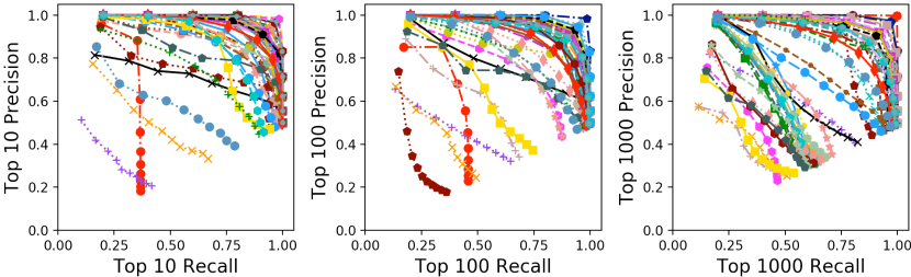
Figure 2: Precision versus recall for the top 10, top 100, and top 1000 ground edge-local triangle count truth heavy hitters of all SNAP graphs and all 5 synthetic kronecker graphs.

We examined the performance of the local $t$-neighborhood estimation algorithm (Algorithm 2) with prefix size of 8 on 10 moderately sized SNAP graphs up to $t=5$. Figure 1 displays the MRE of the returned local estimates. We find that the MRE matches our expectations informed by Theorem 1. In early passes, most of the neighborhoods are relatively small and so in practice the cardinality sketches give very precise estimates. As $t$ grows, the neighborhood balls grow to saturate the graph and so accordingly the estimation error grows until leveling off around the theoretical error guarantee.

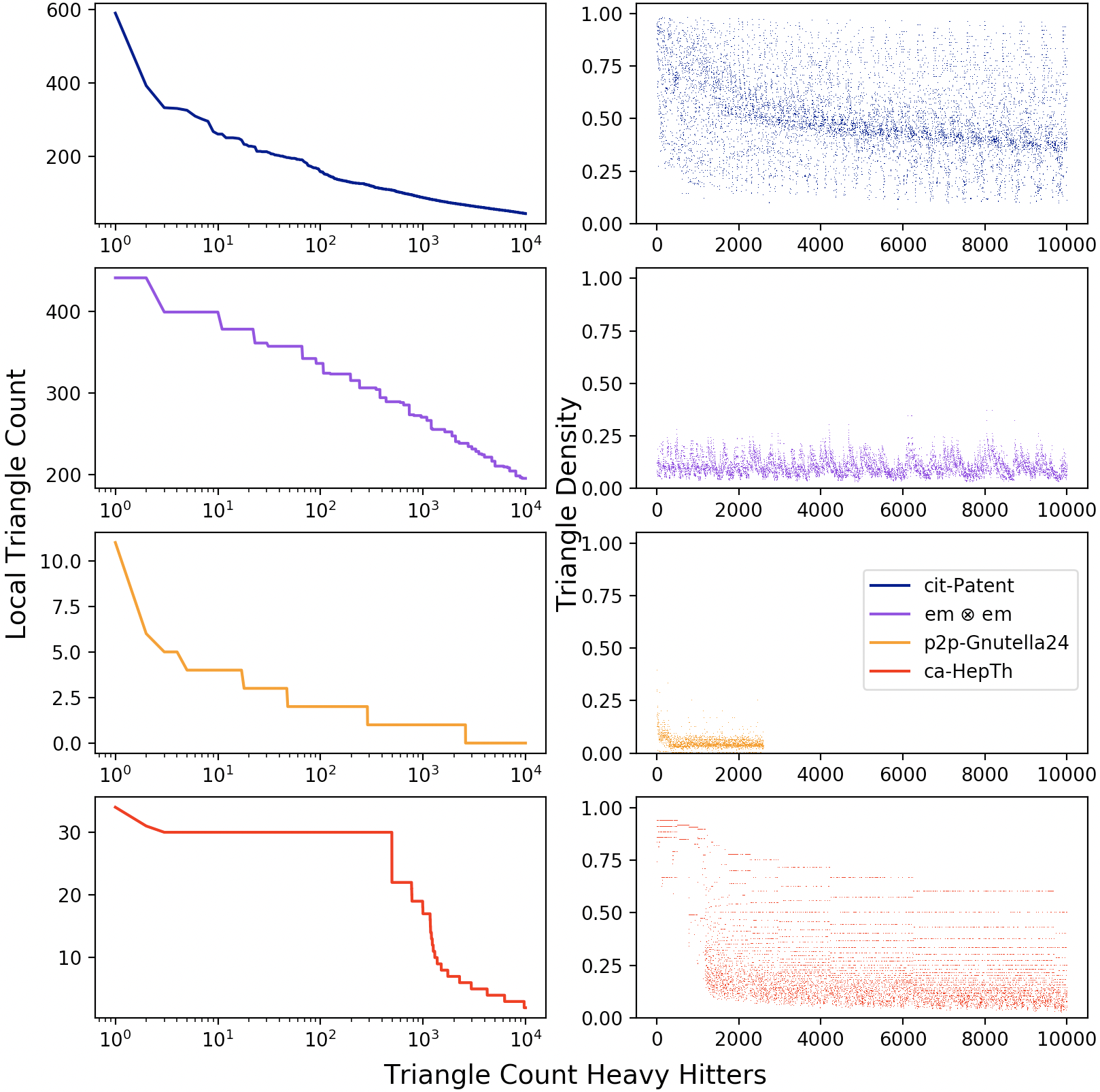
Figure 3: The triangle counts and triangle densities of the edge-local triangle count heavy hitters up to $10^{4}$ for four graphs.

We experimented with Algorithm 4 with a prefix size of 12, attempting to collect the top $k=10,100,1000$ heavy hitters $\mathcal{H}_{k}$ for all of the SNAP and Kronecker graphs. For each $k$, we ran the algorithm with $k^{\prime}$ ranging from $0.2*k$ up to $2*k$, producing $\widetilde{\mathcal{H}}_{k^{\prime}}$. We performed a similar analysis and found similar results for Algorithm 5, and omit them for space.

Treating $\widetilde{\mathcal{H}}_{k^{\prime}}$ as a one-class classifier of elements in $\mathcal{H}_{k}$, an edge $e\in\mathcal{E}$ is a true positive if $e\in\mathcal{H}_{k}\cap\widetilde{H}_{k^{\prime}}$, a false negative if $e\in\mathcal{H}_{k}\setminus\widetilde{\mathcal{H}}_{k^{\prime}}$, a false positive if $e\in\widetilde{\mathcal{H}}_{k^{\prime}}\setminus\mathcal{H}_{k}$, or a true negative if $e\not\in\mathcal{H}_{k}\cup\widetilde{\mathcal{H}}_{k^{\prime}}$.

We can report the quality of experiments in terms of its recall $\left(\frac{TP}{TP+FN}\right)$ versus its precision $\left(\frac{TP}{TP+FP}\right)$ for each setting of $k$ and $k^{\prime}$ in Figure 3. The precision versus recall tradeoff is a common metric in information retrieval, where the goal is to tune model parameters so as to force both the precision and recall as close to one as possible. Although these measures are known to exhibit bias, they are accepted as being reasonable for heavily uneven classification problems such as ours, where the class of interest is a small proportion of the samples (Boughorbel et al., 2017). Although most graphs show very good precision versus recall curves, there are a few notable outliers.

Figure 3 contrasts the edge-local triangle count distribution between a graph with good performance in Figure 2 and three with relatively poor performance. We find that triangle density, or the ratio of edge-local triangles versus the union of endpoint adjacency sets is a powerful determiner of performance. Triangle density corresponds with the Jaccard similarity of the edge’s endpoint neighbor sets, and for neighbor sets $A$ and $B$ is computed as $\frac{|A\cap B|}{|A\cup B|}$. In other words, again, relatively small intersections produce high error and uncertain heavy hitter recovery.

The cit-Patent graph exhibits good performance in Figure 2, and demonstrates a reasonable triangle count distribution as well as high triangle density throughout in Figure 3. The other three graphs demonstrate poor performance in Figure 2. The kronecker em $\otimes$ em graph exhibits an unusual number of ties in its triangle count distribution due to its construction, in addition to low triangle density among its heavy hitters. The P2P-Gnutella24 graph has very low triangle density, and a 3 or fewer triangles for the vast majority of its edges. The ca-HepTh graph exhibits an unusual triangle distribution, where a huge portion of its edges tie at 30 triangles. Consequently, even a perfect heavy hitter extraction procedure will fail on this graph. Notably, the two edges with the largest triangle counts are reliably returned.

Table 1: Scaling Graphs

graph	$|\mathcal{V}|$	$|\mathcal{E}|$	Type
patents	3,774,768	16,518,947	Citation
ye $\boldsymbol{\otimes}$ ye	5,574,320	88,338,632	Kronecker
or $\boldsymbol{\otimes}$ or	131,859,288	1,095,962,562	Kronecker
Twitter	41,652,224	1,201,045,942	S. N. (Kunegis, 2013)
WDC	3,563,602,788	128,736,914,864	Web

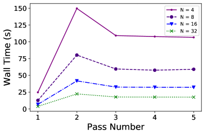
Figure 4: The time in seconds to perform local $t$-neighborhood size estimation up to $t=5$ for the or $\otimes$ or graph for nodes $N=4,8,16.32$.

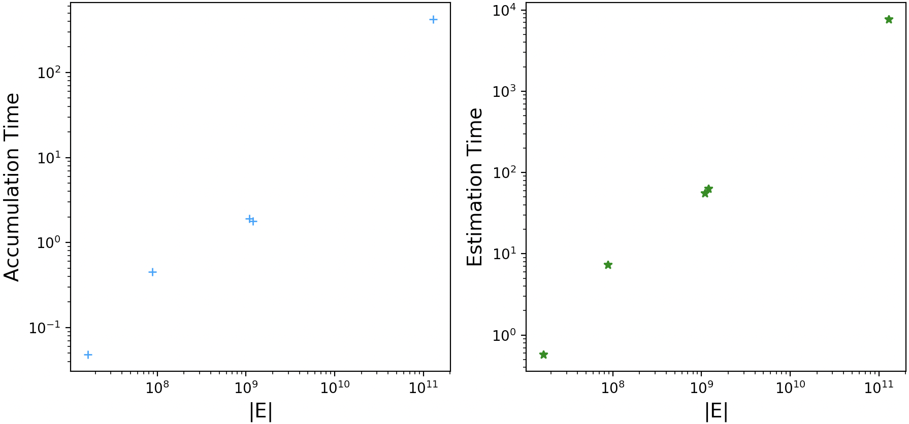
Figure 5: The time in seconds to accumulate and perform local triangle count estimation using $N=72$ compute nodes for all graphs listed in Table 1.

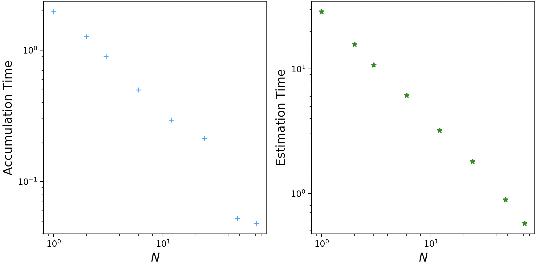
Figure 6: The time in seconds to accumulate and perform local triangle count estimation using $N=1$ up to $72$ for the citation-Patents graph.

We also examined the performance scaling of the algorithms as a function of data and computing resource sizes. For each experiment we used a prefix size of 8 and discounted the I/O time spent on reading data streams from files. Algorithms 4 and  5 exhibit near-identical time performance, and so we report only the later.

We ran Algorithm 2 for $t=5$ on the or $\otimes$ or Kronecker graph, varying the number of nodes from $N=4,8,16,32$. We note nice weak scaling behavior: as the computational resources double, the time roughly halves. In particular, pass 2 tends to take more time because of the sparsity settings in our implementations; merges are less efficient for sparse sketches. Once the sketches saturate, note that the time decreases significantly in later passes. One could implement DegreeSketch using only dense sketches to avoid this hump. If one only intends to perform local $t$=neighborhood estimation, omitting sparse sketches is a good idea as all sketches will eventually saturate as $t$ grows.

Similarly, Figure 6 measures the the time in seconds spent for Algorithms 1 and  5 on the cit-Patents graph, where $N$ varies from 1 up to 72. This weak scaling experiment demonstrates significant performance improvements on a fixed amount of work as resources increase.

It is difficult to demonstrate strong scaling using graph data, as graphs (especially realistic ones) do not scale smoothly like, say, linear algebra. We instead present a ”strong scaling” experiment on the 5 large graphs in Table 1. We found that subsequent passes of Algorithm 2 exhibited similar behavior to Algorithm 5, and so we only report results for the latter.

Figure 5 measures the the time in seconds spent accumulating DegreeSketch and performing the vertex-local estimation on each graph, plotted against the number of edges in each graph. We used $N=72$ compute nodes in each case. As promised, the wall time is linear in the number edges for both accumulation and estimation, showing good scaling with graph size on fixed resources. We found in experiments that the subsequent passes of Algorithm 2 experienced similar linear scaling.

It is worth noting that a competing state-of-the-art exact triangle counting algorithm required $N=256$ compute nodes to even load the largest WebDataCommons graph into distributed memory (Pearce, 2017).

6 Conclusions

We have herein demonstrated the efficacy of DegreeSketch to scalably and approximately answering queries on massive graphs. Although we have focused on estimating neighborhood sizes and counting triangles, DegreeSketch’s utility extends to more general queries that can be phrased as unions and possibly an intersection of adjacency sets. In particular, although we have focused on simple undirected graphs in this work, colored graphs are an interesting area of future work. A simple generalization to the work here presented allows us to estimate interesting queries of the form ”how many of $x$’s $t$-neighbors are both red and green?” or ”how many of $x$’s $t$-neighbors are not blue?” DegreeSketch’s demonstrated scalability coupled with its demonstrated performance should prove useful in applications where such queries are prevalent, such as motif counting.

7 Acknowledgments

This work was performed under the auspices of the U.S. Department of Energy by Lawrence Livermore National Laboratory under Contract DE-AC52-07NA27344 (LLNL-CONF-757958). Experiments were performed at the Livermore Computing Facility.

Appendix A Vertex-Local Variance Bound

The following theorem bounds the estimator error variance of Algorithm 5 in terms of the variances of the atomic edge-local estimates using the subadditivity of the standard deviation - i.e. if random variables $a$ and $b$ have finite variance, $\sqrt{\mathrm{Var}\left[a+b\right]}\leq\sqrt{\mathrm{Var}\left[a\right]}+\sqrt{\mathrm{Var}\left[b\right]}$:

Theorem 2.

Let $\widetilde{\mathcal{T}}(x)$ be the estimated output of Algorithm 5 for $x\in\mathcal{V}$, and let $\widetilde{\mathcal{T}}(xy)$ be the estimated edge triangle count for $xy\in\mathcal{E}$. Assume further that for each $xy$, we know a standard deviation bound $\eta_{xy}$ so that

$$\frac{\sqrt{\mathrm{Var}\left[\widetilde{\mathcal{T}}(xy)\right]}}{\mathcal{T}(xy)}\leq\eta_{xy}.$$ (20)

Furhermore, let $\eta_{*}=\max_{xy\in\mathcal{E}}\eta_{xy}$. Then, $\widetilde{\mathcal{T}}(x)$ has at most twice this maximum standard deviation. That is,

$$\frac{\sqrt{\mathrm{Var}\left[\widetilde{\mathcal{T}}(x)\right]}}{\mathcal{T}(x)}\leq 2\eta_{*}.$$

Proof.

$$\frac{\sqrt{\mathrm{Var}\left[\widetilde{\mathcal{T}}(x)\right]}}{\mathcal{T}(x)} =\frac{\sqrt{\mathrm{Var}\left[\sum\limits_{xy\in\mathcal{E}}\widetilde{\mathcal{T}}(xy)\right]}}{\mathcal{T}(x)}$$

$$\leq\frac{\sum\limits_{xy\in\mathcal{E}}\sqrt{\mathrm{Var}\left[\widetilde{\mathcal{T}}(xy)\right]}}{\mathcal{T}(x)}$$ subadditivity

$$\leq\frac{\sum\limits_{xy\in\mathcal{E}}\eta_{xy}\mathcal{T}(xy)}{\mathcal{T}(x)}$$ Equation (20)

$$\leq\frac{\eta_{*}\sum\limits_{xy\in\mathcal{E}}\mathcal{T}(xy)}{\mathcal{T}(x)}$$

$$=2\eta_{*}$$ Equation (5)

∎

Theorem 2 shows that if we can bound the error variance of the edge-local triangle count estimates produced using DegreeSketch, we can also bound the error variance of the vertex-local triangle count estimates produced by Algorithm 5. Unfortunately, we are unable to provide these bounds a priori, as they depend upon the sizes of all of the the sets and their intersections, which are an unknown function of the graph. However, if we are somehow promised that the triangle density of every edge is above a given threshold, we are able to produce analytic guarantees of the estimation error.

Appendix B Dominations and Small Intersections

We have noted that there are limitations to the sketch intersection estimation in Section 4.1. There appear to be two main sources of large estimation error in practice. Throughout we will borrow the parlance of Section 4.1.

The first source of error is the phenomenon where $\mathbf{r}^{(A)}_{i}>\mathbf{r}^{(B)}_{i}$ for all $i$ where $\mathbf{r}^{(B)}_{i}>0$, resulting in $\mathbf{c}^{(A),<}_{k}=\mathbf{c}^{(B),>}_{k}=0$ for all $k$ and $\mathbf{c}^{=}_{k}=0$ for all $k>0$. This generally only occurs when $|A|\gg|B|$ or $B\subseteq A$. We say that such an $A$ strictly dominates $B$. In this case, Equation (70) of (Ertl, 2017) can be rewritten as the sum of functions depending upon $\lambda_{a}$ and $\lambda_{b}+\lambda_{x}$. This means that the optimization relative to $\lambda_{a}$ does not depend upon $\lambda_{x}$ or $\lambda_{b}$. The optimization relative to $\lambda_{b}+\lambda_{x}$ is similarly independent of $\lambda_{a}$, and thus is tantamount to using the maximum likelihood estimator for $B$ independent of $A$. Consequently, $\lambda_{x}$ could be anything between 0 and $\widetilde{\lambda}_{(B)}$ without affecting the optimum joint likelihood, resulting in arbitrary estimates for the intersection.

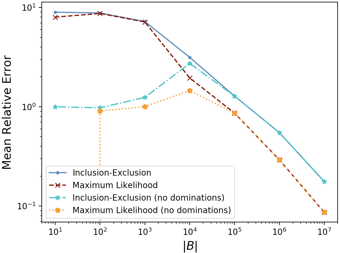
Figure 7: Mean relative intersection error as a function of $|B|$, where $|A\cap B|=\frac{|B|}{10}$.

We also consider the phenomenon where $\mathbf{r}^{(A)}_{i}\geq\mathbf{r}^{(B)}_{i}$ for all $i$, resulting in $\mathbf{c}^{(A),<}_{k}=\mathbf{c}^{(B),>}_{k}=0$ for all $k$. We say that such an $A$ dominates $B$. We are unable to make the same analytic statements about Equation (70), as the terms dependent upon $\mathbf{c}^{=}$ are not eliminated. Consequently, the optimum estimate for $\lambda_{a}$ depends upon $\lambda_{b}$ and $\lambda_{x}$. If $A$ dominates $B$, the count statistics given by Equation 19 are unable to distinguish whether $B$ is subset of $A$. Many and large nonzero values for $\mathbf{c}^{=}_{k}$ for large $k$ will bias the optimization towards larger intersections, whereas the converse is true if $\mathbf{c}^{=}_{k}$ is nonzero for only a few small values of $k$. If $|A|\gg|B|$, then the latter might occur whether $|A\cap B|$ is large or small. Furthermore, note that if $B\subseteq A$, then $A$ will (possibly strictly) dominate $B$.

If $A$ dominates $B$, then $S^{(A\cup B)}=S^{(A)}$. Ergo, the inclusion-exclusion estimator returns the estimated value of $B$. This estimate is dubious, given that we have no evidence that the sets $A$ and $B$ hold any elements in common. This is especially true if $|A|\gg|B|$. Hence, both the naïve and maximum likelihood estimators may suffer from bias when a domination event occurs. Figure 7 plots the mean relative error as one of the sets decreases, with a fixed relative intersection size. As $|B|$ gets smaller, the likelihood of a domination increases. At $|B|=10^{4}$ dominations occur in $6.6\%$ of cases, at $|B|=10^{3}$ dominations occur in $76.9\%$ of cases, at $|B|=10^{2}$ dominations occur in $97.5\%$ of cases, and at $|B|=10$ dominations occur in $99.8\%$ of cases. In particular in the two cases where $|B|=10$ and $|A\cap B|=1$ and a domination does not occur, the maximum likelihood estimator returns exactly 1. So for a fixed intersection size relative to $|B|$, both the inclusion-exclusion and maximum likelihood estimators return more reasonable estimates when dominations do not occur. However, there is no known reliable method to avoid them in practice.

Consequently, it might be safest to disregard dominations in practice, as failing to do so is theoretically unsound and likely to produce high and arbitrary error. However, this poses a problem for many graph applications, as one will frequently have to compare the sketches of high degree vertices with those of comparatively low degree to find their joint triangle count.

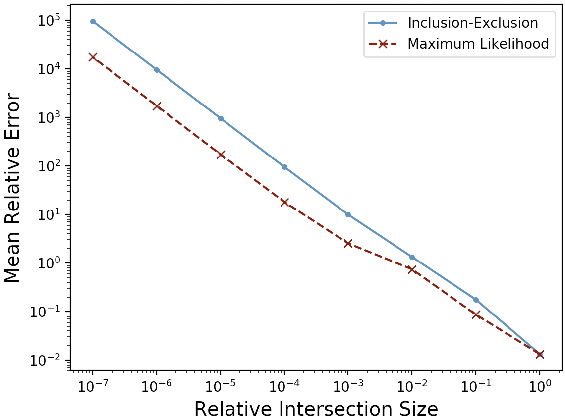
Figure 8: HLL inclusion-exclusion and maximum likelihood intersection estimator performance where $|A|=|B|=10^{7}$ and $|A\cap B|$ varies from $1$ up to $|B|$.

We have also noted the problem of small intersections. As discussed above, the maximum likelihood intersection estimate is proportional to the number (and size) of the nonzero $\mathbf{c}^{=}_{k}$ for $k>0$, where larger $k$ biases the estimate toward larger intersections. If the ground truth intersection is small relative to $|A|$ and $|B|$, however, Equation (70) will exhibit high variance.

Figure 8 compares the performance of the inclusion-exclusion estimator to the maximum likelihood estimator for a prefix size of 12. Here the set sizes are kept constant at $10^{7}$ Note that the mean relative error grows quite large as the relative interection size decreases, although the maximum likelihood estimator consistently outperforms the inclusion-exclusion estimator by roughly an order of magnitude.

Appendix C Kronecker Graph Construction

Nonstochastic Kronecker graphs (Weichsel, 1962) have adjacency matrices $C$ that are Kronecker products $C=C_{1}\otimes C_{2}$, where the factors are also adjacency matrices. This type of synthetic graph is attractive for testing graph analytics at massive scale (Leskovec et al., 2010; Kepner et al., 2018), as ground truth solution is often cheaply computable. For such graphs, global triangle count and triangle counts at edges are computed via Kronecker formulas (Sanders et al., 2018): for a graph with $m$ edges, the worst-case cost of computing global triangle counts is sublinear, $O\left(m^{\frac{3}{4}}\right)$, whereas the cost of computing the full set of edge-local counts is $O\left(m\right)$.

Here, we build $C=C_{1}\otimes C_{2}$ from identical factors, $C_{1}=C_{2}$, that come from a small set of graphs with $m$ up to $10^{5}$ from the University of Florida sparse matrix collection (polbooks, celegans, geom, yeast (Davis & Hu, 2011)). All graphs were forced to be undirected, unweighted, and without self loops. We compute the number of triangles at each edge for $C_{1}$ and use the Kronecker formula in (Sanders et al., 2018) to get the respective quantities for $C$. Summing over the edges and dividing by 3 gives the global triangle count for $C$.

References

- Ahmed et al. (2017) Nesreen K Ahmed, Nick Duffield, Theodore L Willke, and Ryan A Rossi. On sampling from massive graph streams. Proceedings of the VLDB Endowment, 10(11):1430–1441, 2017.
- Alon et al. (1999) Noga Alon, Yossi Matias, and Mario Szegedy. The space complexity of approximating the frequency moments. Journal of Computer and System Sciences, 58:137–147, 1999.
- Arifuzzaman et al. (2013) Shaikh Arifuzzaman, Maleq Khan, and Madhav Marathe. Patric: A parallel algorithm for counting triangles in massive networks. In Proceedings of the 22nd ACM international conference on Information & Knowledge Management, pp. 529–538. ACM, 2013.
- Bar-Yossef et al. (2002) Ziv Bar-Yossef, TS Jayram, Ravi Kumar, D Sivakumar, and Luca Trevisan. Counting distinct elements in a data stream. In International Workshop on Randomization and Approximation Techniques in Computer Science, pp. 1–10. Springer, 2002.
- Becchetti et al. (2008) Luca Becchetti, Paolo Boldi, Carlos Castillo, and Aristides Gionis. Efficient semi-streaming algorithms for local triangle counting in massive graphs. In Proceedings of the 14th ACM SIGKDD international conference on Knowledge discovery and data mining, pp. 16–24. ACM, 2008.
- Becchetti et al. (2010) Luca Becchetti, Paolo Boldi, Carlos Castillo, and Aristides Gionis. Efficient algorithms for large-scale local triangle counting. ACM Transactions on Knowledge Discovery from Data (TKDD), 4(3):13, 2010.
- Berry et al. (2011) Jonathan W Berry, Bruce Hendrickson, Randall A LaViolette, and Cynthia A Phillips. Tolerating the community detection resolution limit with edge weighting. Physical Review E, 83(5):056119, 2011.
- Boldi et al. (2011) Paolo Boldi, Marco Rosa, and Sebastiano Vigna. Hyperanf: Approximating the neighbourhood function of very large graphs on a budget. In Proceedings of the 20th international conference on World wide web, pp. 625–634. ACM, 2011.
- Boughorbel et al. (2017) Sabri Boughorbel, Fethi Jarray, and Mohammed El-Anbari. Optimal classifier for imbalanced data using matthews correlation coefficient metric. PloS one, 12(6):e0177678, 2017.
- Chu & Cheng (2011) Shumo Chu and James Cheng. Triangle listing in massive networks and its applications. In Proceedings of the 17th ACM SIGKDD international conference on Knowledge discovery and data mining, pp. 672–680. ACM, 2011.
- Cohen (2008) Jonathan Cohen. Trusses: Cohesive subgraphs for social network analysis. National Security Agency Technical Report, 16, 2008.
- Cohen et al. (2017) Reuven Cohen, Liran Katzir, and Aviv Yehezkel. A minimal variance estimator for the cardinality of big data set intersection. In Proceedings of the 23rd ACM SIGKDD International Conference on Knowledge Discovery and Data Mining, pp. 95–103. ACM, 2017.
- Collet (2014) Yann Collet. xxHash. https://github.com/Cyan4973/xxHash, 2014. Accessed: 2018-12-20.
- Davis & Hu (2011) Timothy A Davis and Yifan Hu. The university of florida sparse matrix collection. ACM Transactions on Mathematical Software (TOMS), 38(1):1, 2011.
- Durand & Flajolet (2003) Marianne Durand and Philippe Flajolet. Loglog counting of large cardinalities. In European Symposium on Algorithms, pp. 605–617. Springer, 2003.
- Ertl (2017) Otmar Ertl. New cardinality estimation algorithms for hyperloglog sketches. arXiv preprint arXiv:1702.01284, 2017.
- Estan et al. (2003) Cristian Estan, George Varghese, and Mike Fisk. Bitmap algorithms for counting active flows on high speed links. In Proceedings of the 3rd ACM SIGCOMM conference on Internet measurement, pp. 153–166. ACM, 2003.
- Flajolet & Martin (1985) Philippe Flajolet and G Nigel Martin. Probabilistic counting algorithms for data base applications. Journal of computer and system sciences, 31(2):182–209, 1985.
- Flajolet et al. (2007) Philippe Flajolet, Éric Fusy, Olivier Gandouet, and Frédéric Meunier. Hyperloglog: the analysis of a near-optimal cardinality estimation algorithm. In Discrete Mathematics and Theoretical Computer Science, pp. 137–156. Discrete Mathematics and Theoretical Computer Science, 2007.
- Gupta et al. (2013) Pankaj Gupta, Ashish Goel, Jimmy Lin, Aneesh Sharma, Dong Wang, and Reza Zadeh. Wtf: The who to follow service at twitter. In Proceedings of the 22nd international conference on World Wide Web, pp. 505–514. ACM, 2013.
- Heule et al. (2013) Stefan Heule, Marc Nunkesser, and Alexander Hall. Hyperloglog in practice: algorithmic engineering of a state of the art cardinality estimation algorithm. In Proceedings of the 16th International Conference on Extending Database Technology, pp. 683–692. ACM, 2013.
- Jha et al. (2013) Madhav Jha, Comandur Seshadhri, and Ali Pinar. A space efficient streaming algorithm for triangle counting using the birthday paradox. In Proceedings of the 19th ACM SIGKDD international conference on Knowledge discovery and data mining, pp. 589–597. ACM, 2013.
- Kane et al. (2010) Daniel M Kane, Jelani Nelson, and David P Woodruff. An optimal algorithm for the distinct elements problem. In Proceedings of the twenty-ninth ACM SIGMOD-SIGACT-SIGART symposium on Principles of database systems, pp. 41–52. ACM, 2010.
- Kepner et al. (2018) Jeremy Kepner, Siddharth Samsi, William Arcand, David Bestor, Bill Bergeron, Tim Davis, Vijay Gadepally, Michael Houle, Matthew Hubbell, Hayden Jananthan, et al. Design, generation, and validation of extreme scale power-law graphs. arXiv preprint arXiv:1803.01281, 2018.
- Kunegis (2013) Jérôme Kunegis. Konect: the koblenz network collection. In Proceedings of the 22nd International Conference on World Wide Web, pp. 1343–1350. ACM, 2013.
- Leskovec & Krevl (2014) Jure Leskovec and Andrej Krevl. SNAP Datasets: Stanford large network dataset collection. http://snap.stanford.edu/data, June 2014.
- Leskovec et al. (2010) Jure Leskovec, Deepayan Chakrabarti, Jon Kleinberg, Christos Faloutsos, and Zoubin Ghahramani. Kronecker graphs: An approach to modeling networks. Journal of Machine Learning Research, 11(Feb):985–1042, 2010.
- Lim & Kang (2015) Yongsub Lim and U Kang. Mascot: Memory-efficient and accurate sampling for counting local triangles in graph streams. In Proceedings of the 21th ACM SIGKDD International Conference on Knowledge Discovery and Data Mining, pp. 685–694. ACM, 2015.
- Milo et al. (2002) Ron Milo, Shai Shen-Orr, Shalev Itzkovitz, Nadav Kashtan, Dmitri Chklovskii, and Uri Alon. Network motifs: simple building blocks of complex networks. Science, 298(5594):824–827, 2002.
- Myers et al. (2014) Seth A Myers, Aneesh Sharma, Pankaj Gupta, and Jimmy Lin. Information network or social network?: the structure of the twitter follow graph. In Proceedings of the 23rd International Conference on World Wide Web, pp. 493–498. ACM, 2014.
- Palmer et al. (2002) Christopher R Palmer, Phillip B Gibbons, and Christos Faloutsos. Anf: A fast and scalable tool for data mining in massive graphs. In Proceedings of the eighth ACM SIGKDD international conference on Knowledge discovery and data mining, pp. 81–90. ACM, 2002.
- Pearce (2017) Roger Pearce. Triangle counting for scale-free graphs at scale in distributed memory. In High Performance Extreme Computing Conference (HPEC), 2017 IEEE, pp. 1–4. IEEE, 2017.
- Priest et al. (2019) Benjamin Priest, Trevor Steil, Roger Pearce, and Geoff Sanders. You’ve Got Mail: Building missing asynchronous communication primitives. In Proceedings of the 2019 International Conference on Supercomputing, pp. 8. ACM, 2019.
- Qin et al. (2016) Jason Qin, Denys Kim, and Yumei Tung. Loglog-beta and more: A new algorithm for cardinality estimation based on loglog counting. arXiv preprint arXiv:1612.02284, 2016.
- Sanders et al. (2018) Geoffrey Sanders, Roger Pearce, Timothy La Fond, and Jeremy Kepner. On large-scale graph generation with validation of diverse triangle statistics at edges and vertices. arXiv preprint arXiv:1803.09021, 2018.
- Shin et al. (2018a) Kijung Shin, Mohammad Hammoud, Euiwoong Lee, Jinoh Oh, and Christos Faloutsos. Tri-Fly: Distributed estimation of global and local triangle counts in graph streams. In Pacific-Asia Conference on Knowledge Discovery and Data Mining, pp. 651–663. Springer, 2018a.
- Shin et al. (2018b) Kijung Shin, Euiwoong Lee, Jinoh Oh, Mohammad Hammoud, and Christos Faloutsos. Dislr: Distributed sampling with limited redundancy for triangle counting in graph streams. arXiv preprint arXiv:1802.04249, 2018b.
- Stefani et al. (2017) Lorenzo De Stefani, Alessandro Epasto, Matteo Riondato, and Eli Upfal. Trièst: Counting local and global triangles in fully dynamic streams with fixed memory size. ACM Transactions on Knowledge Discovery from Data (TKDD), 11(4):43, 2017.
- Suri & Vassilvitskii (2011) Siddharth Suri and Sergei Vassilvitskii. Counting triangles and the curse of the last reducer. In Proceedings of the 20th international conference on World wide web, pp. 607–614. ACM, 2011.
- Ting (2016) Daniel Ting. Towards optimal cardinality estimation of unions and intersections with sketches. In Proceedings of the 22nd ACM SIGKDD International Conference on Knowledge Discovery and Data Mining, pp. 1195–1204. ACM, 2016.
- Tsourakakis (2008) Charalampos E Tsourakakis. Fast counting of triangles in large real networks without counting: Algorithms and laws. In Data Mining, 2008. ICDM’08. Eighth IEEE International Conference on, pp. 608–617. IEEE, 2008.
- Tsourakakis et al. (2009) Charalampos E Tsourakakis, U Kang, Gary L Miller, and Christos Faloutsos. Doulion: counting triangles in massive graphs with a coin. In Proceedings of the 15th ACM SIGKDD international conference on Knowledge discovery and data mining, pp. 837–846. ACM, 2009.
- Wang et al. (2010) Nan Wang, Jingbo Zhang, Kian-Lee Tan, and Anthony KH Tung. On triangulation-based dense neighborhood graph discovery. Proceedings of the VLDB Endowment, 4(2):58–68, 2010.
- Weichsel (1962) Paul M Weichsel. The kronecker product of graphs. Proceedings of the American mathematical society, 13(1):47–52, 1962.
- Wolf et al. (2017) Michael M Wolf, Mehmet Deveci, Jonathan W Berry, Simon D Hammond, and Sivasankaran Rajamanickam. Fast linear algebra-based triangle counting with kokkoskernels. In High Performance Extreme Computing Conference (HPEC), 2017 IEEE, pp. 1–7. IEEE, 2017.