Bayesian Interpolants as Explanations for Neural Inferences
Abstract
The notion of Craig interpolant, used as a form of explanation in automated reasoning, is adapted from logical inference to statistical inference and used to explain inferences made by neural networks. The method produces explanations that are at the same time concise, understandable and precise.
1 Introduction
Statistical machine learning models, most notably deep neural networks, have recently proven capable of accomplishing a remarkable variety of tasks, such as image classification, speech recognition, and visual question answering, with a degree of precision formerly only achievable by humans. There has been increasing concern, however, about the opacity of these models. That is, while the models may produce accurate predictions, they do not produce explanations of these predictions that can be understood and validated by humans. As noted by O’Neil [12], this opacity can have substantially negative social consequences. From a purely technical point of view, it creates an obstacle to improving models and methods.
This paper addresses the question of what it means for a model to produce a meaningful explanation of a statistical prediction or inference. We take as our starting point a notion of explanation used in automated reasoning. In Boolean satisfiability (SAT) solving [1] and model checking [4], one typically reasons from particular cases to the general case. For example, in SAT solving, we may consider a partial assignment of truth values to Boolean variables. In model checking, we might consider a particular control path of a program. To generalize from a particular case, we need an explanation of why a property holds in that case. An explanation has two key characteristics: it must be a simple proof of the property, and it must be expressed in a form that can be generalized. The notion of simplicity is a bias: it prevents over-fitting the explanation to the particular case. The formal or syntactic requirement depends on the kind of generalization we wish to perform.
In automated reasoning, the explanation is often expressed as a Craig interpolant. Given a logical premise that implies a conclusion , an interpolant for this implication is an intermediate predicate , such that:
-
•
implies ,
-
•
implies , and
-
•
is expressed only using variables that are in common to and .
Notice that the first two requirements are semantic, while the last is syntactic. This is crucial to the interpretation of interpolants as explanations. From an intuitive point of view, for to explain a fact to , it must speak ’s language, abstracting away concepts irrelevant to . It is this abstraction that affords generalization. The notion of interpolation as explanation was proposed from a philosophical point of view by Hintikka and Halonen [7]. From a practical point of view, McMillan showed that interpolation could be used to derive facts about intermediate states in specific program executions. These facts could be generalized to an inductive invariant proving the general case [11]. In retrospect, the conflict clauses [16] used in SAT solvers can also be seen as interpolants. In these applications, the key properties of an interpolant are that it should be simple, in order to avoid over-fitting, and it should use the right vocabulary, in order to abstract away irrelevant concepts.
How, then can we transfer this notion of explanation of a logical inference to some notion of explanation of a statistical inference? In this paper, we will explore the idea of using a kind of naive Bayesian “proof”. An inference in this proof will be of the form where is a desired degree of certainty. We will maintain the notion of finding an intermediate fact in the proof that uses the “right” vocabulary. In the statistical setting, however, our premise and conclusion need not have any variables in common. This is because the premise and conclusion are connected by an underlying probability distribution. Thus, instead of using the common vocabulary, we will simply choose some set of variables that we consider to be causally intermediate between premise and conclusion . We then define a (naïve) Bayesian interpolant to be a predicate over the intermediate variables such that and . That is, if we observe , then is probably true, and if we observe , then is probably true. This is a “naïve” proof because it implies that , but only under the unwarranted assumption that and are independent given .
We will explore the application of Bayesian interpolants as explanations for inferences made by artificial neural networks (ANN’s). In this case, the premise is an input presented to the network, the conclusion is the prediction made by the network, and the vocabulary represents (typically) the activation of the network at some hidden layer. We will observe that, despite possibly unjustified assumptions, interpolation can produce explanations that are both understandable to humans, and remarkably precise.
The paper is organized as follows. In section 2, we formalize the notion of Bayesian interpolant. In section 3, we define inference of interpolants as a multi-objective optimization problem, and introduce a simple framework for learning interpolants from data. In section 4, we apply the approach to a convolutional neural model for the MNIST digit recognition problem, interpreting the results and comparing them to existing methods.
2 Bayesian interpolants
Let be a set of observables. Each observable has a range, denoted . An observation is a map that takes each observable to an element of its range. Now let be a probability space, where is a set of observations, is a -algebra over (the measurable sets) and is the probability measure, assigning probabilities to sets in .
Example 1
We are given an ANN that classifies images of hand-written digits with layers, the first being the input layer and the last the output layer. The observable is the activation of the -th unit in the -th layer, while observable is the digit prediction. We have and . The observables in layers are functionally determined by the input layer. That is, for and any observation , we have and .
Let be a language of formulas. The vocabulary of a formula , denoted , is a subset of the observables . If is an observation and is a formula, we write to indicate that is a model of (that is, is true in ). We write for the set of models of . We require that the truth value of a formula depends only on its vocabulary, that is, if two observations and agree on the observables in , then if and only if . We further require that is closed under conjunction. That is, if and are formulas, then so is , and moreover:
-
•
-
•
iff and .
Finally, we require that, for all , the models of form a measurable set, that is, . In the sequel, we will abuse notation by writing simply for when the intention is clear. For example, we will write for the probability that is true, which is .
Example 2
For the ANN example, let be the set of finite conjunctions of atomic predicates of the form , and , where is an observable and is a numeric constant, for example .
Definition 1
Suppose that and are formulas in , is a set of observables, and is a probability in . We say that a -interpolant is formula such that and:
| (1) | ||||
| (2) |
provided the above conditional probabilities are well-defined.
Example 3
We wish to explain why the ANN classifies a particular image as digit 7. In this case, our premise is (stating that the input image is ) and our conclusion is . We seek a fact about layer 2 that explains the prediction 7. Thus, we let . After a search, we discover a -interpolant: . This fact about a pair of layer 2 units holds for image and predicts that the network will output 7 with precision 0.95. We consider this fact an explanation because it is simple and expressed over variables that are causally intermediate between input and output.
An additional figure of merit for an interpolant is its recall, which we define as . The recall is the fraction of positive occurrences of the conclusion that are predicted by the interpolant. The recall gives us a measure of how likely the interpolant is to be applicable in cases where the premise is false. While high recall is not required for an explanation, we will observe that a minimum value is needed for statistical significance.
Definition 2
A -interpolant is a -interpolant that also satisfies:
| (3) |
3 Learning interpolants
In the case of learned models, the underlying probability space is hypothetical. In place of the distribution, we are given a data set that is presumed to be an i.i.d. sample from the distribution. Thus, we cannot solve eqs. 1 to 3 exactly, but instead must treat these constraints as hypotheses to be tested. In this section, we will introduce a machine learning approach to discover interpolants. The method uses a training data set for hypothesis formation and an independent test data set for confirmation.
As might be expected, there is a trade-off among precision, recall and simplicity. For example, we may increase simplicity at the expense of recall, or recall at the expense of precision. The learning approach has hyper-parameters to control this trade-off. Moreover, recall, training set size and variance are related. That is, if the number of samples satisfying is low, then the confidence in the statistical test of eq. 2 is correspondingly low. Thus we will find that generalization is likely to fail, in the sense that precision on the test set is lost.
A dataset is a finite indexed family of observations. A dataset induces a probability measure distribution such that is the frequency of satisfaction of in the dataset, that is:
| (4) |
We will write for the sub-family .
Interpolation can be seen as a multi-objective constrained optimization problem. That is, given a dataset , we would like to solve eqs. 1 to 3 for while maximizing , and minimizing the syntactic complexity of .
It is tempting to try to apply standard learning approaches, e.g., gradient boosted trees [6] or random forests [2], to solve this optimization problem. However, while these methods allow a degree of trade-off between recall and precision, they are not well-suited to explore the Pareto front. We cannot, for example, use them to solve for the most precise classifier of a certain complexity having a fixed recall.
Instead, we introduce here a technique that solves the multi-objective optimization problem for atomic predicates by exhaustive search. It then uses a simple boosting technique that conjoins new predicates in order to improve precision at the expense of recall, until a target precision is reached. Thus, we attempt to minimize complexity and maximize recall, for a fixed precision,
3.1 Atomic Bayesian interpolants
An atomic predicate is one without any logical connectives, such as conjunction or if-then-else. As an example, in decision tree learning, the atomic predicates label the decision nodes and are usually of the form or , where is an observable and is a constant. We will call these upper (respectively lower) bound predicates. For these predicates, it is practical to learn optimal interpolants by exhaustive search.
Given fixed values of and , we can find bound predicates that satisfy eq. 1 and eq. 3 by computing fractiles. We define the upper fractile , where is a probability, an observable, and a formula, as the least such that . Similarly, the lower fractile is the greatest such that . For , we can compute fractiles in time, where is the number of data points, by simply sorting with respect to .
Figure 1 shows a procedure AtomicInterp that computes an atomic interpolant for given values of and , optimizing the precision . The set contains, for each observable , the strongest lower bound predicate satisfying eq. 1 and eq. 3 (thus, the one with minimal recall). The set contains the corresponding upper bound predicates. Among these, the procedure chooses the one with the maximal precision. Minimizing recall (subject to the constraints) is not guaranteed to find the interpolant with maximal precision. However, it is a good heuristic, since in general precision increases with decreasing recall.
| procedure AtomicInterp(,,,,,) | ||
| requires and | ||
| with : | ||
| return |
Example 4
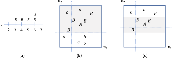
Suppose , , and is distributed as in fig. 2(a). The relevant fractiles are , , , . This gives us and . We have while . Thus, we return .
3.2 Conjunctive Bayesian interpolants
A single atomic predicate is unlikely to provide sufficient precision to act as a useful explanation. The procedure of fig. 3 boosts the precision of the interpolant by conjoining predicates until a precision goal is reached. At each step, the recall constraint is reduced by a factor to allow the interpolant to be strengthened. Moreover, we keep only the data points satisfying the current interpolant , to focus on eliminating the remaining false positives. The procedure terminates when the precision goal is achieved, or the complexity of the interpolant reaches a maximum . As a measure of the complexity of , we can use the number of bound predicates, which we denote .
| procedure ConjInterp(,,,,,,,) | ||
| requires and | ||
| while and : | ||
| return |
Example 5
Suppose , , and , and suppose the dataset is distributed as in fig. 2(b). The dotted lines show the -th fractiles. The interpolant at the first step is the shaded region. It has a precision of and a recall of . Figure 2(b) shows the result of boosting the precision by conjoining a predicate. We consider only the points satisfying . The resulting precision is , and the recall is . Since the precision is greater than , the algorithm terminates.
If both and are close to one, then interpolation becomes essentially transfer learning. That is, we are attempting to learn a new predictor as a function of a representation learned by the ANN. In this case, however, we would necessarily sacrifice simplicity, and thus explanatory power. By relaxing the requirement for recall, we gain in simplicity, and are thus able to form useful explanations. For this purpose, and should lie in a “sweet spot”, where both complexity and variance are low.
The procedure described above is just an example of a method for learning interpolants. Conjunctions of bound predicates are a natural choice, since they are easy to compute and to understand, and they allow us to boost precision by sacrificing recall. Other sorts of atomic predicates are possible, however, for example, linear constraints. One could also generalize conjunctions to, say, decision trees. An important difference between interpolation and common learning problems is that, in seeking an explanation for a particular inference, high recall is not required but some lower bound on recall is needed. This means that existing learning approaches may need to be modified to learn interpolants. Nonetheless, one could attempt to explore the space of interpolants by using existing loss-based approaches and simply scaling down the loss associated with false negatives. If this is effective, it would open up a wide range of possible approaches.
4 Example: MNIST digit recognition task
In this section, we experiment with using Bayesian interpolants as explanations for inferences made by ANN’s. As an example, we use the MNIST hand-written digit database [10]. This consists of labeled -pixel gray-scale images of hand-written digits, and has been widely used as a benchmark for both learning and explanation methods.
The ANN model we use has five layers: 1) the input layer, 2) a linear convolutional layer with kernel and 28 channels ( units in total), 3) a max-pooling layer ( units in total), 4) a fully-connected layer of 128 units with RELU activation, and 5) a fully-connected output layer of 10 units with soft-max activation. This model is implemented in the Keras framework [8] and trained on the 60,000-image MNIST training sample using the Adam optimizer with sparse categorical cross-entropy loss function. It achieved 98.2% accuracy over the 10,000-image MNIST test set.
We begin by computing interpolants at layer 3, the max-pooling layer, because this layer has 1/4 of the units of the convolutional layer, but is still localizable in the image (each unit corresponds to region of pixels). For each experiment, we choose an input image whose output category (i.e., the output unit with highest activation) is . We wish to produce an explanation for this inference, so our premise is (which we take as an abbreviation for ) and our conclusion is . To ensure that , we must include image in the dataset.
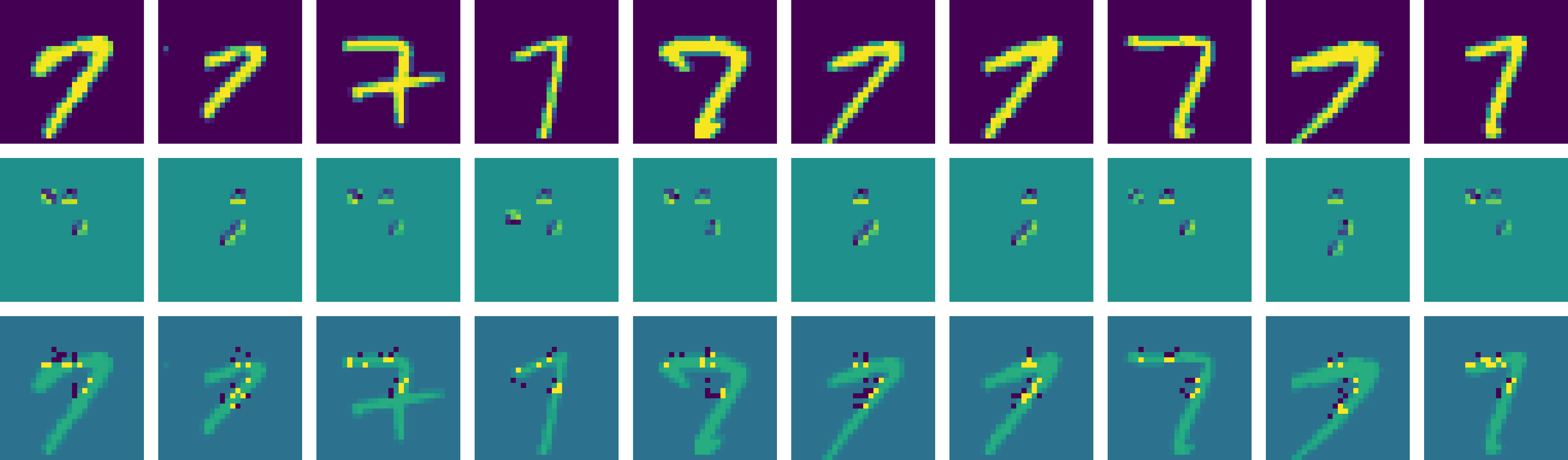
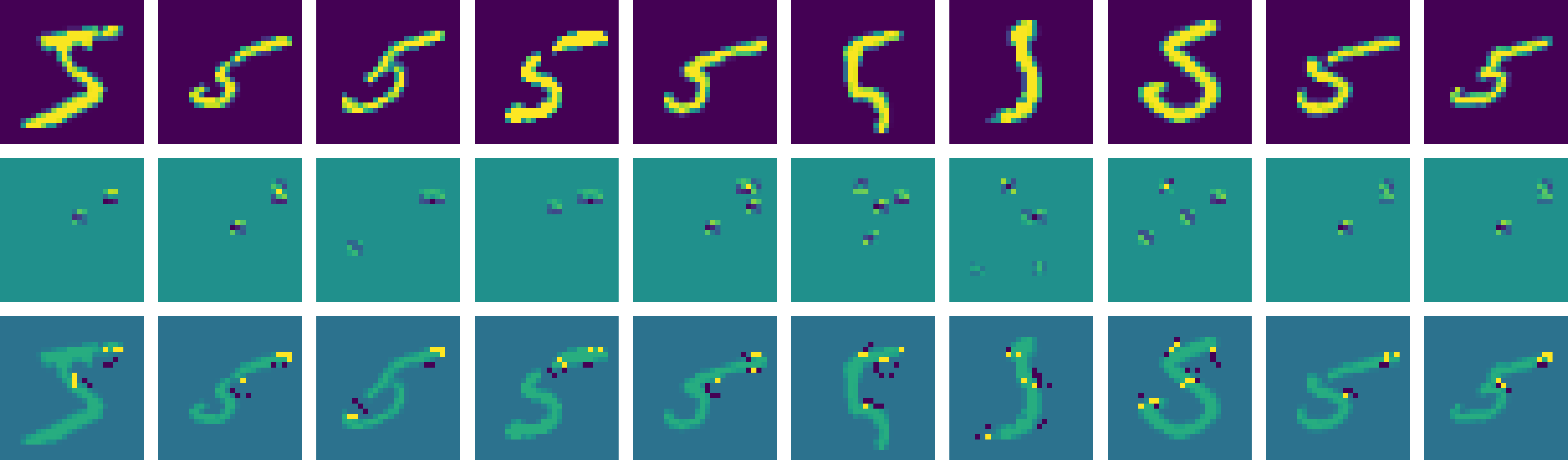
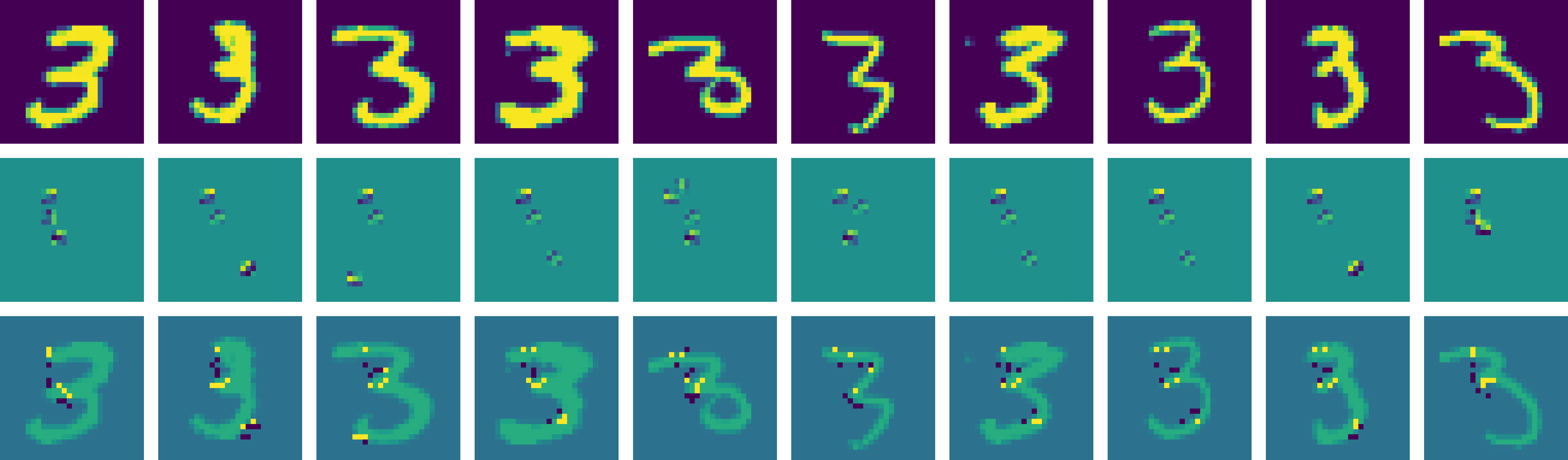
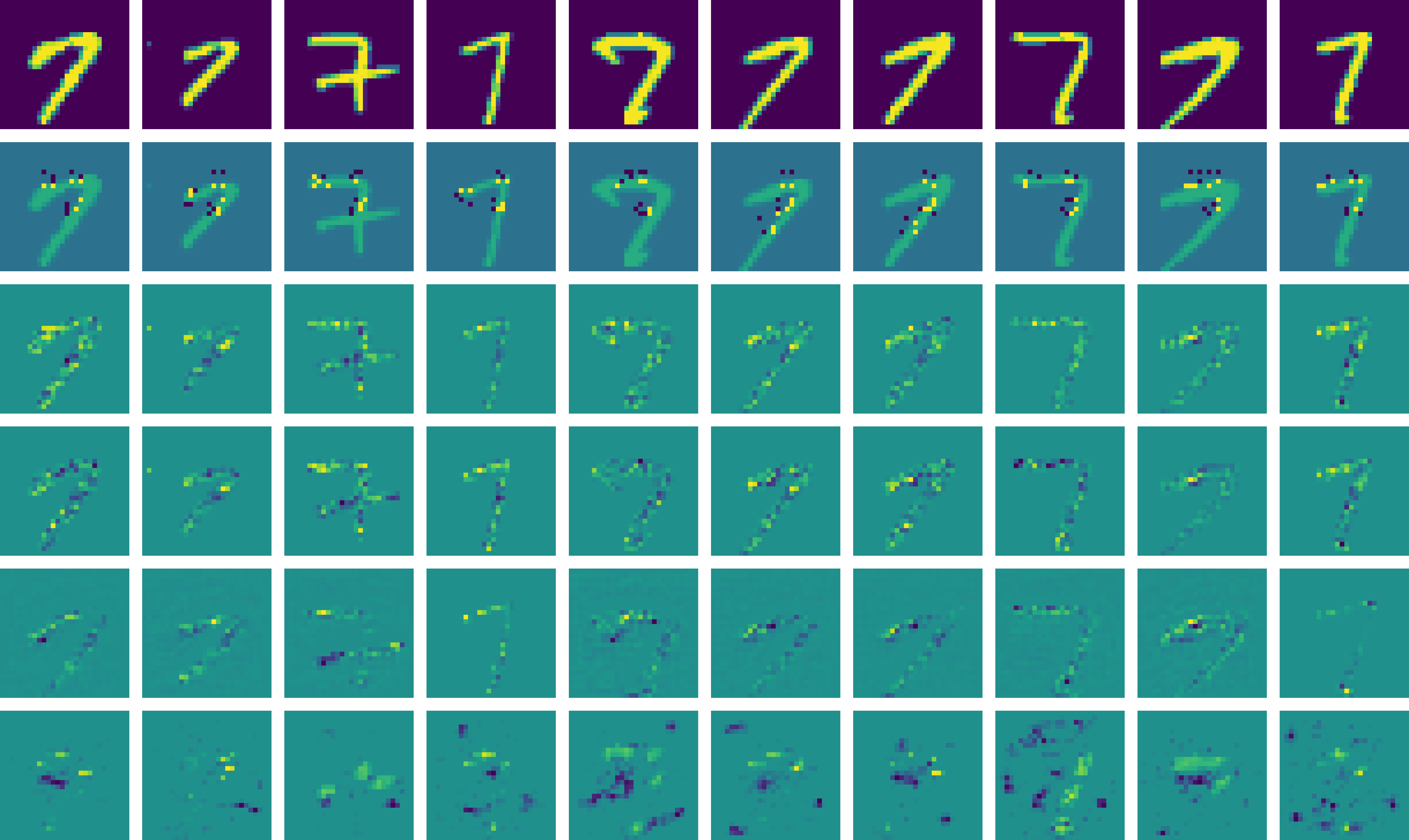
We compute interpolants using procedure ConjInterp where is the first 20,000 images in the training set. Figure 4 shows interpolants computed for the first 10 images in the training set classified by the model as digits 7, 5 and 3, with , and (the digits were chosen in advance of seeing the data, to avoid cherry-picking). For each case, the input images are shown in the top row. The middle row images are a superposition of the kernels of the units used in the interpolant. Due to pooling, each kernel shown is actually applied over a region of pixels. For the digit seven, we can see that the typical number of units used in the interpolant is three out of 4,732, while for the more complex figure three, typically 3–4 units are needed. The average complexity of the interpolants for digit seven is 3.2 conjuncts, the average precision is 0.982, and the average recall is 0.123. That is, just three out of 4,732 units are needed to predict the outcome with 98% precision.
In fig. 5, we see plots of the average precision, recall and interpolant complexity obtained, as a function of the hyper-parameters and , keeping fixed at . Complexity is measured as the number of atomic predicates. The figures are averaged over 1000 input images, selected as the first 100 images classified by the ANN as digit , for . To ensure that the interpolants generalize, precision and recall are calculated over the test dataset, not the training dataset. As we increase (the lower bound on the recall of atomic interpolants) the recall of the interpolant increases. At the same time, the average number of conjuncts in the interpolant increases, reflecting the fact that more boosting steps are needed to achieve the target precision for a higher recall. Notably, precision on the test set increases slightly with recall (note that the precision scale in the plots has a very narrow range). This may seem counter-intuitive, since the opposite relationship typically holds. Notice, however, that with lower recall, the interpolant is true on fewer samples in the training set. Optimizing the precision over a small set of samples can lead to over-fitting of the interpolant, and thus to reduced precision on the test set. Therefore, while we do not require high recall for purposes of explanation, we need to set some lower bound on recall in order for the interpolants to generalize well. The peaks in precision may be caused by the fact that precision on the training set drops off slightly with increasing recall and complexity. Thus there is a “sweet spot” balancing training precision and generalization.
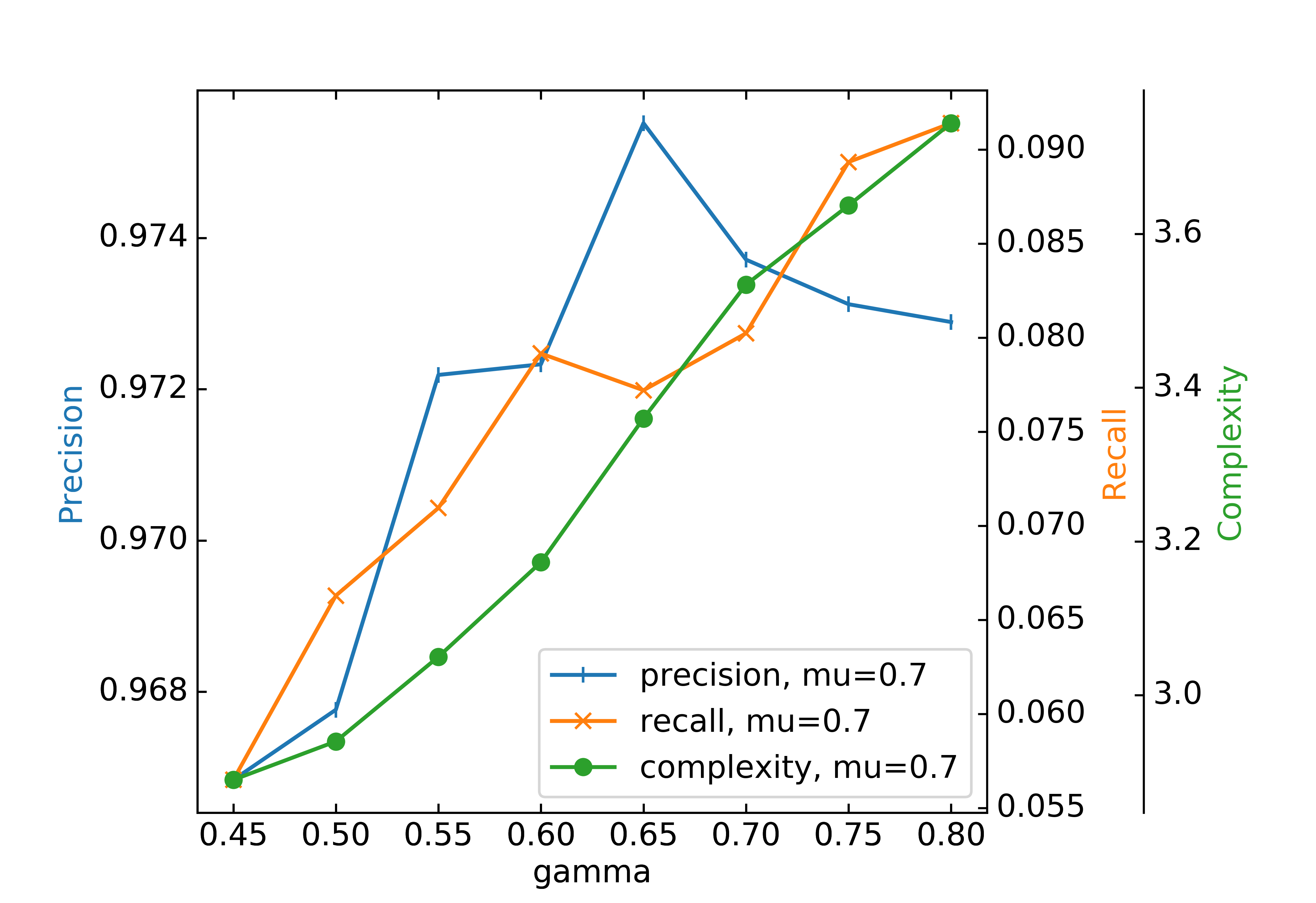
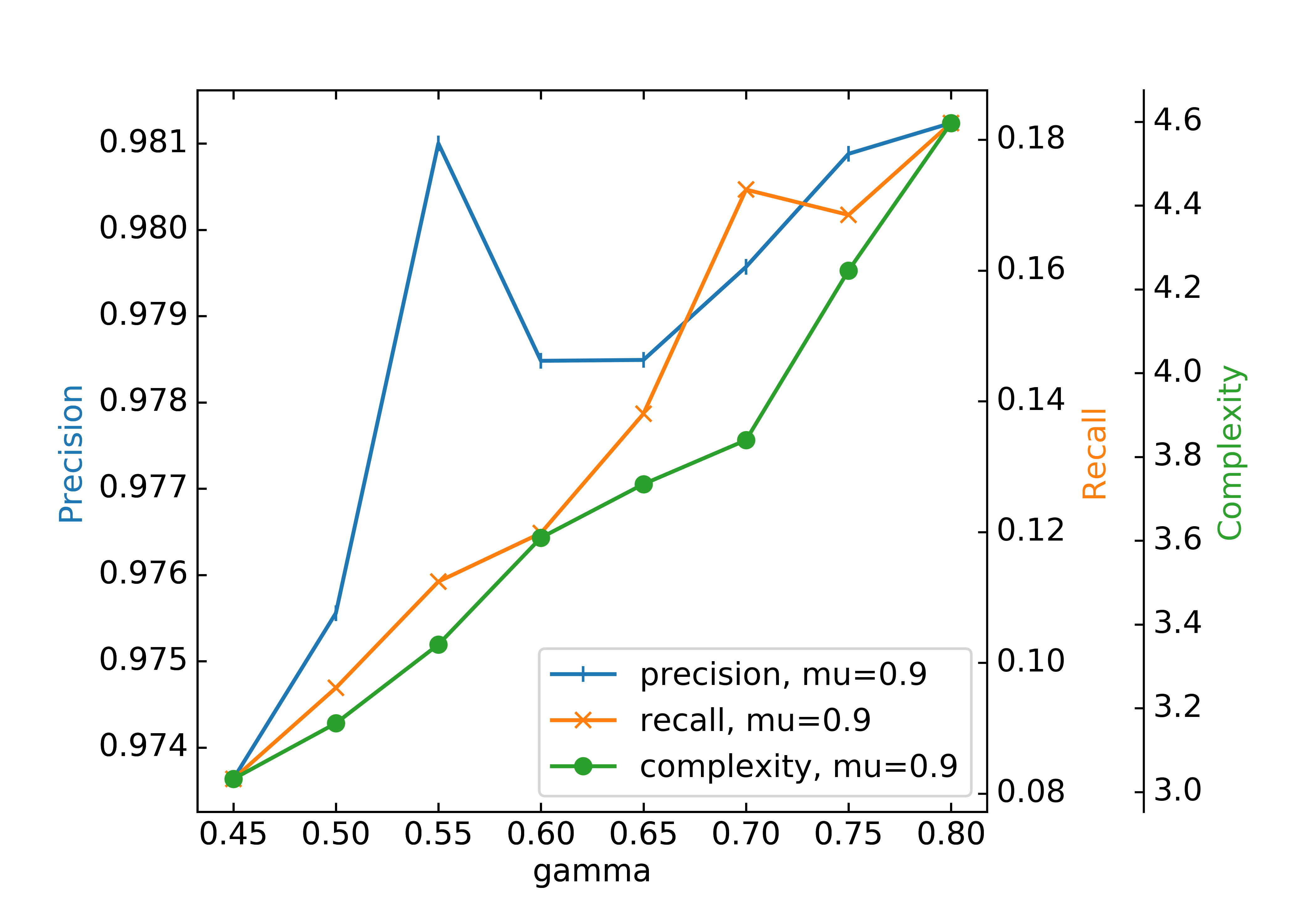
Figure 5 clearly shows a trade-off of simplicity of the interpolant vs. precision. To be a useful explanation, the interpolant must be both simple and highly predictive, thus we must make this trade-off carefully. In the MNIST application, a sweet spot occurs at around 3.3 conjuncts, with precision around , which we can achieve with parameter values and .
4.1 Sequence interpolants
While the layer-3 interpolants give a sense of the general regions of the image that are important for predicting the output, the kernels themselves are difficult to interpret. For example, in some cases, complex kernels that appear to be edge or line detectors are actually being used in dark regions of the image. This is interesting, as the ANN may be opportunistically using features for purposes for which they are not optimally tuned.
To explain the activation of these units by a particular image, we can apply interpolation a second time. That is, we learn an interpolant at the input layer (layer 1) that predicts the layer-3 interpolant. In effect, we are constructing a naïve Bayesian proof in three steps: the image predicts a fact about the input layer, which in turn predicts a fact about an internal layer, which in turn predicts the output. Such a multi-stage proof could be called a sequence interpolant.
For the layer-1 interpolant we can take advantage of the convolutional structure of the network to introduce a regularization. That is, we know that each convolutional unit is causally dependent on only a small region of the input pixels. Thus, for each conjunct of the layer 3 interpolant , we learn a layer-1 interpolant over just the patch of the input image on which the corresponding layer-3 unit depends. Our layer-1 interpolant is the conjunction . In this way, we exploit our knowledge that certain observables are relevant in order to introduce bias, and thus hopefully better generalization than we would obtain by directly learning a layer-1 interpolant that predicts the output. We will see that this strategy can be quite effective.
In fig. 4, the third row of images for each digit shows a representation of the atomic predicts in the layer-1 interpolant thus obtained, with the input image faintly superposed. Like the layer-3 interpolants, the layer-1 interpolants are computed with , and . A dark magenta pixel indicates an upper bound predicate, while a bright yellow pixel indicates a lower bound predicate. The light green pixels are not part of the interpolant. These interpolants are much easier to interpret than the kernels of the layer-3 interpolant. For example, in the case of digit seven, it is clear that the most important predictive feature is typically the corner in the upper right of the seven. Above an to the left of the two strokes, a dark region is required. For digit five, the top horizontal stroke is most prominent (with exceptions for two oddly formed digits). Notice that the interpolant for the oddly shaped figure five in column 7 is still consistent with a more typically shaped five. For digit three, the three horizontal segments are most prominently used. To get a sense of how strong these interpolants are as predictions, try to draw a realistic figure of a different digit (centered in the image) that passes through the bright points without touching the dark points.
How precise are these interpolants in predicting the ANN’s output? Each interpolant predicates the corresponding atomic predicate with precision of about , and the conjunction of the in turn predicts the outcome with about the same precision. Using the naïve assumption that these probabilities are independent, we would estimate predicts the output with a precision of about or . To evaluate the actual obtained precision, we used as a test set the 40,000 held-out images from the training set. We need a large test set because the average recall of is only 0.005. Even with large test set, 51% of the 1000 interpolants were true on zero images in the test set, thus the precision could not be estimated, as the denominator was zero. On the remaining 49% of interpolants, the average precision was 0.996. The cumulative precision of all predictions made by the interpolants was also 0.996 (that is, over all 1000 interpolants, the false positive rate was 0.004).
This anomalously high precision requires explanation. Previously, we observed that low recall led to reduced precision, due to over-fitting to a small sample. In this case, however, there is no over-fitting because the are learned independently and over different features of the input space. Like a random forest, this is an example of stochastic discrimination [9]. Each has by itself a good precision and moderate recall over the test set in predicting . By forming the conjunction, we in effect boost this precision over both the training and test sets, at the expense of recall. Notice that, unlike a random forest, the weak predictors in our interpolant have been selected to predict features of another model that explain its output in a particular case. This is very different from random selection (i.e., bagging) but has a similar effect of improving generalization.
What is still puzzling, however, is that actually predicts the output more strongly than . One way to interpret this is that, because of correlations in the input space, predicts stronger bounds at layer 3 than those represented by the conjuncts of . Thus, because the output depends causally on layer 3, it is more strongly predicted by than by . This implies that we could reasonably trade some precision for simplicity in by reducing the parameter .
It is remarkable to observe that the small fraction of pixels used in the interpolants of fig. 4 (on average 12.4 out of 784) can predict the ANN output with such high precision. One way to look at this is that we obtained a combination of simplicity and generality by using the causal structure of the ANN as a regularizer.
We also note that the interpolants are not expensive to compute. The average time to compute both interpolants for the MNIST model is 2.8s on an 8-core, 3.6GHz Intel Xeon processor, using the numpy library in Python.
4.2 Comparison to other explanation techniques
Many techniques have been explored for producing human-understandable explanations of neural inferences, especially for image classification tasks. Many use the same gradient computation that is used for training the network to identify input units of high sensitivity, relative to a baseline input. Figure 6 compares of the layer-1 interpolants to the results of three gradient-based methods: Integrated Gradients [17], DeepLift [15], and Guided Grad-CAM [14] (all as implemented in the Captum tool [3]) as well as the Contrastive Explanation Method (CEM) which is based on adversarial generation [5], as implemented by its authors [13].
Results are shown for the first 10 images categorized as digit seven by the network. In the gradient-based methods, bright yellow pixels are attributed as positively influencing the digit seven output, while dark magenta pixels are negatively influencing. Because the all-zero image is used as the baseline, these methods do not indicate relevance of background pixels. For CEM, the bright pixels represent a subset of the image’s foreground pixels that is classified as seven. The dark pixels represent background pixels that, if activated, would cause the image to be classified as not seven.
We observe that the Integrated Gradients and DeepLift methods do not localize the inference. That is, almost all foreground pixels are assigned positive or negative influence. The Grad-CAM method does somewhat localize some images. All of the methods attribute negative influence to many foreground pixels. None offers any clear explanation of the inference. On the other hand, the interpolants are specific, and they point to a key feature in the recognition of a digit seven: the sharp angle in the upper right. Moreover, the interpolants show the influence of background pixels in recognizing the angle, while the gradient methods do not consider the background. Most importantly, the interpolants are predictive: they predict the inference with an average precision of 99.6% over the test set. The gradient-based explanations only give a general notion that certain regions of the image may be more relevant than others.
The CEM method does succeed in some cases in localizing the explanation (columns 1–3,6,7). However, in these cases the explanation is not precise, as it is possible to draw a figure other that seven that is consistent with the images (for example a two in cols. 1,2,6,7, or a four in col. 3). On the other hand, the explanations that appear to be precise are not simple. Thus the method does not make a good trade-off between simplicity and precision.
5 Conclusion
In automated reasoning, we often seek explanations in terms of simple proofs that can be generalized. This idea is used to learn from failures in SAT solving, to refine abstractions in model checking, and to generalize proofs about loop-free programs into inductive proofs about looping programs. In this paper, we have explored a statistical analog of this concept of explanation, with the purpose of giving explanations of inferences made by statistical models such as ANN’s. The form of the explanation is a Bayesian interpolant: a chain of statistical inferences leading from a premise to a conclusion. The structure of this chain is informed by the causal structure of the model, which acts as a regularizer or bias, allowing us to construct a simple and yet highly precise explanation.
It is important to understand that a Bayesian interpolant is a statistical explanation, not a causal explanation. In principle, it is possible that the observables that are used to express an interpolant are not even logically connected to the output, but are merely correlated with it. If our concern is in gaining confidence in the model’s inference, and not in how the model arrives at it, then this is not an issue. However, interpolants do tell us something about how the ANN works. The existence of very simple interpolants with high precision tells us the representations used by the ANN are highly redundant. As in automated deduction, interpolants may point to important features in the ANN, or they may suggest more predictive features than the ones actually used. They might also allow us to compress the network or compile it into a more efficiently computable form.
Because Bayesian explanations are quantitative predictions, they may provide a way to address the problem of fairness in statistical models. That is, suppose we have a model that is trained on a dataset that reflects bias on the part of human decision makers, or societal bias that impacts outcomes. How can we determine whether a given inference made by the model is fair or rational? If the inference comes with a Bayesian explanation that depends only on variables that we consider to be a rational basis for decisions, and yet at the same time is highly predictive of the outcome, then we may consider the inference to be acceptable. On the other hand, if the explanation depends on variables that we consider irrelevant or irrational, then we may reject it. Moreover, a simple and predictive explanation may act as a guide in the case of an undesired outcome, and reduce the opacity of the model to those affected by its inferences.
References
- [1] Armin Biere, Marijn Heule, Hans van Maaren, and Toby Walsh, editors. Handbook of Satisfiability, volume 185 of Frontiers in Artificial Intelligence and Applications. IOS Press, 2009.
- [2] Leo Breiman. Random forests. Mach. Learn., 45(1):5–32, 2001.
- [3] Captum. Captum: Model interpretability for pytorch. https://captum.ai/, 2020. retrieved 2020-04-03.
- [4] Edmund M. Clarke, Thomas A. Henzinger, Helmut Veith, and Roderick Bloem, editors. Handbook of Model Checking. Springer, 2018.
- [5] Amit Dhurandhar, Pin-Yu Chen, Ronny Luss, Chun-Chen Tu, Pai-Shun Ting, Karthikeyan Shanmugam, and Payel Das. Explanations based on the missing: Towards contrastive explanations with pertinent negatives. In Samy Bengio, Hanna M. Wallach, Hugo Larochelle, Kristen Grauman, Nicolò Cesa-Bianchi, and Roman Garnett, editors, Advances in Neural Information Processing Systems 31: Annual Conference on Neural Information Processing Systems 2018, NeurIPS 2018, 3-8 December 2018, Montréal, Canada, pages 590–601, 2018.
- [6] Jerome H. Friedman. Greedy function approximation: A gradient boosting machine. Ann. Statist., 29(5):1189–1232, 10 2001.
- [7] Jaakko Hintikka and Ilpo Halonen. Interpolation as explanation. Philosophy of Science, 66:S414–S423, 1999.
- [8] Keras. Keras documentation. https://keras.io/, 2020. retrieved 2020-04-03.
- [9] E. M. Kleinberg. Stochastic discrimination. Ann. Math. Artif. Intell., 1:207–239, 1990.
- [10] Yann LeCun, Léon Bottou, Yoshua Bengio, and Patrick Haffner. Gradient-based learning applied to document recognition. Proceedings of the IEEE, 86(11):2278–2323, December 1998.
- [11] Kenneth L. McMillan. Interpolation and sat-based model checking. In Warren A. Hunt Jr. and Fabio Somenzi, editors, Computer Aided Verification, 15th International Conference, CAV 2003, Boulder, CO, USA, July 8-12, 2003, Proceedings, volume 2725 of Lecture Notes in Computer Science, pages 1–13. Springer, 2003.
- [12] Cathy O’Neil. Weapons of Math Destruction: How Big Data Increases Inequality and Threatens Democracy. Crown, 2016. First edition.
- [13] Github repository. Contrastive-explanation-method. https://github.com/IBM/Contrastive-Explanation-Method.git, 2020. retrieved 2020-04-03.
- [14] Ramprasaath R. Selvaraju, Michael Cogswell, Abhishek Das, Ramakrishna Vedantam, Devi Parikh, and Dhruv Batra. Grad-cam: Visual explanations from deep networks via gradient-based localization. In IEEE International Conference on Computer Vision, ICCV 2017, Venice, Italy, October 22-29, 2017, pages 618–626. IEEE Computer Society, 2017.
- [15] Avanti Shrikumar, Peyton Greenside, and Anshul Kundaje. Learning important features through propagating activation differences. CoRR, abs/1704.02685, 2017.
- [16] João P. Marques Silva and Karem A. Sakallah. GRASP: A search algorithm for propositional satisfiability. IEEE Trans. Computers, 48(5):506–521, 1999.
- [17] Mukund Sundararajan, Ankur Taly, and Qiqi Yan. Axiomatic attribution for deep networks. In Doina Precup and Yee Whye Teh, editors, Proceedings of the 34th International Conference on Machine Learning, ICML 2017, Sydney, NSW, Australia, 6-11 August 2017, volume 70 of Proceedings of Machine Learning Research, pages 3319–3328. PMLR, 2017.