Quantum Approximate Optimization of Non-Planar Graph Problems
on a Planar Superconducting Processor
Abstract
We demonstrate the application of the Google Sycamore superconducting qubit quantum processor to combinatorial optimization problems with the quantum approximate optimization algorithm (QAOA). Like past QAOA experiments, we study performance for problems defined on the (planar) connectivity graph of our hardware; however, we also apply the QAOA to the Sherrington-Kirkpatrick model and MaxCut, both high dimensional graph problems for which the QAOA requires significant compilation. Experimental scans of the QAOA energy landscape show good agreement with theory across even the largest instances studied (23 qubits) and we are able to perform variational optimization successfully. For problems defined on our hardware graph we obtain an approximation ratio that is independent of problem size and observe, for the first time, that performance increases with circuit depth. For problems requiring compilation, performance decreases with problem size but still provides an advantage over random guessing for circuits involving several thousand gates. This behavior highlights the challenge of using near-term quantum computers to optimize problems on graphs differing from hardware connectivity. As these graphs are more representative of real world instances, our results advocate for more emphasis on such problems in the developing tradition of using the QAOA as a holistic, device-level benchmark of quantum processors.
I Introduction
The Google Sycamore superconducting qubit platform has been used to demonstrate computational capabilities surpassing those of classical supercomputers for certain sampling tasks Arute et al. (2019). However, it remains to be seen whether such processors will be able to achieve a similar computational advantage for problems of practical interest. Along with quantum chemistry Aspuru-Guzik et al. (2005); O’Malley et al. (2016), machine learning Biamonte et al. (2016), and simulation of physical systems Lloyd (1996), discrete optimization has been widely anticipated as a promising area of application for quantum computers.
Beginning with a focus on quantum annealing Kadowaki and Nishimori (1998) and adiabatic quantum computing Farhi et al. (2001), the possibility of quantum enhanced optimization has driven much interest in quantum technologies over the years. This is because faster optimization could prove transformative for diverse areas such as logistics, finance, machine learning, and more. Such discrete optimization problems can be expressed as the minimization of a quadratic function of binary variables Lucas (2014); Barahona (1982), and one can visualize these cost functions as graphs with binary variables as nodes and (weighted) edges connecting bits whose (weighted) products sum to the total cost function value. For most industrially-relevant problems, these graphs are non-planar and many ancilla would be required to embed them in (quasi-)planar graphs matching the qubit connectivity of most hardware platforms Choi (2008). This limits the applicability of scalable architectures for quantum annealing Denchev et al. (2016) and corresponds to increased circuit complexity in digital quantum algorithms for optimization such as QAOA.
The quantum approximate optimization algorithm (QAOA) is the most studied gate model approach for optimization using near-term devices Farhi et al. (2014a). While the prospects for achieving quantum advantage with QAOA remain unclear, QAOA prescribes a simple paradigm for optimization which makes it amenable to both analytical results and implementation on current processors Farhi et al. (2014b); Biswas et al. (2017); Wecker et al. (2016); Farhi and Harrow (2016); Jiang et al. (2017); Wang et al. (2018); Hadfield et al. (2017); Lloyd (2018); Farhi et al. (2019). For these reasons, QAOA has also become popular as a system-level benchmark of quantum hardware. This work builds on prior experimental demonstrations of QAOA on superconducting qubits Otterbach et al. (2017); Willsch et al. (2019); Abrams et al. (2019); Bengtsson et al. (2019), ion traps Pagano et al. (2019), and photonics systems Qiang et al. (2018). We compare results from these past experiments in Appendix B.
We are able to experimentally resolve, for the first time, increased performance with greater QAOA depth and apply QAOA to cost functions on graphs that deviate significantly from our hardware connectivity. Owing to the low error rates of the Sycamore platform, the trade-off between the theoretical increase in quality of solutions with increasing QAOA depth and additional noise is apparent for hardware-native problems. We also apply the algorithm to non-native graph problems with their necessary compilation overhead and study the scaling of solution quality and problem size. Our results reveal that the performance of QAOA is qualitatively different when applied to hardware native graphs versus more complex graphs, highlighting the challenge of scaling QAOA to problems of industrial importance.
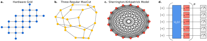
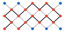
For this study, we used a “Sycamore” quantum processor which consists of a two-dimensional array of 54 transmon qubits Arute et al. (2019). Each qubit is tunably coupled to four nearest neighbors in a rectangular lattice. In this case, all device calibration was fully automated and data was collected using a cloud interface to the platform programmed using Cirq The Cirq Developers (2020). Our experiment was restricted to 23 physical qubits of the larger Sycamore device, arranged in a topology depicted in Figure 1a.
The combinatorial optimization problems we study in this work are defined through a cost function with a corresponding quantum operator given by
| (1) |
where is a classical bitstring, denotes the Pauli operator on qubit and the correspond to scalar weights with values . Because these clauses act on at most two qubits we are able to associate a graph with a given problem instance; if , there is an edge between and in the graph. We will study three families of problem graphs depicted in Figure 1.
The shallowest depth version of QAOA consists of the application of two unitary operators. At higher depths the same two unitaries are sequentially reapplied but with different parameters. We denote the number of repeated application of this pair of unitaries as , giving parameters. The first unitary prescribed by QAOA is
| (2) |
which depends on the parameter and applies a phase to pairs of bits according to the problem-specific cost function. The second operation is the driver unitary
| (3) |
where denotes the Pauli operator acting on qubit . This unitary drives transitions between bitstrings within the superposition state. These operators can be implemented by sequentially evolving under each term of the cost function, as suggested by Eq. (2) and Eq. (3).
For depth and qubits we prepare the state parameterized by and
| (4) |
where is the symmetric superposition of all computational basis states. The application of the QAOA circuit to this initial state is depicted in Figure 1d. For a given , we can find parameters to minimize the expectation value of the cost
| (5) |
For comparison among problem instances, we divide by , which is negative for all problems we study, so we are in fact maximizing .
II Compilation and Problem Families

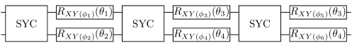
We approach compilation as two distinct steps: routing and gate synthesis. The need for routing arises when simulating for a cost function defined on a graph that is not a subgraph of our planar hardware connectivity. To simulate such we perform layers of swap gates (forming a swap network) which permute qubits such that all edges in the problem graph correspond to an edge in the hardware graph at least once, at which point the corresponding cost function terms can be implemented. An example of such a swap network is depicted in Figure 2a.
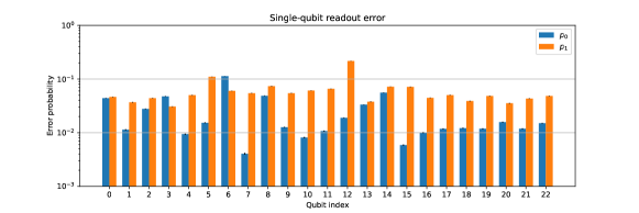
The final compilation step, gate synthesis, involves decomposing arbitrary 1- and 2-qubit interactions into physical gates supported by the device (see, e.g. Figure 2b). The physical gates used in this experiment are arbitrary single-qubit rotations and a two-qubit entangling gate native to the Sycamore hardware which we refer to as the syc gate and define in Figure 2c. Through multiple applications of this gate and single-qubit rotations, we are able to realize arbitrary entangling gates. Compilation details can be found in Appendix A. The average two-qubit gate fidelities on this device were 99.4% as measured by cross entropy benchmarking Arute et al. (2019) and average readout fidelity was 95.9% per qubit. We now discuss compilation for the three families of optimization problems studied in this work.
Hardware Grid Problems. Swap networks are not required when the problem graph matches the connectivity of our hardware; this is the main reason for studying such problems despite results showing that problems on such graphs are efficient to solve on average Barahona (1982); Rønnow et al. (2014). We generated random instances of hardware grid problems by sampling to be for edges in the device topology (and zero otherwise). Gates are scheduled so that the degree-four interaction graph can be implemented in four rounds of two-qubit gates by cycling through the interactions to the left, right, top and bottom of each interior qubit. Each two-qubit interaction can be synthesized with two layers of hardware-native syc gates interleaved with -dependent single-qubit rotations. In total, each application of the problem unitary is effected with eight total layers of syc gates.
Sherrington-Kirkpatrick (SK) Model. A canonical example of a frustrated spin glass is the Sherrington-Kirkpatrick model Sherrington and Kirkpatrick (1975). It is defined on the complete graph with randomly chosen to be . For large , optimal parameters are independent of the instance Farhi et al. (2019). The SK model is the most challenging model to implement owing to its fully-connected interaction graph. Optimal routing can be performed using the linear swap networks discussed in Ref. Hirata et al. (2011) and depicted in Figure 2. This requires layers of the composite interaction, each of which can be synthesized from three syc gates with interleaved -dependent single-qubit rotations. Thus, one application of the problem unitary can be effected in layers of syc gates.
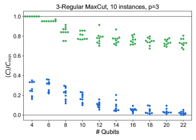
MaxCut on 3-Regular Graphs. MaxCut is a widely studied problem, and there is a polynomial-time algorithm due to Goemans and Williamson (1995) which guarantees a certain approximation ratio for all graphs, and it is an open question whether QAOA can efficiently achieve this or beat it Bravyi et al. (2019). Unlike the previous two problem families, all edge weights are set to , and we sample random 3-regular graphs to generate various instances. The connectivity of the problem Hamiltonian’s graph differs for each instance. While one could use the fully-connected swap network to route these circuits, this is wasteful. Instead, we used the routing functionality from the compiler to heuristically insert swap operations which move logical assignments to be adjacent Cowtan et al. (2019). These compiled circuits are of roughly equal depth to those from a fully-connected swap network, but the number of two qubit operations is roughly quadratically reduced.
III Energy Landscapes and Optimization
QAOA is a variational quantum algorithm where circuit parameters are optimized using a classical optimizer, but function evaluations are executed on a quantum processor Wecker et al. (2016); Yang et al. (2017); McClean et al. (2018). First, one repeatedly constructs the state with fixed parameters and samples bitstrings to estimate . On our superconducting qubit platform we can sample roughly five thousand bitstrings per second. A classical “outer-loop” optimizer can then suggest new parameters to decrease the observed expectation value. Note that we normalize by the cost function’s true minimum, so we are in fact maximizing ( is negative and hence, minimizing corresponds to maximizing ).
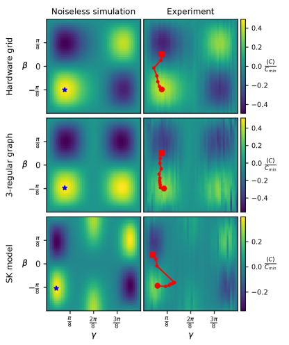
For , we can visualize the cost function landscape as a function of the parameters in a three-dimensional plot (where we drop the subscripts and label the axes and ). The presence of features like hills and valleys in the landscape gives confidence that a classical optimization can be effective. Comparison of simulated and empirical landscapes is a common qualitative diagnostic for the performance of experiments Qiang et al. (2018); Pagano et al. (2019); Willsch et al. (2019); Abrams et al. (2019); Bengtsson et al. (2019). For classical optimization to be successful the quantum computer must provide accurate estimates of . Otherwise, noise can overwhelm any signal making it difficult for a classical optimizer to improve the parameter estimates. Issues such as decoherence, crosstalk, and systematic errors manifest as differences (e.g., damping or warping) from the ideal landscape.
Figure 3 contains simulated theoretical and experimental landscapes for selected instances of the three problem families evaluated on a grid of and parameters with a resolution of 50 points along each linear axis. Each expectation value was estimated using 50,000 circuit repetitions with efficient post-processing to compensate for readout bias (see Appendix C). The hardware grid problem shows clear features at the maximum size of our study, . For the other two problems performance degrades with increasing and so we show data at for the 3-regular graph problem and for the SK model. We highlight the correspondence between experimental and theoretical landscapes for problems of large size and complexity. Prior experimental demonstrations have presented landscapes for a maximum of on a hardware-native interaction graph Pagano et al. (2019) and a maximum of for fully-connected problems like the SK model Abrams et al. (2019).
In Figure 3, we also overlay a trace of the classical optimizer’s path through parameter space as a red line. We used a classical optimizer called Model Gradient Descent (MGD) which has been shown numerically to perform well with a small number of function evaluations by using a quadratic surrogate model of the objective function to estimate the gradient Sung et al. . Details are given in Appendix D. In this example, we initialized the parameter optimization from an intentionally bad parameter setting and observed that MGD was able to enter the vicinity of the optimum in 10 iterations or fewer, with each iteration consisting of six energy evaluations of 25,000 shots each.
IV Hardware Performance of QAOA
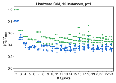
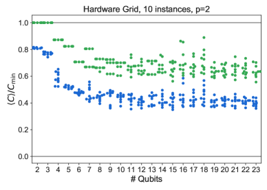
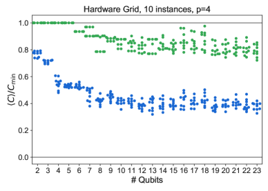
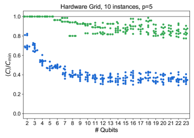
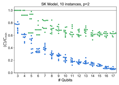
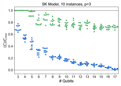
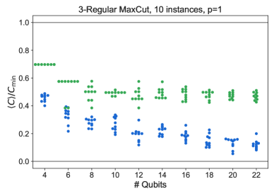
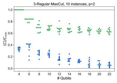
As the name implies, noisy intermediate-scale quantum (NISQ) processors are noisy devices with high error rates and a variety of error channels. Thus, NISQ circuits are expected to degrade in performance as the number of gates is increased. Here, we study the performance of QAOA as implemented on our quantum processor at different and using an application-specific metric: the normalized observed cost function . A value of is perfect and corresponds to the performance we would expect from random guessing. In order to distinguish the effects of noise from the robustness provided by using a classical outer-loop optimizer, here we report results obtained from running circuits at the theoretically optimal values.
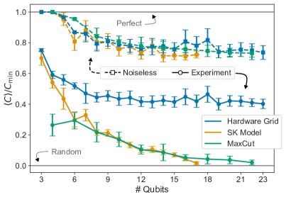
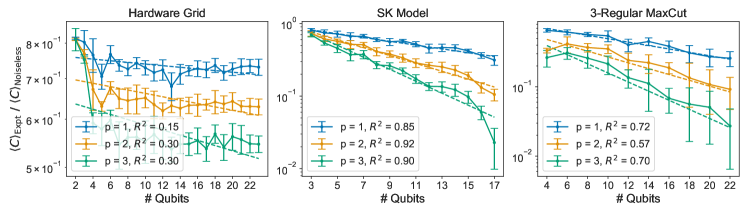
In Figure 4, we observe that achieved for the hardware graph seems to saturate to a value that is independent of of . This occurs despite the fact that circuit fidelity is decreasing with increasing . In fact, this is theoretically anticipated behavior that can be understood by moving to the Heisenberg operator formalism and considering an observable . The expectation value for this operator is conjugated by the circuit unitary involving applications of the instance graph. This gives an expression for the expectation value of which only involves qubits that are at most edges away from and . Thus for fixed , the error for a given term is asymptotically unaffected as we grow . Recall that is a sum of these terms, so the total error scales linearly with ; but so is constant with respect to . Note that non-local error channels or crosstalk could potentially remove this property.
Compiled problems—namely SK model and 3-regular MaxCut problems—result in deeper circuits extensive in the number of qubits. As the depth grows, there is a higher chance of an error occurring. The high degree of the SK model graph and the high effective degree of the MaxCut circuits after compilation means that these errors quickly propagate among all qubits and the quality of solutions can be approximately modeled as the result of a depolarizing channel, with further analysis in Appendix E. Even on these challenging problems, we observe performance exceeding random guessing for problem sizes up to 17 bits, even with circuits of depth . Note finally that despite circuits with significantly fewer gates (although similar depth), performance on the MaxCut instances tracks performance on the SK model instances rather closely, further substantiating the circuit depth as useful proxy for the performance of QAOA.
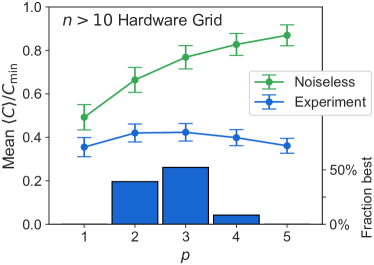
In a noiseless case, the quality of a QAOA solution can be improved by increasing the depth parameter . However, the additional depth also increases the probability of error. We study this interplay between noise and algorithmic power in Figure 5. Previously, improved performance with had only been experimentally demonstrated for an problem Bengtsson et al. (2019). For larger problems (), performance for was shown to be within error bars of the performance Pagano et al. (2019). Figure 5 shows the -dependence averaged across all 130 instances where . The mean finds its maximum at , although there are variations among the instances comparable in scale to the experimental -dependence. The relatively flat dependence of performance on depth suggests that the experimental noise seems to nearly balance the increase in theoretical performance for this problem family. For a more meaningful aggregation of the many random instances across problem sizes, we consider each instance individually and identify which value of the hyperparameter maximizes performance for that particular instance. A histogram of these per-instance maximal values is inset in Figure 5, showing that performance is maximized at for over half of instances larger than ten qubits. Note finally that our full dataset (see Appendix E) includes per-instance data at all settings of .
V Conclusion
Discrete optimization is an enticing application for near-term devices owing to both the potential value of solutions as well as the viability of heuristic low-depth algorithms such as the QAOA. While no existing quantum processors can outperform classical optimization heuristics, the application of popular methods such as the QAOA to prototypical problems can be used as a benchmark for comparing various hardware platforms.
Previous demonstrations of the QAOA have primarily optimized problems tailored to the hardware architecture at minimal depth. Using the Google “Sycamore” platform, we explored these types of problems, which we termed Hardware Grid problems, and demonstrated robust performance at large numbers of qubits. We showed that the locations of maxima and minima in the diagnostic landscape match those from the theoretically computed surface, and that variational optimization can still find the optimum with noisy quantum objective function evaluation. We also applied the QAOA to various problem sizes using pre-computed parameters from noiseless simulation, and observed an -independent noise effect on the approximation ratios for Hardware Grid problems. This is consistent with our theoretical understanding that the noise-induced degradation of each term in the objective function remains constant in the shallow-depth regime where correlations remain local. Furthermore, we report the first clear cases of performance maximization at for the QAOA owing to the low error rate of our hardware.
Most real world instances of combinatorial optimization problems cannot be mapped to hardware-native topologies without significant additional resources. Instead, problems must be compiled by routing qubits with swap networks. This additional overhead can have a significant impact on the algorithm’s performance. We studied random instances of the fully-connected SK model. Although we report non-negligible performance for large (), deep (), and complex (fully-connected) problems, we see that performance degrades with problem size for such instances.
The promise of quantum enhanced optimization will continue to motivate the development of new quantum technology and algorithms. Nevertheless, for quantum optimization to compete with classical methods for real-world problems, it is necessary to push beyond contrived problems at low circuit depth. Our work demonstrates important progress in the implementation and performance of quantum optimization algorithms on a real device, and underscores the challenges in applying these algorithms beyond those natively realized by hardware interaction graphs.
Acknowledgements
The authors thank the Cambridge Quantum Computing team for helpful correspondence about their compiler, which we used for routing of MaxCut problems. The VW team acknowledges support from the European Union’s Horizon 2020 research and innovation program under grant agreement No. 828826 “Quromorphic”. We thank all other members of the Google Quantum team, as well as our executive sponsors. Dave Bacon is a CIFAR Associate Fellow in the Quantum Information Science Program.
Author Contributions
R. Babbush and E. Farhi designed the experiment. M. Harrigan and K. Sung led code development and data collection with assistance from non-Google collaborators. Z. Jiang and N. Rubin derived the gate synthesis used in compilation. The manuscript was written by M. Harrigan, R. Babbush, E. Farhi, and K. Sung. Experiments were performed using cloud access to a quantum processor that was recently developed and fabricated by a large effort involving the entire Google Quantum team.
Code and Data Availability
The code used in this experiment is available at https://github.com/quantumlib/ReCirq. The experimental data for this experiment is available on Figshare, see Ref. 38.
References
- Arute et al. (2019) Frank Arute, Kunal Arya, Ryan Babbush, Dave Bacon, Joseph C. Bardin, Rami Barends, Rupak Biswas, Sergio Boixo, Fernando G. S. L. Brandao, David A. Buell, Brian Burkett, Yu Chen, Zijun Chen, Ben Chiaro, Roberto Collins, William Courtney, Andrew Dunsworth, Edward Farhi, Brooks Foxen, Austin Fowler, Craig Gidney, Marissa Giustina, Rob Graff, Keith Guerin, Steve Habegger, Matthew P. Harrigan, Michael J. Hartmann, Alan Ho, Markus Hoffmann, Trent Huang, Travis S. Humble, Sergei V. Isakov, Evan Jeffrey, Zhang Jiang, Dvir Kafri, Kostyantyn Kechedzhi, Julian Kelly, Paul V. Klimov, Sergey Knysh, Alexander Korotkov, Fedor Kostritsa, David Landhuis, Mike Lindmark, Erik Lucero, Dmitry Lyakh, Salvatore Mandrà, Jarrod R. McClean, Matthew McEwen, Anthony Megrant, Xiao Mi, Kristel Michielsen, Masoud Mohseni, Josh Mutus, Ofer Naaman, Matthew Neeley, Charles Neill, Murphy Yuezhen Niu, Eric Ostby, Andre Petukhov, John C. Platt, Chris Quintana, Eleanor G. Rieffel, Pedram Roushan, Nicholas C. Rubin, Daniel Sank, Kevin J. Satzinger, Vadim Smelyanskiy, Kevin J. Sung, Matthew D. Trevithick, Amit Vainsencher, Benjamin Villalonga, Theodore White, Z. Jamie Yao, Ping Yeh, Adam Zalcman, Hartmut Neven, and John M. Martinis, “Quantum supremacy using a programmable superconducting processor,” Nature 574, 505–510 (2019).
- Aspuru-Guzik et al. (2005) Alán Aspuru-Guzik, Anthony D. Dutoi, Peter J. Love, and Martin Head-Gordon, “Simulated quantum computation of molecular energies,” Science 309, 1704–1707 (2005).
- O’Malley et al. (2016) P. J. J. O’Malley, R. Babbush, I. D. Kivlichan, J. Romero, J. R. McClean, R. Barends, J. Kelly, P. Roushan, A. Tranter, N. Ding, B. Campbell, Y. Chen, Z. Chen, B. Chiaro, A. Dunsworth, A. G. Fowler, E. Jeffrey, E. Lucero, A. Megrant, J. Y. Mutus, M. Neeley, C. Neill, C. Quintana, D. Sank, A. Vainsencher, J. Wenner, T. C. White, P. V. Coveney, P. J. Love, H. Neven, A. Aspuru-Guzik, and J. M. Martinis, “Scalable quantum simulation of molecular energies,” Phys. Rev. X 6, 031007 (2016).
- Biamonte et al. (2016) Jacob Biamonte, Peter Wittek, Nicola Pancotti, Patrick Rebentrost, Nathan Wiebe, and Seth Lloyd, “Quantum machine learning,” Nature 549, 195–202 (2016).
- Lloyd (1996) Seth Lloyd, “Universal quantum simulators,” Science 273, 1073–1078 (1996).
- Kadowaki and Nishimori (1998) Tadashi Kadowaki and Hidetoshi Nishimori, “Quantum annealing in the transverse Ising model,” Phys. Rev. E 58, 5355–5363 (1998).
- Farhi et al. (2001) Edward Farhi, Jeffrey Goldstone, Sam Gutmann, Joshua Lapan, Andrew Lundgren, and Daniel Preda, “A quantum adiabatic evolution algorithm applied to random instances of an NP-complete problem,” Science 292, 472–475 (2001).
- Lucas (2014) Andrew Lucas, “Ising formulations of many NP problems,” Frontiers in Physics 2, 5 (2014).
- Barahona (1982) F Barahona, “On the computational complexity of Ising spin glass models,” Journal of Physics A: Mathematical and General 15, 3241–3253 (1982).
- Choi (2008) Vicky Choi, “Minor-embedding in adiabatic quantum computation: I. the parameter setting problem,” Quantum Information Processing 7, 193–209 (2008).
- Denchev et al. (2016) Vasil S. Denchev, Sergio Boixo, Sergei V. Isakov, Nan Ding, Ryan Babbush, Vadim Smelyanskiy, John Martinis, and Hartmut Neven, “What is the computational value of finite-range tunneling?” Phys. Rev. X 6, 031015 (2016).
- Farhi et al. (2014a) Edward Farhi, Jeffrey Goldstone, and Sam Gutmann, “A quantum approximate optimization algorithm,” (2014a), arXiv:1411.4028 [quant-ph] .
- Farhi et al. (2014b) Edward Farhi, Jeffrey Goldstone, and Sam Gutmann, “A quantum approximate optimization algorithm applied to a bounded occurrence constraint problem,” (2014b), arXiv:1412.6062 [quant-ph] .
- Biswas et al. (2017) Rupak Biswas, Zhang Jiang, Kostya Kechezhi, Sergey Knysh, Salvatore Mandrà, Bryan O’Gorman, Alejandro Perdomo-Ortiz, Andre Petukhov, John Realpe-Gómez, Eleanor Rieffel, Davide Venturelli, Fedir Vasko, and Zhihui Wang, “A NASA perspective on quantum computing: Opportunities and challenges,” Parallel Computing 64, 81–98 (2017).
- Wecker et al. (2016) Dave Wecker, Matthew B. Hastings, and Matthias Troyer, “Training a quantum optimizer,” Phys. Rev. A 94, 022309 (2016).
- Farhi and Harrow (2016) Edward Farhi and Aram W Harrow, “Quantum supremacy through the quantum approximate optimization algorithm,” (2016), arXiv:1602.07674 [quant-ph] .
- Jiang et al. (2017) Zhang Jiang, Eleanor G. Rieffel, and Zhihui Wang, “Near-optimal quantum circuit for Grover’s unstructured search using a transverse field,” Phys. Rev. A 95, 062317 (2017).
- Wang et al. (2018) Zhihui Wang, Stuart Hadfield, Zhang Jiang, and Eleanor G. Rieffel, “Quantum approximate optimization algorithm for MaxCut: A fermionic view,” Phys. Rev. A 97, 022304 (2018).
- Hadfield et al. (2017) Stuart Hadfield, Zhihui Wang, Bryan O’Gorman, Eleanor Rieffel, Davide Venturelli, and Rupak Biswas, “From the quantum approximate optimization algorithm to a quantum alternating operator ansatz,” Algorithms 12, 34 (2017).
- Lloyd (2018) Seth Lloyd, “Quantum approximate optimization is computationally universal,” (2018), arXiv:1812.11075 [quant-ph] .
- Farhi et al. (2019) Edward Farhi, Jeffrey Goldstone, Sam Gutmann, and Leo Zhou, “The quantum approximate optimization algorithm and the Sherrington-Kirkpatrick model at infinite size,” (2019), arXiv:1910.08187 [quant-ph] .
- Otterbach et al. (2017) J. S. Otterbach, R. Manenti, N. Alidoust, A. Bestwick, M. Block, B. Bloom, S. Caldwell, N. Didier, E. Schuyler Fried, S. Hong, P. Karalekas, C. B. Osborn, A. Papageorge, E. C. Peterson, G. Prawiroatmodjo, N. Rubin, Colm A. Ryan, D. Scarabelli, M. Scheer, E. A. Sete, P. Sivarajah, Robert S. Smith, A. Staley, N. Tezak, W. J. Zeng, A. Hudson, Blake R. Johnson, M. Reagor, M. P. da Silva, and C. Rigetti, “Unsupervised machine learning on a hybrid quantum computer,” (2017), arXiv:1712.05771 [quant-ph] .
- Willsch et al. (2019) Madita Willsch, Dennis Willsch, Fengping Jin, Hans De Raedt, and Kristel Michielsen, “Benchmarking the quantum approximate optimization algorithm,” (2019), arXiv:1907.02359 [quant-ph] .
- Abrams et al. (2019) Deanna M. Abrams, Nicolas Didier, Blake R. Johnson, Marcus P. da Silva, and Colm A. Ryan, “Implementation of the XY interaction family with calibration of a single pulse,” (2019), arXiv:1912.04424 [quant-ph] .
- Bengtsson et al. (2019) Andreas Bengtsson, Pontus Vikstål, Christopher Warren, Marika Svensson, Xiu Gu, Anton Frisk Kockum, Philip Krantz, Christian Križan, Daryoush Shiri, Ida-Maria Svensson, Giovanna Tancredi, Göran Johansson, Per Delsing, Giulia Ferrini, and Jonas Bylander, “Quantum approximate optimization of the exact-cover problem on a superconducting quantum processor,” (2019), arXiv:1912.10495 [quant-ph] .
- Pagano et al. (2019) G. Pagano, A. Bapat, P. Becker, K. S. Collins, A. De, P. W. Hess, H. B. Kaplan, A. Kyprianidis, W. L. Tan, C. Baldwin, L. T. Brady, A. Deshpande, F. Liu, S. Jordan, A. V. Gorshkov, and C. Monroe, “Quantum approximate optimization with a trapped-ion quantum simulator,” (2019), arXiv:1906.02700 [quant-ph] .
- Qiang et al. (2018) Xiaogang Qiang, Xiaoqi Zhou, Jianwei Wang, Callum M. Wilkes, Thomas Loke, Sean O’Gara, Laurent Kling, Graham D. Marshall, Raffaele Santagati, Timothy C. Ralph, Jingbo B. Wang, Jeremy L. O’Brien, Mark G. Thompson, and Jonathan C. F. Matthews, “Large-scale silicon quantum photonics implementing arbitrary two-qubit processing,” Nature Photonics 12, 534–539 (2018).
- The Cirq Developers (2020) The Cirq Developers, “Cirq: A python framework for creating, editing, and invoking noisy intermediate scale quantum (NISQ) circuits,” (2020), https://github.com/quantumlib/Cirq.
- Rønnow et al. (2014) Troels F. Rønnow, Zhihui Wang, Joshua Job, Sergio Boixo, Sergei V. Isakov, David Wecker, John M. Martinis, Daniel A. Lidar, and Matthias Troyer, “Defining and detecting quantum speedup,” Science 345, 420–424 (2014).
- Sherrington and Kirkpatrick (1975) David Sherrington and Scott Kirkpatrick, “Solvable model of a spin-glass,” Phys. Rev. Lett. 35, 1792–1796 (1975).
- Hirata et al. (2011) Yuichi Hirata, Masaki Nakanishi, Shigeru Yamashita, and Yasuhiko Nakashima, “An efficient conversion of quantum circuits to a linear nearest neighbor architecture,” Quantum Info. Comput. 11, 142–166 (2011).
- Goemans and Williamson (1995) Michel X. Goemans and David P. Williamson, “Improved approximation algorithms for maximum cut and satisfiability problems using semidefinite programming,” J. ACM 42, 1115–1145 (1995).
- Bravyi et al. (2019) Sergey Bravyi, Alexander Kliesch, Robert Koenig, and Eugene Tang, “Obstacles to state preparation and variational optimization from symmetry protection,” (2019), arXiv:1910.08980 [quant-ph] .
- Cowtan et al. (2019) Alexander Cowtan, Silas Dilkes, Ross Duncan, Alexandre Krajenbrink, Will Simmons, and Seyon Sivarajah, “On the qubit routing problem,” (2019), arXiv:1902.08091 [quant-ph] .
- Yang et al. (2017) Zhi-Cheng Yang, Armin Rahmani, Alireza Shabani, Hartmut Neven, and Claudio Chamon, “Optimizing variational quantum algorithms using Pontryagin’s minimum principle,” Phys. Rev. X 7, 021027 (2017).
- McClean et al. (2018) Jarrod R. McClean, Sergio Boixo, Vadim N. Smelyanskiy, Ryan Babbush, and Hartmut Neven, “Barren plateaus in quantum neural network training landscapes,” Nature Communications 9, 4812 (2018).
- (37) Kevin J. Sung, Matthew P. Harrigan, Nicholas Rubin, Zhang Jiang, Ryan Babbush, and Jarrod McClean, “Practical optimizers for variational quantum algorithms,” in preparation .
- Quantum and Collaborators (2020) Google AI Quantum and Collaborators, “Sycamore QAOA experimental data,” (2020), 10.6084/m9.figshare.12597590.v2.
- Zhang et al. (2003) Jun Zhang, Jiri Vala, Shankar Sastry, and K. Birgitta Whaley, “Geometric theory of nonlocal two-qubit operations,” Phys. Rev. A 67, 042313 (2003).
Appendix A Hardware and Compilation Details
In this section, we discuss detailed compilation of the desired unitaries into the hardware native gateset, particularly the syc gate defined in Figure 2c. The syc gate is similar to the gate used in Arute et al. (2019) but with the conditional phase tuned to be precisely . A gate is simultaneously calibrated and available but has a longer gate duration and requires additional (physical) Z rotations to match phases. The required interactions for this study are compiled to an equivalent number of syc and , so syc was used in all circuits. Single-qubit microwave pulses enact “Phased X” gates (alternatively called XY rotations or the W gate) with corresponding to and corresponding to (up to global phase). Intermediate values of control the axis of rotation in the X-Y plane of the Bloch sphere.
Arbitrary single-qubit rotations can be applied by a gate followed by a gate. As a compilation step, we merge adjacent single-qubit operations to be of this form. Therefore, our circuit is structured as a repeating sequence of: a layer of PhX gates; a layer of gates; and a layer of syc gates. All Z rotations of the form can be efficiently commuted through syc and PhX to the end of the circuit and discarded. This leaves alternating layers of PhX and syc gates. The overheads of compilation are summarized in Table S1.
| Problem | Routing | Interaction | Synthesis |
|---|---|---|---|
| Hardware Grid | WESN | 2 | |
| MaxCut | Greedy | 2 | |
| MaxCut | Greedy | swap | 3 |
| SK Model | Swap Network | 3 |
Compilation of . These interactions (used for Hardware Grid and MaxCut problems) can be compiled with 2 layers of syc gates and 2+1 associated layers of single qubit PhX gates. We report the required number of single-qubit layers as 2+1 because the initial (or final) layer from one set of interactions can be merged into the final (initial) single qubit gate layer of the preceding (following) set of interactions. In general, the number of single qubit layers will be equivalent to the number of two-qubit gate layers with one additional single-qubit layer at the beginning of the circuit and one additional single-qubit layer at the end of the circuit. The explicit compilation of to syc is available in Cirq and a proof can be found in the supplemental material of Ref. Arute et al. (2019). Here we reproduce the derivation in slightly different notation but following a similar motivation.
The syc gate is an fSim(,) which can be broken down into a , cz, swap, and two S gates according to Figure S1.

We analyze the KAK coefficients for a composite gate of two syc gates sandwiching arbitrary single qubit rotations, depicted in Figure S2, to determine the space of gates accessible with two syc gates.

Any two qubit gate is locally equivalent to standard KAK form Zhang et al. (2003). The coefficients in the KAK form is equivalent to the operator Schmidt coefficients of the 2-qubit unitary. To find the Schmidt coefficients, we introduce the matrix representation of 2-qubit gates in terms of Pauli operators, i.e., the -th matrix element equals to the corresponding coefficient of the Pauli operator , where ,
| (6) |
The Schmidt coefficients of equal to the singular values of . Any single-qubit gate can be decomposed into the -- rotations; the rotations commute with the cz and the cphase, and they do not affect the Schmidt coefficients of the two-qubit operation defined in Figure S2. We neglect the rotations and simplify to single-qubit rotations
| (7) |
The Pauli matrix representation of in Eq. (7) is
| (8) |
where and . The rank of the matrix is one, representing a product unitary. After being conjugated by the cz gates, i.e, , the matrix becomes
| (9) |
where we use the relations for ,
| (10) |
The cphase part in the syc gate is
| (11) |
where . An arbitrary operator left and right multiplied by cphase part is expressed as
| (12) |
Applying the operation to the operator , we have
| (13) |
Applying the operation to the operator , we have
| (14) |
The resulting two-qubit gate at the output of the circuit in Figure S2 takes the form
| (15) |
Two singular values of are and corresponding to the diagonal matrix elements and , and the magnitudes of these two singular values are bounded by the angle . Consider the two-dimensional subspace of the matrix , , and with the two known singular values removed
| (16) |
The Pauli representation matrix in the reduced space is
| (17) | ||||
| (18) |
To calculate the singular values of a matrix
| (19) |
we used the formula
| (20) |
where and . For matrix , we have,
| (21) | ||||
| (22) | ||||
| (23) |
and
| (24) | ||||
| (25) |
We have solved all the four singular values of the 2-qubit unitary at the output of Figure S1,
| (26) |
For the case and , we have and the other two singular values
| (27) |
Since , we can implement any cphase gate using only two syc gates. This is achieved by matching the Schmidt coefficients of to and . If then we can reset and appropriately to select out the other pair of singular values.
Compilation of swap. A swap gate requires three applications of syc and is used for the 3-regular MaxCut problem circuits. The swap gate was numerically compiled by optimizing the angles of the circuit in Figure S3 to match the KAK interaction coefficients for the swap gate.
After the the angles in the circuit depicted in Figure S3 are determined to match the KAK coefficient of the swap gate we add single qubit rotations to make the circuit fully equivalent to swap.
Compilation of . This composite interaction can be effected with three applications of syc and is used for SK-model circuits. The syc gate KAK coefficients are which is locally equivalent to a followed by a swap. Therefore, to implement a followed by a swap we need to apply a single syc gate followed by the composite . The total composite gate now involves 3 syc gates, a single gate and two gates.
Scheduling of Hardware Grid gates. An efficient planar graph edge-coloring can be used to schedule as many simultaneous interactions as possible. We activate links on the graph in the following order:
1) horizontal edges starting from even nodes;
2) horizontal edges starting from odd nodes;
3) vertical edges starting from even nodes;
4) vertical edges starting from odd nodes.
Viewed as cardinal directions and choosing an even node as the central point this corresponds to a west, east, south, north (W, E, S, N) activation sequence.

Fully Connected Swap Network. All-to-all interactions can be implemented optimally with a swap network in which pairs of linear-nearest-neighbor qubits are repeatedly interacted and swapped. Crucially, the required interactions swap and between all pairs all mutually commute so we are free to re-order all two-qubit interactions to minimize compiled circuit depth. After applications of layers of interactions (alternating between even and odd qubits), every qubit has been involved in a interaction with every other qubit and logical qubit indices have been reversed. This can be viewed as a (parallel) bubble sort algorithm initialized with a reverse-sorted list of logical qubit indices. An example at is shown in Figure S4. If is even, two applications of the swap network return qubit indices to their original mapping. Otherwise, post-processing can reverse the measured bitstrings.
The swap network requires linear connectivity. On the 23-qubit subgraph of the Sycamore device used for this experiment, this limits us to a maximum size of for the SK model, shown in Figure S5.
Appendix B Prior Work
| Reference | Date | Problem topology | Optimization | |||
|---|---|---|---|---|---|---|
| Otterbach et al. (2017) | 2017-12 | Hardware | 3 | 19 | 1 | Yes |
| Qiang et al. (2018) | 2018-08 | Hardware | 1 | 2 | 1 | No |
| Pagano et al. (2019) | 2019-06 | Hardware1 (system 1) | 12, 20 | 1 | Yes | |
| Hardware1 (system 2) | 20–40 | 1–2(2) | No | |||
| Willsch et al. (2019) | 2019-07 | Hardware | 3 | 8 | 1 | No |
| Abrams et al. (2019) | 2019-12 | Ring | 2 | 4 | 1 | No |
| Fully-connected | No | |||||
| Bengtsson et al. (2019) | 2019-12 | Hardware | 1 | 2 | 1, 2 | Yes |
| This work | Hardware | 4 | 2–23 | 1–5 | Yes | |
| 3-regular | 3 | 4–22 | 1–3 | Yes | ||
| Fully-connected | 3–17 | 1–3 | Yes |
Prior work has included experimental demonstration of the QAOA. The referenced works often include additional results, but we focus specifically on the sections dealing with experimental implementation of the algorithm.
Otterbach et al. (2017) demonstrated a Bayesian optimization of p = 1 parameters on a 19-bit hardware-native Ising graph using a Rigetti superconducting qubit processor. The authors compared the cumulative probability of finding the lowest energy bitstring over the course of the optimization to binomial coin flips and showed performance from the device exceeding random guessing. The problem topology involved a roughly hexagonal tessellation. The problems were related to a restricted form of two-class clustering.
Qiang et al. (2018) demonstrated a , QAOA landscape on their photonic quantum processor. They presented three instances of the two-bit problem, which was framed as Max2Xor. The color scale for the landscapes was re-scaled for experimental values. They demonstrated high probability of obtaining the correct bitstrings.
Pagano et al. (2019) demonstrated application of the QAOA with two ion trap quantum processors, called “system 1” and “system 2”. The problems were of the form with close to unity. This corresponds to an antiferromagnetic 1D chain. This problem is fully connected, but is spiritually similar to the hardware native planar graphs studied in superconducting architectures in the sense that the cost function cannot be programmed and is easily solvable at any system size. A landscape is shown for from system 1. Optimization traces are shown for and on system 1. On system 2, performance was demonstrated at optimal parameters for . Additionally, a partial grid search was performed on system 2. Nine discrete choices for were selected and then a scan over was reported for each choice. Finally, on system 2, performance was compared between and at , giving a ratio of versus , respectively.
Willsch et al. (2019) demonstrated an application of the QAOA via IBM’s Quantum Experience cloud service on the 16Q Melbourne device. The 8-bit problem studied was framed as 2SAT and had a topology matching the device with maximum node degree of 3. A landscape with re-scaled color map was compared to the theoretical landscape.
Abrams et al. (2019) implemented QAOA on two types of problems; each with two compilation strategies. The 4-bit problems had a ring topology and a fully-connected topology. While a 4-qubit ring would fit on the Rigetti superconducting device, they implemented both problems using only linear connectivity with the introduction of swaps. In one compilation strategy, they used cz as the gate-synthesis target. In the other, they used both cz and . The color bars were re-scaled for the experimental data.
Bengtsson et al. (2019) ran 2-bit QAOA instances on their superconducting architecture at and . They show four landscapes and demonstrate optimization for . They observed that increasing circuit depth to increases the probability of observing the correct bitstring.
Appendix C Readout correction
The experimentally measured expectation values plotted in Figure 3 were adjusted with a procedure used to compensate for qubit readout error. We model readout error as a classical bit-flip error channel that changes the measurement result of qubit from 0 to 1 with probability and from 1 to 0 with probability . Under the effect of this error channel, a measurement of a single qubit in the computational basis is described by the following positive operator-valued measure (POVM) elements (we drop the subscript here for clarity):
| (28) | ||||
| (29) |
where , . The uncorrected observable can be written as
| (30) |
Solving for , we have
| (31) |
For our problems we are interested in the two-qubit observable , so the corrected observable is
| (32) |
This expression tells us how to adjust the measured observable to compensate for the readout error. In the above analysis, we can replace and by their average if we perform measurements in the following way: for half of the measurements, apply a layer of gates immediately before measuring, and then flip the measurement results. In this case, the corrected observable is
| (33) |
We estimated the value of on the device by preparing and measuring the qubit in the state 1,000,000 times and counting how often a 1 was measured; was estimated in the same way but by preparing the state instead of the zero state. This estimation was performed periodically during the data collection for Figure 3 to account for drift following automated calibration.
We measure each qubit via the state-dependent dispersive shift they induce on their corresponding harmonic readout resonator as described in Arute et al. (2019) supplementary information section III. We interrogate the readout resonator frequency with an appropriately calibrated microwave pulse (e.g. a frequency, power, and duration). When demodulated, the readout signal produces a ‘cloud’ of In-phase and Quadrature (IQ) Voltage points which are used to train an out state descrimator. Often, we find that optimal single-qubit calibrations extend to the case of simultaneous readout, but this is not always the case. For example, due to the Stark shift induced by photons in readout resonators, new frequency collisions may be introduced that are not present in the isolated readout case. Similarly, the combined power of a multiplexed readout pulses may exceed the saturation power of our parametric amplifier.
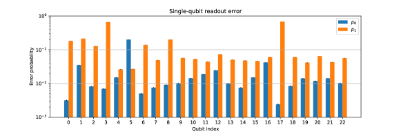
At the time of the primary data collection for this experiment, all automated calibration routines were performed with each qubit in isolation. Subsequently, a calibration which optimizes qubit detunings during readout was implemented to mitigate these correlated readout errors caused by frequency collisions. Figure S6 shows and state errors for simultaneous readout of all 23 qubits (which are used to correct observables) both as they were during primary data taking for Figure 3 (top) and after implementing the improved readout detuning calibration (bottom). During primary data collection, the median isolated readout error was 4.4% as measured during the previous automated calibration. The discrepancy between these figures and the calibration values shown in Figure S6, top can be attributed to drift since the automated system calibration in addition to the simultaneity effects described above.
Data presented in Figure 4 and Figure 5 was taken on a different date with median isolated readout error as 4.1% as reported in the main text. Readout correction was not used for these two figures.
While automated calibrations will continue to improve, drift will likely remain an inevitability when controlling qubits with analog signals. As such, we expect the readout corrections employed here will continue to provide utility for end-users of cloud-accessible devices. In general, there will always be a difference between a hands-on calibration conducted by an experimental physicist and automated calibration for a cloud-accessible device, and we look forward to future research ideas being “productionized” to make them accessible to a wide audience of algorithms researchers. Even in this instance there is still an imperfect abstraction: if one is interested in reading only a subset of all available qubits, higher performance can be obtained by doing a highly-tailored calibration; but we expect that the vast majority of cases will be served better by the new calibration routines.
Appendix D Optimizer Details
In this section, we describe the classical optimization algorithm that we used to obtain the optimization results presented in Figure 3. The algorithm is a variant of gradient descent which we call “Model Gradient Descent”. In each iteration of the algorithm, several points are randomly chosen from the vicinity of the current iterate. The objective function is evaluated at these points, and a quadratic model is fit to the graph of these points and previously evaluated points in the vicinity using least-squares regression. The gradient of this quadratic model is then used as a surrogate for the true gradient, and the algorithm descends in the corresponding direction. Our implementation includes hyperparameters that determine the rate of descent, the radius of the vicinity from which points are sampled (the sample radius), the number of points to sample, and optionally, whether and how quickly the rate of descent and the sample radius should decay as the algorithm proceeds. Pseudocode is given in Algorithm 1.
Appendix E Supporting Plots for Performance at Optimal Angles
E.1 Analysis of Noise
There are two relevant mechanisms when considering the difference in performance between problems. One is the propagation of faults through the circuit and the other is fidelity decay due to circuit depth. A single fault on low-degree problems (Hardware Grid and 3-regular MaxCut, with degree four and three, respectively) can only propagate to terms edges away from the original location of the fault, irrespective of the total number of qubits. However, if compilation results in circuits extensive in the system size, the probability of a fault increases. For the SK-model, the degree of the problem is extensive in system size so both the propensity for fault propagation as well as the probability of faults grows with . Additionally, compilation of the 3-regular problems onto the hardware topology introduces SWAPs, which can propagate faults through nodes which would otherwise not be adjacent in the problem graph.
To probe these two effects, we fit a global depolarizing channel to the results for the three problems. A global depolarizing channel results in the mixed state
where is the noiseless QAOA state, is the -qubit identity matrix, and is the total circuit fidelity. because of the structure of the cost function, so the experimental objective function is simply a scaled version of the noiseless version, . We perform a linear regression on where and are fittable parameters physically corresponding to a per-qubit fidelity and a qubit-independent offset. For the Hardware Grid, a depolarizing model is inappropriate, as the limited fault propagation and fixed circuit depth yield a largely -independent noise signature. The exponential decay expected from a global depolarizing channel reasonably fits both the SK model and MaxCut results. We note that the fit is considerably stronger for the high-degree SK model where faults are rapidly mixed.