Partial equilibration of anti-Pfaffian edge modes at $\nu=5/2$

Abstract

The thermal Hall conductance $K$ of the fractional quantum Hall state at filling fraction $\nu=5/2$ has recently been measured to be $K=2.5\pi^{2}k_{B}^{2}T/3h$ [M. Banerjee et al., Nature 559, 205 (2018)]. The half-integer value of this result (in units of $\pi^{2}k_{B}^{2}T/3h$) provides strong evidence for the presence of a Majorana edge mode and a corresponding quantum Hall state hosting quasiparticles with non-Abelian statistics. Whether this measurement points to the realization of the PH-Pfaffian or the anti-Pfaffian state has been the subject of debate. Here we consider the implications of this measurement for anti-Pfaffian edge-state transport. We show that in the limit of a strong Coulomb interaction and an approximate spin degeneracy in the lowest Landau level, the anti-Pfaffian state admits low-temperature edge phases that are consistent with the Hall conductance measurements. These edge phases can exhibit fully-equilibrated electrical transport coexisting with partially-equilibrated heat transport over a range of temperatures. Through a study of the kinetic equations describing low-temperature electrical and heat transport of these edge states, we determine regimes of parameter space, controlling the interactions between the different edge modes, that agree with experiment.

1 Introduction

Since the discovery of the quantum Hall plateau at filling fraction $\nu=5/2$ [1], the nature of the ground state of this system has been the subject of debate. Numerical studies point toward either the Moore-Read Pfaffian state [2, 3] or its particle-hole conjugate, the anti-Pfaffian state [4, 5], as the true ground state of the system [6, 7, 8, 9, 10]. Both of these states host quasiparticles with non-Abelian statistics. On the other hand, quantum point contact tunneling experiments [11, 12, 13, 14, 15] support either the anti-Pfaffian state, the $SU(2)_{2}$ state, or the Abelian $331$ or $113$ states. Observation of upstream neutral modes [16, 17] only hints at the realization of a non-Abelian state.

As first pointed out by Kane and Fisher [18], the thermal Hall conductance $K$ provides a sensitive probe of the topological order of a fractional quantum Hall (FQH) state. $K/T$ equals the difference in the number of right and left moving chiral edge modes (in units of $\kappa_{0}=\frac{\pi^{2}k_{B}^{2}}{3h}$ at temperature $T$) for an Abelian quantum Hall state; more generally, $K$ is determined by the chiral central charge $c_{-}=c_{R}-c_{L}$ of the edge states [19] ($c_{R/L}$ is the sum of the right/left, i.e., holomorphic/anti-holomorphic, central charges of the edge modes). Consequently, the remarkable measurement of Banerjee et al. [20] that finds $K=2.5\kappa_{0}T$ at $\nu=5/2$ provides strong evidence for a non-Abelian quantum Hall state. Taken at face value, this result suggests the recently proposed topological order, the particle-hole symmetric Pfaffian state (PH-Pfaffian) [21] which has chiral central charge $c_{-}=5/2$, is realized. One explanation [22] for the apparent contradiction between this experimental result and prior numerical work invokes disorder and Landau Level mixing, which are inevitably present in any real sample, but difficult to include in numerics. Another scenario is that long-range disorder results in puddles of Pfaffian and anti-Pfaffian states, which (intuitively) contribute $(c_{-}^{\rm Pfaffian}+c_{-}^{\rm anti-Pfaffian})/2=(7/2+3/2)/2$ to the thermal Hall conductance. The resulting state can exhibit the thermal Hall conductance of $K=2.5\kappa_{0}T$ in some parameter regimes [23, 24, 25]. However, the conditions for this observation were found to be rather restrictive.

Simon [26] has proposed an alternative interpretation: The experimental measurement may not directly reflect the bulk topological order; instead $K=2.5\kappa_{0}T$ may be due to suppressed thermal equilibration relative to charge equilibration of anti-Pfaffian edge modes. This partial equilibration is believed to occur at $\nu=2/3$ and potentially $\nu=8/3$ [27, 20]. The distinction between various candidate $\nu=5/2$ states, based on the thermal Hall conductance, is clear only if the different edge channels of the quantum Hall sample are well equilibrated with each other. If instead there’s no equilibration between edge modes, the thermal Hall conductance is proportional to the total central charge $c=c_{R}+c_{L}$ of the edge state. If the edge modes only partially equilibrate, the thermal Hall conductance can in principle take any value between the fully-equilibrated conductance and the non-equilibrated one. (These statements are true only if ideal contacts are assumed [28, 29].) The Pfaffian state has three bosonic modes and one Majorana mode (with central charge $c^{\rm Majorana}=1/2$), all moving “downstream” along the edge. Assuming the contacts are ideal, the resulting thermal Hall conductance equals $K=\frac{7}{2}\kappa_{0}T$, which is not consistent with the measurement $K=2.5\kappa_{0}T$. The anti-Pfaffian state has three “downstream” bosonic modes, one “upstream” bosonic mode, and one “upstream” Majorana mode. Therefore, depending on the degree of equilibration, the thermal Hall conductance of the anti-Pfaffian state can take any value between $K={3\over 2}\kappa_{0}T$ and $K={9\over 2}\kappa_{0}T$. Since the electrical Hall conductance $G={5\over 2}\sigma_{0}$ [20] ($\sigma_{0}=e^{2}/h$), realization of this idea requires partial thermal equilibration simultaneous with full charge equilibration, at least of the edge modes belonging to the first Landau level.

There have been a variety of different scenarios proposed for partial equilibration of the anti-Pfaffian edge state. Simon [26] originally suggested that the low velocity of the Majorana mode combined with long-range disorder might hinder the equilibration of the Majorana mode with the rest of the edge modes. However, it has been argued that the parameter regime required by this interpretation is not realized experimentally [30, 20]. Partial equilibration in the anti-Pfaffian state can also occur if the modes in the lowest Landau level do not equilibrate with modes in the first Landau level. One possible realization was described by Ma and Feldman [31]. Another mechanism whereby equilibration of the Majorana mode is suppressed was proposed by Simon and Rosenow [32]. There, equilibration between edge modes was assumed to be dominated by scattering via intermediate tunneling to Majorana zero modes localized in the bulk, rather than charge tunneling along the edge, considered in [26, 30, 31].

In this note, we continue the study of the role of equilibration in anti-Pfaffian edge-state transport. In contrast to [26, 32], we assume that electron tunneling, induced by short-range disorder, serves to equilibrate the edge modes. Tunneling between spin-up and spin-down edge modes of the lowest Landau level plays a prominent role in our scenario. These tunnelings were not considered in the previous analysis [31] of transport in the anti-Pfaffian state, as it was argued that weak spin-orbit coupling suppresses such tunnelings. The effective theories we consider are driven by such spin-flip interactions. The resulting low-energy edge states have an approximate spin symmetry in the lowest Landau level that we show can serve to suppress thermal equilibration while simultaneously allowing complete charge equilibration over a range of experimentally-relevant temperatures, in the presence of a strong Coulomb interaction.

We analyze charge and heat equilibration when the edge modes are biased at different temperatures and voltages. While we consider the effects of bias in temperature and voltage only to linear order, including higher order contributions can have interesting consequences. It has been argued that the interplay between the electrical and the thermal transport can generate distinct shot noise profiles along the Hall bar edge [33, 34, 35, 36]. These noise profiles fall into three universality classes depending on the chirality structure of the edge modes. Specifically, it has been suggested that the universality class for the noise profile of the anti-Pfaffian state is different from that of the Pfaffian and the PH-Pfaffian states, and so the measurement of shot noise along the edge of the quantum Hall system at filling fraction $\nu=5/2$ is another tool that can be used to distinguish between the different candidates.

We start in Section 2.1 with a review of the general framework that we use in order to examine the transport of charge and heat in the anti-Pfaffian state. Starting from the effective field theory of a general quantum Hall edge state, we derive the equations that describe charge and heat transport in the ohmic regime. In Section 2.2 we discuss the simple example of transport along the $\nu=2$ quantum Hall edge; this example illustrates the possible importance of an approximate spin symmetry in the lowest Landau level and helps to motivate the anti-Pfaffian edge phases considered in the remainder of the paper. In Section 2.3 we describe how we model the contacts and calculate the electrical and thermal conductance. In Section 3 we discuss the edge theory of the anti-Pfaffian state. We identify low-temperature fixed points of this theory that we argue to be relevant to experiment and discuss two of the fixed points that are driven by spin-flip tunneling. In Section 4 we apply the framework presented in Section 2.1 to these low-energy fixed points. We calculate the electrical and thermal conductances for each of these theories and discuss the regime of parameters consistent with the measured electrical $G=2.5\sigma_{0}$ and thermal $K=2.5\kappa_{0}T$ conductances. We discuss the degree to which such parameter regimes are realistic. Finally, in Section 5 we examine quantum point contact tunneling in the anti-Pfaffian state in the vicinity of these low-energy edge states.

Throughout this paper, we use the notation $\sigma_{0}=\frac{e^{2}}{h}$ and $\kappa_{0}=\frac{\pi^{2}k_{B}^{2}}{3h}$. However, for our calculations we use units where $e=\hbar=k_{B}=1$ so that $\sigma_{0}=\frac{1}{2\pi}$ and $\kappa_{0}=\frac{\pi}{6}$.

2 Edge-state transport for an Abelian quantum Hall state

2.1 Hydrodynamic kinetic equations

In this section we derive the kinetic equations that describe the low-temperature dc transport of charge and heat along the edge of an Abelian quantum Hall state, closely following [37, 38, 39, 28, 40]. We highlight the dependence of these equations on the low-temperature state of the edge modes. These equations are readily generalized to the anti-Pfaffian edge theory, which includes a chiral Majorana fermion.

Consider a layered quantum Hall state with filling fraction $\nu_{i}$ for each layer $i=1,\ldots,N$. The action for the chiral boson edge modes $\phi_{i}$ is $S_{\text{edge}}=S_{0}+S_{\text{tunneling}}$ where

$$S_{0} =-\frac{1}{4\pi}\int_{t,x}\left[\sum_{i}\frac{1}{\nu_{i}}\partial_{x}\phi_{i}(\eta_{i}\partial_{t}\phi_{i}+v_{i}\partial_{x}\phi_{i})+\sum_{i\neq j}v_{ij}\partial_{x}\phi_{i}\partial_{x}\phi_{j}\right],$$ (2.1a)

$$S_{\text{tunneling}} =-\int_{t,x}\sum_{p\in P}\left[\xi_{p}(x)\operatorname{e}^{i\sum_{j}^{N}m^{(p)}_{j}\phi_{j}}+\text{h.c.}\right].$$ (2.1b)

Here, $v_{ij}$ parameterizes the short-ranged Coulomb interaction coupling the edge-mode charge densities ${1\over 2\pi}\partial_{x}\phi_{i}$; the velocities $v_{i}$ are non-negative; $\eta_{i}=\pm 1$ denotes the chirality of the edge mode ($\eta_{i}=+1$ is a right-moving or “downstream” mode, while $\eta_{i}=-1$ is a left-moving or “upstream” mode); $\int_{t,x}=\int dtdx$; $P$ is the set of charge-conserving processes that tunnel $\nu_{j}m_{j}^{(p)}$ electrons/bosons between the edge channels; and $\xi_{p}$ is a Gaussian random field with statistical average $\overline{\xi_{p}(x)\xi^{*}_{p^{\prime}}(x^{\prime})}=\delta_{pp^{\prime}}W_{p}\delta(x-x^{\prime})$. To study the transport properties of $S_{\text{edge}}$ it’s convenient to diagonalize $S_{0}$ using the transformation $\phi_{i}=\Lambda_{i\alpha}\tilde{\phi}_{\alpha}$:

$$S_{0} =-\frac{1}{4\pi}\int_{t,x}\left[\sum_{\alpha}\partial_{x}\tilde{\phi}_{\alpha}(\tilde{\eta}_{\alpha}\partial_{t}\tilde{\phi}_{\alpha}-\tilde{v}_{\alpha}\partial_{x}\tilde{\phi}_{\alpha})\right].$$ (2.2)

This transformation is of the form $\Lambda_{i\alpha}=\sqrt{\nu_{i}}\tilde{\Lambda}_{i\alpha}$ where $\tilde{\Lambda}_{i\alpha}$ satisfies $\tilde{\Lambda}^{T}\eta\tilde{\Lambda}=\eta$ ($\eta_{ij}=\delta_{ij}\eta_{i}$). Note that $\tilde{v}_{\alpha}\geq 0$, $\eta_{\alpha}=\pm 1$, and $\sum_{i}\eta_{i}=\sum_{\alpha}\eta_{\alpha}$. Throughout this paper, we will use Latin indices $i,j$ for the fractional modes and Greek indices $\alpha,\beta,\gamma$ for the bosonic modes that diagonalize the action.

The leading order renormalization group equation for the variance $W_{p}$ is

$$\frac{dW_{p}}{dl}=(3-2\Delta_{p})W_{p}$$ (2.3)

with $\Delta_{p}$ the scaling dimension of the tunneling operator ${\cal O}_{p}=\operatorname{e}^{i\sum_{j}m^{(p)}_{j}\phi_{j}}=\operatorname{e}^{i\sum_{j,\alpha}m^{(p)}_{j}\Lambda_{j\alpha}\tilde{\phi}_{\alpha}}$. When all tunneling operators appearing in $S_{\text{tunneling}}$ are irrelevant, $\Delta_{p}>\frac{3}{2}$, the fixed point action is $S_{0}$. At zero temperature, the currents $\tilde{I}_{\alpha}=-\frac{1}{2\pi}\partial_{t}\tilde{\phi}_{\alpha}$ and $\tilde{J}_{\alpha}(x)=\frac{\eta_{\alpha}}{4\pi}(\partial_{t}\tilde{\phi}_{\alpha})^{2}$ (no sum over $\alpha$) associated to each mode are separately conserved. In particular, the static components of these currents satisfy for each $\alpha$,

$$\partial_{x}\tilde{I}_{\alpha}(x,\omega=0) =0,$$ (2.4)

$$\partial_{x}\tilde{J}_{\alpha}(x,\omega=0) =0.$$ (2.5)

At low temperatures, the irrelevant terms in $S_{\text{tunneling}}$ perturbatively correct these continuity equations to allow equilibration between the different edge channels; only the total charge and heat currents (related to $\tilde{I}_{\alpha}$ and $\tilde{J}_{\alpha}$ via the $\Lambda_{i\alpha}$ transformation—see below) remain conserved.

First consider the correction to Eq. (2.4) in the presence of the chemical potential bias $H_{\mu}=-\frac{1}{2\pi}\int\mathrm{d}x\ \sum_{\alpha}\tilde{\mu}_{\alpha}\partial_{x}\tilde{\phi}_{\alpha}$ and uniform temperature $T$. In the ohmic regime $\tilde{\mu}_{\alpha}\ll T$ we have (using Eq. (B.17)):

$$\partial_{x}\left\langle\tilde{I}_{\alpha}(x)\right\rangle =-\sigma_{0}\eta_{\alpha}\sum_{p\in P}\left[g_{p}(\sum_{i}m_{i}^{(p)}\Lambda_{i\alpha})\left(\sum_{j}\eta_{\beta}m_{j}^{(p)}\Lambda_{j\beta}\tilde{\mu}_{\beta}(x)\right)\right],\qquad g_{p}\propto W_{p}T^{2\Delta_{p}-2}.$$ (2.6)

We assume local equilibrium so that $\left\langle\tilde{I}_{\alpha}(x)\right\rangle=\eta_{\alpha}\sigma_{0}\tilde{\mu}_{\alpha}(x)$. These equations are more transparent physically in the original basis where $I_{i}=\Lambda_{i\alpha}\tilde{I}_{\alpha}$ and $\tilde{\mu}_{\alpha}=\mu_{i}\Lambda_{i\alpha}$:

$$\partial_{x}\left\langle I_{i}(x)\right\rangle =-\eta_{i}\nu_{i}\sum_{p\in P}g_{p}m_{i}^{(p)}\left(\sum_{\j}m_{j}^{(p)}\left\langle I_{j}(x)\right\rangle\right)$$ (2.7)

or in matrix form (dropping expectation value signs),

$$\partial_{x}\bm{I} =G^{e}\bm{I},$$ (2.8a)

$$G^{e}_{ij} =-\eta_{i}\nu_{i}\sum_{p\in P}g_{p}m_{i}^{(p)}m_{j}^{(p)}.$$ (2.8b)

These equations constitute the kinetic equations for dc charge transport about the $S_{0}$ fixed point. Equilibration of charge is parameterized by the charge matrices $G_{ij}^{e}$.

If a tunneling operator is relevant, $\Delta_{p}\leq\frac{3}{2}$, we have to determine the resulting low-energy fixed point in order to derive the appropriate transport equations. There exists a similar set of conserved charge and heat currents and we treat the leading irrelevant terms (with respect to the corresponding disordered fixed point) perturbatively. The kinetic equations for charge transport are similar to Eq. (2.8). The difference lies in the set of processes that drive inter-mode equilibration and, consequently, the precise expressions for $G^{e}_{ij}$. A simple example of a disordered fixed point—relevant to our later analysis of anti-Pfaffian edge transport—occurs along the edge of the integer quantum Hall state at filling fraction $\nu=2$. Charge transport about this fixed point is discussed in Section 2.2; details of this analysis are given in Appendix B.1.2.

We treat the effects of irrelevant interactions on the $\tilde{J}_{\alpha}$ continuity equations (2.5) similarly with the details relegated to Appendix B.2. These interactions induce heat exchange between the edge modes when these modes are at different local temperatures $T_{\alpha}(x)$. To linear order in $(T_{\alpha}-T_{\beta})/T_{\alpha}$, we find

$$\partial_{x}\left\langle\tilde{J}_{\alpha}(x)\right\rangle =\kappa_{0}\sum_{\beta\neq\alpha}g^{Q}_{\alpha\beta}\frac{T_{\beta}^{2}(x)-T_{\alpha}^{2}(x)}{2},\qquad g^{Q}_{\alpha\beta}=\sum_{p\in P}g_{p}\frac{12d_{\alpha}^{(p)}d_{\beta}^{(p)}}{1+2\Delta_{p}}.$$ (2.9)

The constants $d_{\alpha}^{(p)}={1\over 2}(\sum_{i}m_{i}^{(p)}\Lambda_{i\alpha})^{2}$. Similar to charge transport, the set of processes $P$ and conductivity coefficients $g^{Q}_{\alpha\beta}$ depend on the low-temperature fixed point of the theory. Assuming local equilibrium we express the local currents $\tilde{J}_{\alpha}(x)$ in terms of local temperatures $T_{\alpha}(x)$ as ($\tilde{c}_{\alpha}$ is the central charge of mode $\alpha$)

$$\left\langle\tilde{J}_{\alpha}(x)\right\rangle =\frac{1}{2}\kappa_{0}\tilde{\eta}_{\alpha}\tilde{c}_{\alpha}T^{2}_{\alpha}(x).$$ (2.10)

The resulting kinetic equations take the form (again dropping the expectation value signs):

$$\partial_{x}\tilde{\bm{J}} =G^{Q}\tilde{\bm{J}},$$ (2.11a)

$$G^{Q}_{\alpha\beta} =\frac{\eta_{\beta}}{c_{\beta}}(g^{Q}_{\alpha\beta}-\delta_{\alpha\beta}\sum_{\gamma}g^{Q}_{\alpha\gamma}).$$ (2.11b)

Similar to the charge kinetic equations, equilibration of heat is controlled by $G_{\alpha\beta}^{Q}$. (We precisely relate the kinetic equations for the $\tilde{J}_{\alpha}$ currents to heat transport later.) Note that $G^{e}_{\alpha\beta}$ and $G^{Q}_{\alpha\beta}$ need not coincide.

2.2 Edge-state transport at $\nu=2$

We now illustrate some aspects of the previous discussion for the case of $\nu=2$ edge-state transport. This allows us to offer an alternative explanation for the large equilibration lengths reported in [41, 42], relevant to our study of the anti-Pfaffian edge-state transport.

Consider the action for the edge modes of the integer quantum Hall state at $\nu=2$. Ignoring possible edge reconstruction, $S=S_{0}+S_{\text{tunneling}}$:

$$S_{0} =-\frac{1}{4\pi}\int_{t,x}\Big{[}\sum_{i=1}^{2}\partial_{x}\phi_{i}(\partial_{t}\phi_{i}+v_{i}\partial_{x}\phi_{i})+2v_{12}\partial_{x}\phi_{1}\partial_{x}\phi_{2}\Big{]},$$ (2.12a)

$$S_{\text{tunneling}} =-\int_{t,x}\left[\xi_{12}(x)\operatorname{e}^{i(\phi_{1}-\phi_{2})}+\text{h.c.}\right],\quad\overline{\xi_{12}(x)\xi^{*}_{12}(x^{\prime})}=W_{12}\delta(x-x^{\prime}).$$ (2.12b)

Here, the most relevant tunneling term transfers a spin-up electron of the first edge channel $\phi_{1}$ into a spin-down electron of the second edge channel $\phi_{2}$. Because $\operatorname{e}^{i(\phi_{1}-\phi_{2})}$ has scaling dimension $\Delta_{12}=1$ (for any value of $v_{12}$) and is therefore relevant, it drives the system to an IR fixed point (different from the clean fixed point $S_{0}$) described by $S=S_{\Delta_{12}=1}+S_{\text{int}}$ [37](see Appendix A):

$$S_{\Delta_{12}=1} =-\frac{1}{4\pi}\int_{t,x}\left[\partial_{x}\phi_{\rho_{12}}(\partial_{t}\phi_{\rho_{12}}+v_{\rho_{12}}\partial_{x}\phi_{\rho_{12}})\right]-\frac{1}{4\pi}\int_{t,x}\left[\partial_{x}\tilde{\phi}_{\sigma_{12}}(\partial_{t}\tilde{\phi}_{\sigma_{12}}+v_{\sigma_{12}}\partial_{x}\tilde{\phi}_{\sigma_{12}}\right],$$ (2.13a)

$$S_{\text{int}} =-\frac{2v_{\sigma_{12},\rho_{12}}}{4\pi}\int_{t,x}\ \partial_{x}\phi_{\rho_{12}}\left(\frac{\sqrt{2}}{a}O^{zx}\cos(\sqrt{2}\tilde{\phi}_{\sigma_{12}})+\frac{\sqrt{2}}{a}O^{zy}\sin(\sqrt{2}\tilde{\phi}_{\sigma_{12}})+O^{zz}\partial_{x}\tilde{\phi}_{\sigma_{12}}\right),$$ (2.13b)

where $\phi_{\rho_{12}}$ is the total charge mode, $\tilde{\phi}_{\sigma_{12}}$ is the gauge-transformed spin mode and

$$v_{\rho_{12}}=\frac{v_{1}+v_{2}}{2}+v_{12},\quad v_{\sigma_{12}}=\frac{v_{1}+v_{2}}{2}-v_{12},\quad v_{\sigma_{12},\rho_{12}}=\frac{v_{1}-v_{2}}{2}.$$ (2.14)

Following Section (2.1) (see Appendix B.1.2 for details) we write down the kinetic equation for the charge current $I_{\rho}=-\partial_{t}\phi_{\rho}/2\pi$ and the gauge-transformed neutral current $\tilde{I}_{\sigma}=-\partial_{t}\tilde{\phi}_{\sigma}/2\pi$ in the vicinity of $S_{\Delta_{12}=1}$. In the linear regime we find it more convenient to express the kinetic equations in terms of a basis similar to the original fractional modes. We define the “slow” fractional basis as

$$I_{1}^{\prime} =\frac{1}{\sqrt{2}}(I_{\rho}+\tilde{I}_{\sigma})$$ (2.15a)

$$I_{2}^{\prime} =\frac{1}{\sqrt{2}}(I_{\rho}-\tilde{I}_{\sigma}).$$ (2.15b)

In this basis the kinetic equation is

$$\partial_{x}\begin{pmatrix}I_{1}^{\prime}(x)\\ I_{2}^{\prime}(x)\end{pmatrix} =G^{e}\begin{pmatrix}I_{1}^{\prime}(x)\\ I_{2}^{\prime}(x)\end{pmatrix}$$ (2.16a)

$$G^{e} =-g\begin{pmatrix}1&-1\\ -1&1\end{pmatrix}$$ (2.16b)

where the conductivity coefficient is (see Appendix B.1)

$$g=\frac{2v_{\sigma_{12},\rho_{12}}^{2}T^{2}}{3v_{\rho_{12}}^{2}W_{12}}=\frac{2T^{2}}{3W_{12}}\left(\frac{v_{1}-v_{2}}{v_{1}+v_{2}+2v_{12}}\right)^{2}.$$ (2.17)

If $|v_{1}-v_{2}|\ll|v_{1}+v_{2}+2v_{12}|$, $g\approx 0$ and charge equilibration is weak. We can write $v_{i}=v_{i}^{(0)}+w$ and $v_{12}=w$, where $v_{i}^{(0)}>0$ parametrizes the edge confining potential and $w>0$ is the magnitude of the short-ranged Coulomb interaction (see the discussion following Eq. (3.5)). The above inequality translates to $|v^{(0)}_{1}-v^{(0)}_{2}|\ll|v^{(0)}_{1}+v^{(0)}_{2}+4w|$. There are two reasons why this inequality might be satisfied. (1) Based on the measurements of the velocities of the charge $\phi_{\rho_{12}}$ and neutral $\phi_{\sigma_{12}}$ modes [43, 44], we infer that $v^{(0)}_{i}\ll w$. (2) If there exists approximate degeneracy between the spin-up and spin-down modes we have $v_{1}^{(0)}\approx v^{(0)}_{2}$.

We can estimate $|v^{(0)}_{1}-v^{(0)}_{2}|$ using a simple model of the confining potential $V(x)$. Assume a potential of the form $V(x)=Ax^{2}$ which is slowly varying on the scale of the magnetic length. Then the velocity of mode $\phi_{i}$ in the absence of the short-ranged Coulomb potential is

$$v^{(0)}_{i}=\frac{1}{B}\partial_{x}V(x)|_{E_{i}+V(x)=E_{F}}=\frac{\sqrt{2A(E_{F}-E_{i})}}{B}$$ (2.18)

where $B$ is the magnetic field, $E_{F}$ is the bulk Fermi energy, and $E_{i}$ is the energy of the Landau level corresponding to mode $\phi_{i}$, deep within the bulk of the sample and away from any defect. When $E_{F}$ sits in the middle of Landau levels $E_{F}-E_{i}\sim\hbar\omega_{c}$. From an experimental study of equilibration between Landau level edge modes [42], we infer that the Zeeman gap $\Delta E_{Z}=E_{2}-E_{1}$ is much smaller than the cylotron gap $\hbar\omega_{c}$ by about an order of magnitude. Therefore, for the difference in velocities we can write

$$\frac{v^{(0)}_{1}-v^{(0)}_{2}}{(v^{(0)}_{1}+v^{(0)}_{2})/2}\approx\frac{E_{2}-E_{1}}{2(E_{F}-(E_{1}+E_{2})/2)}\approx\frac{\Delta E_{Z}}{\hbar\omega_{c}}$$ (2.19)

and so $|v^{(0)}_{1}-v^{(0)}_{2}|$ is also much smaller than the typical (average) velocity $(v^{(0)}_{1}+v^{(0)}_{2})/2$.

To summarize, these estimates show that the conductivity coefficient $g$ between the spin-up and spin-down modes can be small even in the strong tunneling (large $W_{12}$) regime.

2.3 Electrical and thermal Hall conductance: overview

We are interested in transport in the two-terminal Hall bar geometry depicted in Fig. 1. The left and right edges of the Hall bar are coupled to leads held at chemical potentials $\mu_{L}$ and $\mu_{R}$ and temperatures $T_{L}$ and $T_{R}$.

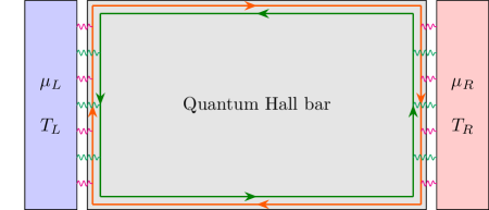
Figure 1: Quantum Hall bar geometry. Two counter-propagating modes (red and green directed lines) are shown. The wiggly lines represent tunnelings from the contacts to the edge modes along left and right line junctions. Interactions between the edge modes are taken to occur along the top and bottom edges.

In order to find the electrical and thermal conductance we assume ideal contacts in the following sense: a mode $\phi_{i}$ ($\phi_{i}^{\prime}$ for the slow modes) carries charge current $I_{i}=\eta_{i}\nu_{i}\sigma_{0}\mu_{c}$ ($I_{i}^{\prime}=\eta_{i}\nu_{i}\sigma_{0}\mu_{c}$) upon leaving the $c\in\{L,R\}$ contact region, while the mode $\tilde{\phi}_{\alpha}$ (refer to (2.2)) carries heat current $\tilde{J}^{Q}_{\alpha}=\eta_{\alpha}c_{\alpha}\kappa_{0}\frac{T^{2}_{c}}{2}$ upon leaving contact $c$.

Given this setup, we use the following procedure to calculate the electrical and thermal conductances of the edge modes. In order to solve for the electrical conductance, we first solve the linear differential equations in (2.8). Taking $\bm{\mathcal{I}}_{n}$ to be the eigenvectors of the matrix $G^{e}$ with eigenvalue $\mathfrak{g}_{n}$, the general solution to the charge transport equations is

$$\bm{I}(x)=\sum_{n}a_{n}\bm{\mathcal{I}}_{n}\operatorname{e}^{\mathfrak{g}_{n}x}$$ (2.20)

for arbitrary coefficients $a_{n}$. We then impose the above “ideal contact” boundary conditions to determine the $a_{n}$ for the top/bottom edges of the Hall bar. We use a similar procedure to solve the heat transport equations (2.11). From these solutions we find the total charge and heat currents moving along the top/bottom edge of the Hall bar:

$$I_{\text{total, top/bottom}} =\sum_{i}I_{i}(x),$$ (2.21a)

$$J^{Q}_{\text{total, top/bottom}} =\sum_{\alpha}\tilde{J}^{Q}_{\alpha}(x),$$ (2.21b)

where $x$ is restricted to either the top/bottom edge of the Hall bar. In the case where some of the modes are strongly mixed (for example the edge modes of the $\nu=2$ quantum Hall state near the $\Delta_{12}=1$ fixed point, as described in section 2.2) we use the slow modes basis to write

$$I_{\text{total, top/bottom}} =\sum_{i\notin\text{strongly mixed}}I_{i}(x)+\sum_{i\in\text{strongly mixed}}I_{i}^{\prime}(x).$$ (2.22)

Note that this expression still represents the total charge current, since the gauge transformations that eliminate the strong-disorder tunnelings (See appendix A) only rotate the neutral currents.

The two-terminal charge and heat Hall conductances are then:

$$G=\frac{I_{\text{total, top}}+I_{\text{total, bottom}}}{\mu_{L}-\mu_{R}},\quad K=\frac{J^{Q}_{\text{total, top}}+J^{Q}_{\text{total, bottom}}}{T_{L}-T_{R}}.$$ (2.23)

Depending on the degree of inter-mode equilibration along the top and bottom edges, the two-terminal conductance takes values between the fully-equilibrated and non–equilibrated values. For the electrical conductance, $G_{\text{fully--eq}}=\sigma_{0}\sum_{i}\eta_{i}\nu_{i}$ while $G_{\text{non--eq}}=\sigma_{0}\sum_{i}\nu_{i}$. For the thermal conductance, $K_{\text{fully-eq}}=\kappa_{0}T\sum_{\alpha}\tilde{\eta}_{\alpha}\tilde{c}_{\alpha}=\kappa_{0}T\sum_{i}\eta_{i}c_{i}$ while $K_{\text{non-eq.}}=\kappa_{0}T\sum_{\alpha}\tilde{c}_{\alpha}=\kappa_{0}T\sum_{i}c_{i}$, where $c_{i},c_{\alpha}$ are the central charges of the various edge modes. (A chiral boson has central charge equal to $+1$; a chiral Majorana fermion has central charge equal to $+1/2$.)

3 Low-temperature theories of anti-Pfaffian edge states at $\nu=5/2$

3.1 Setup and assumptions

In the absence of edge reconstruction, the anti-Pfaffian state at $\nu=5/2$ hosts a total of five edge modes (Fig. 2) [4, 5]. The lowest Landau level contributes (1) a spin-up integer mode and (2) a spin-down integer mode, both moving downstream. From the first Landau level we have (3) a downstream spin-up integer mode, (4) an upstream spin-up $\nu=\frac{1}{2}$ bosonic mode, and an upstream Majorana mode $\psi$.

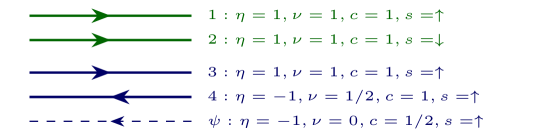
Figure 2: Edge modes of the anti-Pfaffian state at $\nu=5/2$ in the absence of edge reconstruction: $\eta_{i}=\pm 1$ denotes the chirality of the edge mode; $\nu_{i}$ is the charge carried by the edge mode; $c_{i}$ is the central charge of the edge mode; and $s_{i}$ is the spin of the Landau level associated to a particular edge mode. Subscripts labeling the different edge modes are suppressed in the figure.

Charge tunneling between the edge channels requires broken translation symmetry since the edge modes generally lie at different Fermi momenta. Quenched disorder is effective in tunneling electrons only if it can absorb this momentum mismatch. Estimates based on experimental parameters (see [30]) suggest that disorder satisfies this requirement. We take the disorder to be short-ranged. Relaxation of such an assumption, however, has interesting consequences for the equilibration of edge modes, as suggested by Simon [26].

With these considerations, the low-energy effective theory for the anti-Pfaffian edge state at $\nu=5/2$ takes the form $S=\sum_{i=1}^{4}S_{i}+S_{\psi}+\sum_{i\neq j}S_{ij}+S_{\text{tunneling}}$ [4, 5]:

$$S_{i} =-\frac{1}{4\pi}\int_{t,x}\left[\partial_{x}\phi_{i}({\eta_{i}\over\nu_{i}}\partial_{t}\phi_{i}+v_{i}\partial_{x}\phi_{i})\right],$$ (3.1a)

$$S_{\psi} =\frac{1}{4}\int_{t,x}\ i\psi(\partial_{t}\psi-u\partial_{x}\psi),$$ (3.1b)

$$\sum_{i\neq j}S_{ij} =-\sum_{i\neq j}\frac{v_{ij}}{4\pi}\int_{t,x}\ \partial_{x}\phi_{i}\partial_{x}\phi_{j},$$ (3.1c)

$$S_{\text{tunneling}} =-\int_{t,x}\sum_{p\in P}\left[\xi_{p}(x)\operatorname{e}^{i\sum_{j}m^{(p)}_{j}\phi_{j}}\psi^{m^{(p)}_{\psi}}+\text{h.c.}\right].$$ (3.1d)

Similar to before, $P$ is the set of charge-conserving processes defined by the integers $(m_{j}^{(p)},m_{\psi}^{(p)})$ that tunnel electrons between the edge modes, and $\xi_{p}$ is a Gaussian random field with statistical average $\overline{\xi_{p}(x)\xi^{*}_{p^{\prime}}(x^{\prime})}=\delta_{pp^{\prime}}W_{p}\delta(x-x^{\prime})$.

Unless the Coulomb interaction between edge modes of the different Landau levels can be ignored, it’s not obvious what tunneling operators are most relevant. In principle, multi-electron tunneling operators can be more relevant than those that only involve a single-electron tunneling process. However, the largeness of the Landau-gap compared to the electrochemical potential difference between the edge modes, present in the experiments [20, 45], and the large equilibration lengths reported for modes in different Landau levels [42, 46] suggest that tunneling between edge channels belonging to different Landau levels is generally suppressed.

Experiments also report a large equilibration length between spin-up and spin-down modes [41, 46]. This has been attributed to suppressed tunneling between these modes due to weak spin-orbit coupling. This is the assumption made in Ref. [31]; we relax this assumption in this paper. Following the analysis in Section 2.2, where we provided an alternative explanation for the large equilibration length between spin-up and spin-down integer modes, we assume strong tunneling between spin-up and spin-down electrons of the lowest Landau level. Therefore, the most relevant tunnelings to include in $S_{\text{tunneling}}$ are

$$S_{\text{tunneling},12} =-\int_{t,x}\left[\xi_{12}(x)\operatorname{e}^{i(\phi_{1}-\phi_{2})}+\text{h.c.}\right],$$ (3.2a)

$$S_{\text{tunneling},34\psi} =-\int_{t,x}\left[\xi_{34}(x)\operatorname{e}^{i(\phi_{3}+2\phi_{4})}\psi+\text{h.c.}\right].$$ (3.2b)

If the Coulomb interaction between edge modes of different Landau levels is ignored the term $S_{\text{tunneling},12}$ is always relevant; $S_{\text{tunneling},34\psi}$ is relevant if the Coulomb interaction between edge modes of the first Landau level interaction is sufficiently strong. If the modes in the lowest Landau level are decoupled from the modes in the first Landau level (and if equilibration of the first Landau level edge modes occurs via $S_{\text{tunneling},34\psi}$), the low-temperature thermal Hall conductance is the sum of the contributions from the lowest Landau level and the first Landau level $K=K_{\text{LLL}}+K_{\text{1LL}}=\frac{5}{2}\kappa_{0}T$.

However, we aren’t aware of any reason that the Coulomb interaction between the Landau levels is suppressed. Consequently, either of the two tunneling terms in 3.2 can be relevant or irrelevant, depending on the specific nature of the Coulomb interaction, i.e., the values of the $v_{ij}$ in Eq. (3.1c); even strong Coulomb repulsion between all the modes doesn’t uniquely specify an IR fixed point. We identify four possible IR fixed points:

1. $W_{12}=0$ and $W_{34}=0$ while $\Delta_{12}>\frac{3}{2}$ and $\Delta_{34}>\frac{3}{2}$

2. $W_{12}=0$ ($\Delta_{12}>\frac{3}{2}$) and $\Delta_{34}=1$

3. $\Delta_{12}=1$ and $W_{34}=0$ ($\Delta_{34}>\frac{3}{2}$)

4. $\Delta_{12}=1$ and $\Delta_{34}=1.$

Above, $\Delta_{12}$ and $\Delta_{34}$ are the scaling dimensions of $\operatorname{e}^{i(\phi_{1}-\phi_{2})}$ and $\operatorname{e}^{i(\phi_{3}+2\phi_{4})}\psi$. The second case was analyzed in [31], where it was argued that $K=2.5\kappa_{0}T$ requires fine-tuning. The first case is similar to the second one in this regard so we won’t discuss it. In this paper, we investigate the third and the fourth low-temperature fixed points. In Section 4, we describe the conditions under which $K=2.5\kappa_{0}T$ is consistent with either of these fixed points.

3.2 $\Delta_{12}=1,W_{34}=0$ disordered fixed point

In order to study this fixed point we change variables to charge $\phi_{\rho_{\tiny{12}}}=\frac{1}{\sqrt{2}}(\phi_{1}+\phi_{2})$ and spin $\phi_{\sigma_{12}}=\frac{1}{\sqrt{2}}(\phi_{1}-\phi_{2})$ modes [37]. For $v_{ij}$ such that there is no coupling between $\partial_{x}\phi_{\sigma_{12}}$ and $\partial_{x}\phi_{4}$ the theory has an emergent $SO(3)$ symmetry [47, 37, 48] that acts on the $\phi_{\sigma_{12}}$ sector. In Appendix A we show how this symmetry can be used to eliminate $S_{\text{tunneling},12}$, after which an $SO(3)$ transformed spin mode $\tilde{\phi}_{12}$ is introduced. The resulting action becomes $S=S_{\Delta_{12}=1}+S_{\text{int}}$ where

$$S_{\Delta_{12}=1} =S_{\rho_{12}}+S_{\sigma_{12}}+S_{3}+S_{4}+S_{\psi}+\sum_{i\neq j\in\{\rho_{12},3,4\}}S_{ij},$$ (3.3a)

$$S_{\rho_{12}} =-\frac{1}{4\pi}\int_{t,x}\left[\partial_{x}\phi_{\rho_{12}}(\partial_{t}\phi_{\rho_{12}}+v_{\rho_{12}}\partial_{x}\phi_{\rho_{12}})\right],$$ (3.3b)

$$S_{\sigma_{12}} =-\frac{1}{4\pi}\int_{t,x}\left[\partial_{x}\tilde{\phi}_{\sigma_{12}}(\partial_{t}\tilde{\phi}_{\sigma_{12}}+v_{\sigma_{12}}\partial_{x}\tilde{\phi}_{\sigma_{12}}\right],$$ (3.3c)

and

$$S_{\text{int}} =\sum_{i\in\{3,4,\rho_{12}\}}S_{\sigma_{12},i}+S_{\text{tunneling},34\psi},$$ (3.4a)

$$S_{\sigma_{12},i} =-\frac{2v_{\sigma_{12},i}}{4\pi}\int_{t,x}\ \partial_{x}\phi_{i}\left(\frac{\sqrt{2}}{a}O^{zx}\cos(\sqrt{2}\tilde{\phi}_{\sigma_{12}})+\frac{\sqrt{2}}{a}O^{zy}\sin(\sqrt{2}\tilde{\phi}_{\sigma_{12}})+O^{zz}\partial_{x}\tilde{\phi}_{\sigma_{12}}\right).$$ (3.4b)

$O^{ab}(x)$ are matrix elements of the $SO(3)$ rotation that we use to eliminate the $\xi_{12}(x)$ tunneling term. The $S_{ij}$ and $v_{ij}$ with $i,j\in\{\rho_{12},\sigma_{12},3,4\}$ obtain from the $S_{ij}$ and $v_{ij}$ with $i,j\in\{1,2,3,4\}$ after the above field redefinition. $S_{\Delta_{12}=1}$ describes the $\Delta_{12}=1$ fixed point at which the terms in $S_{\text{int}}$ vanish: $v_{\sigma_{12},\rho_{12}}=v_{\sigma_{12},3}=v_{\sigma_{12},4}=W_{34}=0$. The density-density interactions in $S_{\sigma_{12},i}$ are irrelevant near the $\Delta_{12}=1$ fixed point. We assume $S_{\text{tunneling},34\psi}$ is irrelevant at this fixed point, i.e. $\Delta_{34}>\frac{3}{2}$, so that $S_{\Delta_{12}=1}$ describes the low energy behavior of the anti-Pfaffian edge. When $S_{\text{tunneling},34\psi}$ is relevant, the low-energy theory might be described by one of the other fixed points in 3.1. In Appendix C we discuss the domain of validity of describing the low-temperature physics using perturbation theory around the fixed point action 3.3a.

In order to analyze the finite-temperature transport in the vicinity of the $\Delta_{12}=1$ fixed point, the terms in $S_{\text{int}}$ must be included. Consequently, we need to make a choice for the short-ranged Coulomb interaction $v_{ij}$ and diagonalize $S_{\Delta_{12}=1}$. The choice of the Coulomb interaction is non-universal.

Denote by $S_{B}=\sum_{i}S_{i}+\sum_{i\neq j}S_{ij}$, the quadratic part of (3.1) that describes the chiral bosons, and write it as

$$S_{B} =-\frac{1}{4\pi}\int_{t,x}\left[\sum_{i}\frac{\eta_{i}}{\nu_{i}}\partial_{x}\phi_{i}\partial_{t}\phi_{i}+\sum_{i,j}V_{ij}\partial_{x}\phi_{i}\partial_{x}\phi_{j}\right].$$ (3.5)

We model the “velocity matrix” $V_{ij}$ following [49]. In the absence of a short-ranged Coulomb interaction, the action for the bosonic modes is

$$S_{0,B} =-\frac{1}{4\pi}\sum_{i}\int_{t,x}\frac{1}{\nu_{i}}\left[\partial_{x}\phi_{i}(\eta_{i}\partial_{t}\phi_{i}+v^{(0)}_{i}\partial_{x}\phi_{i})\right].$$ (3.6)

Thus, $v^{(0)}_{i}$ is the velocity of $\phi_{i}$ when the Coulomb interaction is ignored. We include the short-ranged Coulomb interaction via the ansatz,

$$S_{\text{Coulomb}}=-\pi w\int_{t,x}\ n_{\text{tot}}(x)^{2}=-\frac{w}{4\pi}\int_{t,x}\ (\sum_{i}\partial_{x}\phi_{i})^{2},$$ (3.7)

where $n_{\text{tot}}=\frac{1}{2\pi}\sum_{i}\partial_{x}\phi_{i}$ is the total charge density and $w$ is the strength of the Coulomb interaction. The Hamiltonian for the bosonic modes is $H_{B}=H_{0,B}+H_{\text{Coulomb}}=\frac{1}{4\pi}\int\mathrm{d}x\sum_{ij}V_{ij}\partial_{x}\phi_{i}\partial_{x}\phi_{j}$, where the “velocity matrix” is

$$V_{ij}=\begin{cases}\frac{1}{\nu_{i}}v^{(0)}_{i}+w\quad&i=j,\\ w&i\neq j.\end{cases}$$ (3.8)

First consider the limit $v_{i}^{(0)}=0$ for all $i$ at which the total Hamiltonian is given by the Coulomb term only. Here, the action is diagonalized using a charge-neutral basis. One such basis choice, that is consistent with our earlier treatment of the relevant $\operatorname{e}^{i(\phi_{1}-\phi_{2})}$ term, is

$$\begin{pmatrix}\phi_{\rho}\\ \phi_{\sigma_{1}}\\ \phi_{\sigma_{2}}\\ \phi_{\sigma_{3}}\end{pmatrix}=\begin{pmatrix}\sqrt{\frac{2}{5}}&\sqrt{\frac{2}{5}}&\sqrt{\frac{2}{5}}&\sqrt{\frac{2}{5}}\\ \frac{1}{\sqrt{2}}&-\frac{1}{\sqrt{2}}&0&0\\ \frac{1}{\sqrt{6}}&\frac{1}{\sqrt{6}}&-\frac{2}{\sqrt{6}}&0\\ \frac{1}{\sqrt{15}}&\frac{1}{\sqrt{15}}&\frac{1}{\sqrt{15}}&\frac{6}{\sqrt{15}}\end{pmatrix}\begin{pmatrix}\phi_{1}\\ \phi_{2}\\ \phi_{3}\\ \phi_{4}\end{pmatrix}.$$ (3.9)

Notice that $\phi_{\sigma_{1}}=\phi_{\sigma_{12}}$. When $v_{i}^{(0)}=0$, the velocity of the charge mode $\phi_{\rho}$ is $\nu w$ ($\nu=\frac{5}{2}$), while the velocities of the neutral modes $\phi_{\sigma_{\alpha}}$ are zero. This three-fold degeneracy in the velocity matrix exists because there is a freedom in choosing the neutral basis given by $\phi_{\sigma_{i}}=\Lambda^{\sigma}_{ij}\phi_{\tilde{\sigma}_{j}}$ where $\Lambda^{\sigma}$ is an arbitrary $SO(2,1)$ rotation.

Experiments [43, 44] suggest the velocity of the charge mode is generally about an order of magnitude larger than the velocity of a neutral mode. This was predicted earlier in [50]. Thus, we assume small, but finite $v^{(0)}_{i}\ll w$. The modes that diagonalize $S_{\Delta_{12}=1}$ when $v_{i}^{(0)}\neq 0$ are not exactly the charge and neutral basis in Eq. (3.9). We denote the diagonal modes as $\phi_{r},\phi_{\sigma_{12}},\phi_{s_{2}},\phi_{s_{3}}$; in the small $v^{(0)}_{i}$ limit, the $\phi_{r}$ mode is “close” to the total charge mode while $\phi_{s_{2}}$ and $\phi_{s_{3}}$ are “almost neutral” modes. Based on (2.18), we expect all the $v^{(0)}_{i}$ as well as the Majorana velocity $u$, to have the same order of magnitude, which we denote by $v^{(0)}$. Therefore, to leading order in $v^{(0)}/w$, the velocities for the modes $\phi_{r},\phi_{\sigma_{12}},\phi_{s_{2}},\phi_{s_{3}}$ are

$$v_{r}=\nu w+O(v^{(0)}),\quad v_{\beta}=O(v^{(0)})\ \text{for}\ \beta=\sigma_{12},s_{2},s_{3}.$$ (3.10)

The density-density interactions between the $\phi_{\sigma_{12}}$ mode and the other modes (the first term in (3.4a)) become irrelevant on scales larger than $v_{\sigma_{12}}^{2}/W_{12}$. In Section 4 we include the effects of such interactions on charge and heat transport near the $\Delta_{12}=1$ fixed point. The couplings for these interactions, $v_{\sigma_{12},r},v_{\sigma_{12},s_{2}}$, and $v_{\sigma_{12},s_{3}}$, vanish in the limit where there’s a degeneracy between the up and down spin electrons in the lowest Landau level. To see this, consider a general $SO(3,1)$ transformation $\Lambda_{i\alpha}$ from the fractional modes $\phi_{i},i=1,2,3,4$ to some new modes $\phi_{\alpha}$ with $\alpha=\sigma_{12},\tilde{2},\tilde{3},\tilde{4}$, such that one of the modes is the spin mode $\phi_{\sigma_{12}}$. From the definition of the spin mode we see that

$$\phi_{1} =\frac{1}{\sqrt{2}}\phi_{\sigma_{12}}+\sum_{\alpha\neq\sigma_{12}}\Lambda_{1\alpha}\phi_{\alpha}$$ (3.11a)

$$\phi_{2} =-\frac{1}{\sqrt{2}}\phi_{\sigma_{12}}+\sum_{\alpha\neq\sigma_{12}}\Lambda_{2\alpha}\phi_{\alpha}$$ (3.11b)

with $\Lambda_{1\alpha}=\Lambda_{2\alpha}$ for $\alpha\neq\sigma_{12}$ while $\Lambda_{3,\sigma_{12}}=\Lambda_{4,\sigma_{12}}=0$. The velocity matrix tranforms as $v_{\alpha\beta}=\sum_{ij}V_{ij}\Lambda_{i\alpha}\Lambda_{j\beta}$. So for $v_{\sigma_{12},\alpha}$ we have

$$\beta\neq\sigma_{12}:v_{\sigma_{12},\beta}= \sum_{ij}V_{ij}\Lambda_{i\sigma_{12}}\Lambda_{j\beta}$$ (3.12)

$$= V_{11}\Lambda_{1,\sigma_{12}}\Lambda_{1,\beta}+V_{22}\Lambda_{2,\sigma_{12}}\Lambda_{2,\beta}+V_{12}\left(\Lambda_{1,\sigma_{12}}\Lambda_{2,\beta}+\Lambda_{2,\sigma_{12}}\Lambda_{1,\beta}\right)$$

$$+\sum_{j\neq 1,2}V_{1j}(\Lambda_{1,\sigma_{12}}\Lambda_{j,\beta}+\Lambda_{j,\sigma_{12}}\Lambda_{1,\beta})+V_{2j}(\Lambda_{2,\sigma_{12}}\Lambda_{j,\beta}+\Lambda_{j,\sigma_{12}}\Lambda_{2,\beta})$$

$$+\sum_{i,j\neq 1,2}V_{ij}\Lambda_{i,\sigma_{12}}\Lambda_{j,\beta}.$$

Using (3.11) we get

$$\beta\neq\sigma_{12}:v_{\sigma_{12},\beta}= \frac{1}{\sqrt{2}}\Lambda_{1,\beta}(V_{11}-V_{22})+\frac{1}{\sqrt{2}}\sum_{j\neq 1,2}\Lambda_{j,\beta}(V_{1j}-V_{2j})$$ (3.13)

which vanishes when $V_{11}=V_{22}$ and $V_{1i}=V_{2i},i=3,4$, i.e., when there exists symmetry between the spin-up and spin-down modes. Note that this result is independent of our specific modeling of the velocity matrix.

3.3 $\Delta_{12}=\Delta_{34}=1$ disordered fixed point

Here, in addition to the field redefinition of the edge modes arising from the lowest Landau level considered in the previous section, we introduce the charge $\phi_{\rho_{34}}=\sqrt{2}(\phi_{3}+\phi_{4})$ and neutral $\phi_{\sigma_{34}}=\phi_{3}+2\phi_{4}$ fields [4, 5]. We also define the Majorana vector $\bm{\psi}^{T}=(\psi_{1},\psi_{2},\psi_{3})$ with Majorana fermions $\psi_{1}=\operatorname{e}^{i\phi_{\sigma_{34}}}+\operatorname{e}^{-i\phi_{\sigma_{34}}},\psi_{2}=i(\operatorname{e}^{i\phi_{\sigma_{34}}}-\operatorname{e}^{-i\phi_{\sigma_{34}}}),\psi_{3}=\psi$. In terms of these fields the action is

$$S =\sum_{i\in\{\sigma_{12},\rho_{12},\rho_{34}\}}S_{i}+\sum_{i\neq j\in\{\sigma_{12},\rho_{12},\sigma_{34},\rho_{34}\}}S_{ij}+S_{\text{neutral}},$$ (3.14a)

$$S_{\rho_{34}} =-\frac{1}{4\pi}\int_{t,x}\ \partial_{x}\phi_{\rho_{34}}(\partial_{t}\phi_{\rho_{34}}+v_{\rho_{34}}\partial_{x}\phi_{\rho_{34}}),$$ (3.14b)

$$S_{\text{neutral}} =S_{\text{sym}}+S_{\text{anis}},$$ (3.14c)

$$S_{\text{sym.}} =\frac{1}{4}\int_{t,x}\ i\bm{\psi}^{T}(\partial_{t}\bm{\psi}-\overline{v}\partial_{x}\bm{\psi}-\frac{\bm{\xi}_{34}.\bm{L}}{2}\bm{\psi}),\quad\bm{\xi}_{34}=\Big{(}\frac{\xi_{34}+\xi_{34}^{*}}{2},\frac{\xi_{34}-\xi_{34}^{*}}{2i},0\Big{)},$$ (3.14d)

$$S_{\text{anis.}} =-\frac{1}{4}\int_{t,x}\ i\bm{\psi}^{T}\delta v\partial_{x}\bm{\psi},$$ (3.14e)

$$S_{ij} =-\frac{2v_{ij}}{4\pi}\int_{t,x}\ \partial_{x}\phi_{i}\partial_{x}\phi_{j},$$ (3.14f)

where the average velocity $\overline{v}\equiv\frac{2v_{\sigma_{34}}+u}{3}$ and the anisotropic velocity matrix $\delta v\equiv\operatorname{diag}(v_{\sigma_{34}}-\overline{v},v_{\sigma_{34}}-\overline{v},u-\overline{v})$. $\bm{L}=(L^{x},L^{y},L^{z})$ is the vector composed of the three generators of $SO(3)$. $S_{\text{sym}}$ has an $SO(3)$ gauge symmetry $\bm{\psi}(x,t)=O(x)\tilde{\bm{\psi}}(x,t)$ provided the disorder vector also transforms as

$$\tilde{\xi}_{34}^{a}=\frac{1}{2}\epsilon^{abc}\left(O^{T}(\bm{\xi}_{34}.\bm{L})O\right)^{bc}+\overline{v}\epsilon^{abc}(O^{T}\partial_{x}O)^{bc}.$$ (3.15)

However under this transformation, the term $\tilde{\bm{\psi}}^{T}(O^{T}\delta v\partial_{x}O)\tilde{\bm{\psi}}$ shows up in $S_{\text{anis}}$. In order to get rid of such a term we instead require $\xi_{34}$ to transform as

$$\tilde{\xi}_{34}^{a}=\frac{1}{2}\epsilon^{abc}\left(O^{T}(\bm{\xi}_{34}.\bm{L})O\right)^{bc}+\epsilon^{abc}(O^{T}v\partial_{x}O)^{bc},$$ (3.16)

with velocity matrix $v=\operatorname{diag}(v_{\sigma_{34}},v_{\sigma_{34}},u)$. Requiring $\tilde{\bm{\xi}}_{34}=0$, the transformed action becomes $S=S_{\Delta_{12}=\Delta_{34}=1}+S_{\text{int}}$ where

$$S_{\Delta_{12}=\Delta_{34}=1} =\sum_{i\in\{\sigma_{12},\rho_{12},\rho_{34}\}}S_{i}+S_{\text{neutral sym}}+S_{\rho_{12},\rho_{34}},$$ (3.17a)

$$S_{\text{neutral sym}} =\frac{1}{4}\int_{t,x}\ i\tilde{\bm{\psi}}^{T}(\partial_{t}\tilde{\bm{\psi}}-\overline{v}\partial_{x}\tilde{\bm{\psi}}),$$ (3.17b)

$$S_{\rho_{12},\rho_{34}} =-\frac{v_{\rho_{12},\rho_{34}}}{8\pi}\int_{t,x}\ \partial_{x}\phi_{\rho_{12}}\partial_{x}\phi_{\rho_{34}},$$ (3.17c)

and

$$S_{\text{int}} =\sum_{i\in\{\rho_{12},\rho_{34}\}}(S_{\sigma_{34},i}+S_{\sigma_{12},i})+S_{\sigma_{12},\sigma_{34}}+S_{\text{neutral int}},$$ (3.18a)

$$S_{\text{neutral int}} =-\int_{t,x}\ i\tilde{\bm{\psi}}^{T}\widetilde{\delta v}\partial_{x}\tilde{\bm{\psi}},$$ (3.18b)

$$S_{\sigma_{34},i} =-\frac{v_{i.\sigma_{34}}}{8\pi}\int_{t,x}\ \partial_{x}\phi_{\sigma_{34}}\left(i\tilde{\bm{\psi}}^{T}L^{z}(x)\tilde{\bm{\psi}}\right),$$ (3.18c)

$$S_{\sigma_{12},\sigma_{34}} =-\frac{2v_{\sigma_{12},\sigma_{34}}}{4\pi}\int_{t,x}\left(i\tilde{\bm{\psi}}^{T}L^{z}(x)\tilde{\bm{\psi}}\right)$$ (3.18d)

$$\qquad\qquad\times\left(\frac{\sqrt{2}}{a}O^{zx}\cos(\sqrt{2}\tilde{\phi}_{\sigma_{12}})+\frac{\sqrt{2}}{a}O^{zy}\sin(\sqrt{2}\tilde{\phi}_{\sigma_{12}})+O^{zz}\partial_{x}\tilde{\phi}_{\sigma_{12}}\right),$$

with $\widetilde{\delta v}(x)\equiv O^{T}(x)\delta vO(x)$ and $L^{z}(x)\equiv O^{T}(x)L^{z}O(x)$. The $\Delta_{12}=\Delta_{34}=1$ fixed point is described by $S_{\Delta_{12}=\Delta_{34}=1}$ about which the terms in $S_{\sigma_{34},i}$ and $S_{\sigma_{34},i}$ are irrelevant. Here, the auto-correlation of elements of matrices $L^{z}(x)$ and $\widetilde{\delta v}(x)$ decay on length scales $\sim\overline{v}^{2}/W_{34}$.

We model the short-ranged Coulomb interaction as in the previous section. Here, the diagonal modes are $\phi_{r},\phi_{\sigma_{12}},\phi_{s_{2}},\phi_{\sigma_{34}}$, where $\phi_{s_{2}}$ is some “almost neutral” mode. To leading order in $v^{(0)}/w$ the velocities for these modes are

$$v_{r}=\nu w+O(v^{(0)}),\quad v_{\beta}=O(v^{(0)})\ \text{for}\ \beta=\sigma_{12},s_{2},\sigma_{34}.$$ (3.19)

Since $u=O(v^{(0)})$, we can write $\overline{v}\approx O(v^{(0)})$. As for the magnitude of couplings in (3.18), we have $v_{\sigma_{34},\beta}=O(v^{(0)})$ for $\beta=r,s_{2}$ while $v_{\sigma_{12},\beta}$ vanish for $\beta=r,\sigma_{12},s_{2}$ in the spin-degenerate limit as demonstrated in the previous section.

4 Transport and equilibration along the $\nu=5/2$ edge

In this section, we analyze the low-temperature transport properties of the effective theories of the $\nu=5/2$ anti-Pfaffian state described in Sections 3.2 and 3.3. We will apply charge and heat kinetic equations introduced in Section 2 to each of these fixed points, calculate the expressions for conductivity coefficients, and eventually solve for the electrical and thermal Hall conductances. We estimate the parameter regime that describes the experimental observation of $\kappa=2.5\kappa_{0}T$ so as to determine the experimental relevance of each fixed point.

4.1 $\Delta_{12}=1$ fixed point

4.1.1 Charge transport

At this fixed point, the processes that cause equilibration are the irrelevant terms in (3.4a). Using (2.8) (see appendix B.1 for details) we write down the equations describing charge transport resulting from such interactions. In the basis $(I^{\prime}_{1},I^{\prime}_{2},I_{3},I_{4})$ the matrix $G^{e}$ is

$$G^{e} =-(\sum_{\beta=r,s_{2},s_{3}}g_{V_{\sigma_{12},\beta}})\begin{pmatrix}1&-1&0&0\\ -1&1&0&0\\ 0&0&0&0\\ 0&0&0&0\end{pmatrix}-g_{V_{34}}\begin{pmatrix}0&0&0&0\\ 0&0&0&0\\ 0&0&1&2\\ 0&0&-1&-2\end{pmatrix}$$ (4.1)

with

$$\beta=r,s_{2},s_{3}:g_{V_{\sigma_{12},\beta}} =\frac{2\pi^{2}v_{\sigma_{12},\beta}^{2}T^{2}}{3v_{\beta}^{2}W_{12}}$$ (4.2a)

$$g_{V_{34}} =\frac{\Gamma(\Delta_{34})^{2}}{\Gamma(2\Delta_{34})}\frac{W_{34}}{\overline{v}_{V_{34}}^{2\Delta_{34}}}\left(2\pi aT\right)^{2\Delta_{34}-2},\quad\overline{v}_{V_{34}}=O(v^{(0)}).$$ (4.2b)

The velocities are defined in (3.10), and $a$ is the short-distance cutoff [39].

The last term in $G^{e}$ couples the downstream and upstream charge modes. Therefore largeness of $g_{V_{34}}$ (see below) is required for the proper quantization of the electrical conductance at $G=2.5\sigma_{0}$. To quantify this we solve for the electrical conductance using (4.1) and boundary conditions specified in Section 2.3. We find

$$G=\sigma_{0}\left(2+\frac{2+\operatorname{e}^{-g_{V_{34}}L}}{2(2-\operatorname{e}^{-g_{V_{34}}L})}\right),$$ (4.3)

where $L$ is the effective length on the sample’s top/bottom edge along which equilibration takes place. If the electrical conductance is measured to be $G=2.50\sigma_{0}$ within the uncertainty $\Delta G=0.01\sigma_{0}$ we find the bound $g_{V_{34}}L\gtrsim 4$.

4.1.2 Heat transport

Based on (2.11), the heat transport matrix $G^{Q}$ in the basis $(r,\phi_{\sigma_{12}},\phi_{s_{2}},\phi_{s_{3}},\psi)$ is

$$G^{Q}= \frac{12g_{V_{\sigma_{12},r}}}{5}\begin{pmatrix}-1&1&0&0&0\\ 1&-1&0&0&0\\ 0&0&0&0&0\\ 0&0&0&0&0\\ 0&0&0&0&0\end{pmatrix}+\frac{12g_{V_{\sigma_{12},s_{2}}}}{5}\begin{pmatrix}0&0&0&0&0\\ 0&-1&1&0&0\\ 0&1&-1&0&0\\ 0&0&0&0&0\\ 0&0&0&0&0\end{pmatrix}+\frac{12g_{V_{\sigma_{12},s_{3}}}}{5}\begin{pmatrix}0&0&0&0&0\\ 0&-1&0&-1&0\\ 0&0&0&0&0\\ 0&1&0&1&0\\ 0&0&0&0&0\end{pmatrix}+\frac{12g_{V_{34}}}{1+2\Delta_{34}}$$ (4.4)

$$\times\begin{pmatrix}-d_{r}(d_{s_{2}}+d_{s_{3}}+d_{\psi})&0&d_{r}d_{s_{2}}&-d_{r}d_{s_{3}}&-2d_{r}d_{\psi}\\ 0&0&0&0&0\\ d_{r}d_{s_{2}}&0&-d_{s_{2}}(d_{r}+d_{s_{3}}+d_{\psi})&-d_{s_{2}}d_{s_{3}}&-2d_{s_{2}}d_{\psi}\\ d_{r}d_{s_{3}}&0&d_{s_{2}}d_{s_{3}}&d_{s_{3}}(d_{r}+d_{s_{2}}+d_{\psi})&-2d_{s_{3}}d_{\psi}\\ d_{r}d_{\psi}&0&d_{s_{2}}d_{\psi}&-d_{s_{3}}d_{\psi}&2d_{\psi}(d_{r}+d_{s_{2}}+d_{s_{2}})\end{pmatrix}$$ (4.5)

where $d_{\psi}=\frac{1}{2}$ and $d_{\alpha}=\left(\Lambda_{3\alpha}+2\Lambda_{4\alpha}\right)^{2}/2$. Also we have $\sum_{\alpha=r,s_{2},s_{3},\psi}d_{\alpha}=\Delta_{34}$. See B.2 for the definition of $d_{\alpha}$. $\Lambda$ is the $SO(3,1)$ transformation expressing the fractional modes $\phi_{i}$ in terms of $(\phi_{r},\phi_{\sigma_{12}},\phi_{s_{2}},\phi_{s_{3}})$, i.e., the diagonal modes of $S_{\Delta_{12}=1}$.

This transformation depends on the velocity matrix in (3.3a). We use the velocity matrix in Eq. (3.8) in order to estimate the $d_{\alpha}$. In the $v^{(0)}_{i}/w=0$ limit, $\phi_{r}$ is the total charge mode, and, consequently, it commutes with the neutral mode $\phi_{3}+2\phi_{4}$. Therefore, in this limit, $d_{r}=\left(\Lambda_{3,r}+2\Lambda_{4,r}\right)^{2}/2=0$. For finite but small $v^{(0)}/w$, we have $d_{r}=O\left((\frac{v^{(0)}}{w})^{2}\right)$ to leading order.

In order to estimate $d_{s_{2}}$ and $d_{s_{3}}$, we look at the spin of the operator $\operatorname{e}^{i\phi_{3}+2i\phi_{4}}$. Generally, for a set of chiral bosons $\phi_{i}$ with commutation relation $[\phi_{i}(x),\phi_{j}(x^{\prime})]=\pi iK^{-1}_{ij}\operatorname{sign}(x-x^{\prime})$, the spin of the vertex operator $\operatorname{e}^{i\sum_{i}n_{i}\phi_{i}}$ is

$$h_{-}=\frac{1}{2}n_{i}K^{-1}_{ij}n_{j}=\Delta_{R}-\Delta_{L},$$ (4.6)

where $\Delta_{R}$ ($\Delta_{L}$) is the scaling dimension of the right-moving (left-moving) part of $\operatorname{e}^{i\sum_{i}n_{i}\phi_{i}}$. Therefore, the spin of the tunneling operator $\operatorname{e}^{i\phi_{3}+2i\phi_{4}}$ is $h_{-}=-\frac{1}{2}=\Delta_{R}-\Delta_{L}$. Also, we have $\Delta_{R}=d_{r}+d_{s_{2}}$ and $\Delta_{L}=d_{s_{3}}$. Along with $d_{r}+d_{s_{2}}+d_{s_{3}}+d_{\psi}=\Delta_{34}$, to leading order in $v^{(0)}_{i}/w$ we find

$$d_{s_{2}} =\frac{\Delta_{34}-1}{2}-d_{r}=\frac{\Delta_{34}-1}{2}-O\left((\frac{v^{(0)}}{w})^{2}\right)$$ (4.7a)

$$d_{s_{3}} =\frac{\Delta_{34}}{2}.$$ (4.7b)

As we mentioned in Section 3.2, we take $\Delta_{34}\geq\frac{3}{2}$ so that $S_{\Delta_{12}}=1$ describes the low-energy physics of the $\Delta_{12}=1$ fixed point. On the other hand, since $g_{V_{34}}L$ is large, based on Eq. (4.2), we don’t expect $\Delta_{34}$ to be very large. This is due to the fact that i) the pre-factor $\Gamma(\Delta_{34})^{2}/\Gamma(2\Delta_{34})$ vanishes rapidly for large $\Delta_{34}$ and ii) $g_{V_{34}}\sim T^{2(\Delta_{34}-1)}$ and so the equilibration process corresponding to $g_{V_{34}}$ would have sub-leading contribution at small temperatures, if $\Delta_{34}$ was large.

We can estimate $\Delta_{34}$ for $v^{(0)}_{i}=v^{(0)}$. In this case, using (3.9) we can write

$$H =\frac{1}{4\pi}\int_{x}V_{ij}\partial_{x}\phi_{i}\partial_{x}\phi_{j}$$

$$=\frac{1}{4\pi}\int_{x}\Big{[}(w+\frac{7}{5}v^{(0)})(\partial_{x}\phi_{\rho})^{2}+v^{(0)}(\partial_{x}\phi_{\sigma_{1}})^{2}$$ (4.8)

$$\qquad\qquad\qquad+v^{(0)}(\partial_{x}\phi_{\sigma_{2}})^{2}+\frac{7}{5}v^{(0)}(\partial_{x}\phi_{\sigma_{3}})^{2}-\frac{4\sqrt{6}}{5}v^{(0)}\partial_{x}\phi_{\rho}\partial_{x}\phi_{\sigma_{3}}\Big{]}.$$

Therefore, for small $v^{(0)}/w$ a small rotation in the $(\phi_{\rho},\phi_{\sigma_{3}})$ plane would diagonalize the Hamiltonian. So, using (3.9) we find $\Delta_{34}=\frac{5}{3}$ in the vanishing $v^{(0)}/w$ limit.

We are interested in determining the regime for which this matrix $G^{Q}$ leads to a thermal Hall conductance $K=2.5\kappa_{0}T$ within the uncertainties of the experiment. Quantization of electrical conductance $G=2.5\sigma_{0}$ implies that $g_{V_{23}}$ is large. Looking at the last term in (4.4), more specifically, the $(\phi_{s_{2}},\phi_{s_{3}},\psi)$ block, it appears that the $\phi_{s_{2}}$,$\phi_{s_{3}}$ and $\psi$ modes equilibrate with each other. For the moment, let’s assume they are completely equilibrated; we will relax this assumption later. In this case, we can think of these modes as a single upstream mode with central charge $c=\frac{1}{2}$. We call this mode $\tilde{s}$.

If equilibration between the first two modes in (4.4) and the $\tilde{s}$ mode is suppressed, the thermal conductance theis sum of the contributions from the first two modes $K_{r+\sigma_{12}}$ and from the $\tilde{s}$ mode $K_{\tilde{s}}$. That is $K=K_{r+\sigma_{12}}+K_{\tilde{s}}=\left(2+\left|-0.5\right|\right)\kappa_{0}T=2.5\kappa_{0}T$. This requires

$$g_{V_{\sigma_{12},s_{2}}}L\ll 1,\quad g_{V_{\sigma_{12},s_{3}}}L\ll 1,\quad g_{r,\tilde{s}}L\ll 1,$$ (4.9)

where we defined $g_{r,\tilde{s}}=d_{r}(\Delta_{34}-d_{r})g_{V_{34}}$. Therefore, we see that there exists a regime of parameters where the fixed point $\Delta_{12}=1$ can be consistent with experiments. Using the details of the experimental measurements, we can gain a more quantitative estimation of this regime.

We use the above $G^{Q}$ matrix and boundary conditions given in Section 2.3 to solve for the thermal conductance. Following our earlier discussion we will take $\Delta_{34}=\frac{5}{3}$, and consequently $d_{s_{2}}=\frac{1}{3},d_{s_{3}}=\frac{5}{6}$. Later, we will discuss how our results depend on these values.

We also ignore the first term in (4.4) in the remainder. This follows from our discussion in Section 2.2: we expect $g_{\sigma_{12},r}L$ to be suppressed both due to the strong Coulomb interaction and small spin gap. Also, since $g_{\sigma_{12},r}$ quantifies equilibration between co-propagating modes, its magnitude does not have much effect on the thermal conductance.

The contour plot of $K(g_{V_{\sigma_{12},s_{2}}}L,g_{V_{\sigma_{12},s_{2}}}L,g_{r,\tilde{s}}L,g_{V_{34}}L)$ along several surfaces is given in Fig. 3. The thermal conductance observed in the experiments ([20]) at temperatures ($T\approx 18\operatorname{-}25\ mK$) $2.49\kappa_{0}T<K<2.57\kappa_{0}T$ is enclosed within the white contours. The hatched region represents the regime where the electrical conductance $G=(2.50\pm 0.01)\sigma_{0}$.

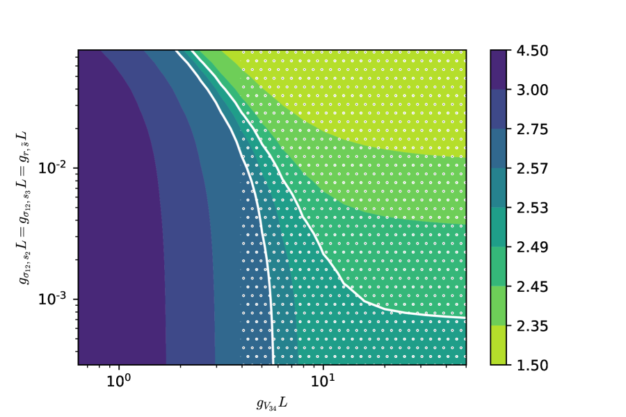
(a) $g_{V_{\sigma_{12},s_{2}}}=g_{V_{\sigma_{12},s_{2}}}=g_{r,\tilde{s}}$

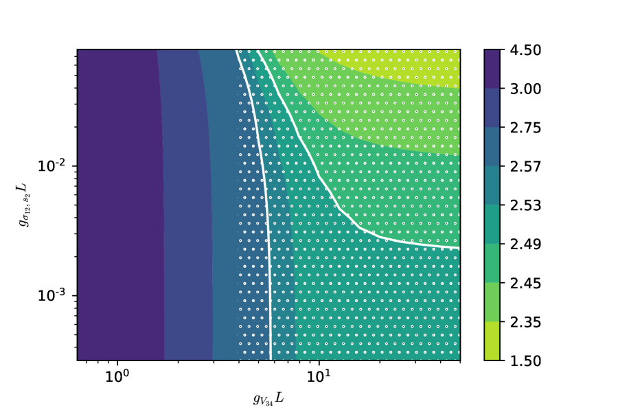
(b) $g_{V_{\sigma_{12},s_{3}}}=g_{r,\tilde{s}}=0$

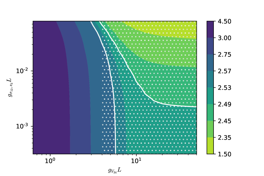
(c) $g_{V_{\sigma_{12},s_{2}}}=g_{r,\tilde{s}}=0$

(d) $g_{V_{\sigma_{12},s_{2}}}=g_{V_{\sigma_{12},s_{3}}}=0$

Figure 3: Contour plot of thermal conductance about the $\Delta_{12}=1$ fixed point, $K(g_{V_{\sigma_{12},s_{2}}}L,g_{V_{\sigma_{12},s_{3}}}L,g_{r,\tilde{s}}L,g_{V_{34}}L)/\kappa_{0}T$ along several surfaces. $\Delta_{34}=5/3$ for all the sub-plots. The regions within the white contour represent the measured thermal conductance $K=(2.53\pm 0.04)\kappa_{0}T$, while the hatched regions represent the regime where $G=(2.50\pm 0.01)\sigma_{0}$.

We observe that not all of the region observed in the experiment $2.49\kappa_{0}T<K<2.75\kappa_{0}T$ is consistent with the electrical conductance $G=(2.50\pm 0.01)\sigma_{0}$: we find that when $K\gtrsim 2.65\kappa_{0}T$, the electrical conductance deviates from $G=(2.50\pm 0.01)\sigma_{0}$. In addition, we can deduce some information about which point of the region $2.49\kappa_{0}T<K<2.75\kappa_{0}T$ we are at by examining how the thermal conductance varies as a function of temperature.

The conductivity coefficients have power law dependence on temperature as Eq. (4.2). Therefore, the thermal conductance moves along straight lines in Fig. 3, as the temperature is varied. From the experimental data, as the temperature is lowered from $T\approx 18\operatorname{-}25\ mK$ to $T\approx 12\ mK$, i.e., by a factor of about $2$, the thermal conductance increases from $K\approx 2.53\kappa_{0}T$ to $K\approx 2.75\kappa_{0}T$. It follows that $g_{34}$ would vary by a factor of $2^{(2\Delta_{34}-2)}$ while $g_{\sigma_{12},s_{2}}$ and $g_{\sigma_{12},s_{3}}$ would vary by a factor of $4$. We can look for lines in the space of conductivity coefficients where such a variation occurs.

First, we look at how the thermal conductance varies along the surface $g_{\sigma_{12},s_{2}}=g_{\sigma_{12},s_{3}}$ when $g_{r,\tilde{s}}=0$. This is demonstrated in Fig. 4. The red line showcases a variation of conductivity coefficients with temperature that is consistent with the experiments: as the temperature is lowered by a factor of $\sim 2$, between the cross marks, the thermal conductance increases from $K\approx 2.53\kappa_{0}T$ to $K\approx 2.75\kappa_{0}T$. This gives us a rough estimate for the value of the conductivity coefficients at these temperatures. Examining the red line in Fig. 4 for $T=18\operatorname{-}25\ mK$, we find

$$g_{V_{34}}L\approx 7,\quad g_{\sigma_{12},s_{2}/s_{3}}L\approx 0.005.$$ (4.10)

A similar picture also shows $g_{r,\tilde{s}}L\approx 0.005$. Here, the thermal conductance does not vary much as a function of $g_{\sigma_{12},s_{2}/s_{3}}$ and $g_{r,\tilde{s}}$ when these coefficients are small. Consequently, the error in the estimate of $g_{\sigma_{12},s_{2}/s_{3}}$ and $g_{r,\tilde{s}}$ is large and the above estimates for $g_{\sigma_{12},s_{2}/s_{3}}$ and $g_{r,\tilde{s}}$ should be interpreted as upper bounds.

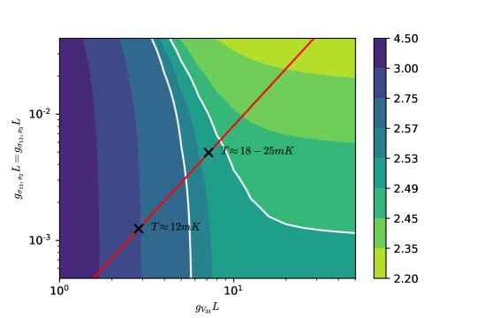
Figure 4: Thermal conductance about the $\Delta_{12}=1$ fixed point on the surface $g_{V_{\sigma_{12},s_{2}}}=g_{V_{\sigma_{12},s_{3}}}$ and $g_{r,\tilde{s}}=0$. $\Delta_{34}=5/3$. The red line represents a typical line along which the thermal conductance varies as a function of temperature. This specific red line passes through points that are consistent with measurements of thermal conductance.

Based on these estimates, we infer

$$\frac{g_{r,\tilde{s}}}{g_{V_{34}}}=(\Delta_{34}-d_{r})d_{r}\sim(\frac{v^{(0)}}{w})^{2}\lesssim 0.001.$$ (4.11)

Since $d_{r}\sim(\frac{v^{(0)}}{w})^{2}$ the above bound is not unexpected for strong short-ranged Coulomb interactions. Our numerical estimates for $d_{r}$ based on the velocity matrix in Eq. 3.8 and sensible choice of $v^{(0)}_{i}$’s, do satisfy this bound for $v^{(0)}_{i}$’s as large as $w/5$.

On the other hand, the coefficients $g_{\sigma_{12},s_{2}}$ and $g_{\sigma_{12},s_{3}}$ in (4.2) are proportional to the square of $v_{\sigma_{12},s_{2}}$ and $v_{\sigma_{12},s_{3}}$. As we demonstrated in Eq. (3.13), these velocity entries vanish in the spin-degenerate limit. Therefore, it is not unexpected that the bound $g_{\sigma_{12},s_{2}/s_{3}}L\lesssim 0.01$ is satisfied when the spin gap is small. However, we don’t have any estimate for these conductivity coefficients based on the experimental data.

In order to find these results, we used the estimate $\Delta_{34}=5/3$. In order to see how much our results depend on this estimate, we look at two other cases: i) $\Delta_{34}=3/2$ and ii) $\Delta_{34}=2$. For these two values, we plot $K(g_{V_{\sigma_{12},s_{2}}}L,g_{V_{\sigma_{12},s_{2}}}L,g_{r,\tilde{s}}L=0,g_{V_{34}}L)$ along the $g_{V_{\sigma_{12},s_{2}}}=g_{V_{\sigma_{12},s_{3}}}$ surface in Fig. 5. First, we see that while the observation of $G=(2.50\pm 0.01)\sigma_{0}$ is mostly consistent with $2.49\kappa_{0}T\leq K\leq 2.75\kappa_{0}T$ for $\Delta_{34}=3/2$, this is not the case for $\Delta_{34}=2$: in the region $2.57\kappa_{0}T\leq K\leq 2.75\kappa_{0}T$, the electrical conductance deviates from $G=(2.50\pm 0.01)\sigma_{0}$.

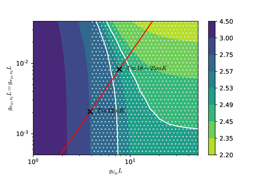
(a) $\Delta_{34}=3/2$

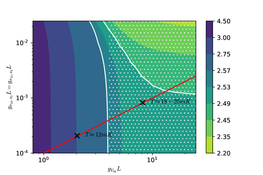
(b) $\Delta_{34}=2$

Figure 5: Contour plot of thermal conductance about the $\Delta_{12}=1$ fixed point, $K(g_{V_{\sigma_{12},s_{2}}}L,g_{V_{\sigma_{12},s_{3}}}L,g_{r,\tilde{s}}L,g_{V_{34}}L)/\kappa_{0}T$ along the surface $g_{V_{\sigma_{12},s_{2}}}=g_{V_{\sigma_{12},s_{2}}},g_{r,\tilde{s}}=0$. The hatched regions represent the regime where $G=(2.50\pm 0.01)\sigma_{0}$.

In addition, while for $\Delta_{34}=3/2$ the bounds on the conductivity coefficients are close to the $\Delta_{34}=5/3$ case, for $\Delta_{34}=2$ we get

$$g_{V_{34}}L\approx 10,\quad g_{\sigma_{12},s_{2}/s_{3}}L\lesssim 0.001,$$ (4.12)

which are much stronger bounds.

We conclude that there exists a regime of parameters about the $\Delta_{12}=1$ fixed point of the anti-Pfaffian edge state where $K\approx 2.5\kappa_{0}T$ is observed in a range of temperatures ($T\approx 18\operatorname{-}25\ mK$). Our estimates demonstrate that this regime is possible for realistic parameters only when $\Delta_{34}\lesssim 5/3$.

4.2 $\Delta_{12}=\Delta_{34}=1$ fixed point

4.2.1 Charge transport

At this fixed point, the processes that cause equilibration are the irrelevant terms in (3.18). To find the kinetic equations involving the second Landau level modes, we first introduce the neutral currents operators

$$J_{34}^{a}\equiv\frac{i}{8\pi}\bm{\psi}^{T}L^{a}\bm{\psi}$$ (4.13)

where $L^{a},a=x,y,z$ are the generators of $SO(3)$. In terms of these operators we have $\frac{1}{2\pi}\partial_{x}\phi_{\sigma_{34}}=J^{z}_{34}$. Using a similar set of calculations as in section B.1.2, we derive the kinetic equation for the gauge-transformed density

$$\tilde{n}_{\sigma_{34}}\equiv\frac{1}{2\pi}\partial_{x}\tilde{\phi}_{\sigma_{34}}\equiv\tilde{J}^{z}_{34}=\frac{i}{8\pi}\bm{\tilde{\psi}}^{T}L^{z}\bm{\tilde{\psi}}.$$ (4.14)

We also define the “slow modes” basis as

$$I_{3}^{\prime} =\sqrt{2}I_{\rho_{34}}-\tilde{I}_{\sigma_{34}}$$ (4.15a)

$$I^{\prime}_{4} =-\frac{1}{\sqrt{2}}I_{\rho_{34}}+\tilde{I}_{\sigma_{34}}$$ (4.15b)

where $I_{\rho_{34}}$ is the charge current carried by the mode $\phi_{\rho_{34}}$ and the current neutral current $\tilde{I}_{\sigma_{34}}$ is defined by the conservation equation

$$\partial_{x}\tilde{I}_{\sigma_{34}}+\partial_{t}\tilde{n}_{\sigma_{34}}=0.$$ (4.16)

It follows that for charge equilibration in the basis $(I^{\prime}_{1},I^{\prime}_{2},I^{\prime}_{3},I^{\prime}_{4})$ we have

$$G^{e} =-(\sum_{\beta=r,s_{2},\sigma_{34}}g_{V_{\sigma_{12},\beta}})\begin{pmatrix}1&-1&0&0\\ -1&1&0&0\\ 0&0&0&0\\ 0&0&0&0\end{pmatrix}-(\sum_{\beta=r,\sigma_{12},s_{2}}g_{V_{\sigma_{34},\beta}})\begin{pmatrix}0&0&0&0\\ 0&0&0&0\\ 0&0&1&2\\ 0&0&-1&-2\end{pmatrix}$$ (4.17)

with

$$g_{V_{\sigma_{12},\sigma_{34}}} =\frac{2\pi^{2}v_{\sigma_{12},\sigma_{34}}^{2}}{3(v_{\sigma_{12}}^{2}W_{34}+v_{\sigma_{34}}^{2}W_{12})}T^{2}$$ (4.18a)

$$\beta=r,s_{2}:g_{V_{\sigma_{12},\beta}} =\frac{2\pi^{2}v_{\sigma_{12},\beta}^{2}}{3v_{\beta}^{2}W_{12}}T^{2}$$ (4.18b)

$$\beta=r,s_{2}:g_{V_{\sigma_{34},\beta}} =\frac{2\pi^{2}v_{\sigma_{34},\beta}^{2}T^{2}}{3v_{\beta}^{2}W_{34}}.$$ (4.18c)

We can calculate the electrical conductance as in the previous section. The solution is similar to Eq. (4.3) with $g_{V_{34}}$ replaced by $\sum_{\beta=r,\sigma_{12},s_{2}}g_{V_{\sigma_{34},\beta}}$. An electrical conductance of $G=(2.50\pm 0.01)\sigma_{0}$ implies $\sum_{\beta=r,\sigma_{12},s_{2}}g_{V_{\sigma_{34},\beta}}L\gtrsim 4$. Looking at Eq. (4.18) we can estimate the relative magnitude of the terms in $\sum_{\beta=r,\sigma_{12},s_{2}}g_{V_{\sigma_{34},\beta}}$. We find

$$\frac{g_{V_{\sigma_{34},r}}}{g_{V_{\sigma_{34},s_{2}}}} =(\frac{v_{\sigma_{34},r}v_{s_{2}}}{v_{\sigma_{34},s_{2}}v_{r}})^{2}\sim(\frac{v^{(0)}}{\nu w})^{2},$$ (4.19a)

$$\frac{g_{V_{\sigma_{34},\sigma_{12}}}}{g_{V_{\sigma_{34},s_{2}}}} \approx\frac{W_{34}}{W_{12}+W_{34}}.(\frac{v_{\sigma_{34},\sigma_{12}}v_{s_{2}}}{v_{\sigma_{34},s_{2}}v_{\sigma_{12}}})^{2}\sim\frac{W_{34}}{W_{12}+W_{34}}.(\frac{v_{\sigma_{34},\sigma_{12}}}{v^{(0)}})^{2}.$$ (4.19b)

Therefore, both $g_{V_{\sigma_{34},\sigma_{12}}}$ and $g_{V_{\sigma_{34},r}}$ are much smaller than $g_{V_{\sigma_{34},s_{2}}}$ for strong Coulomb interactions and small spin gap, and so we have $g_{V_{\sigma_{34},s_{2}}}L\gtrsim 1$ based on quantization of the electrical conductance. In the above we used the estimate that $v_{s_{2}},v_{\sigma_{12}},v_{\sigma_{34},r},v_{\sigma_{34},s_{2}}$ all have the same order of magnitude $v^{(0)}$. Also, based on the velocity matrix of Eq. 3.8 and using Eq. 3.13 we should have $v_{\sigma_{34},\sigma_{12}}=0$. However, since we only take this velocity matrix as an estimation, we allow for finite $v_{\sigma_{34},\sigma_{12}}$ which vanishes in the spin-symmetric limit.

4.2.2 Heat transport

At this fixed point, since there exists an $SO(3)$ symmetry between the three Majorana modes, we take their contribution as one upstream mode with central charge $c=\frac{3}{2}$. We call this mode $\Psi$. Therefore, in the basis $(r,\sigma_{12},s_{2},\Psi)$ we have

$$G^{Q}= \frac{12}{5}g_{V_{\sigma_{12},r}}\begin{pmatrix}-1&1&0&0\\ 1&-1&0&0\\ 0&0&0&0\\ 0&0&0&0\end{pmatrix}+\frac{12}{5}g_{V_{\sigma_{12},s_{2}}}\begin{pmatrix}0&0&0&0\\ 0&-1&1&0\\ 0&1&-1&0\\ 0&0&0&0\end{pmatrix}+\frac{12}{5}g_{V_{\sigma_{12},\sigma_{34}}}\begin{pmatrix}0&0&0&0\\ 0&-1&0&-2/3\\ 0&0&0&0\\ 0&1&0&2/3\end{pmatrix}$$ (4.20)

$$+\frac{12}{5}g_{V_{\sigma_{34},r}}\begin{pmatrix}-1&0&0&-2/3\\ 0&0&0&0\\ 0&0&0&0\\ 1&0&0&2/3\end{pmatrix}+\frac{12}{5}g_{V_{\sigma_{34},s_{2}}}\begin{pmatrix}0&0&0&0\\ 0&0&0&0\\ 0&0&-1&-2/3\\ 0&0&1&2/3\end{pmatrix}.$$

Since $g_{V_{\sigma_{34},s_{2}}}L\gtrsim 1$, the modes $s_{2}$ and $\Psi$ are expected to be well equilibrated. Therefore, similar to the $\Delta_{12}=1$ fixed point, the thermal conductance $K\approx 2.5\kappa_{0}T$ is only possible when equilibration between the modes $\{r,\sigma_{12}\}$ and $\{s_{2},\Psi\}$ is suppressed. In order to look for such a regime, we solve the heat transport equation using the above $G^{Q}$ matrix, and calculate the thermal conductance as a function of $g_{V_{\sigma_{12},s_{2}}},g_{V_{\sigma_{12},\sigma_{34}}},g_{V_{\sigma_{34},r}}$ and $g_{V_{\sigma_{34},r}}$. As before, we ignore the first term in $G^{Q}$. Fig. 6 shows the contour plot of the thermal conductance along the surface $g_{V_{\sigma_{12},s_{2}}}=g_{V_{\sigma_{12},\sigma_{34}}}=g_{V_{\sigma_{34},r}}$. The region within the white contour has $2.49\kappa_{0}T<K<2.57\kappa_{0}T$, while the hatched region has electrical conductance $G=(2.50\pm 0.01)\sigma_{0}$.

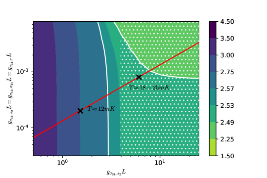
Figure 6: Thermal conductance about the $\Delta_{12}=\Delta_{34}=1$ fixed point, along the surface $g_{V_{\sigma_{12},s_{2}}}=g_{V_{\sigma_{12},\sigma_{34}}}=g_{V_{\sigma_{34},r}}$. The region within the white contour has $2.49\kappa_{0}T<K<2.57\kappa_{0}T$, while the hatched region has electrical conductance $G=(2.50\pm 0.01)\sigma_{0}$. The thermal conductance varies along lines parallel to the red line as the temperature is varied.

Here, unlike the $\Delta_{12}=1$ fixed point, there exists a region where $2.49\kappa_{0}T<K<2.75\kappa_{0}T$ while the electrical conductance deviates from $G=(2.50\pm 0.01)\sigma_{0}$. If, the electrical conductance is indeed measured to be $G=(2.50\pm 0.01)\sigma_{0}$, even at lowest temperatures $\sim 12mK$, then this fixed point is not consistent with the experiments.

We proceed to find estimates for the conductivity coefficients based on how the thermal conductance varies with temperature. Based on Fig. 6 and following an analysis similar to the $\Delta_{12}=1$ fixed point, we estimate

$$g_{V_{\sigma_{34},s_{2}}}L\approx 6,\quad g_{V_{\sigma_{12},s_{2}}}L,g_{V_{\sigma_{12},\sigma_{34}}}L,g_{V_{\sigma_{34},r}}L\lesssim 10^{-3}$$ (4.21)

for $T=18\operatorname{-}25\ mK$. Therefore, using Eq. (4.19), we require

$$\frac{g_{V_{\sigma_{34},r}}}{g_{V_{\sigma_{34},s_{2}}}} \sim(\frac{v^{(0)}}{\nu w})^{2}\lesssim 2\times 10^{-4},$$ (4.22a)

$$\frac{g_{V_{\sigma_{34},\sigma_{12}}}}{g_{V_{\sigma_{34},s_{2}}}} \sim\frac{W_{34}}{W_{12}+W_{34}}.(\frac{v_{\sigma_{34},\sigma_{12}}}{v^{(0)}})^{2}\lesssim 2\times 10^{-4},$$ (4.22b)

$$\frac{g_{V_{\sigma_{12},s_{2}}}}{g_{V_{\sigma_{34},s_{2}}}} \sim\frac{W_{34}}{W_{12}}.(\frac{v^{(0)}_{1}-v^{(0)}_{2}}{v^{(0)}})^{2}\lesssim 2\times 10^{-4}.$$ (4.22c)

Generally, we expect the conductivity coefficients $g_{\sigma_{34},r},g_{V_{\sigma_{12},s_{2}}}$ and $g_{V_{\sigma_{12},\sigma_{34}}}$ to be much smaller than $g_{\sigma_{34},s_{2}}$ for strong short-ranged Coulomb interaction ($w\gg v^{(0)}$) and small spin-gap ($v^{(0)}_{1}-v^{(0)}_{2}\ll v^{(0)},v_{\sigma_{34},\sigma_{12}}\ll v^{(0)}$). However, our estimates for $v^{(0)}/w$ (see Section 3.2) and $(v^{(0)}_{1}-v^{(0)}_{2})/v^{(0)}$ in Eq. (2.19)) only show ratios of about $10^{-1}$. Therefore, we are not aware of any reason why the bounds in Eq. 4.22a might be satisfied.

We conclude that the $\Delta_{12}=\Delta_{34}=1$ fixed point of the anti-Pfaffian state is not consistent with the transport measurements. This theory predicts that the electrical conductance would deviate from its quantized value $G=2.5\sigma_{0}$ at temperatures $T\approx 12\ mK$, a feature that does not appear to be observed in the experiments of Banerjee et. al.[20]. Furthermore, observation of thermal conductance $K\approx 2.5\kappa_{0}T$ requires some parameters in this theory ($v^{(0)}/w$ and $(v^{(0)}_{1}-v^{(0)}_{2})/v^{(0)}$) to be fine tuned; we don’t believe such a regime to be realistic.

5 Quantum point contact tunneling

Tunneling conductance at quantum point contacts (QPC) in the ohmic regime ($eV\ll k_{B}T$) scales as $G_{\text{tun}}\sim T^{2g-2}$. Here, $g$ is the scaling dimension of the tunneling operator that transfers charge across the Hall bar. Therefore at low temperatures, charge tunneling is dominated by the operator with the smallest scaling dimension. In the case of the anti-Pfaffian state, due to the physical separation between the lowest and the first Landau level edge modes, this tunneling is dominated by the tunneling of electrons/quasi-particles belonging to the first Landau level. The most general tunneling operator is then $\operatorname{e}^{i(n_{3}\phi_{3}+n_{4}\phi_{4}/2)}\chi$ where $n_{3}$ and $n_{4}$ are integers and $\chi=1,\psi,\sigma$ [5, 4]. This tunneling operator creates an excitation of charge $q=(n_{4}/4-n_{3})e$. The operator $\sigma$ changes the boundary condition for the Majorana mode $\psi$ and has scaling dimension $\Delta_{\sigma}=1/16$. In addition, $n_{4}$ is an odd integer when $\chi=\sigma$.

At the $\Delta_{12}=\Delta_{34}=1$ fixed point, the charge creation operator with the smallest scaling dimension is $\sigma e^{i\phi_{4}/2}$ [5, 4], which creates a quasi-particle of charge $e/4$. A similar operator annihilates this quasi-particle across the quantum Hall bar. So

$$g=2\Delta(\sigma e^{i\phi_{4}/2})=2\Delta_{\sigma}+2\Delta(\operatorname{e}^{i\phi_{4}/2})=1/2$$ (5.1)

where we denote by $\Delta(\mathcal{O})$ the scaling dimension of operator $\mathcal{O}$.

For the $\Delta_{12}=1$ fixed point, the scaling dimension of the operator $\operatorname{e}^{i(n_{3}\phi_{3}+n_{4}\phi_{4}/2)}$ depends on the velocity matrix in $S_{\Delta_{12}=1}$ 3.3a, and therefore is non-universal. In general, the minimum scaling dimension of a vertex operator is the absolute value of its spin, i.e., $\Delta_{R}+\Delta_{L}\geq|\Delta_{R}-\Delta_{L}|$. See Eq. (4.6). Therefore, one can check that among all excitation operators, $\sigma\operatorname{e}^{i\phi_{4}/2}$ has the minimum scaling dimension of $1/8$. Therefore we always have $g\geq 1/4$ for the anti-Pfaffian state.

We can get a better bound in the limit of strong short-ranged Coulomb interaction. Using (3.9) we can write

$$\operatorname{e}^{i(n_{3}\phi_{3}+n_{4}\phi_{4}/2)}=\operatorname{e}^{i\sqrt{\frac{2}{5}}(n_{3}-n_{4}/4)\phi_{\rho}}\operatorname{e}^{-in_{3}\sqrt{\frac{2}{3}}\phi_{\sigma_{2}}-\frac{i}{\sqrt{15}}(n_{3}+3n_{4}/2)\phi_{\sigma_{3}}}.$$ (5.2)

Similar to Eq. (4.1.2), in the vanishing $v^{(0)}/w$ limit, $\phi_{\rho}$ is a diagonal mode of $S_{\Delta_{12}=1}$. Therefore in this limit:

$$\Delta(\operatorname{e}^{i(n_{3}\phi_{3}+n_{4}\phi_{4}/2)})= \Delta(\operatorname{e}^{i\sqrt{\frac{2}{5}}(n_{3}-n_{4}/4)\phi_{\rho}})+\Delta(\operatorname{e}^{-in_{3}\sqrt{\frac{2}{3}}\phi_{\sigma_{2}}-\frac{i}{\sqrt{15}}(n_{3}+3n_{4}/2)\phi_{\sigma_{3}}})$$ (5.3)

$$\leq\frac{1}{5}(n_{3}-n_{4}/4)^{2}+\left|\frac{1}{3}n_{3}^{2}-\frac{1}{30}(n_{3}+3n_{4}/2)^{2}\right|.$$ (5.4)

Using this inequality, we can check that the minimum scaling dimension is $3/20$ for the operator $\sigma e^{i\phi_{4}/2}$. The next smallest scaling dimension is $7/20$ for the operator $e^{i\phi_{4}}$ which creates an excitation of charge $e/2$. Therefore, for strong Coulomb interactions we have $g\geq 3/10$ with the minimum happening for the operator $\sigma e^{i\phi_{4}/2}$. Note that this estimate is independent of the fact that $\Delta_{12}=1$. Therefore, this bound is also valid for the clean fixed point description of the anti-Pfaffian edge theory.

Experimental measurements of $g$ give values $g=0.34-0.42$ [12, 11], depending on the geometry of the quantum point contact. So, the fixed points about which the tunneling term $\operatorname{e}^{i(\phi_{3}+2\phi_{4})}\psi$ is irrelevant can be consistent with the measured tunneling exponents. These fixed points are realized only when the short-ranged Coulomb interactions between the Landau levels is included. This is because, if such interactions are ignored, the tunneling term $\operatorname{e}^{i(\phi_{3}+2\phi_{4})}\psi$ is always relevant due to the strong Coulomb interaction within the second Landau level.

6 Discussion

We considered equilibration of charge and heat along the edge of the anti-Pfaffian state realized in the first Landau level at $\nu=5/2$. We assumed that the dominant cause of equilibration is due to short-ranged disorder that allows tunneling of charge between the different edge modes. While tunneling between edge modes belonging to different Landau levels is ignored in our analysis, a strong short-ranged Coulomb interaction is assumed. Under these assumptions, we analyzed the conditions under which the edge modes are not fully in equilibrium.

In the limit of a strong short-ranged Coulomb interaction, equilibration between the total charge mode and the rest of the edge modes is suppressed due to the high velocity of the charge mode relative to the neutral modes. This picture was also considered by Ma and Feldman in [31].

In the absence of Zeeman splitting between the two modes in the lowest Landau level, their total spin is independently conserved. Consequently, heat equilibration between the spin mode and other modes is suppressed. For finite Zeeman splitting, electron tunneling between these two modes can drive the edge into the spin-symmetric fixed point where the spin mode is conserved. At finite temperature, the irrelevant interactions present due to the spin asymmetry can bring this spin mode to equilibrium with the other edge modes. For small enough spin asymmetry, this equilibration processes can be slow on the length scales of the system size.

Due to these weak equilibration processes, the thermal conductance is given by $K=K_{\phi_{\rho}}+K_{\phi_{\sigma_{12}}}+K_{\text{other modes}}$, where the nature of the “other modes” depends on the specific fixed point. Based on the quantization of electrical conductance, we infer that the “other modes” should be in equilibrium with each other. So $K=(1+1+|-1.5|)\kappa_{0}T=2.5\kappa_{0}T$. This picture relies on the partial equilibration of the fixed points $\Delta_{12}=1$ and $\Delta_{12}=\Delta_{34}=1$ studied here. For both of these fixed points, electron tunneling between the spin-up and spin-down modes (i.e. $\operatorname{e}^{i(\phi_{1}-\phi_{2})}$) drives the edge into a spin-symmetric fixed point. In contrast, other fixed point theories where such electron tunnelings are weak do not have such an emergent symmetry. However, if the spin asymmetry is small, the spin density $\partial_{x}\phi_{\sigma_{12}}$ is almost conserved and its equilibration with other modes is suppressed. This situation was discussed in [31] for the $\Delta_{34}=1$ fixed point.

Therefore, suppressed equilibration of the total charge mode $\phi_{\rho}$ and the spin mode $\phi_{\sigma_{12}}$ can be realized for all of the four fixed points mentioned in Ssection 3.1. The difference is in the details of the equilibration process, e.g., the parametric dependence of the conductivity coefficients and their temperature dependence. We demonstrated this for the two fixed points: $\Delta_{12}=1$ and $\Delta_{12}=\Delta_{34}=1$. In light of the existing experimental data, these two fixed point theories differ in two important ways:

• About the $\Delta_{12}=\Delta_{34}=1$ fixed point, the electrical conductance $G=(2.50\pm 0.01)\sigma_{0}$ and the thermal conductance $2.49\kappa_{0}T<K<2.75\kappa_{0}T$ cannot be observed simultaneously. In contrast, these measurements can be consistent with the $\Delta_{12}=1$ fixed point when $\Delta_{34}\approx 3/2$.

• About the $\Delta_{12}=\Delta_{34}=1$ fixed point, the range of parameters required to have $K\approx 2.5\kappa_{0}T$ is not compatible with our estimate of these parameters. On the other hand, at the $\Delta_{12}=1$ fixed point, there exists a realistic regime of parameters (as far as our estimates permit) that results in $K\approx 2.5\kappa_{0}T$. This regime is possible only when $\Delta_{34}$ is small enough $\Delta_{34}\lesssim 5/3$.

Therefore, the $\Delta_{12}=1$ fixed point theory of the anti-Pfaffian state better describes the recent transport measurements [20]. About this fixed point the quantum point contact tunnelings exponents depend on the inter-mode Coulomb interactions and are, therefore, non-universal. Nevertheless, the predictions of this fixed point appear to be consistent with the existing experimental quantum point contact measurements. We should point out a limitation in comparing our results with the experiment: in order to calculate the thermal conductance, we assumed the temperature difference between the edge modes is small. However, in the measurements carried out by Banerjee et.al.[20], the temperature difference is about the same order as the average temperature.

From our analysis of the $\Delta_{12}=1$ fixed point, we make the following predictions for temperatures not reported in [20]:

• Based on Fig. 5, even for the lowest value of $\Delta_{34}=3/2$, the electrical conductance would deviate from $G=(2.50\pm 0.01)\kappa_{0}T$ for temperatures lower than $T\approx 12mK$.

• Generally at higher temperatures, equilibration between the edge modes is improved. Therefore, if the state observed in the experiments by Banerjee et al. [20] is indeed the anti-Pfaffian state, the thermal Hall conductance would decrease below $K\approx 2.5\kappa_{0}T$ at higher temperatures. Using Fig. 4, we can estimate how much of a temperature increase is needed in order to observe a measurable decrease from the value $K\approx 2.5\kappa_{0}T$ (i.e. to $K\approx 2.45\kappa_{0}T$): We find the temperature has to increase from $T\approx 18-25\ mK$ by at least a factor of $\sim 1.5$, i.e., to $T\approx 35\ mK$.

Appendix A Effective theory of $\Delta_{12}=1$ fixed point

After changing variables to the charge mode $\phi_{\rho_{12}}=\frac{1}{\sqrt{2}}(\phi_{1}+\phi_{2})$ and the neutral mode $\phi_{\sigma_{12}}=\frac{1}{\sqrt{2}}(\phi_{1}-\phi_{2})$ [37] we have (we will not write expressions already defined in 3.1)

$$S =\sum_{i=\sigma_{12},\rho_{12},3,4}S_{i}+\sum_{i,j\in\{\sigma_{12},\rho_{12},3,4\},i\neq j}S_{ij}+S_{\psi}+S_{\text{tunneling},34\psi}$$ (A.1a)

$$S_{\rho_{12}} =-\frac{1}{4\pi}\int_{t,x}\left[\partial_{x}\phi_{\rho_{12}}(\partial_{t}\phi_{\rho_{12}}+v_{\rho_{12}}\partial_{x}\phi_{\rho_{12}}\right]$$ (A.1b)

$$S_{\sigma_{12}} =-\frac{1}{4\pi}\int_{t,x}\left[\partial_{x}\phi_{\sigma_{12}}(\partial_{t}\phi_{\sigma_{12}}+v_{\sigma_{12}}\partial_{x}\phi_{\sigma_{12}}\right]+\int_{t,x}\left[\xi_{12}(x)\operatorname{e}^{i\sqrt{2}\phi_{\sigma_{12}}}+\text{h.c.}\right]$$ (A.1c)

$$S_{\rho_{12},\sigma_{12}} =-\frac{2v_{\rho_{12},\sigma_{12}}}{4\pi}\int_{t,x}\ \partial_{x}\phi_{\rho_{12}}\partial_{x}\phi_{\sigma_{12}}$$ (A.1d)

$$i=3,4:S_{\rho_{12},i} =-\frac{2v_{\rho_{12},i}}{4\pi}\int_{t,x}\ \partial_{x}\phi_{\rho_{12}}\partial_{x}\phi_{i}$$ (A.1e)

$$i=3,4:S_{\sigma_{12},i} =-\frac{2v_{\sigma_{12},i}}{4\pi}\int_{t,x}\ \partial_{x}\phi_{\sigma_{12}}\partial_{x}\phi_{i}.$$ (A.1f)

When $v_{\rho_{12},\sigma_{12}}=v_{\sigma_{12},3}=v_{\sigma_{12},4}=W_{34}=0$, $S_{\sigma_{12}}$ has an $SO(3)$ symmetry [37, 48, 51]. To see this, let’s define current operators ($a$ is the short-distance cutoff)

$$J^{x} =\frac{1}{2\pi a}\cos(\sqrt{2}\phi_{\sigma_{12}})$$ (A.2a)

$$J^{y} =\frac{1}{2\pi a}\sin(\sqrt{2}\phi_{\sigma_{12}})$$ (A.2b)

$$J^{z} =\frac{1}{2\pi\sqrt{2}}\partial_{x}\phi_{\sigma_{12}}.$$ (A.2c)

These operators satisfy a $\mathfrak{su}(2)_{1}$ current algebra

$$\left[J^{a}(x),J^{b}(x^{\prime})\right]=-\frac{i}{4\pi}\eta_{\sigma_{12}}\delta^{ab}\partial_{x}\delta(x-x^{\prime})+i\epsilon^{abc}J^{c}(x)\delta(x-x^{\prime})$$ (A.3)

which is preserved under the $SO(3)$ gauge transformation

$$J^{a}(x) =O^{ab}(x)\tilde{J}^{b}(x)+h^{a}(x),\quad h^{c}(x)=\frac{1}{8\pi}\epsilon^{abc}(O(x)\partial_{x}O^{T})^{ab}.$$ (A.4)

In terms of these currents, the Hamiltonian of the neutral field is (we restore the $\frac{1}{2\pi a}$ coefficient of the tunneling term)

$$H_{\sigma_{12}} =\int\mathrm{d}x\left[\frac{2\pi v_{\sigma_{12}}}{3}J^{2}+2\xi^{a}J^{a}\right],\quad J^{2}=(J^{x})^{2}+(J^{y})^{2}+(J^{z})^{2}.$$ (A.5)

$H_{\sigma_{12}}$ is invariant (up to inconsequential additive constants) under the gauge transformation A.4 provided the disorder transforms as

$$\xi^{a}(x)\rightarrow\tilde{\xi}^{a}(x)=\left(\xi^{b}(x)+\frac{2\pi v_{\sigma_{12}}}{3}h^{b}\right)O^{ba}.$$ (A.6)

We require $\tilde{\xi}(x)=0$ in order to eliminate the tunneling term from $H_{\sigma_{12}}$. This amounts to a specific choice of $O^{ab}$. After which we express the currents $\tilde{J}^{a}$ in terms of a new bosonic field $\tilde{\phi}_{\sigma_{12}}$, similar to A.2, and write $H_{\sigma_{12}}$ as

$$H_{\sigma_{12}}=\int\mathrm{d}x\frac{v_{\sigma_{12}}}{4\pi}(\partial_{x}\tilde{\phi})^{2}.$$ (A.7)

The resulting action is

$$S =\sum_{i=\sigma_{12},\rho_{12},3,4}S_{i}+\sum_{i,j\in\{\sigma_{12},\rho_{12},3,4\},i\neq j}S_{ij}+S_{\psi}+S_{\text{tunneling},34\psi}$$ (A.8a)

$$S_{\sigma_{12}} =-\frac{1}{4\pi}\int_{t,x}\left[\partial_{x}\tilde{\phi}_{\sigma_{12}}(\partial_{t}\tilde{\phi}_{\sigma_{12}}+v_{\sigma_{12}}\partial_{x}\tilde{\phi}_{\sigma_{12}}\right]$$ (A.8b)

$$S_{\sigma_{12},i} =-\frac{2v_{\sigma_{12},i}}{4\pi}\int_{t,x}\ \partial_{x}\phi_{i}\left(\frac{\sqrt{2}}{a}O^{zx}\cos(\sqrt{2}\tilde{\phi}_{\sigma_{12}})+\frac{\sqrt{2}}{a}O^{zy}\sin(\sqrt{2}\tilde{\phi}_{\sigma_{12}})+O^{zz}\partial_{x}\tilde{\phi}_{\sigma_{12}}\right),$$ (A.8c)

for $i=\rho_{12},3,4$. Here, we also used the following transformation in order to eliminate the terms proportional to $h^{z}(x)$

$$\phi_{i}(x,t)\rightarrow\phi_{i}(x,t)+2\sqrt{2}\pi\frac{v_{\sigma_{12},i}}{v_{i}}\int_{-\infty}^{x}\mathrm{d}x\ h^{z}(x)$$ (A.9)

for $i=\rho_{12},3,4$.

Appendix B Derivation of conductivity coefficients

B.1 Electrical conductivity coefficient

We want to compute tunneling between a set of chiral modes described by the free field Hamiltonian $H_{F}=\sum_{\alpha}H_{\alpha}$, due to interactions of the form

$$V=\int\mathrm{d}x\ \xi(x)\prod_{\alpha}X_{\alpha}(x)+\text{h.c.}$$ (B.1)

in the presence of a chemical potential bias

$$H_{\mu}=-\int\mathrm{d}x\ \sum_{\alpha}\mu_{\alpha}n_{\alpha}(x),\qquad n_{\alpha}=\frac{1}{2\pi}\partial_{x}\phi_{\alpha}.$$ (B.2)

The bosonic fields $\phi_{\alpha}$ satisfy the commutation relations $[\phi_{\alpha}(x),\phi_{\beta}(x^{\prime\prime})]=\delta_{\alpha\beta}\pi i\frac{\eta_{\alpha}}{k_{\alpha}}\operatorname{sign}(x-x^{\prime})$. Chiral fermions will be described by chiral bosons. Here $X_{\alpha}$ is only a function of $\phi_{\alpha}$ and $\xi(x)$ is Gaussian-correlated disorder satisfying $\overline{\xi(x)\xi(x^{\prime})}=W_{V}\delta(x-x^{\prime})$. The continuity equation for each number current $I_{\alpha}$ is

$$-\partial_{x}I_{\alpha}(x,t) =\partial_{t}n_{\alpha}(x,t)=i[H,n_{\alpha}(x)](t).$$ (B.3)

For the Hamiltonian $H=H_{F}+H_{\mu}+V$

$$-\partial_{x}I_{\alpha}(t) =-\eta_{\alpha}v_{\alpha}\partial_{x}n_{\alpha}(x,t)+i\int\mathrm{d}x^{\prime}\ \xi(x^{\prime})[X_{\alpha}(x^{\prime}),n_{\alpha}(x)]\prod_{\beta\neq\alpha}X_{\alpha}(x^{\prime})+\text{h.c.}\ .$$ (B.4)

This equation should be understood as the continuous limit of a series of point contact tunnelings [28, 29]. Different tunnelings are assumed incoherent so that each mode comes to local equilibrium between consecutive tunnelings. It follows that $n_{\alpha}=\frac{1}{2\pi}\frac{1}{k_{\alpha}v_{\alpha}}\mu_{\alpha}$ so that we drop the $\partial_{x}n_{\alpha}$ term.

We calculate the expectation value of $\partial_{x}I_{\alpha}$ using the Keldysh technique

$$\partial_{x}\left\langle I_{\alpha}(x,t)\right\rangle =\frac{1}{2}\sum_{\sigma_{12}}\left\langle T_{C}\ \partial_{x}I_{i,H_{0}}(x,t,s)\operatorname{e}^{i\sum_{s^{\prime}}s^{\prime}\int\mathrm{d}t^{\prime}V(t^{\prime},s^{\prime})_{H_{0}}}\right\rangle,$$ (B.5)

$$H_{0} \equiv H_{F}+H_{\mu},$$ (B.6)

where $T_{C}$ indicates “time” ordering along the Keldysh contour. Expanding the exponential to first order in $\xi$ and taking disorder average

$$\partial_{x}\left\langle I_{\alpha}(x,t)\right\rangle =\frac{i}{2}\sum_{ss^{\prime}}s^{\prime}\int\mathrm{d}t^{\prime}\left\langle T_{C}\ \partial_{x}I_{\alpha}(x,t,s)_{H_{F}}V(t^{\prime},s^{\prime})_{H_{0}}\right\rangle$$ (B.7)

$$=\frac{1}{2}W_{V}\sum_{ss^{\prime}}s^{\prime}\int\mathrm{d}x^{\prime}\int\mathrm{d}t^{\prime}\left\langle T_{C}\ [X_{\alpha}(x^{\prime}),n_{\alpha}(x)](t,s)X_{\alpha}^{\dagger}(x^{\prime},t^{\prime},s^{\prime})\right\rangle$$

$$\hskip 90.00015pt\times\prod_{\beta\neq\alpha}\left\langle T_{C}\ X_{\beta}(x^{\prime},t,s)X_{\beta}^{\dagger}(x^{\prime},t^{\prime},s^{\prime})\right\rangle+\text{h.c}.\ .$$ (B.8)

We look at two cases separately.

B.1.1 Random tunneling

Operators that tunnel electrons/quasiparticles between edge channels of a fractional quantum Hall state have the form $\operatorname{e}^{i\sum_{i}m_{i}\phi_{i}}$, where $\phi_{i}$ with Latin index represents a chiral boson mode carrying charge $\nu_{i}$ and chirality $\eta_{i}$ with commutation relation $[\phi_{i}(x),\phi_{j}(x^{\prime})]=\delta_{ij}\pi i\eta_{i}\nu_{i}\operatorname{sign}(x-x^{\prime})$. This term also has a coefficient $\frac{1}{(2\pi a)^{N_{e}}}$, with $a$ the UV distance cut-off and $N_{e}$ the number of electrons transferred, which we will retain at the end of our calculations. Here conservation of electric charge implies $\sum_{i}\eta_{i}m_{i}\nu_{i}=0$. In case there are Coulomb interactions between these fractional modes we use a transformation $\phi_{i}=\Lambda_{i\alpha}\phi_{\alpha}$ to diagonalize the quadratic part of the action. In terms of the diagonal basis $\phi_{\alpha}$ (which are indexed by Greek letters), the electron/quasi-particle tunneling operator is $\operatorname{e}^{i\sum_{\alpha}\lambda_{\alpha}\phi_{\alpha}}=\prod_{\alpha}X_{\alpha}$ with $X_{\alpha}\equiv\operatorname{e}^{i\lambda_{\alpha}\phi_{\alpha}}$ and $\lambda_{\alpha}=\sum_{i}m_{i}\Lambda_{i\alpha}$.

From the Heisenberg equation of motion for $\phi_{\alpha}$, evolved with $H_{0}$,

$$\partial_{t}\phi_{\alpha} =-\eta_{\alpha}v_{\alpha}\partial_{x}\phi_{\alpha}+\frac{\eta_{\alpha}}{k_{\alpha}}\mu_{\alpha}$$ (B.9)

$$\rightarrow X_{\alpha}(x,t)_{H_{0}} =\operatorname{e}^{i\eta_{\alpha}\lambda_{\alpha}\mu_{\alpha}t/k_{\alpha}}X_{\alpha}(x,t)_{H_{F}}.$$ (B.10)

Also,

$$[X_{\alpha}(x^{\prime}),n_{\alpha}(x)]=\frac{\eta_{\alpha}\lambda_{\alpha}}{k_{\alpha}}X_{\alpha}(x)\delta(x-x^{\prime}).$$ (B.11)

So (from now all the time dependencies are with respect to $H_{F}$)

$$\partial_{x}\left\langle I_{\alpha}(x,t)\right\rangle =\frac{1}{2}\frac{\eta_{\alpha}\lambda_{\alpha}}{k_{\alpha}}W_{V}\sum_{ss^{\prime}}s^{\prime}\int\mathrm{d}t^{\prime}\prod_{\beta}\operatorname{e}^{i\eta_{\beta}\lambda_{\beta}\mu_{\beta}(t-t^{\prime})/k_{\beta}}\left\langle T_{C}X_{\beta}(x,t,s)X_{\beta}^{\dagger}(x,t^{\prime},s^{\prime})\right\rangle-\text{h.c.}$$ (B.12)

$$=i\frac{\eta_{\alpha}\lambda_{\alpha}}{k_{\alpha}}W_{V}\sum_{ss^{\prime}}s^{\prime}\int\mathrm{d}t^{\prime}\sin\left(\Omega(t-t^{\prime})\right)\prod_{\beta}\left\langle T_{C}X_{\beta}(t,s)X_{\beta}^{\dagger}(t^{\prime},s^{\prime})\right\rangle$$

where $\mu_{\beta}=0$ if $\beta$ is a Majorana mode and we defined $\Omega\equiv\sum_{\beta}\frac{\eta_{\beta}\lambda_{\beta}}{k_{\beta}}\mu_{\beta}$. The Keldysh Green function of a chiral operator $X_{\alpha}$ is

$$\left\langle T_{C}X_{\alpha}(x,t,s)X_{\alpha}^{\dagger}(0,t^{\prime},s^{\prime})\right\rangle=\left(\frac{A_{\alpha}T_{\alpha}}{v_{\alpha}\sin\frac{\pi T_{\alpha}}{v_{\alpha}}(a+i\chi_{ss^{\prime}}(t-t^{\prime})(v_{\alpha}(t-t^{\prime})-\eta_{\alpha}x)}\right)^{2d_{\alpha}}$$ (B.13)

where $v_{\alpha}$,$T_{\alpha}$ and $d_{\alpha}$ are the velocity, temperature, and scaling dimension of operator $X_{\alpha}$. $A_{\alpha}$ is a constant ($A_{\alpha}=2$ for Majorana fermions, $A_{\alpha}=\pi a$ for a vertex operator, and $A_{\alpha}=\frac{\pi}{k_{\alpha}}$ for a boson density operator $\partial_{x}\phi_{\alpha}$) and

$$\chi_{ss^{\prime}}(t) =\begin{pmatrix}\operatorname{sgn}(t)&-1\\ 1&-\operatorname{sgn}(t)\end{pmatrix}.$$ (B.14)

Substituting in the appropriate Green functions, assuming all modes are at the same temperature,

$$\partial_{x}\left\langle I_{\alpha}\right\rangle =i\frac{\eta_{\alpha}\lambda_{\alpha}}{k_{\alpha}}.W_{V}.\prod_{\beta}(\frac{A_{\beta}}{v_{\beta}})^{2d_{\beta}}.T^{2\Delta}\sum_{ss^{\prime}}s^{\prime}\int\mathrm{d}t^{\prime}\frac{\sin\left(\Omega(t-t^{\prime})\right)}{\prod_{\beta}\sin\left(\frac{\pi T_{\beta}}{v_{\beta}}(a+i\chi_{ss^{\prime}}v_{\beta}(t-t^{\prime}))\right)^{2d_{\beta}}}$$

$$=i\frac{\eta_{\alpha}\lambda_{\alpha}}{k_{\alpha}}.W_{V}.\prod_{\beta}(\frac{A_{\beta}}{v_{\beta}})^{2d_{\beta}}.T^{2\Delta}\sum_{s}s\int\mathrm{d}t^{\prime}\frac{\sin\left(\Omega t^{\prime}\right)}{\prod_{\beta}\sin\left(\frac{\pi T}{v_{\beta}}(a+isv_{\beta}t^{\prime})\right)^{2d_{\beta}}},$$ (B.15)

where in the last equality we dropped the odd terms when $s=s^{\prime}$. Changing variables to $t^{\prime}=-s(t+i/2T)$ and dropping $a$’s assuming $\forall\beta:aT/v_{\beta}<1$

$$\partial_{x}\left\langle I_{\alpha}\right\rangle =i\frac{\eta_{\alpha}\lambda_{\alpha}}{k_{\alpha}}.W_{V}.\prod_{\beta}(\frac{A_{\beta}}{v_{\beta}})^{2d_{\beta}}.T^{2\Delta}\sum_{s}s\int\mathrm{d}t\frac{-s\left(\sin\left(\Omega t\right)cosh\left(\Omega/2T\right)+i\cos\left(\Omega t\right)\sinh\left(\Omega/2T\right)\right)}{\cosh\left(\pi Tt\right)^{2\Delta}}$$

$$=2\frac{\eta_{\alpha}\lambda_{\alpha}}{k_{\alpha}}.W_{V}.\prod_{\beta}(\frac{A_{\beta}}{v_{\beta}})^{2d_{\beta}}.T^{2\Delta}\sinh\left(\frac{\Omega}{2T}\right)\int\mathrm{d}t\frac{\cosh\left(i\Omega t\right)}{\cosh\left(\pi Tt\right)^{2\Delta}}$$

$$=\frac{\eta_{\alpha}\lambda_{\alpha}}{\pi k_{\alpha}}.W_{V}.\prod_{\beta}(\frac{A_{\beta}}{v_{\beta}})^{2d_{\beta}}.2^{2\Delta}T^{2\Delta-1}\sinh\left(\frac{\Omega}{2T}\right)B(\Delta+i\frac{\Omega}{2\pi T},\Delta-i\frac{\Omega}{2\pi T}),$$ (B.16)

where $\Delta=\sum_{\beta}d_{\beta}$ is the scaling dimension of $\prod_{\beta}X_{\beta}$. So in the ohmic regime when $\Omega\ll T$ we have (we’re also retaining the $\frac{1}{(2\pi a)^{N_{e}}}$ factor)

$$\partial_{x}\left\langle I_{\alpha}\right\rangle =\sigma_{0}g_{V}\frac{\eta_{\alpha}\lambda_{\alpha}}{k_{\alpha}}\sum_{\beta}\frac{\eta_{\beta}\lambda_{\beta}}{k_{\beta}}\mu_{\beta}(x),\qquad g_{V}=W_{V}.\frac{(2\pi a)^{2(\Delta-N_{e})}}{\prod_{\gamma}v_{\gamma}^{2d_{\gamma}}}.\frac{\Gamma(\Delta)^{2}}{\Gamma(2\Delta)}T^{2\Delta-2}.$$ (B.17)

Assuming local equilibrium we have $\left\langle I_{\beta}\right\rangle=\eta_{\beta}\sigma_{0}\mu_{\alpha}/k_{\beta}$. We can write these set of equations in terms of the original modes $I_{i}=\Lambda_{i\alpha}I_{\alpha}$ as

$$\partial_{x}\left\langle I_{i}\right\rangle =-g_{V}\eta_{i}\nu_{i}m_{i}\sum_{j}m_{j}\left\langle I_{j}(x)\right\rangle.$$ (B.18)

B.1.2 Random density-density

For concreteness let’s look at the example of the disordered fixed point of the $\nu=2$ quantum Hall edge state. This is the theory that we derived in Appendix A if we only focus on the $\phi_{1}$ and $\phi_{2}$ modes and ignore the rest:

$$S =S_{1}+S_{2}+S_{12}+S_{\text{tunneling},12}$$ (B.19a)

$$i=1,2:S_{i} =-\frac{1}{4\pi}\int_{t,x}\left[\partial_{x}\phi_{i}(\eta_{i}\partial_{t}\phi_{i}+v_{i}\partial_{x}\phi_{i})\right]$$ (B.19b)

$$S_{12} =-\frac{v_{12}}{4\pi}\int_{t,x}\ \partial_{x}\phi_{1}\partial_{x}\phi_{2}$$ (B.19c)

$$S_{\text{tunneling},12} =-\int_{t,x}\left[\xi_{12}(x)\operatorname{e}^{i(\phi_{1}-\phi_{2})}+\text{h.c.}\right].$$ (B.19d)

We first change the basis to the charge mode $\phi_{\rho}=\frac{1}{\sqrt{2}}(\phi_{1}+\phi_{2})$ and the neutral mode $\phi_{\sigma}=\frac{1}{\sqrt{2}}(\phi_{1}-\phi_{2})$ and then perform a gauge transformation $O(x)$ to eliminate the random tunneling term. Now, we can write down the Hamiltonian for the disordered fixed point as

$$H_{F} =H_{\rho}+H_{\sigma}$$ (B.20a)

$$H_{\rho} =\frac{v_{\rho}}{4\pi}\int\mathrm{d}x\ (\partial_{x}\phi_{\rho})^{2}$$ (B.20b)

$$H_{\sigma} =\int\mathrm{d}x\ \frac{2\pi v_{\sigma}}{3}\bm{\tilde{J}}_{\sigma}^{2}$$ (B.20c)

where current operators $\tilde{J}^{a}$ are defined as in (A.2). The residual density-density interaction between the charge mode $\phi_{\rho}$ and the new neutral mode $\tilde{\phi}_{\sigma}$ is

$$V=H_{\rho\sigma}=\frac{1}{2\pi}\int\mathrm{d}x\partial_{x}\phi_{\rho}(\bm{\xi}_{\sigma}.\bm{\tilde{J}}(x)),\qquad\xi_{\sigma}^{a}\equiv 2\pi\sqrt{2}v_{\rho\sigma}O^{za}(x).$$ (B.21)

$\xi_{\sigma}^{a}$ is a quenched random variable, the auto-correlation of which decays on the length scales of $\sim v_{\sigma}^{2}/W_{12}$. This renders $V$ irrelevant. Assuming $v_{\sigma}^{2}/W_{12}$ is small enough, for simplicity we take $\xi_{\sigma}$ to have Gaussian correlation $\overline{\xi_{\sigma}^{a}(x)\xi_{\sigma}^{b}(x^{\prime})}=\delta^{ab}W_{\sigma}\delta(x-x^{\prime})$ where $W_{\sigma}\approx 8\pi^{2}v_{\rho\sigma}^{2}v_{\sigma}^{2}/W_{12}$.

In order to find the tunneling current between the charge and neutral modes we bias the modes with chemical potential by introducing the interaction

$$H_{\mu}=-\int\mathrm{d}x\left[\mu_{\rho}n_{\rho}(x)+\tilde{\mu}_{\sigma}\tilde{n}_{\sigma}(x)\right]$$ (B.22)

with the charge density $n_{\rho}=\frac{1}{2\pi}\partial_{x}\phi_{\rho}$ and the new neutral denstiy $\tilde{n}_{\sigma}=\frac{1}{2\pi}\partial_{x}\tilde{\phi}_{\sigma}=\sqrt{2}\tilde{J}^{z}$. The charge mode is conserved

$$-\partial_{x}I_{\rho}=\partial_{t}n_{\rho}=-\eta_{\rho}v_{\rho}\partial_{x}n_{\rho}$$ (B.23)

while for the neutral mode we have

$$-\partial_{x}\tilde{I}_{\sigma}(x,t) =\partial_{t}\tilde{n}_{\sigma}(x,t)=-\eta_{\sigma}v_{\sigma}\partial_{x}\tilde{n}_{\sigma}+i[H_{\rho\sigma},\sqrt{2}\tilde{J}^{z}(x,t)]$$

$$=-\eta_{\sigma}v_{\sigma}\partial_{x}\tilde{n}_{\sigma}+\sqrt{2}n_{\rho}(x,t)\left(\xi_{\sigma}^{x}(x)\tilde{J}^{y}(x,t)-\xi_{\sigma}^{y}(x)\tilde{J}^{x}(x,t)\right).$$ (B.24)

Similarly as before, we assume the modes are in local equilibrium so we have $n_{\rho}(x)=\frac{1}{2\pi v_{\rho}}\mu_{\rho}$ and $\tilde{n}_{\sigma}(x)=\frac{1}{2\pi v_{\sigma}}\tilde{\mu}_{\sigma}$. Note that since the density $\tilde{n}_{\sigma}(x)$ decays only due to the interaction term B.21, we expect this density and its conjugate chemical potential $\tilde{\mu}_{\sigma}$ to vary slowly at low temperatures. Therefore, we drop the terms $\partial_{x}n_{\rho}$ and $\partial_{x}\tilde{n}_{\sigma}$ in the above equations. Therefore we drop To leading order in $W_{\sigma}$, the expectation value of this operator is

$$\partial_{x}\left\langle\tilde{I}_{\sigma}(x,t)\right\rangle =-\frac{i}{\sqrt{2}}W_{\sigma}\sum_{s,s^{\prime}}\int\mathrm{d}t^{\prime}\left\langle n_{\rho}(x,t,s)_{H_{0}}n_{\rho}(x,t^{\prime},s^{\prime})_{H_{0}}\right\rangle$$ (B.25)

$$\hskip 63.0001pt\times\Big{[}\left\langle\tilde{J}^{y}(x,t,s)_{H_{0}}\tilde{J}^{x}(x,t^{\prime},s^{\prime})_{H_{0}}\right\rangle-\left\langle\tilde{J}^{x}(x,t,s)_{H_{0}}\tilde{J}^{y}(x,t^{\prime},s^{\prime})_{H_{0}}\right\rangle\Big{]}.$$

The equation of motion for $\tilde{J}^{a}(x)$, evolved with $H_{0}$, is

$$\partial_{t}\tilde{J}^{x}(x,t) =-\eta_{\sigma}v_{\sigma}\partial_{x}\tilde{J}^{x}(x,t)-\sqrt{2}\tilde{\mu}_{\sigma}\tilde{J}^{y}(x,t)$$ (B.26a)

$$\partial_{t}\tilde{J}^{y}(x,t) =-\eta_{\sigma}v_{\sigma}\partial_{x}\tilde{J}^{y}(x,t)+\sqrt{2}\tilde{\mu}_{\sigma}\tilde{J}^{x}(x,t)$$ (B.26b)

with solutions

$$\tilde{J}^{x}(x,t) =\tilde{J}^{x}(x-\eta_{\sigma}v_{\sigma}t)\cos(\sqrt{2}\tilde{\mu}_{\sigma}t)-\tilde{J}^{y}(x-\eta_{\sigma}v_{\sigma}t)\sin(\sqrt{2}\tilde{\mu}_{\sigma}t)$$ (B.27a)

$$\tilde{J}^{y}(x,t) =\tilde{J}^{y}(x-\eta_{\sigma}v_{\sigma}t)\cos(\sqrt{2}\tilde{\mu}_{\sigma}t)+\tilde{J}^{x}(x-\eta_{\sigma}v_{\sigma}t)\sin(\sqrt{2}\tilde{\mu}_{\sigma}t).$$ (B.27b)

Using this solution we have

$$\partial_{x}\left\langle\tilde{I}_{\sigma}(x,t)\right\rangle =-\frac{i}{\sqrt{2}}W_{\sigma}\sum_{s,s^{\prime}}\int\mathrm{d}t^{\prime}\sin(\sqrt{2}\tilde{\mu}_{\sigma}(t-t^{\prime}))\left\langle n_{\rho}(x,t,s)_{H_{F}}n_{\rho}(x,t^{\prime},s^{\prime})_{H_{F}}\right\rangle$$ (B.28)

$$\hskip 36.00006pt\bigg{[}\left\langle\tilde{J}^{x}(x,t,s)_{H_{F}}\tilde{J}^{x}(x,t^{\prime},s^{\prime})_{H_{F}}\right\rangle+\left\langle\tilde{J}^{y}(x,t,s)_{H_{F}}\tilde{J}^{y}(x,t^{\prime},s^{\prime})_{H_{F}}\right\rangle\bigg{]}.$$

We proceed similarly as before to find

$$\partial_{x}\left\langle\tilde{I}_{\sigma}\right\rangle =-\frac{1}{2\pi}\frac{\sqrt{2}W_{\sigma}}{v_{\rho}^{2}v_{\sigma}^{2}}T^{2\Delta-1}\sinh\left(\frac{\sqrt{2}\tilde{\mu}_{\sigma}}{2T}\right)B(\Delta+i\frac{\sqrt{2}\tilde{\mu}_{\sigma}}{2\pi T},\Delta-i\frac{\sqrt{2}\tilde{\mu}_{\sigma}}{2\pi T}),$$ (B.29)

with $\Delta=2$. To linear order in $\tilde{\mu}_{\sigma}$

$$\partial_{x}\left\langle\tilde{I}_{\sigma}\right\rangle =-g_{\sigma}\sigma_{0}\tilde{\mu}_{\sigma},\qquad g_{\sigma}=\frac{W_{\sigma}}{12v_{\rho}^{2}v_{\sigma}^{2}}T^{2}=\frac{2\pi^{2}v_{\rho\sigma}^{2}}{3v_{\rho}^{2}W_{12}}T^{2}.$$ (B.30)

We can express this equation along with $\partial_{x}I_{\rho}=0$ in a basis similar to the original fractional modes. We define

$$I^{\prime}_{1} =\frac{1}{\sqrt{2}}(I_{\rho}+\tilde{I}_{\sigma})$$ (B.31a)

$$I^{\prime}_{2} =\frac{1}{\sqrt{2}}(I_{\rho}-\tilde{I}_{\sigma}).$$ (B.31b)

These new modes mix only due the irrelevant interactions such as B.21 and so are expected to vary slowly at low temperatures. In this basis the kinetic equations are

$$\partial_{x}\left\langle I^{\prime}_{i}\right\rangle =-\sigma_{0}g_{\sigma}\eta_{i}m_{i}\sum_{j}m_{j}I^{\prime}_{j}(x)$$ (B.32)

with $m_{1}=1$ and $m_{2}=-1$. While this expression looks similar to B.18, the conductivity coefficient is different and reflects the disordered fixed point.

B.2 Thermal conductivity coefficient

Similarly, we can find the heat currents exchanged between the edge modes. Here, we work to linear order in the temperature bias and assume zero chemical potential bias. From the Heisenberg equation of motion with total Hamiltonian $H=\sum_{\alpha}H_{\alpha}+V$:

$$-\partial_{x}J_{\alpha}(t) =\partial_{t}\mathcal{H}_{\alpha}(x,t)=i[H,\mathcal{H}_{\alpha}(x)](t)$$ (B.33)

$$=-\eta_{\alpha}v_{\alpha}\partial_{x}\mathcal{H}_{\alpha}(x,t)+i\int\mathrm{d}x^{\prime}\ \xi(x^{\prime})[X_{\alpha}(x^{\prime}),\mathcal{H}_{\alpha}(x)]\prod_{\beta\neq\alpha}X_{\alpha}(x^{\prime})+\text{h.c.},$$ (B.34)

where $\mathcal{H}_{\alpha}$ is the energy density of mode $\alpha$. This equation should be understood as change in heat current due to a series of incoherent tunnelings. Local equilibrium implies $\left\langle\mathcal{H}_{\alpha}\right\rangle=\frac{1}{2v_{\alpha}}\kappa_{0}T_{\alpha}^{2}$ so to leading order we can drop the first term on the right hand side. We will find the expectation value of $\partial_{x}J_{\alpha}$ using the Keldysh technique ($H_{F}=\sum_{\alpha}H_{\alpha}$),

$$\left\langle\partial_{x}J_{\alpha}(x,t)\right\rangle =\frac{1}{2}\sum_{s}\left\langle T_{C}\ \partial_{x}J_{\alpha}(x,t,s)_{H_{F}}\operatorname{e}^{i\sum_{s^{\prime}}s^{\prime}\int\mathrm{d}t^{\prime}V(t^{\prime},s^{\prime})_{H_{F}}}\right\rangle.$$ (B.35)

Expanding the slow evolution operator to first order

$$\partial_{x}\left\langle J_{\alpha}(x,t)\right\rangle =\frac{-i}{2}\sum_{ss^{\prime}}s^{\prime}\int\mathrm{d}t^{\prime}\left\langle T_{C}\partial_{x}J_{\alpha}(x,t,s)_{H_{F}}V(t^{\prime},s^{\prime})_{H_{F}}\right\rangle$$ (B.36)

$$=\frac{1}{2}W_{V}\sum_{ss^{\prime}}s^{\prime}\int\mathrm{d}x^{\prime}\int\mathrm{d}t^{\prime}\left\langle T_{C}[X_{\alpha}(x^{\prime}),\mathcal{H}_{\alpha}(x)](t,s)X_{\alpha}^{\dagger}(x^{\prime},t^{\prime},s^{\prime})\right\rangle$$ (B.37)

$$\hskip 108.00018pt\times\prod_{\beta\neq\alpha}\left\langle T_{C}X_{\beta}(x^{\prime},t,s)X_{\beta}^{\dagger}(x^{\prime},t^{\prime},s^{\prime})\right\rangle+\text{h.c}.$$

where we dropped the $H_{F}$ index after the second equality and also took the disorder average. We assume the modes are in local equilibrium so that the temperatures $T_{\alpha}$ are actually local temperatures at point $x$.

Using $[X_{\alpha}(x^{\prime}),\mathcal{H}_{\alpha}(x)](t)_{H_{F}}=i\delta(x-x^{\prime})\partial_{t}X_{\alpha}(x,t)_{H_{F}}$ we get

$$\partial_{x}\left\langle J_{\alpha}\right\rangle =\frac{1}{2}W_{V}(2\pi d_{\alpha}T_{\alpha})\prod_{\beta}(\frac{A_{\beta}T_{\beta}}{v_{\beta}})^{2d_{\beta}}\sum_{ss^{\prime}}s^{\prime}\int\mathrm{d}t^{\prime}\chi_{ss^{\prime}}(t-t^{\prime})\frac{\cot\frac{\pi T_{\alpha}}{v_{\alpha}}(a+i\chi_{ss^{\prime}}v_{\alpha}(t-t^{\prime}))}{\prod_{\beta}\sin\left(\frac{\pi T_{\beta}}{v_{\beta}}(a+i\chi_{ss^{\prime}}v_{\beta}(t-t^{\prime}))\right)^{2d_{\beta}}}+\text{h.c}.$$ (B.38)

$\chi_{ss}(t)$ is an odd function of $t$ so $t\chi_{ss}(t)$ is even and so the integral vanishes for $s=s^{\prime}$. Therefore, ($\chi_{s,-s}=-s$)

$$\partial_{x}\left\langle J_{\alpha}\right\rangle =W_{V}.\pi d_{\alpha}T_{\alpha}.\prod_{\beta}(\frac{A_{\beta}T_{\beta}}{v_{\beta}})^{2d_{\beta}}.\sum_{s}\int\mathrm{d}t^{\prime}\frac{\cot\frac{\pi T_{\alpha}}{v_{\alpha}}(a+isv_{\alpha}t^{\prime})}{\prod_{\beta}\sin\left(\frac{\pi T_{\beta}}{v_{\beta}}(a+isv_{\beta}t^{\prime})\right)^{2d_{\alpha}}}+\text{h.c.}$$ (B.39)

Ignoring $a$’s (assuming $aT_{\beta}/v_{\beta}<1$) and changing variables to $t^{\prime}=-s(t+i\frac{1}{2T_{\alpha}})$,

$$\partial_{x}\left\langle J_{\alpha}\right\rangle =W_{V}.\pi d_{\alpha}T_{\alpha}.\prod_{\beta}(\frac{A_{\beta}T_{\beta}}{v_{\beta}})^{2d_{\beta}}.\sum_{s}\int\mathrm{d}t\frac{i\sinh(\pi T_{\alpha}t)}{\cosh(s\pi T_{\alpha}t)^{2d_{\alpha}+1}\prod_{\beta\neq\alpha}\sin\left(\frac{\pi T_{\beta}}{2T_{\alpha}}-i\pi T_{\alpha}t)\right)^{2d_{\beta}}}+\text{h.c.}$$ (B.40)

Expanding the integrand to first order in $\tau_{\beta\alpha}\equiv T_{\beta}-T_{\alpha}$

$$\partial_{x}\left\langle J_{\alpha}\right\rangle =W_{V}.\pi d_{\alpha}.\prod_{\beta}(\frac{A_{\beta}T_{\beta}}{v_{\beta}})^{2d_{\beta}}.\sum_{s}\int\mathrm{d}t\frac{i\sinh(\pi T_{\alpha}t)}{\cosh(\pi T_{\alpha}t)^{\sum_{\beta}2d_{\beta}+1}}.$$

$$\qquad\qquad\qquad\left(1-i\tanh(\pi T_{\alpha}t).(\frac{\pi}{2T_{\alpha}}-i\pi T_{\alpha}t)\sum_{\beta\neq\alpha}2d_{\beta}\tau_{\beta\alpha}\right)+\text{h.c.}$$ (B.41)

Dropping the odd terms in the integrand

$$\partial_{x}\left\langle J_{\alpha}\right\rangle =2\pi d_{\alpha}W_{V}.\prod_{\beta}(\frac{A_{\beta}}{v_{\beta}})^{2d_{\beta}}.T^{2\Delta-2}.\frac{\pi}{2T}\sum_{j\neq i}2d_{\beta}\tau_{\beta\alpha}.\sum_{s}\int\mathrm{d}t\frac{\sinh(\pi T_{\alpha}t)^{2}}{\cosh(s\pi T_{\alpha}t)^{\sum_{\beta}2d_{\beta}+2}}$$

$$=\kappa_{0}\sum_{\beta\neq\alpha}g^{Q}_{\alpha\beta}\frac{T_{\beta}^{2}-T_{\alpha}^{2}}{2},\qquad g^{Q}_{\alpha\beta}\equiv g_{V}\frac{12d_{\alpha}d_{\beta}}{1+2\Delta}$$ (B.42)

with $g_{V}$ defined in (B.17).

Appendix C Domain of validity of descriptions at weak/strong disorder

Weak disorder

In section 4, we observed that the $\Delta_{12}=1$ fixed point description of the anti-Pfaffian state is in agreement with experiments only if $\Delta_{34}\approx 3/2$. Since for $\Delta_{34}<3/2$ the system flows to the $\Delta_{34}=1$ fixed point [47] we might wonder if treating the $W_{34}$ tunneling term perturbatively is a good description of the anti-Pfaffian edge. To answer this question we first look at the RG equation for $W_{34}$. To leading order we have

$$\frac{dW_{34}}{dl}=(3-2\Delta_{34})W_{34}.$$ (C.1)

So, the effective strength of this tunneling term at temperature $T$ is

$$W_{34,\text{eff.}}(T)=W_{34}(\frac{T}{T_{0}})^{2\Delta_{34}-3}$$ (C.2)

where $T_{0}$ is the cutoff temperature, and is related to the short-distance cutoff $a$ as

$$T_{0}=\frac{v_{\sigma}}{2\pi a}.$$ (C.3)

Here $v_{\sigma}$ is the typical velocity of the neutral modes. The reason that we chose the neutral velocity in defining $T_{0}$ is that for strong short-ranged Coulomb interactions, tunneling terms only couple the (“almost”) neutral modes. This can be seen from the expressions for the conductivity coefficients such as $g_{V_{34}}$ is Eq. 4.2. We can write $g_{V_{34}}$ as

$$g_{V_{34}} =\frac{\Gamma(\Delta_{34})^{2}}{\Gamma(2\Delta_{34})}\frac{W_{34}}{\overline{v}_{V_{34}}^{2}}\left(\frac{T}{T_{0}}\right)^{2\Delta_{34}-2}$$ (C.4)

with the above definition of $T_{0}$ with $v_{\sigma}=\overline{v}_{V_{34}}\approx v^{(0)}$.

When $\Delta_{34}>3/2$ but is close to $3/2$ and for finite temperatures, the $W_{34}$ tunneling term might still be strong. A rough estimate for the range of validity of perturbation in $W_{34}$ can be obtained if we require the length scale associated with the effective tunneling strength $W_{34,\text{eff}}(T)$ to be larger than the short-distance cutoff $a$. The length scale associated with $W_{34,\text{eff.}}$ is $\ell_{W_{34}}(T)=v_{\sigma}^{2}/W_{34,\text{eff}}(T)$. So the condition for the validity of perturbation theory is

$$a\ll\ell_{W_{34}}(T)=\frac{v_{\sigma}^{2}}{W_{34}}\left(\frac{v_{\sigma}}{2\pi aT}\right)^{2\Delta_{34}-3}.$$ (C.5)

Along with Eq. C.4 we can write this condition as (ignoring numerical factors)

$$g_{V_{34}}^{-1}=\ell_{\text{eq.},V_{34}}\gg L_{T}.$$ (C.6)

where $\ell_{\text{eq.},V_{34}}$ is the charge equilibration length between the modes $\phi_{3}$ and $\phi_{4}$ (See Eq. 4.3), and $L_{T}=v_{\sigma}/2\pi T$ is the thermal length. The last inequality illustrates a more practical check for the domain of validity of the incoherent regime.

Strong disorder

Another question is whether $S_{\Delta_{12}=1}$ is a good description of modes $\phi_{1}$ and $\phi_{2}$ at low temperatures, when the tunnelings between these two modes are weak. The tunnelings between the $\phi_{1}$ and $\phi_{2}$ modes require spin-flipping, and so they are expected to be weaker than the corresponding spin-conserving tunnelings. Therefore even for $\Delta_{12}<3/2$ and at finite temperatures, the tunneling term might not drive the system all the way to the $\Delta_{12}=1$ fixed point. In order to address such concerns we first start from the RG equation for $W_{12}$ near the clean fixed point $W_{12}=1$ (this section follows a similar estimations as [48]). Solving the RG equation, the effective tunneling strength at length scale $L$ is

$$W_{12,\text{eff.}}(L)=W_{12}(\frac{L}{a})^{3-2\Delta_{12}}$$ (C.7)

For weak $W_{12}$ and small enough lengths $L$ (high enough temperatures) such that ($\ell_{W_{12},\text{eff.}}(L)=v_{\sigma}^{2}/W_{12,\text{eff.}}(L)$)

$$\ell_{W_{12},\text{eff.}}(L)\gg a$$ (C.8)

we can still treat this tunneling term in perturbation theory. However, for larger length scales the two modes $\phi_{1}$ and $\phi_{2}$ are strongly mixed and the clean fixed point description is no longer valid. We can obtain an estimate for the length scale $L_{\text{mix}}$ where such a transition happens by solving

$$\ell_{W_{12},\text{eff.}}(L_{\text{mix}})=a.$$ (C.9)

When the velocity of the two modes $\phi_{1}$ and $\phi_{2}$ are close to each other, the mode $\phi_{\sigma_{12}}$ decouples from other modes (See section 3.2) and we have $\Delta_{12}\approx 1$. So we find

$$L_{\text{mix}}\approx\frac{v_{\sigma}^{2}}{W_{12}}.$$ (C.10)

This length also serves as the short-distance cutoff for the $\tilde{\phi}_{\sigma_{12}}$ mode (See Appendix A). For length scales larger than $L_{\text{mix}}$, i.e. $L_{T}>L_{\text{mix}}$, we follow the same line of arguments as before, in order to estimate the the domain of validity of perturbation theory in the disordered density-density interactions $S_{\sigma_{12},i}$ in Eq. 3.4a. We find

$$\beta=r,s_{2},s_{3}:\ell_{\text{eq.},V_{\sigma_{12},\beta}}\equiv g^{-1}_{V_{\sigma_{12},\beta}} \gg L_{T}=\frac{v_{\sigma}}{2\pi T}$$ (C.11)

or

$$W_{12}\gg\frac{v_{\sigma_{12},\beta}^{2}v_{\sigma}}{v_{\beta}^{2}}T.$$ (C.12)

As we demonstrated in section 3.2, $v_{\sigma_{12},\beta}$ goes to zero as the Zeeman gap vanishes. Therefore, we expect this inequality to be more valid as we approach the regimes where we expect the thermal conductance $K=2.5\kappa_{0}T$.

References

- [1] R. Willett, J. P. Eisenstein, H. L. Störmer, D. C. Tsui, A. C. Gossard, and J. H. English, “Observation of an even-denominator quantum number in the fractional quantum hall effect,” Phys. Rev. Lett. 59 (Oct, 1987) 1776–1779. https://link.aps.org/doi/10.1103/PhysRevLett.59.1776.
- [2] G. Moore and N. Read, “Nonabelions in the fractional quantum hall effect,” Nuclear Physics B 360 no. 2, (1991) 362 – 396. http://www.sciencedirect.com/science/article/pii/055032139190407O.
- [3] N. Read and D. Green, “Paired states of fermions in two dimensions with breaking of parity and time-reversal symmetries and the fractional quantum hall effect,” Phys. Rev. B 61 (Apr, 2000) 10267–10297. https://link.aps.org/doi/10.1103/PhysRevB.61.10267.
- [4] M. Levin, B. I. Halperin, and B. Rosenow, “Particle-hole symmetry and the pfaffian state,” Phys. Rev. Lett. 99 (Dec, 2007) 236806. https://link.aps.org/doi/10.1103/PhysRevLett.99.236806.
- [5] S.-S. Lee, S. Ryu, C. Nayak, and M. P. A. Fisher, “Particle-hole symmetry and the quantum hall state,” Phys. Rev. Lett. 99 (Dec, 2007) 236807. https://link.aps.org/doi/10.1103/PhysRevLett.99.236807.
- [6] F. D. M. Haldane and E. H. Rezayi, “Spin-singlet wave function for the half-integral quantum hall effect,” Phys. Rev. Lett. 60 (Mar, 1988) 956–959. https://link.aps.org/doi/10.1103/PhysRevLett.60.956.
- [7] A. H. MacDonald, D. Yoshioka, and S. M. Girvin, “Comparison of models for the even-denominator fractional quantum hall effect,” Phys. Rev. B 39 (Apr, 1989) 8044–8047. https://link.aps.org/doi/10.1103/PhysRevB.39.8044.
- [8] K. Pakrouski, M. R. Peterson, T. Jolicoeur, V. W. Scarola, C. Nayak, and M. Troyer, “Phase diagram of the fractional quantum hall effect: Effects of landau-level mixing and nonzero width,” Phys. Rev. X 5 (Apr, 2015) 021004. https://link.aps.org/doi/10.1103/PhysRevX.5.021004.
- [9] E. H. Rezayi, “Landau level mixing and the ground state of the quantum hall effect,” Phys. Rev. Lett. 119 (Jul, 2017) 026801. https://link.aps.org/doi/10.1103/PhysRevLett.119.026801.
- [10] E. H. Rezayi and S. H. Simon, “Breaking of particle-hole symmetry by landau level mixing in the quantized hall state,” Phys. Rev. Lett. 106 (Mar, 2011) 116801. https://link.aps.org/doi/10.1103/PhysRevLett.106.116801.
- [11] X. Lin, C. Dillard, M. A. Kastner, L. N. Pfeiffer, and K. W. West, “Measurements of quasiparticle tunneling in the fractional quantum hall state,” Phys. Rev. B 85 (Apr, 2012) 165321. https://link.aps.org/doi/10.1103/PhysRevB.85.165321.
- [12] I. P. Radu, J. B. Miller, C. M. Marcus, M. A. Kastner, L. N. Pfeiffer, and K. W. West, “Quasi-particle properties from tunneling in the v = 5/2 fractional quantum hall state,” Science 320 no. 5878, (2008) 899–902, https://science.sciencemag.org/content/320/5878/899.full.pdf. https://science.sciencemag.org/content/320/5878/899.
- [13] X. Lin, R. Du, and X. Xie, “Recent experimental progress of fractional quantum Hall effect: 5/2 filling state and graphene,” National Science Review 1 no. 4, (11, 2014) 564–579, https://academic.oup.com/nsr/article-pdf/1/4/564/31568876/nwu071.pdf. https://doi.org/10.1093/nsr/nwu071.
- [14] G. Yang and D. E. Feldman, “Influence of device geometry on tunneling in the quantum hall liquid,” Phys. Rev. B 88 (Aug, 2013) 085317. https://link.aps.org/doi/10.1103/PhysRevB.88.085317.
- [15] G. Yang and D. E. Feldman, “Experimental constraints and a possible quantum hall state at ,” Phys. Rev. B 90 (Oct, 2014) 161306. https://link.aps.org/doi/10.1103/PhysRevB.90.161306.
- [16] A. Bid, N. Ofek, H. Inoue, M. Heiblum, C. L. Kane, V. Umansky, and D. Mahalu, “Observation of neutral modes in the fractional quantum hall regime,” Nature 466 no. 7306, (2010) 585–590. https://doi.org/10.1038/nature09277.
- [17] Y. Gross, M. Dolev, M. Heiblum, V. Umansky, and D. Mahalu, “Upstream neutral modes in the fractional quantum hall effect regime: Heat waves or coherent dipoles,” Phys. Rev. Lett. 108 (May, 2012) 226801. https://link.aps.org/doi/10.1103/PhysRevLett.108.226801.
- [18] C. L. Kane and M. P. A. Fisher, “Quantized thermal transport in the fractional quantum hall effect,” Phys. Rev. B 55 (Jun, 1997) 15832–15837. https://link.aps.org/doi/10.1103/PhysRevB.55.15832.
- [19] A. Cappelli, M. Huerta, and G. R. Zemba, “Thermal transport in chiral conformal theories and hierarchical quantum Hall states,” Nuclear Physics B 636 no. 3, (Aug., 2002) 568–582, arXiv:cond-mat/0111437 [cond-mat.mes-hall].
- [20] M. Banerjee, M. Heiblum, V. Umansky, D. E. Feldman, Y. Oreg, and A. Stern, “Observation of half-integer thermal hall conductance,” Nature 559 no. 7713, (2018) 205–210. https://doi.org/10.1038/s41586-018-0184-1.
- [21] D. T. Son, “Is the composite fermion a dirac particle?,” Phys. Rev. X 5 (Sep, 2015) 031027. https://link.aps.org/doi/10.1103/PhysRevX.5.031027.
- [22] P. T. Zucker and D. E. Feldman, “Stabilization of the particle-hole pfaffian order by landau-level mixing and impurities that break particle-hole symmetry,” Phys. Rev. Lett. 117 (Aug, 2016) 096802. https://link.aps.org/doi/10.1103/PhysRevLett.117.096802.
- [23] C. Wang, A. Vishwanath, and B. I. Halperin, “Topological order from disorder and the quantized hall thermal metal: Possible applications to the state,” Phys. Rev. B 98 (Jul, 2018) 045112. https://link.aps.org/doi/10.1103/PhysRevB.98.045112.
- [24] D. F. Mross, Y. Oreg, A. Stern, G. Margalit, and M. Heiblum, “Theory of disorder-induced half-integer thermal hall conductance,” Phys. Rev. Lett. 121 (Jul, 2018) 026801. https://link.aps.org/doi/10.1103/PhysRevLett.121.026801.
- [25] B. Lian and J. Wang, “Theory of the disordered quantum thermal hall state: Emergent symmetry and phase diagram,” Phys. Rev. B 97 (Apr, 2018) 165124. https://link.aps.org/doi/10.1103/PhysRevB.97.165124.
- [26] S. H. Simon, “Interpretation of thermal conductance of the edge,” Phys. Rev. B 97 (Mar, 2018) 121406. https://link.aps.org/doi/10.1103/PhysRevB.97.121406.
- [27] M. Banerjee, M. Heiblum, A. Rosenblatt, Y. Oreg, D. E. Feldman, A. Stern, and V. Umansky, “Observed quantization of anyonic heat flow,” Nature 545 no. 7652, (2017) 75–79. https://doi.org/10.1038/nature22052.
- [28] C. L. Kane and M. P. A. Fisher, “Contacts and edge-state equilibration in the fractional quantum hall effect,” Phys. Rev. B 52 (Dec, 1995) 17393–17405. https://link.aps.org/doi/10.1103/PhysRevB.52.17393.
- [29] C. de C. Chamon and E. Fradkin, “Distinct universal conductances in tunneling to quantum hall states: The role of contacts,” Phys. Rev. B 56 (Jul, 1997) 2012–2025. https://link.aps.org/doi/10.1103/PhysRevB.56.2012.
- [30] D. E. Feldman, “Comment on “interpretation of thermal conductance of the edge”,” Phys. Rev. B 98 (Oct, 2018) 167401. https://link.aps.org/doi/10.1103/PhysRevB.98.167401.
- [31] K. K. W. Ma and D. E. Feldman, “Partial equilibration of integer and fractional edge channels in the thermal quantum hall effect,” Phys. Rev. B 99 (Feb, 2019) 085309. https://link.aps.org/doi/10.1103/PhysRevB.99.085309.
- [32] S. H. Simon and B. Rosenow, “Partial equilibration of the anti-pfaffian edge due to majorana disorder,” 2019.
- [33] C. Spånslätt, J. Park, Y. Gefen, and A. D. Mirlin, “Topological classification of shot noise on fractional quantum hall edges,” Phys. Rev. Lett. 123 (Sep, 2019) 137701. https://link.aps.org/doi/10.1103/PhysRevLett.123.137701.
- [34] J. Park, A. D. Mirlin, B. Rosenow, and Y. Gefen, “Noise on complex quantum hall edges: Chiral anomaly and heat diffusion,” Phys. Rev. B 99 (Apr, 2019) 161302. https://link.aps.org/doi/10.1103/PhysRevB.99.161302.
- [35] C. Spånslätt, J. Park, Y. Gefen, and A. D. Mirlin, “Conductance plateaus and shot noise in fractional quantum hall point contacts,” Phys. Rev. B 101 (Feb, 2020) 075308. https://link.aps.org/doi/10.1103/PhysRevB.101.075308.
- [36] J. Park, C. Spånslätt, Y. Gefen, and A. D. Mirlin, “Noise on the non-abelian fractional quantum hall edge,” 2020. https://arxiv.org/abs/2006.06018.
- [37] C. L. Kane and M. P. A. Fisher, “Impurity scattering and transport of fractional quantum hall edge states,” Phys. Rev. B 51 (May, 1995) 13449–13466. https://link.aps.org/doi/10.1103/PhysRevB.51.13449.
- [38] C. Nosiglia, J. Park, B. Rosenow, and Y. Gefen, “Incoherent transport on the quantum hall edge,” Phys. Rev. B 98 (Sep, 2018) 115408. https://link.aps.org/doi/10.1103/PhysRevB.98.115408.
- [39] X.-G. Wen, “Edge transport properties of the fractional quantum hall states and weak-impurity scattering of a one-dimensional charge-density wave,” Phys. Rev. B 44 (Sep, 1991) 5708–5719. https://link.aps.org/doi/10.1103/PhysRevB.44.5708.
- [40] C. L. Kane and M. P. A. Fisher, “Thermal transport in a luttinger liquid,” Phys. Rev. Lett. 76 (Apr, 1996) 3192–3195. https://link.aps.org/doi/10.1103/PhysRevLett.76.3192.
- [41] G. Müller, D. Weiss, A. V. Khaetskii, K. von Klitzing, S. Koch, H. Nickel, W. Schlapp, and R. Lösch, “Equilibration length of electrons in spin-polarized edge channels,” Phys. Rev. B 45 (Feb, 1992) 3932–3935. https://link.aps.org/doi/10.1103/PhysRevB.45.3932.
- [42] A. Würtz, R. Wildfeuer, A. Lorke, E. V. Deviatov, and V. T. Dolgopolov, “Separately contacted edge states: A spectroscopic tool for the investigation of the quantum hall effect,” Phys. Rev. B 65 (Jan, 2002) 075303. https://link.aps.org/doi/10.1103/PhysRevB.65.075303.
- [43] E. Bocquillon, V. Freulon, J.-. M. Berroir, P. Degiovanni, B. Plaçais, A. Cavanna, Y. Jin, and G. Fève, “Separation of neutral and charge modes in one-dimensional chiral edge channels,” Nature Communications 4 no. 1, (2013) 1839. https://doi.org/10.1038/ncomms2788.
- [44] N. Kumada, H. Kamata, and T. Fujisawa, “Edge magnetoplasmon transport in gated and ungated quantum hall systems,” Phys. Rev. B 84 (Jul, 2011) 045314. https://link.aps.org/doi/10.1103/PhysRevB.84.045314.
- [45] M. Banerjee, M. Heiblum, A. Rosenblatt, Y. Oreg, D. E. Feldman, A. Stern, and V. Umansky, “Observed quantization of anyonic heat flow,” Nature 545 (Apr, 2017) 75 EP –. https://doi.org/10.1038/nature22052.
- [46] E. V. Devyatov, “Edge states in the regimes of integer and fractional quantum hall effects,” Physics-Uspekhi 50 no. 2, (Feb, 2007) 197–218. https://doi.org/10.1070%2Fpu2007v050n02abeh006244.
- [47] C. L. Kane, M. P. A. Fisher, and J. Polchinski, “Randomness at the edge: Theory of quantum hall transport at filling =2/3,” Phys. Rev. Lett. 72 (Jun, 1994) 4129–4132. https://link.aps.org/doi/10.1103/PhysRevLett.72.4129.
- [48] I. Protopopov, Y. Gefen, and A. Mirlin, “Transport in a disordered fractional quantum hall junction,” Annals of Physics 385 (2017) 287 – 327. http://www.sciencedirect.com/science/article/pii/S0003491617302142.
- [49] C. d. C. Chamon and X. G. Wen, “Sharp and smooth boundaries of quantum hall liquids,” Phys. Rev. B 49 (Mar, 1994) 8227–8241. https://link.aps.org/doi/10.1103/PhysRevB.49.8227.
- [50] I. L. Aleiner and L. I. Glazman, “Novel edge excitations of two-dimensional electron liquid in a magnetic field,” Phys. Rev. Lett. 72 (May, 1994) 2935–2938. https://link.aps.org/doi/10.1103/PhysRevLett.72.2935.
- [51] J. Naud, L. P. Pryadko, and S. Sondhi, “Quantum hall bilayers and the chiral sine-gordon equation,” Nuclear Physics B 565 no. 3, (2000) 572 – 610. http://www.sciencedirect.com/science/article/pii/S0550321399006586.