Molecular Cross Sections for High Resolution Spectroscopy of Super Earths, Warm Neptunes and Hot Jupiters

Abstract

High resolution spectroscopy (HRS) has been used to detect a number of species in the atmospheres of hot Jupiters. Key to such detections is accurately and precisely modelled spectra for cross-correlation against the R$\gtrsim$20,000 observations. There is a need for the latest generation of opacities which form the basis for high signal-to-noise detections using such spectra. In this study we present and make publicly available cross sections for six molecular species, H₂O, CO, HCN, CH₄, NH₃ and CO₂ using the latest line lists most suitable for low- and high-resolution spectroscopy. We focus on the infrared (0.95-5 $\mu$m) and between 500-1500 K where these species have strong spectral signatures. We generate these cross sections on a grid of pressures and temperatures typical for the photospheres of super Earth, warm Neptunes and hot Jupiters using the latest H₂ and He pressure broadening. We highlight the most prominent infrared spectral features by modelling three representative exoplanets, GJ 1214 b, GJ 3470 b and HD 189733 b, which encompass a wide range in temperature, mass and radii. In addition, we verify the line lists for H₂O, CO and HCN with previous high resolution observations of hot Jupiters. However, we are unable to detect CH₄ with our new cross sections from HRS observations of HD 102195 b. These high accuracy opacities are critical for atmospheric detections with HRS and will be continually updated as new data becomes available.

1 Introduction

Ground based high resolution Doppler spectroscopy (HRS) has been used to characterise the atmospheres of a growing number of exoplanets in recent years (see e.g. review by Birkby, 2018). HRS holds strong potential for characterising the atmospheres of exoplanets due to its sensitivity in detecting trace species. A number of chemical species have already been detected on both transiting and non-transiting planets with HRS, most notably nearby hot Jupiters with their strong atmospheric signatures. This has allowed us to expand the chemical inventory of exoplanetary atmospheres. In the future with large ground based telescopes such as ELT, TMT and GMT we will be able to characterise more Earth like planets, with the ultimate goal to observe potential biomarkers (Kaltenegger, 2017; Meadows et al., 2018). HRS will thus be key for robust detections of these chemical species and in detecting multiple such biomarkers in the atmosphere.

Numerous species have been discovered in the infrared and the optical with HRS. Snellen et al. (2010) first detected molecular absorption due to CO in the infrared in the primary transit of HD 209458 b using the CRIRES spectrograph (Kaeufl et al., 2004). Since then we have observed multiple planets with CO absorption in emission spectra (e.g. Brogi et al., 2012; Rodler et al., 2012; de Kok et al., 2013; Rodler et al., 2013). H₂O has also been regularly detected (e.g. Birkby et al., 2013; Lockwood et al., 2014; Piskorz et al., 2017; Birkby et al., 2017; Sánchez-López et al., 2019) and there has also recently been evidence for HCN (Hawker et al., 2018; Cabot et al., 2019) and CH₄ (Guilluy et al., 2019) in dayside emission spectra. In the optical, high resolution observations have also detected atomic species such as Na (Snellen et al., 2008; Redfield et al., 2008; Seidel et al., 2019) as well as Fe, Ti and other ionic species in the ultra-hot Jupiter KELT-9 b (Hoeijmakers et al., 2018, 2019).

In the last few years there has also been significant progress made with observational facilities and atmospheric modelling and inference methods for the observations. In the infrared, instruments such as Keck/NIRSPEC (McLean et al., 1998), CARMENES/CAHA (Quirrenbach et al., 2014) and GIANO/TNG (Oliva et al., 2006) have opened up a greater wavelength range at high spectral resolution. Facilities such as iSHELL (Rayner et al., 2016) and NIRSPEC have spectral ranges extending up to $\sim$5 $\mu$m, beyond which the thermal background becomes significant (Birkby, 2018). As well as obtaining strong chemical signatures from hot Jupiters (e.g. Lockwood et al., 2014; Piskorz et al., 2017; Brogi et al., 2018; Alonso-Floriano et al., 2019), such instruments are also capable of probing smaller and cooler planets around bright nearby stars. Planet surveys such as TESS (Ricker et al., 2015) are capable of providing the most suitable nearby targets for atmospheric follow-up using such facilities.

Developments in atmospheric modelling have also allowed for accurate spectra at high computational efficiency for cross correlation against the high resolution observations (e.g. Hawker et al., 2018; Guilluy et al., 2019). Recently, these developments have been combined with statistical inference tools such as Nested Sampling to allow us to quantify chemical detections of spectroscopically active species. Such high resolution retrievals of the dayside atmosphere of HD 209458 b have retrieved a sub-solar H₂O but a solar to super-solar CO abundance (Brogi et al., 2017; Brogi & Line, 2019; Gandhi et al., 2019). In the near future we will be able to obtain more robust abundance estimates and detection significances with HRS using such frameworks, already achieved regularly with low resolution HST and Spitzer observations (e.g. Madhusudhan & Seager, 2009; Kreidberg et al., 2014b; Madhusudhan et al., 2014; Line et al., 2016; Barstow et al., 2017; Gandhi & Madhusudhan, 2018; Mikal-Evans et al., 2019).

Central to the detection of chemical species with HRS is accurately and precisely known molecular opacity as a function of frequency (Hoeijmakers et al., 2015). Brogi & Line (2019) recently demonstrated the influence of the choice of line list on detecting and constraining species such as H₂O using HRS. They showed that detections can be missed or result in biased abundance estimates depending on the choice of line list. HRS detections are based on cross correlating numerous molecular spectral lines (see e.g. review by Birkby, 2018) and to maximise this we require accurately known frequencies for each transition line for a given molecule. Well determined frequencies for these lines are therefore vital for reliable chemical detections. Given the influx of data expected over the next few years there is a growing need for a new generation of cross sections for each species for robust and reliable detections using HRS.

In this work we assess the state of the art in molecular cross sections for the most prominent volatile species in super Earths, warm Neptunes and hot Jupiters. We focus on observable chemical signatures in the infrared for H₂O, CO, HCN, CH₄, NH₃ and CO₂ from the current generation of high resolution spectrographs. We determine the cross sections in the $\sim$500-1500 K temperature range as in coming years we expect the number of known exoplanets with equilibrium temperatures in this range to increase significantly due to surveys such as TESS (Ricker et al., 2015). At such temperatures these molecular species are also expected to be most abundant and therefore have the strongest spectral features from chemical models (see e.g. Lodders & Fegley, 2002; Venot et al., 2012; Blecic et al., 2016; Madhusudhan et al., 2016; Woitke et al., 2018).

We use the latest and most complete line lists for our work. We choose these line lists based primarily on precise line positions making them the most suitable for HRS in the infrared. Our H₂O, HCN and NH₃ line lists come from the ExoMol database (Harris et al., 2006; Barber et al., 2014; Polyansky et al., 2018; Coles et al., 2019), the CO and CH₄ line list comes from the HITEMP database (Rothman et al., 2010; Li et al., 2015; Hargreaves et al., 2020) and our CO₂ line list is obtained from the Ames database (Huang et al., 2017). We additionally also compute the H₂O cross section using HITEMP to compare the differences between the POKAZATEL line list (Polyansky et al., 2018). Each line is spectrally broadened by the temperature and pressure on our grid to determine the cross section, which includes H₂ and He pressure broadening from recent work (e.g. Faure et al., 2013; Barton et al., 2017a, b). These line lists are also some of the most complete and are up to date in the spectral range given and therefore also recommended for use in lower resolution equilibrium models and retrievals. Low resolution observations are not able to resolve individual lines, but convolve many lines and detect species through their broad band absorption features. Thus line list completeness ensures that opacity and hence spectral features are not underestimated.

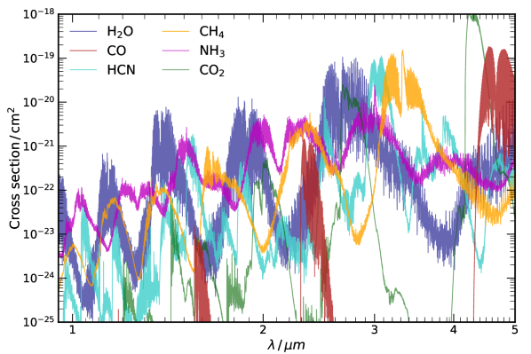
Figure 1: Molecular cross sections for the volatile species discussed in this work. These are shown at a representative temperature of 1000 K and a pressure of 0.1 bar in the 0.95-5 $\mu$m range. The line lists sources for these cross sections are given in Table 1.

Table 1: Line list and pressure broadening references for each of the molecular species.

Species	Line List	Pressure Broadening due to H2/He
H2O	Polyansky et al. (2018)	Petrova et al. (2016); Barton et al. (2017a)
CO	Rothman et al. (2010); Li et al. (2015)	Faure et al. (2013); Gordon et al. (2017)
HCN	Harris et al. (2006); Barber et al. (2014)	Mehrotra et al. (1985); Cohen & Wilson (1973); Charron et al. (1980)
CH4	Hargreaves et al. (2020)	Varanasi & Chudamani (1990); Pine (1992); Gabard et al. (2004)
NH3	Coles et al. (2019)	Barton et al. (2017b)
CO2	Huang et al. (2013); Huang et al. (2017)	Padmanabhan et al. (2014); Gordon et al. (2017)

In what follows, we discuss each line list and the computation of the cross sections in section 2. In section 3 we use the cross sections for each species to generate high resolution spectra for three known exoplanets in transmission or emission and explore the molecular features of each species in their spectra. We then go on in section 4 to explore previous HRS detections of H₂O, CO, HCN and CH₄ in five hot Jupiters and compare and contrast the new cross sections with previous work. Finally we present the discussion and conclusions in section 5.

While the line lists discussed here are currently the most suitable for HRS, they will be continually updated once more complete and accurate line list data becomes available. We make the most up-to-date data publicly available on the Open Science Framework (OSF).

2 Molecular Cross Sections

2.1 Line Lists

The line lists for each molecular species have been chosen to be the most accurate and up to date for temperatures in the range $\sim$500-1500 K typical of the hot Jupiters, warm Neptunes and super Earths we are likely to observe and where they are most prominent. Where available these have been empirically determined to ensure more accurate transition frequencies for high resolution applications.

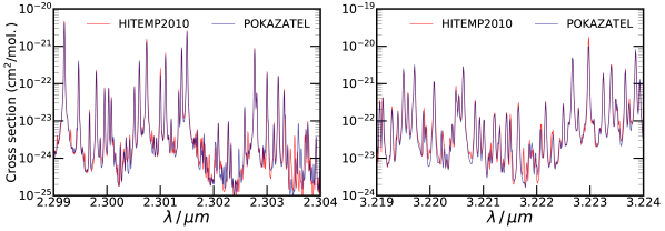
Figure 2: Comparison of the cross sections generated from the H₂O POKAZATEL (Polyansky et al., 2018) and HITEMP (Rothman et al., 2010) line lists. These are generated at 0.01 cm^-1 spacing and shown in the 2.3 $\mu$m (at R$\sim$430,000) and 3.2 $\mu$m band (at R$\sim$310,000), where H₂O has been observed with the CRIRES spectrograph (e.g. Brogi et al., 2013, 2014; Birkby et al., 2013, 2017; Hawker et al., 2018; Cabot et al., 2019). These cross sections are given at a representative temperature of 1000 K and a pressure of 0.1 bar.

2.1.1 H₂O

H₂O is one of the most well studied molecules because of its importance and detectability in exoplanetary atmospheres (e.g. see review by Madhusudhan, 2019). It has been detected with numerous high resolution observations and is one of the dominant sources of opacity for all planets over the temperature range considered here. H₂O is of particular interest for HRS given that observations in some spectral ranges show high signal-to-noise detections whereas other wavelength ranges show absent or weak features for the same exoplanets. For instance, H₂O was detected in the $\sim$3-3.5 $\mu$m range for for $\tau$ Boötis b (Lockwood et al., 2014) but was undetected in the $\sim$2.3 $\mu$m range observations in Brogi et al. (2012), despite H₂O showing strong opacity in both ranges (see Figure 1). To compute our cross sections we use the POKAZATEL line list from ExoMol (Polyansky et al., 2018) which uses ab initio calculations for a fully complete line list up to dissociation. In addition, empirical energy levels (Tennyson et al., 2013) determined with the MARVEL (Measured Active Rotation-Vibration Energy Levels, Furtenbacher et al., 2007) procedure allow for accurate line positions, particularly for the strongest lines which are the most well measured and easiest to detect with HRS. The cross section for H₂O at representative photosphere conditions is shown in Figure 1. It clearly shows strong cross section bands in the $\sim$1.4 $\mu$m, $\sim$1.9 $\mu$m and $\sim$2.7 $\mu$m spectral range.

We compared the POKAZATEL line list to the HITEMP line list (Rothman et al., 2010) at a representative temperature and pressure for the 2.3 $\mu$m and the 3.2 $\mu$m range as shown in Figure 2. The strongest lines show excellent agreement for both line strengths and the transition frequencies. The weaker lines do show some differences, but these are minor and the spectra generated with each remain very similar as they are dominated by the strongest of the lines. Cross correlation with observed spectra also therefore do not show any significant differences between the line lists as discussed further in section 4.1.

As the temperature exceeds $\sim$1200 K, the difference between the two line lists does increase slightly. This is primarily in the spectral regions where the cross section is weaker, such as $\sim$2.2 $\mu$m and $\sim$4 $\mu$m (see Figure 1). This is not unexpected given that experimental verification of the lines at such wavelengths is difficult due to the lower opacity. However, there is a need for accurate line positions for these weaker lines given that high resolution ground based spectroscopy is most accurate in less contaminated regions where telluric absorption from H₂O in the Earth’s atmosphere is weaker.

2.1.2 CO

CO is another species which along with H₂O has been detected in numerous transiting and non-transiting hot Jupiters with HRS. We use the HITEMP CO line list for our work (Rothman et al., 2010; Li et al., 2015). The cross section of CO is shown in Figure 1. This clearly shows distinct bands with a strong cross section at $\sim$1.6 $\mu$m, $\sim$2.3 $\mu$m and $\sim$4.6 $\mu$m. Observations in the 2.3 $\mu$m range were used to detect CO in the transmission spectrum of HD 209458 b (Snellen et al., 2010) and also provide numerous high signal-to-noise detections in emission spectra (e.g. Brogi et al., 2012; Rodler et al., 2012; de Kok et al., 2013; Rodler et al., 2013). The updated HITEMP line list offers more complete coverage at lower wavelengths ($\lesssim$1.6 $\mu$m). This allows us to explore CO at the shorter wavelengths where the ground based HRS observations are able to probe, although it is likely that CO features will be weaker than other species. H₂ and He broadening coefficients for CO are provided in Faure et al. (2013) and Gordon et al. (2017) as shown in table 1. The pressure broadening is unlikely to have a significant impact on HRS detections given that these observations are more sensitive to the line centres at low pressures ($\lesssim$10^-2 bar). However, we include this for completeness and to ensure accuracy for lower resolution observations which are more sensitive to the line wings. At such pressures the broadening can become significant (Hedges & Madhusudhan, 2016).

2.1.3 HCN

We use the ExoMol line list for HCN (Harris et al., 2006; Barber et al., 2014), a high accuracy line list developed for HCN and HNC which has been verified against experimental measurements (Mellau, 2011). We compared the ExoMol line list to HITRAN (Rothman et al., 2013; Gordon et al., 2017) at room temperature and also found excellent agreement. The more complete coverage of this line list means that the cross sections begin to deviate at higher temperatures where other lines increase in strength and thus become more significant. HCN shows significant cross section at $\sim$3.2 $\mu$m (see Figure 1) and two hot Jupiters, HD 209458 b and HD 189733 b, have shown evidence for the species (Hawker et al., 2018; Cabot et al., 2019) in their emission spectra using the ExoMol line list in this spectral range. HCN is expected to be a significant source of opacity for hot Jupiter atmospheres with temperatures $\gtrsim$1500 K when the atmospheric C/O ratio is super-solar (Madhusudhan, 2012; Moses et al., 2013a; Mollière et al., 2015; Drummond et al., 2019).

2.1.4 CH₄

Our CH₄ cross section is calculated from the new HITEMP line list (Hargreaves et al., 2020). This new addition to the HITEMP database utilises ab initio calculations with empirical corrections (Rey et al., 2017) as well as the HITRAN2016 database (Gordon et al., 2017) to produce a high temperature line list up to 2000 K. Hargreaves et al. (2020) found good agreement with experimentally measured opacity at high temperature from Hargreaves et al. (2015) and Wong et al. (2019). The HITEMP line list uses effective lines allowing for efficient computation of opacities for such a large molecule with many billions of transitions. We obtain the H₂ and He pressure broadening coefficients from ExoMol, adopting the a0 coefficients for the present work from the references shown in Table 1. These H₂ and He broadening coefficients are discussed further in section 2.2.3. Recently, high temperature H₂ broadening coefficients have been measured for CH₄ in the 2840-3000 cm^-1 range (Gharib-Nezhad et al., 2019). Such coefficients will be vital to accurately constrain CH₄ as we observe cooler exoplanet atmospheres as chemical models have shown that it is expected to be the dominant carbon bearing species below $\sim$1000 K (Madhusudhan, 2012; Moses et al., 2013a; Drummond et al., 2019). We will therefore constantly update the cross sections to provide the most accurate for both low- and high-resolution spectroscopy of exoplanet atmospheres.

2.1.5 NH₃

The NH₃ line list comes from ExoMol (Coles et al., 2019) and covers the whole infrared range considered in this work (0.95-5 $\mu$m). This line list has also been corrected using empirical energy levels (Al Derzi et al., 2015; Coles et al., 2020) up to 6000 cm^-1 ($\gtrsim$1.66 $\mu$m) generated using the MARVEL procedure and is hence ideal for HRS. Numerous strong features can be seen in the cross section in Figure 1 at $\sim$1.6 $\mu$m (H band) and $\sim$2.2 $\mu$m (K band). It may potentially be detectable with low resolution observations of hot Jupiters if present at sufficient abundance (MacDonald & Madhusudhan, 2017). The higher sensitivity of HRS to trace species mean that the high accuracy ExoMol line list may be key to robust constraints of NH₃ in the future. In addition, the latest generation of high resolution spectrographs may also be able to explore cooler planets with temperatures $\lesssim$1000 K where NH₃ may be more abundant with $\log(X_{\mathrm{NH_{3}}})\gtrsim-5$ (Moses et al., 2013b).

2.1.6 CO₂

The Ames line list for CO₂ (Huang et al., 2013; Huang et al., 2017) offers accurate line positions and transition strengths with a root mean square deviation of $\lesssim$0.02 cm^-1 in line position from experimentally determined values. This accuracy is required for HRS given the high resolution observations. Tentative constraints of CO₂ have been observed in previous low resolution and high resolution observations (Stevenson et al., 2010; Birkby et al., 2013), but further observations are needed to confirm the presence of the species. CO₂ is expected to become prominent at cooler temperatures $\lesssim$1000 K. This is particularly so as we explore non H₂-rich atmospheres, where it is expected to be highly abundant in the atmosphere for metallicities $\gtrsim$1000$\times$ solar (e.g. Moses et al., 2013b).

2.2 Determining the Cross Section

Table 2: The temperature and pressure grid for our cross sections. The cross sections are generated at each pressure and temperature at 0.01 cm^-1 wavenumber spacing in the 0.95-5 $\mu$m range (10,526-2000 cm^-1).

T(K)	400	600	800	1000	1200	1400	1600
P(bar)	$10^{-5}$	$10^{-4}$	$10^{-3}$	$10^{-2}$	$10^{-1}$	1	10

We now discuss how we calculate the cross section from the line list of each molecular species. Table 2 shows the grid that we compute the cross sections on, ranging between 400-1600 K in temperature and 10^-5-10 bar in pressure. At each pressure and temperature the lines are spectrally broadened into a Voigt profile according to the method in Gandhi & Madhusudhan (2017). We compute the cross sections in the infrared on a uniform grid of 0.01 cm^-1 wavenumber spacing between 10,526-2000 cm^-1 (0.95-5 $\mu$m). This corresponds to a spectral resolution of $\mathrm{R}=10^{6}$ at 1 $\mu$m. To compute the pressure broadening we use the latest H₂ and He broadening coefficients obtained from sources listed in Table 1. In addition, we also include the natural broadening of each line which arises from the uncertainty principle (Gray, 1976). The summed contribution from each line in the line list gives the overall cross section for each species. We first describe how to compute the line strengths at each temperature, followed by the broadening procedure.

2.2.1 Line Strengths

As the temperature is changed the populations within each of the states are altered and hence the line strengths of each line in a line list, $S(T)$, also vary. These line strengths are often provided in the line lists relative to a reference temperature (e.g. 296 K). The line strength at a general temperature $T$ is then calculated from these by (Gordon et al., 2017),

$$S(T) =S_{0}\frac{Q(T_{\mathrm{ref}})}{Q(T)}\frac{\mathrm{exp}(-E_{\mathrm{lower}}/k_{b}T)}{\mathrm{exp}(-E_{\mathrm{lower}}/k_{b}T_{\mathrm{ref}})}\frac{1-\mathrm{exp}(-\nu_{0}/k_{b}T)}{1-\mathrm{exp}(-\nu_{0}/k_{b}T_{\mathrm{ref}})},$$ (1)

where $S_{0}$ is the line strength at the reference temperature $T_{\mathrm{ref}}$. $E_{\mathrm{lower}}$ is the lower energy state of the transition (in cm^-1) and $\nu_{0}$ is the frequency of the transition ($E_{\mathrm{upper}}-E_{\mathrm{lower}}=\nu_{0}$). The partition function $Q$ is

$$Q(T) =\sum_{j}g_{j}\mathrm{exp}(-E_{j}/k_{b}T)$$ (2)

with the degeneracy of the state $j$ given by $g_{j}$ and where $k_{b}$ is the Boltzmann constant (in cm^-1 K^-1). The line strength $S(T)$ can also be calculated directly through the Einstein coefficient $A$ of a transition,

$$S(T) =\frac{Ag}{8\pi c\nu_{0}^{2}}\frac{\mathrm{exp}(-E_{\mathrm{lower}}/k_{b}T)}{Q(T)}(1-\mathrm{exp}(-\nu_{0}/k_{b}T)).$$ (3)

We must calculate the line strength of each line at each temperature that the cross sections are computed.

2.2.2 Thermal and Pressure Broadening

Every line is broadened according to the temperature and pressure in order to determine the cross section as a function of frequency. The broadening due to the temperature is caused by the velocity distribution of the molecules in the gas which Doppler shifts the transition frequency according to the distribution of speeds. This results in each transition line being spread over frequency. In this case the thermal broadening results in a Gaussian line profile (Hill et al., 2013), given by

$$f_{G}(\nu-\nu_{0}) =\frac{1}{\gamma_{G}\sqrt[]{\pi}}\mathrm{exp}\left(-\frac{(\nu-\nu_{0})^{2}}{\gamma_{G}^{2}}\right),$$ (4)

$$\gamma_{G} =\sqrt[]{\frac{2k_{b}T}{m}}\frac{\nu_{0}}{c},$$ (5)

where $\nu$ and $\nu_{0}$ represent the frequency and the line transition frequency respectively (in cm^-1). Here, $m$ represents the mass (in kg) of the molecule and $T$ represents the temperature (in K).

Collisions with other molecules at pressure alters each molecule’s state decay times and results in a Lorentzian profile with frequency. In addition to this, each line is also naturally broadened due the uncertainty principle (Gray, 1976). This is often much weaker than pressure broadening, particularly in the photospheres of exoplanets in our HRS observations, but we include this effect for completeness. The combined Lorentzian profile from pressure and natural broadening is given by

$$f_{L}(\nu-\nu_{0}) =\frac{1}{\pi}\frac{\gamma_{L}}{(\nu-\nu_{0})^{2}+\gamma_{L}^{2}},$$ (6)

$$\gamma_{L} =P\sum_{i}\left(\frac{T_{\mathrm{ref}}}{T}\right)^{n_{i}}\gamma_{i}\,X_{i}+\gamma_{N},$$ (7)

$$\gamma_{N} =0.22\times 10^{-2}\frac{\nu_{0}^{2}}{4\pi c}$$ (8)

where $\gamma_{L}$ and $\gamma_{N}$ are Lorentzian and natural values of the corresponding half-widths-at-half-maximum (HWHM) and $X_{i}$ is the mixing ratio of a specific broadening species $i$. The pressure broadening coefficients $\gamma_{i}$ and $n_{i}$ represent the Lorentzian HWHM and the power law for the temperature respectively. A reference temperature $T_{\mathrm{ref}}$ of 296 K is most commonly used. In our work the pressure broadening is included from from $i=\mathrm{H_{2}}$ and $i=\mathrm{He}$ (Table 1), with the mixing ratio $X_{i}$ set from solar abundances (Asplund et al., 2009).

Natural broadening arises as a result of the finite lifetime of a state which results in a $\Delta\nu$ from the uncertainty principle. The 0.22$\times 10^{-2}$ factor in the natural broadening width has been derived for hydrogen (Gray, 1976) but we use this value for all of the species in our work given the absence of any other calculated values. The value of $\gamma_{N}$ for Sodium with experimental measurements of one of the the Na D line transitions at $\sim$0.589 $\mu$m (Bernath, 2015) does show good agreement. The natural broadening is relatively weak compared to thermal and pressure broadening unless considering low pressures and temperatures and high wavenumbers so any differences that may arise for species in our work are also less of a concern.

The full broadening profile is a convolution of the Gaussian from thermal broadening and the Lorentzian profile. This is known as a Voigt function,

$$f_{V}(\nu-\nu_{0}) =\int_{-\infty}^{\infty}f_{G}(\nu^{\prime}-\nu_{0})f_{L}(\nu-\nu^{\prime})d\nu^{\prime}.$$ (9)

Defining

$$u \equiv\frac{\nu-\nu_{0}}{\gamma_{G}},$$ (10)

$$a \equiv\frac{\gamma_{L}}{\gamma_{G}},$$ (11)

the Voigt function can be cast in terms of the real part of the normalised Faddeeva function, $w(x+iy)$, to

$$f_{V}(\nu-\nu_{0},\gamma_{L},\gamma_{G}) =\frac{\mathrm{Re}(w(u+ia))}{\gamma_{G}\sqrt[]{\pi}}.$$ (12)

The cross section $\sigma_{\nu}$ at a frequency $\nu$ for a transition line with strength $S(T)$ is then given by (Gandhi & Madhusudhan, 2017)

$$\sigma_{\nu}=S(T)f_{V}(\nu-\nu_{0},\gamma_{L},\gamma_{G}).$$ (13)

The temperature and pressure grid used to compute the cross sections is given in Table 2 and encompasses typical ranges likely in the photosphere. We have ignored the frequency shifts of the line positions with pressure for all species except CO as these are negligible for our work.

2.2.3 Pressure Broadening Coefficients

Table 1 shows the references for the broadening coefficients $n_{i}$ and $\gamma_{i}$ for each of the volatile species. For each species we use H₂ and He broadening to work out the cross section as a function of wavelength for each pressure and temperature. We calculate the broadened lines out to 500 Voigt widths according to previous works Hedges & Madhusudhan (2016); Gandhi & Madhusudhan (2017). This corresponds to a minimum line extent of $\sim$20 cm^-1. The broadening coefficient files are provided on the ExoMol database. The coefficients are determined by the J-quantum numbers of each transition. We adopt the a0 coefficients for our present work which requires only the lower state J-quantum number. We then determine the overall $n_{i}$ and $\gamma_{i}$ by summing over the H₂ and He broadening coefficients weighted by their abundance. However for CO₂ these coefficients were not available so we adopt $\gamma_{i}=0.11$ cm^-1/atm from Padmanabhan et al. (2014) and $n_{i}$ from HITRAN (Gordon et al., 2017).

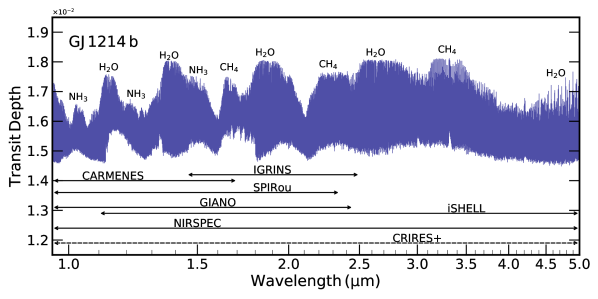
Figure 3: The cloud free transmission spectrum of GJ 1214 b showing the transit depth with wavelength. We also show the spectral ranges for the current generation of high resolution spectrographs. The upcoming CRIRES+ on the VLT has been marked with a dashed line as the exact formatting of the orders has not yet been determined, hence we show the full observable range.

3 Model Spectra

We will now use the cross sections generated from the line lists as discussed in section 2 to accurately model the spectra of known super Earths, warm Neptunes and hot Jupiters. We model three exoplanets with a range in mass, radius and equilibrium temperature to explore the spectral features of each species in the infrared spectrum. Most current observations target hot Jupiters, and therefore do not encompass the full range of systems observable today. Surveys such as TESS (Ricker et al., 2015) will find more warm Neptunes and super Earths suitable for characterisation with HRS and hence we also model the spectra of these cooler targets. We generate spectra using GENESIS (Gandhi & Madhusudhan, 2017) for emission and AURA (Pinhas et al., 2018) for transmission. The spectra have been generated to match the cross section grid at a wavenumber spacing of 0.01 cm^-1 in the 0.95-5 $\mu$m range. In addition to the opacity from the molecular species, we also include collisionally induced absorption (CIA) from H₂-H₂ and H₂-He interactions (Richard et al., 2012).

We begin with the super Earth/sub-Neptune GJ 1214 b, and then discuss the warm sub-Neptune GJ 3470 b. In spite of the observational evidence for clouds in these two exoplanets, in this work we model the cloud free spectrum as a representative case for each exoplanet class. Both of these are modelled under transmission geometries given that the lower temperatures and smaller radius make thermal emission more difficult to detect. Hence transmission spectroscopy of super Earths and warm Neptunes will likely produce the strongest detections and constraints on the volatile molecular species. In addition, we also model the dayside emission spectrum of HD 189733 b, a hot Jupiter, which has had H₂O, CO and HCN detected in the dayside atmosphere (Birkby et al., 2013; Rodler et al., 2013; Cabot et al., 2019).

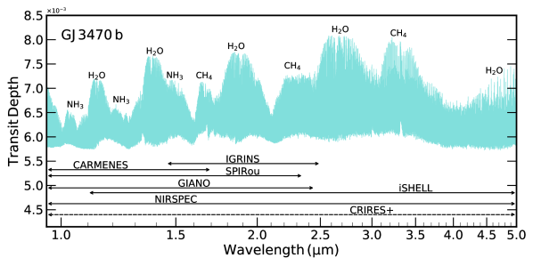
Figure 4: The cloud free transmission spectrum of GJ 3470 b showing the transit depth with wavelength. We also show the spectral ranges for the current generation of high resolution spectrographs. The upcoming CRIRES+ on the VLT has been marked with a dashed line as the exact formatting of the orders has not yet been determined, hence we show the full observable range.

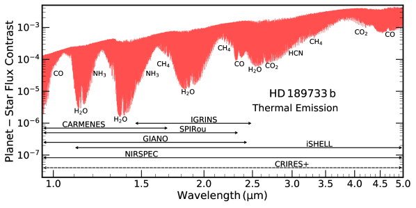
Figure 5: Planet-star flux ratio in the thermal emission spectrum of HD 189733 b. We model a radiative-convective equilibrium atmosphere (Gandhi & Madhusudhan, 2017) with the volatile molecular species in chemical equilibrium at solar abundance. We also show the spectral ranges for the current generation of high resolution spectrographs. The upcoming CRIRES+ on the VLT has been marked with a dashed line as the exact formatting of the orders has not yet been determined, hence we show the full observable range.

3.1 Super Earth/Sub-Neptune: GJ 1214 b

The exoplanet GJ 1214 b has a radius of $\sim$2.6 R_⊕ and a mass of $\sim$6.5 M_⊕ and is one of the coolest exoplanets observed thus far with an equilibrium temperature of $\sim$550 K (Carter et al., 2011). We model the cloud free spectrum at 100$\times$ solar abundance, with $\log(\mathrm{H_{2}O})=-1.2$, $\log(\mathrm{CH_{4}})=-1.5$ and $\log(\mathrm{NH_{3}})=-2$. This is shown in Figure 3. This shows a highly varied transit depth with wavelength due to opacity from the molecular species present in the atmosphere. The broad molecular absorption bands from the cross section of each of the species result in the planet’s atmosphere becoming opaque at higher altitudes. This results in a larger effective planet radius and hence transit depth. Molecular features which result form the cross section of each species can clearly be seen in the spectrum. The molecule corresponding to each spectral feature is highlighted in the spectrum in Figure 3.

Numerous strong spectral lines can be seen for H₂O, CH₄ and NH₃ for cross correlation in the infrared. The spectrum is dominated by the absorption of H₂O due to its large cross section and abundance. CH₄ also shows some strong features, particularly in the $\sim$1.8 $\mu$m and $\sim$3.5 $\mu$m range where it has a strong cross section. The NH₃ on the other hand has generally weaker spectral signatures than the H₂O and CH₄ due to the lower abundance. However, features can clearly be seen in the spectral ranges where H₂O and CH₄ opacity is weak. We have modelled the cloud free atmosphere to demonstrate the new high resolution cross sections in this work but we note that GJ 1214 b has shown evidence for a high altitude cloud deck (Bean et al., 2010; Berta et al., 2012; Kreidberg et al., 2014a). Cloudy atmospheres reduce the extent of spectral features, making detections more difficult due to the shallower spectral lines for each species. Understanding how cloudy exoplanets affect high resolution spectroscopy is thus extremely important for robust detections and will be extensively treated in the future but is beyond the scope of our current work.

3.2 Warm Neptune: GJ 3470 b

The exoplanet GJ 3470 b is more massive than GJ 1214 b with a mass of $\sim$12 M_⊕ and thus falls into the category of warm sub-Neptunes. This planet also has a higher equilibrium temperature of $\sim$650 K. The atmosphere of GJ 3470 b has recently been observed with HST WFC3, HST STIS and Spitzer spectrographs and shown evidence for H₂O in the atmosphere at solar abundance (Benneke et al., 2019). The cloud free transmission spectrum is shown in Figure 4. Despite the larger planet radius, the transit depth is lower than for GJ 1214 b due to the larger stellar radius. Here, we have assumed a temperature profile based on the best fit retrieval in Benneke et al. (2019), which indicated that the upper layers of the atmosphere were at $\sim$600 K, consistent with the equilibrium temperature. We have modelled this atmosphere assuming a solar abundance of the volatile species, with $\log(\mathrm{H_{2}O})=-3.2$, $\log(\mathrm{CH_{4}})=-3.5$ and $\log(\mathrm{NH_{3}})=-4$. Numerous spectral features can be seen for the volatile species throughout the infrared. As with GJ 1214 b, the atmosphere is dominated by the strong absorption from H₂O and CH₄, with weaker features from NH₃. The spectral features are generally weaker than for GJ 1214 b due to the lower atmospheric abundance of each species.

3.3 Hot Jupiter: HD 189733 b

The hot Jupiter HD 189733 b is one of the most well observed exoplanets in both low resolution (Tinetti et al., 2007; Crouzet et al., 2014) and high resolution under emission given its strong signature from its extended hot H₂-rich atmosphere. Previous high resolution observations of the dayside with CRIRES, NIRSPEC and CARMENES have shown evidence for H₂O (Birkby et al., 2013; Alonso-Floriano et al., 2019), CO (Rodler et al., 2013; de Kok et al., 2013) and HCN (Cabot et al., 2019). We model the dayside atmosphere of this hot Jupiter in chemical and radiative-convective equilibrium assuming a non-inverted pressure-temperature profile (Gandhi & Madhusudhan, 2017), consistent with the observational constraints.

Figure 5 shows the planet-star flux ratio for HD 189733 b. This shows that at such high temperatures ($\sim$1400 K) the spectrum is dominated by the presence of H₂O and CO. CH₄ and NH₃ are now at lower abundances in the atmosphere due to the higher temperature. Hence only small absorption features can be seen from CH₄, NH₃, CO₂ and HCN and only in the spectral ranges where the H₂O and CO absorption is weak. However, the current generation of spectrographs are still be able to detect some of these trace species (Cabot et al., 2019) in the atmosphere due to the strong emission from the planet, particularly if the atmospheric C/O ratio is super-solar to potentially enhance their abundance (Madhusudhan, 2012; Moses et al., 2013a; Drummond et al., 2019).

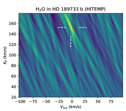
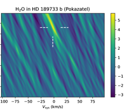
Figure 6: H₂O signal obtained by cross correlating VLT/CRIRES spectra of exoplanet HD 189733 b around 3.2 $\mu$m with a best-fitting model matching the parameters of Birkby et al. (2013) and using either opacities from Rothman et al. (2010) (left panel) or the newest opacities from Polyansky et al. (2018) (right panel). The cross correlation signal is shown as function of systemic velocity $V_{\mathrm{sys}}$ and maximum orbital radial velocity $K_{\mathrm{P}}$ and shows excellent agreement between the two models, both in terms of localisation and strength. The known values of (-2.4, 151) km s^-1 are marked with dashed white lines and are a good match to these observations.

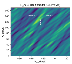
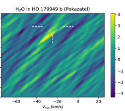
Figure 7: H₂O signal obtained by cross correlating VLT/CRIRES spectra of exoplanet HD 179949 b around 2.3 $\mu$m with a best-fitting model matching the parameters of Brogi et al. (2014) and using either opacities from Rothman et al. (2010) (left panel) or the newest opacities from Polyansky et al. (2018) (right panel). The cross correlation signal is shown as function of systemic velocity $V_{\mathrm{sys}}$ and maximum orbital radial velocity $K_{\mathrm{P}}$. Although the two models show a signal in qualitative agreement, the best-fitting planet radial velocity semi-amplitude is in tension with the value obtained from the combined CO+H₂O analysis (dashed white lines).

4 Validation on Existing Observations of Hot Jupiters

We now explore previous detections of molecular species with HRS in the atmospheres of hot Jupiters using the cross sections developed in section 2. These hot Jupiter atmospheres have been extensively observed in a number of spectral ranges in the infrared at R$\gtrsim$50,000 from observational facilities such as CRIRES/VLT and GIANO/TNG. We discuss five hot Jupiters, HD 189733 b, HD 179949 b, $\tau$ Boötis b, HD 209458 b and HD 102195 b, which have shown evidence for H₂O, CO, HCN and CH₄. We use the cross sections computed in section 2 to calculate the high resolution spectrum using GENESIS (Gandhi & Madhusudhan, 2017). For each case we use the best fit parameters from each detection (Birkby et al., 2013; Brogi et al., 2014, 2012; Hawker et al., 2018; Guilluy et al., 2019). We then use these spectra to cross correlate against observations following the same procedure as discussed in previous work.

Unless explicitly specified, observations are processed as in the published detection papers, i.e. they use the same calibration and removal of telluric and stellar lines. The only difference is that we use the models described in this work to compute the cross correlation.

In what follows we adopt a threshold of S/N=3 to claim a tentative detection, and a S/N$>$4 to claim a definite detection.

4.1 H₂O: HD 189733 b

H₂O was first detected using low-resolution Spitzer data (Tinetti et al., 2007) and confirmed with HRS in the dayside spectrum of HD 189733 b observed between 3.18 and 3.27 $\mu$m using the CRIRES spectrograph (Birkby et al., 2013). Subsequent transmission spectra with GIANO (Brogi et al., 2018) and CARMENES (Alonso-Floriano et al., 2019) have also shown evidence for H₂O in the atmosphere of this planet. We utilise the CRIRES observations from Birkby et al. (2013), calibrated as in their work for the alignment to the common reference frame of the Earth’s atmosphere and the determination of the pixel-wavelength solution. Following the prescriptions of their work, we limit the analysis to detector 1 and 3 of CRIRES, given that detector 2 is affected by very low telluric transmission and detector 4 by a well-documented instrumental issue. We additionally also use the same mask as Birkby et al. (2013) for our work. We use a more straightforward detrending algorithm than Sysrem to remove telluric and stellar lines based on singular-value decomposition (SVD), which does not allow for unequal error bars on the data points. We remove the same number of eigenvectors (9 for detector 1 and 3 for detector 3), and verify that as in the case of Birkby et al. (2013) this is the optimal number of components to maximise the signal. The use of SVD over Sysrem increases the signal-to-noise ratio of the measured signals by about 0.7, regardless of the line list used to produce the model spectrum used for cross correlation.

As we show in Figure 6, we recover a detection of water vapour at a S/N = 5.7 and at the expected planet position. We note that we obtain a comparable signal and very similar noise structure when we cross correlate with the best-fitting model of Birkby et al. (2013), which also contains water but from HITEMP (Rothman et al., 2010). We therefore quantitatively confirm the result shown in Figure 2 (right panel), and report a strong agreement between two different line lists for water around 3.2$\mu$m.

4.2 H₂O: HD 179949 b

Detection of water vapour in $K$-band CRIRES observations (2.27-2.35 $\mu$m) has been somewhat less convincing compared to the cases reported in Section 4.1. This is not completely unexpected, given that this spectral window is far from the main opacity peaks of water vapour (see Figure 1), and CO is the main opacity source. Consequently, water alone has produced either no signals (Brogi et al., 2012, 2017; Brogi & Line, 2019), or signals that are just above the threshold of detectability (Brogi et al., 2014; Gandhi et al., 2019), but still strengthening the cross correlation substantially when modelled in conjunction with CO. In this paper we re-examine one of the latter cases, namely 3 half-nights of dayside spectroscopy of the non-transiting planet HD 179949 b (Brogi et al., 2014). Here water was detected at a S/N = 3.9, and with a noise pattern in velocity space marginally inconsistent with the detection coming from CO (S/N = 5.8). When combined, however, the cross correlation from the two species was shown to co-add constructively and deliver a convincing S/N = 6.3, or a significance of 5.8$\sigma$.

We have modelled the atmosphere of HD 179949 b with a pressure-temperature ($P-T$) profile consistent with the family of best-fitting models in (Brogi et al., 2014), and a water abundance of 10^-4.5. Once again, we have utilised cross sections computed from both HITEMP (Rothman et al., 2010) and POKAZATEL (Polyansky et al., 2018). The resulting cross correlation is shown in Figure 7. In spite of a qualitative agreement between the two signals and the overall noise structure, there is a net departure from the best-fitting velocities obtained from the combined H₂O+CO model. The cross correlation seems to be double-peaked, where the primary peak at lower $K_{\mathrm{P}}$ is just above the threshold for marginal detection (S/N = 3.2) with HITEMP, but peaks at S/N = 4.1 with POKAZATEL. Furthermore, the secondary peak matching the $K_{\mathrm{P}}$ of (Brogi et al., 2014) is marginally detected in both cases, albeit slightly more convincingly with the HITEMP line list.

There are arguably astrophysical reasons that could produce a mismatch between velocities measured with two different species, e.g., strong atmospheric patterns variable with pressure. However, if we did not have any prior knowledge of the planet’s orbit and only rely on water alone, we could be deriving a biased value of its radial velocity semi-amplitude, which consequently would affect both the inferred planet mass and orbital inclination. As the detection of water in HD 179949 b is just above marginal, we cannot firmly conclude that there is a potential influence of water line lists on results derived with $K$-band spectra. We point out instead that further investigation and possibly a larger amount of data is required to identify the possible reasons of this discrepancy.

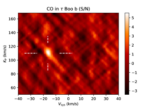
Figure 8: CO signal obtained by cross correlating VLT/CRIRES spectra of exoplanet $\tau$ Boötis b around 2.3 $\mu$m with a CO model matching the best-fit parameters of Brogi et al. (2012). The cross correlation signal is shown as function of systemic velocity $V_{\mathrm{sys}}$ and maximum orbital radial velocity $K_{\mathrm{P}}$. The known values of (-16.4, 110) km s^-1 are marked with dashed white lines and are a good match to these observations.

4.3 CO: $\tau$ Boötis b

This dataset consists of three half nights of observations (approximately 3 $\times$ 6 hours including overheads) of the non-transiting planet $\tau$ Boötis b. The spectra are observed with CRIRES at the Very Large Telescope and span the spectral range 2.29-2.35 $\mu$m, where CO possesses strong absorption (see Figure  1). As in Brogi et al. (2012), we exclude detectors 1 and 4 from the analysis and weigh the cross correlations from each spectrum and each detector equally. Results from the cross correlation analysis are presented in Figure 8. We confirm the detection of Brogi et al. (2012) at a compatible S/N of 5.6 and at the same values of planet systemic velocity ($V_{\mathrm{sys}}=-16.4$ km s^-1) and maximum orbital radial velocity ($K_{\mathrm{P}}=110$ km s^-1). Consistently with Brogi et al. (2012), we find a marginal increase of the cross-correlation signal when including water as additional species. However, water-only models do not result in a detection above the threshold of S/N=3. Indeed, based on the increase in S/N with the mixed H₂O + CO model, we estimate that water vapour can only contribute by S/N$\leq 2$.

4.4 HCN: HD 209458 b

Evidence for HCN was first presented by Hawker et al. (2018) based on the analysis of high resolution dayside observations of the hot Jupiter HD 209458 b obtained with CRIRES. We use their processed spectra for what concerns pixel-wavelength calibration, and removal of telluric lines through the Sysrem algorithm. We generate a model spectrum with the best fit parameters in Hawker et al. (2018), corresponding to an atmospheric abundance of 10^-5, and including $\gtrsim 4\times 10^{5}$ transitions in the observed spectral range (3.18-3.27 $\mu$m).

As shown in figure 9, we recover the detection of HCN at a S/N of 4.8 at the expected planetary radial velocity semi-amplitude and systemic velocity. The S/N of the recovered signal is fully consistent with previous work (Hawker et al., 2018) and the two dimensional velocity map (K_p and V_sys in the 3.18-3.27 $\mu$m range) also shows a very similar noise structure. This is in line with expectations, given that we use the same ExoMol line list, which is updated to include H₂ and He broadening. Our model thus has nearly identical line positions and strengths as the best fitting model of Hawker et al. (2018).

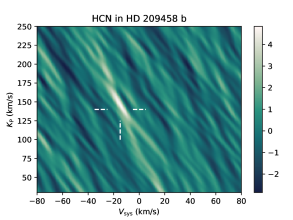
Figure 9: HCN signal obtained from cross correlation of L-band VLT/CRIRES spectra of exoplanet HD 209458 b with a best-fitting model matching the parameters of Hawker et al. (2018). We confirm a detection at a S/N = 4.8 and at the expected planet systemic and orbital radial velocity, indicated by the white dashed lines.

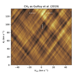
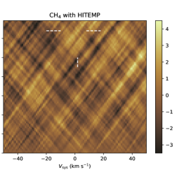
Figure 10: Cross correlation of models with methane as molecular species and dayside spectra of exoplanet HD 102195 b processed as in Guilluy et al. (2019). Left panel: cross correlation with models containing cross sections computed from HITRAN2016 (Gordon et al., 2017). Right panel: cross correlation with a model containing the recent HITEMP line list (Hargreaves et al., 2020). Cross correlation are given as function of systemic velocity and maximum orbital radial velocity.

4.5 CH₄: HD 102195 b

The first detection of methane at high spectral resolution was only recently reported by Guilluy et al. (2019), who analysed three half-nights of dayside spectra of the non transiting planet HD 102195 b observed with GIANO at the Telescopio Nazionale Galileo. The spectra span orbital phases prior, around, and post superior conjunction, and this sampling was adopted to obtain the tightest constraint on the orbital parameters of the exoplanet, as done in the case of $\tau$ Boötis b. In this work for full consistency we utilise the data processed and masked as in Guilluy et al. (2019), resulting in coverage of most the $K$ band (2.1-2.4 $\micron$ split in 4 or 5 spectral orders), part of the $H$-band (2-3 orders in the range 1.6-1.8 $\micron$) and part of the J band (2 orders between 1.0-1.2 $\micron$) at a resolving power of 50,000. We simultaneously use all of the available orders across all three bands for our analysis. This choice corresponds to 9 or 10 orders (variable with the observing night) out of 50, and matched the choices in Guilluy et al. (2019). The incomplete coverage results from combination of a challenging wavelength calibration of some of the spectral orders, and the choice to only include the orders corresponding to the highest methane cross section, as shown for instance in Figure 1.

In Figure 10 we present the total cross correlation signal coming from two different models. The former, shown on the left panel, is obtained with cross section computed from the full list of lines published by the HITRAN group (Gordon et al., 2017) at the time of the publication of Guilluy et al. (2019). The total cross correlation signal is comparable to their work in terms of both strength (S/N = 4.6) and position in velocity space. The latter model, shown on the right panel, utilises the cross sections described in this paper and obtained from the HITEMP database (Hargreaves et al., 2020). This model shows no significant correlation at the expected position of the planet (marked by dashed lines), thus we are unable to confirm the detection with this more recent line list.

In interpreting this result, the following elements need to be considered. Firstly, we note that the detection of Guilluy et al. (2019) is substantiated by the simultaneous measurement of water vapour at compatible velocities. This allows the signal of the two molecular species to coherently combine when a model containing CH₄+H₂O is used for cross correlation. We are indeed able to reproduce the detection of water vapour in this study. Secondly, by looking at the right panel of Figure 10, we also note that from data spanning a large range in orbital phase we would expect a much tighter localisation of the cross correlation peak, e.g. the spot-like detection observed from CO in $\tau$ Boötis b (see section 4.3). The qualitative difference in the shape of the cross-correlation peak could be due to the fact that this non-transiting exoplanet has a poorly constrained orbital solution. By propagating the error bars in orbital period and time of inferior conjunction, we estimate an uncertainty of about 10% in orbital phase.

Thirdly, we highlight significant differences between the spectra produced with HITRAN2016 and HITEMP. While all the strong spectral lines agree well between the two spectra, the overall continuum level does not, and this is expected because HITEMP is much more complete at high temperatures, therefore raising the overall opacity due to methane. This increased opacity mutes some of the lines that in the HITRAN spectrum would appear as strong lines, and add a dense forest of weaker lines that were not present at all, therefore potentially affecting the cross correlation signal if these weaker lines carry a non-negligible weight. In order to assess their importance we show the auto-correlation of each of the models in Figure 11, compared to their mutual cross-correlation signal. The latter peaks at a correlation value of 0.56, which indicates that a non-negligible fraction of the signal is carried by the weak lines present in HITEMP, but absent in HITRAN2016. As a consequence, if neglected when interpreting observations, the resulting cross correlation signal could be significantly muted. On the other hand, if these lines are included in the models but suffer from inaccuracies at the resolving power of the observations, this could also hamper the methane signal preventing detection.

The assumed P-T profile of the atmosphere may also more strongly impact the HITEMP model spectrum. The weaker spectral lines are more numerous and generally vary more significantly with temperature compared to the strongest lines. Thus if the overall atmospheric temperature is less than that assumed in the model, the more complete HITEMP line list may perform worse as the many more weak lines contribute to reduce the overall correlation with the data. We tested this by cross correlating the data with models of HD 102195 b generated with a P-T profile that was 300 K cooler. This was the coolest P-T profile that remained consistent with the expected physical conditions from the orbit of the planet. With this cooler temperature profile the cross correlation between the HITEMP and HITRAN2016 models did improve to $\sim$0.62 but we found no significant improvement in the overall signal with the HITEMP line list. This shows that while the contribution from the weak lines present in HITEMP reduces as we approach cooler temperatures, this change is not significant enough to explain the current differences in our findings.

We also note that the CH₄ cross section is most accurately determined at low wavenumbers (Hargreaves et al., 2020) and this may also influence the overall detection if it is dominated by the higher frequency bands such as the H band. Based on the limited data presented here and the inaccuracy of the orbital solution, in this context we limit to report these caveats and we conclude that it is still challenging to derive firm prescriptions on the methane cross sections without a dedicated follow-up study.

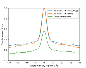
Figure 11: Auto-correlation function of the model computed with HITRAN2016 (blue line), HITEMP (orange line), and the cross correlation function of the two models (green line). The latter peaks at 0.56, highlighting substantial differences in the spectral features contained by the two models.

5 Discussion and Conclusions

We present new publicly available high resolution cross sections for the volatile molecular species expected to be prominent in hot Jupiters, warm Neptunes and super Earths with temperatures ranging from $\sim$500-1500 K. We focus on species with observable signatures from current ground based facilities in the near infrared. This leads us to consider line lists sources for six species, namely H₂O, CO, HCN, CH₄, NH₃ and CO₂, which are given in Table 1. We compute the cross sections for these species in the wavelength range 0.95-5 $\mu$m (2000-10,526 cm^-1) at a wavenumber spacing of 0.01 cm^-1. This corresponds to a spectral resolution of $\mathrm{R}=10^{6}$ at 1 $\mu$m. We summarise the key developments of the cross sections below.

• The line list sources for the cross sections are given in Table 1 and use the ExoMol (Tennyson et al., 2016), HITEMP (Rothman et al., 2010; Hargreaves et al., 2020) and Ames (Huang et al., 2017) databases.

• These line lists were chosen as they typically use ab initio calculations combined with experimentally verified line positions for maximum accuracy in the line position. This is key for detections with HRS in order to maximise the cross correlation with the observations.

• The completeness of the line lists in the spectral range provided also ensures that the high resolution cross sections computed in this work are optimised for use in low resolution spectra.

• Each line is broadened according to the pressure and temperature from the grid given in Table 2. This grid of $P-T$ values was chosen to represent typical photosphere conditions of super Earths, warm Neptunes and hot Jupiters. The overall line profile of each transition in a line list is a Voigt function resulting from a convolution of a Gaussian from thermal broadening and a Lorentzian from pressure broadening. In addition, natural broadening has been included which occurs from the uncertainty principle which also results in a Lorentzian line shape (Gray, 1976).

• We use the latest H₂ and He pressure broadening for the cross sections of each species thanks to recent work on pressure broadening coefficients (see Table 1). This allows for more accurate cross sections of these planets at high pressure. These pressure broadening coefficients are particularly beneficial for accurate low resolution spectra which are more sensitive to the line wings where this is the dominant source of broadening (Hedges & Madhusudhan, 2016).

• As more accurate and complete line lists become available in the near future we will continually update our cross sections to ensure that the most up to date are available.

We use the cross sections calculated in this work to generate spectra of known planets to identify spectral features of each species in the infrared. We model the atmosphere of three exoplanets, the super Earth/sub-Neptune GJ 1214 b, the warm sub-Neptune GJ 3470 b and the hot Jupiter HD 189733 b, chosen to have a wide range in mass, radii and equilibrium temperatures. We find that H₂O has prominent spectral features throughout the infrared for each of the exoplanets modelled given its abundance and strong cross section. CO on the other hand only has strong features for hot Jupiters such as HD 189733 b where it is expected to be more abundant (e.g. Madhusudhan, 2012). The abundance and hence spectral features of other species such as HCN can be strongly affected by the atmospheric C/O ratio in hot Jupiters (Moses et al., 2013a; Drummond et al., 2019). The cooler planets GJ 1214 b and GJ 436 b show prominent spectral features for CH₄ and NH₃ given the higher abundance for these two planets. In particular, the strongest features for these species occur in the wavelength ranges where H₂O absorption is weak. This thus represents an exciting opportunity in the future for chemical detections using HRS which typically probe in between H₂O bands where many of these features may be detectable.

We also use our new cross sections to generate high resolution spectra of hot Jupiters which have shown evidence for these volatile molecular species from previous observations (Birkby et al., 2013; Brogi et al., 2014, 2012; Hawker et al., 2018; Guilluy et al., 2019) to validate our opacities. We model the best fitting spectra of HD 189733 b and HD 179949 b with H₂O, $\tau$ Boötis b with CO, HD 209458 b with HCN and HD 102195 b with CH₄ using GENESIS (Gandhi & Madhusudhan, 2017). We then perform cross correlation on the observations following similar data analysis techniques discussed in previous works. We reproduce the high signal to noise detections seen for H₂O, CO and HCN at the previously measured values of planetary and systemic velocity for each planet which had shown a clear detection. HD 179949 b on the other hand showed only weak constraints on H₂O from the $K$-band observations, but this is also consistent with that reported in Brogi et al. (2014) previously. In addition, the CH₄ detection could be reproduced in HD 102195 b with the HITRAN line list (Gordon et al., 2017) used in Guilluy et al. (2019), but not with the new HITEMP line list (Hargreaves et al., 2020). While in this work we only report the discrepancy between the result coming from two line lists, we suggest that further observations of a wider range of exoplanet atmospheres are needed to assess the current state of the art of methane line lists for high resolution spectroscopy of exoplanets.

In the next few years instruments such as SPIRou (Artigau et al., 2014), GIANO (Oliva et al., 2006), CARMENES (Quirrenbach et al., 2014), IGRINS (Park et al., 2014), NIRSPEC (McLean et al., 1998), iSHELL (Rayner et al., 2016) and CRIRES+ (Follert et al., 2014) will provide detections of numerous molecular species in the atmospheres of transiting and non-transiting exoplanets in the infrared. In addition, high resolution retrievals of such observations are now becoming possible and are capable of statistically robust abundance estimates and detection significances, with precision similar to space based lower resolution observations (Brogi et al., 2017; Brogi & Line, 2019; Gandhi et al., 2019). Hence such high resolution opacities are crucial for abundance estimates. These will also be particularly important as we explore atmospheric chemistry on cooler and smaller exoplanets given that HRS is sensitive to trace species in the atmosphere (Snellen et al., 2010; Birkby, 2018). In the future large ground based telescopes such as the ELT, TMT and GMT may also be the most viable means to search for biosignatures on small rocky planets (Snellen et al., 2013; Rodler & López-Morales, 2014; Hawker & Parry, 2019; López-Morales et al., 2019). Accurate spectra and hence accurate cross sections of these species are therefore vital for atmospheric characterisation with HRS.

References

- Al Derzi et al. (2015) Al Derzi A. R., Furtenbacher T., Yurchenko S. N., Tennyson J., Császár A. G., 2015, J. Quant. Spectrosc. Radiat. Transf., 161, 117
- Alonso-Floriano et al. (2019) Alonso-Floriano F. J., et al., 2019, A&A, 621, A74
- Artigau et al. (2014) Artigau E., et al., 2014, in Ramsay S. K., McLean I. S., Takami H., eds, Vol. 9147, Ground-based and Airborne Instrumentation for Astronomy V. SPIE, pp 423 – 435, doi:10.1117/12.2055663, https://doi.org/10.1117/12.2055663
- Asplund et al. (2009) Asplund M., Grevesse N., Sauval A. J., Scott P., 2009, ARA&A, 47, 481
- Barber et al. (2014) Barber R. J., Strange J. K., Hill C., Polyansky O. L., Mellau G. C., Yurchenko S. N., Tennyson J., 2014, Mon. Not. R. Astron. Soc., 437, 1828
- Barstow et al. (2017) Barstow J. K., Aigrain S., Irwin P. G. J., Sing D. K., 2017, ApJ, 834, 50
- Barton et al. (2017a) Barton E. J., Hill C., Yurchenko S. N., Tennyson J., Dudaryonok A. S., Lavrentieva N. N., 2017a, J. Quant. Spectrosc. Radiative Transfer, 187, 453
- Barton et al. (2017b) Barton E. J., Hill C., Czurylo M., Li H. Y., Hyslop A., Yurchenko S. N., Tennyson J., 2017b, J. Quant. Spectrosc. Radiative Transfer, 203, 490
- Bean et al. (2010) Bean J. L., Miller-Ricci Kempton E., Homeier D., 2010, Nature, 468, 669
- Benneke et al. (2019) Benneke B., et al., 2019, Nature Astronomy, 3, 813
- Bernath (2015) Bernath P. F., 2015, Spectra of atoms and molecules. Oxford university press
- Berta et al. (2012) Berta Z. K., et al., 2012, ApJ, 747, 35
- Birkby (2018) Birkby J. L., 2018, Spectroscopic Direct Detection of Exoplanets. Springer International Publishing, Cham, pp 1485–1508, doi:10.1007/978-3-319-55333-7_16, https://doi.org/10.1007/978-3-319-55333-7_16
- Birkby et al. (2013) Birkby J. L., de Kok R. J., Brogi M., de Mooij E. J. W., Schwarz H., Albrecht S., Snellen I. A. G., 2013, MNRAS, 436, L35
- Birkby et al. (2017) Birkby J. L., de Kok R. J., Brogi M., Schwarz H., Snellen I. A. G., 2017, Astrophys. J., 153, 138
- Blecic et al. (2016) Blecic J., Harrington J., Bowman M. O., 2016, ApJS, 225, 4
- Brogi & Line (2019) Brogi M., Line M. R., 2019, AJ, 157, 114
- Brogi et al. (2012) Brogi M., Snellen I. A. G., de Kok R. J., Albrecht S., Birkby J., de Mooij E. J. W., 2012, Nature, 486, 502
- Brogi et al. (2013) Brogi M., Snellen I. A. G., de Kok R. J., Albrecht S., Birkby J. L., de Mooij E. J. W., 2013, Astrophys. J., 767, 27
- Brogi et al. (2014) Brogi M., de Kok R. J., Birkby J. L., Schwarz H., Snellen I. A. G., 2014, Astron. Astrophys., 565, A124
- Brogi et al. (2017) Brogi M., Line M., Bean J., Désert J.-M., Schwarz H., 2017, Astrophys. J. Lett., 839, L2
- Brogi et al. (2018) Brogi M., Giacobbe P., Guilluy G., de Kok R. J., Sozzetti A., Mancini L., Bonomo A. S., 2018, A&A, 615, A16
- Cabot et al. (2019) Cabot S. H. C., Madhusudhan N., Hawker G. A., Gandhi S., 2019, MNRAS, 482, 4422
- Carter et al. (2011) Carter J. A., Winn J. N., Holman M. J., Fabrycky D., Berta Z. K., Burke C. J., Nutzman P., 2011, ApJ, 730, 82
- Charron et al. (1980) Charron M., Anderson T. G., Steinfeld J. I., 1980, The Journal of Chemical Physics, 73, 1494
- Cohen & Wilson (1973) Cohen J. B., Wilson E. B., 1973, The Journal of Chemical Physics, 58, 442
- Coles et al. (2019) Coles P. A., Yurchenko S. N., Tennyson J., 2019, MNRAS, 490, 4638
- Coles et al. (2020) Coles P. A., Tennyson J., Yurchenko S. N., Furtenbacher T., Tóbiás R., Császár A. G., 2020, J. Quant. Spectrosc. Radiat. Transf.
- Crouzet et al. (2014) Crouzet N., McCullough P. R., Deming D., Madhusudhan N., 2014, ApJ, 795, 166
- Drummond et al. (2019) Drummond B., Carter A. L., Hébrard E., Mayne N. J., Sing D. K., Evans T. M., Goyal J., 2019, MNRAS, 486, 1123
- Faure et al. (2013) Faure A., Wiesenfeld L., Drouin B., Tennyson J., 2013, Journal of Quantitative Spectroscopy and Radiative Transfer, 116, 79
- Follert et al. (2014) Follert R., et al., 2014, in Ramsay S. K., McLean I. S., Takami H., eds, Vol. 9147, Ground-based and Airborne Instrumentation for Astronomy V. SPIE, pp 476 – 485, doi:10.1117/12.2054197, https://doi.org/10.1117/12.2054197
- Furtenbacher et al. (2007) Furtenbacher T., Császár A. G., Tennyson J., 2007, J. Mol. Spectrosc., 245, 115
- Gabard et al. (2004) Gabard T., Grigoriev I., Grigorovich N., Tonkov M., 2004, Journal of Molecular Spectroscopy, 225, 123
- Gandhi & Madhusudhan (2017) Gandhi S., Madhusudhan N., 2017, MNRAS, 472, 2334
- Gandhi & Madhusudhan (2018) Gandhi S., Madhusudhan N., 2018, MNRAS, 474, 271
- Gandhi et al. (2019) Gandhi S., Madhusudhan N., Hawker G., Piette A., 2019, The Astronomical Journal, 158, 228
- Gharib-Nezhad et al. (2019) Gharib-Nezhad E., Heays A. N., Bechtel H. A., Lyons J. R., 2019, J. Quant. Spectrosc. Radiative Transfer, 239, 106649
- Gordon et al. (2017) Gordon I. E., et al., 2017, J. Quant. Spectrosc. Radiative Transfer, 203, 3
- Gray (1976) Gray D. F., 1976, The observation and analysis of stellar photospheres. Wiley-Science, New York: Wiley, 1976
- Guilluy et al. (2019) Guilluy G., Sozzetti A., Brogi M., Bonomo A. S., Giacobbe P., Claudi R., Benatti S., 2019, A&A, 625, A107
- Hargreaves et al. (2015) Hargreaves R. J., Bernath P. F., Bailey J., Dulick M., 2015, The Astrophysical Journal, 813, 12
- Hargreaves et al. (2020) Hargreaves R. J., Gordon I. E., Rey M., Nikitin A. V., Tyuterev V. G., Kochanov R. V., Rothman L. S., 2020, ApJS, 247, 55
- Harris et al. (2006) Harris G. J., Tennyson J., Kaminsky B. M., Pavlenko Y. V., Jones H. R. A., 2006, Mon. Not. R. Astron. Soc., 367, 400
- Hawker & Parry (2019) Hawker G. A., Parry I. R., 2019, MNRAS, 484, 4855
- Hawker et al. (2018) Hawker G. A., Madhusudhan N., Cabot S. H. C., Gandhi S., 2018, ApJ, 863, L11
- Hedges & Madhusudhan (2016) Hedges C., Madhusudhan N., 2016, MNRAS, 458, 1427
- Hill et al. (2013) Hill C., Yurchenko S. N., Tennyson J., 2013, Icarus, 226, 1673
- Hoeijmakers et al. (2015) Hoeijmakers H. J., de Kok R. J., Snellen I. A. G., Brogi M., Birkby J. L., Schwarz H., 2015, A&A, 575, A20
- Hoeijmakers et al. (2018) Hoeijmakers H. J., et al., 2018, Nature, 560, 453
- Hoeijmakers et al. (2019) Hoeijmakers H. J., et al., 2019, A&A, 627, A165
- Huang et al. (2013) Huang X., Freedman R. S., Tashkun S. A., Schwenke D. W., Lee T. J., 2013, J. Quant. Spectrosc. Radiative Transfer, 130, 134
- Huang et al. (2017) Huang X., Schwenke D. W., Freedman R. S., Lee T. J., 2017, Journal of Quantitative Spectroscopy and Radiative Transfer, 203, 224
- Kaeufl et al. (2004) Kaeufl H.-U., et al., 2004, in Moorwood A. F. M., Iye M., eds, Vol. 5492, Ground-based Instrumentation for Astronomy. SPIE, pp 1218 – 1227, doi:10.1117/12.551480, https://doi.org/10.1117/12.551480
- Kaltenegger (2017) Kaltenegger L., 2017, Annual Review of Astronomy and Astrophysics, 55, 433
- Kreidberg et al. (2014a) Kreidberg L., et al., 2014a, Nature, 505, 69
- Kreidberg et al. (2014b) Kreidberg L., et al., 2014b, The Astrophysical Journal Letters, 793, L27
- Li et al. (2015) Li G., Gordon I. E., Rothman L. S., Tan Y., Hu S.-M., Kassi S., Campargue A., Medvedev E. S., 2015, The Astrophysical Journal Supplement Series, 216, 15
- Line et al. (2016) Line M. R., et al., 2016, AJ, 152, 203
- Lockwood et al. (2014) Lockwood A. C., Johnson J. A., Bender C. F., Carr J. S., Barman T., Richert A. J. W., Blake G. A., 2014, ApJ, 783, L29
- Lodders & Fegley (2002) Lodders K., Fegley B., 2002, Icarus, 155, 393
- López-Morales et al. (2019) López-Morales M., Ben-Ami S., Gonzalez-Abad G., García-Mejía J., Dietrich J., Szentgyorgyi A., 2019, AJ, 158, 24
- MacDonald & Madhusudhan (2017) MacDonald R. J., Madhusudhan N., 2017, ApJ, 850, L15
- Madhusudhan (2012) Madhusudhan N., 2012, APJ, 758, 36
- Madhusudhan (2019) Madhusudhan N., 2019, ARA&A, 57, 617
- Madhusudhan & Seager (2009) Madhusudhan N., Seager S., 2009, APJ, 707, 24
- Madhusudhan et al. (2014) Madhusudhan N., Crouzet N., McCullough P. R., Deming D., Hedges C., 2014, ApJ, 791, L9
- Madhusudhan et al. (2016) Madhusudhan N., Agúndez M., Moses J. I., Hu Y., 2016, Space Sci. Rev., 205, 285
- McLean et al. (1998) McLean I. S., et al., 1998, in Fowler A. M., ed., Vol. 3354, Infrared Astronomical Instrumentation. SPIE, pp 566 – 578, doi:10.1117/12.317283, https://doi.org/10.1117/12.317283
- Meadows et al. (2018) Meadows V. S., et al., 2018, Astrobiology, 18, 630
- Mehrotra et al. (1985) Mehrotra S., Mäder H., de Vreede J., Dijkerman H., 1985, Chemical Physics, 93, 115
- Mellau (2011) Mellau G. C., 2011, J. Chem. Phys., 134, 234303
- Mikal-Evans et al. (2019) Mikal-Evans T., et al., 2019, MNRAS, 488, 2222
- Mollière et al. (2015) Mollière P., van Boekel R., Dullemond C., Henning T., Mordasini C., 2015, ApJ, 813, 47
- Moses et al. (2013a) Moses J. I., Madhusudhan N., Visscher C., Freedman R. S., 2013a, ApJ, 763, 25
- Moses et al. (2013b) Moses J. I., et al., 2013b, ApJ, 777, 34
- Oliva et al. (2006) Oliva E., et al., 2006, in McLean I. S., Iye M., eds, Vol. 6269, Ground-based and Airborne Instrumentation for Astronomy. SPIE, pp 431 – 440, doi:10.1117/12.670006, https://doi.org/10.1117/12.670006
- Padmanabhan et al. (2014) Padmanabhan A., Tzanetakis T., Chanda A., Thomson M., 2014, Journal of Quantitative Spectroscopy and Radiative Transfer, 133, 81
- Park et al. (2014) Park C., et al., 2014, in Ramsay S. K., McLean I. S., Takami H., eds, Vol. 9147, Ground-based and Airborne Instrumentation for Astronomy V. SPIE, pp 510 – 521, doi:10.1117/12.2056431, %****␣ms.bbl␣Line␣475␣****https://doi.org/10.1117/12.2056431
- Petrova et al. (2016) Petrova T. M., Solodov A. M., Solodov A. A., Starikov V. I., 2016, Journal of Molecular Spectroscopy, 321, 50
- Pine (1992) Pine A. S., 1992, The Journal of Chemical Physics, 97, 773
- Pinhas et al. (2018) Pinhas A., Rackham B. V., Madhusudhan N., Apai D., 2018, MNRAS, 480, 5314
- Piskorz et al. (2017) Piskorz D., et al., 2017, AJ, 154, 78
- Polyansky et al. (2018) Polyansky O. L., Kyuberis A. A., Zobov N. F., Tennyson J., Yurchenko S. N., Lodi L., 2018, MNRAS, 480, 2597
- Quirrenbach et al. (2014) Quirrenbach A., et al., 2014, in Ramsay S. K., McLean I. S., Takami H., eds, Vol. 9147, Ground-based and Airborne Instrumentation for Astronomy V. SPIE, pp 531 – 542, doi:10.1117/12.2056453, https://doi.org/10.1117/12.2056453
- Rayner et al. (2016) Rayner J., et al., 2016, in Evans C. J., Simard L., Takami H., eds, Vol. 9908, Ground-based and Airborne Instrumentation for Astronomy VI. SPIE, pp 2401 – 2417, doi:10.1117/12.2232064, https://doi.org/10.1117/12.2232064
- Redfield et al. (2008) Redfield S., Endl M., Cochran W. D., Koesterke L., 2008, ApJ, 673, L87
- Rey et al. (2017) Rey M., Nikitin A. V., Tyuterev V. G., 2017, ApJ, 847, 105
- Richard et al. (2012) Richard C., et al., 2012, J. Quant. Spectrosc. Radiative Transfer, 113, 1276
- Ricker et al. (2015) Ricker G. R., et al., 2015, Journal of Astronomical Telescopes, Instruments, and Systems, 1, 014003
- Rodler & López-Morales (2014) Rodler F., López-Morales M., 2014, ApJ, 781, 54
- Rodler et al. (2012) Rodler F., Lopez-Morales M., Ribas I., 2012, ApJ, 753, L25
- Rodler et al. (2013) Rodler F., Kürster M., Barnes J. R., 2013, Mon. Not. R. Astron. Soc., 432, 1980
- Rothman et al. (2010) Rothman L. S., et al., 2010, JQSRT, 111, 2139
- Rothman et al. (2013) Rothman L. S., et al., 2013, J. Quant. Spectrosc. Radiative Transfer, 130, 4
- Sánchez-López et al. (2019) Sánchez-López A., et al., 2019, A&A, 630, A53
- Seidel et al. (2019) Seidel J. V., et al., 2019, A&A, 623, A166
- Snellen et al. (2008) Snellen I. A. G., Albrecht S., de Mooij E. J. W., Le Poole R. S., 2008, A&A, 487, 357
- Snellen et al. (2010) Snellen I. A. G., de Kok R. J., de Mooij E. J. W., Albrecht S., 2010, Nature, 465, 1049
- Snellen et al. (2013) Snellen I. A. G., de Kok R. J., le Poole R., Brogi M., Birkby J., 2013, ApJ, 764, 182
- Stevenson et al. (2010) Stevenson K. B., et al., 2010, Nature, 464, 1161
- Tennyson et al. (2013) Tennyson J., et al., 2013, J. Quant. Spectrosc. Radiat. Transf., 117, 29
- Tennyson et al. (2016) Tennyson J., et al., 2016, Journal of Molecular Spectroscopy, 327, 73
- Tinetti et al. (2007) Tinetti G., et al., 2007, Nature, 448, 169
- Varanasi & Chudamani (1990) Varanasi P., Chudamani S., 1990, Journal of Quantitative Spectroscopy and Radiative Transfer, 43, 1
- Venot et al. (2012) Venot O., Hébrard E., Agúndez M., Dobrijevic M., Selsis F., Hersant F., Iro N., Bounaceur R., 2012, A&A, 546, A43
- Woitke et al. (2018) Woitke P., Helling C., Hunter G. H., Millard J. D., Turner G. E., Worters M., Blecic J., Stock J. W., 2018, A&A, 614, A1
- Wong et al. (2019) Wong A., Bernath P. F., Rey M., Nikitin A. V., Tyuterev V. G., 2019, The Astrophysical Journal Supplement Series, 240, 4
- de Kok et al. (2013) de Kok R. J., Brogi M., Snellen I. A. G., Birkby J., Albrecht S., de Mooij E. J. W., 2013, Astron. Astrophys., 554, A82