The turnpike property in semilinear control

Abstract.

An exponential turnpike property for a semilinear control problem is proved. The state-target is assumed to be small, whereas the initial datum can be arbitrary.

Turnpike results are also obtained for large targets, requiring that the control acts everywhere. In this case, we prove the convergence of the infimum of the averaged time-evolution functional towards the steady one.

Numerical simulations are performed.

Dario Pighin

Departamento de Matemáticas, Universidad Autónoma de Madrid

28049 Madrid, Spain

Chair of Computational Mathematics, Fundación Deusto

University of Deusto, 48007, Bilbao, Basque Country, Spain

Introduction

In this manuscript, the long time behaviour of semilinear optimal control problems as the time-horizon tends to infinity is analyzed. Our results are global, meaning that we do not require smallness of the initial datum for the governing state equation.

In [40], A. Porretta and E. Zuazua studied turnpike property for control problems governed by a semilinear heat equation, with dissipative nonlinearity. In particular, [40, Theorem 1] yields the existence of a solution to the optimality system fulfilling the turnpike property, under smallness conditions on the initial datum and the target. Our first goal is to

1. prove that in fact the (exponential) turnpike property is satisfied by the optimal control and state;

2. remove the smallness assumption on the initial datum.

We keep the smallness assumption on the target. This leads to the smallness and uniqueness of the steady optima (see [40, subsection 3.2]), whence existence and uniqueness of the turnpike follows. We also treat the case of large targets, under the added assumption that control acts everywhere. In this case, we prove a weak turnpike result, which stipulates that the averaged infimum of the time-evolution functional converges towards the steady one. We also provide an ${\rm L}^{2}$ bound of the time derivative of optimal states, uniformly in the time horizon.

Generally speaking, in turnpike theory a time-evolution optimal control problem is considered together with its steady version. The “turnpike property” is verified if the time-evolution optima remain close to the steady optima up to some thin initial and final boundary layers.

An extensive literature is available on this subject. A pioneer on the topic has been John von Neumann [53]. In econometrics turnpike phenomena have been widely investigated by several scholars including P. Samuelson and L.W. McKenzie [15, 47, 32, 33, 34, 10, 26]. Long time behaviour of optimal control problems has been studied by P. Kokotovic and collaborators [54, 2], by R.T. Rockafellar [45] and by A. Rapaport and P. Cartigny [42, 43]. A.J. Zaslavski wrote a book [57] on the subject. A turnpike-like asymptotic simplification has been obtained in the context of optimal design of the diffusivity matrix for the heat equation [1]. In the papers [14, 22, 21, 49], the concept of (measure) turnpike is related to the dissipativity of the control problem.

Recent papers on long time behaviour of Mean Field games [8, 9, 38] motivated new research on the topic. A special attention has been paid in providing an exponential estimate, as in the work [39] by A. Porretta and E. Zuazua, where linear quadratic control problems were considered. These results have later been extended in [51, 40, 56, 50, 25, 24] to control problems governed by a nonlinear state equation and applied to optimal control of the Lotka-Volterra system [28]. Recently, turnpike property has been studied around nonsteady trajectories [50, 19, 23, 37]. The turnpike property is intimately related to asymptotic behaviour of the Hamilton-Jacobi equation [29, 17].

Figure 1. quasi-optimal turnpike strategies

Note that for a general optimal control problem, even in absence of a turnpike result, we can construct turnpike strategies (see [27, Remark 7]) as in fig. 1:

1. in a short time interval $[0,\tau]$ drive the state from the initial configuration $y_{0}$ to a turnpike $\overline{y}$;

2. in a long time arc $[\tau,T-\tau]$, remain on $\overline{y}$;

3. in a short final arc $[T-\tau,T]$, use to control to match the required terminal condition at time $t=T$.

In general, the corresponding control and state are not optimal, being not smooth. However, they are easy to construct.

The proof of turnpike results is harder than the above construction. In fact, to prove turnpike results, one has to ensure that there is not another time-evolving strategy which is significantly better than the above one. In case the turnpike property is verified, the above strategy is quasi-optimal.

Statement of the main results

We consider the semilinear optimal control problem:

$$\min_{u\in{\rm L}^{2}((0,T)\times\omega)}J_{T}(u)=\frac{1}{2}\int_{0}^{T}\int_{\omega}|u|^{2}dxdt+\frac{\beta}{2}\int_{0}^{T}\int_{\omega_{0}}|y-z|^{2}dxdt,$$ (1)

where:

$$\begin{dcases}y_{t}-\Delta y+f\left(y\right)=u\chi_{\omega}\hskip 79.6678pt&\mbox{in}\hskip 2.84544pt(0,T)\times\Omega\\ y=0&\mbox{on}\hskip 2.84544pt(0,T)\times\partial\Omega\\ y(0,x)=y_{0}(x)&\mbox{in}\hskip 2.84544pt\Omega.\end{dcases}$$ (2)

As usual, $\Omega$ is a regular bounded open subset of $\mathbb{R}^{n}$, with $n=1,2,3$. The nonlinearity $f$ is ${\rm C}^{3}$ nondecreasing, with $f\left(0\right)=0$. The action of the control is localized by multiplication by $\chi_{\omega}$, characteristic function of the open subregion $\omega\subseteq\Omega$. The target $z$ is assumed to be in ${\rm L}^{\infty}(\omega_{0})$. The well poosedeness and regularity properties of the state equation are studied in Appendix B. $\omega_{0}\subseteq\Omega$ is an open subset and $\beta\geq 0$ is a weighting parameter. As $\beta$ increases, the distance between the optimal state and the target decreases.

By the direct method in the calculus of variations [12, 52], there exists a global minimizer of 1. As we shall see, uniqueness can be guaranteed, provided that the initial datum and the target are small enough in the uniform norm.

Taking the Gâteaux differential of the functional 1 and imposing the Fermat stationary condition, we realize that any optimal control reads as $u^{T}=-q^{T}\chi_{\omega}$, where $\left(y^{T},q^{T}\right)$ solves

$$\begin{dcases}y^{T}_{t}-\Delta y^{T}+f(y^{T})=-q^{T}\chi_{\omega}\hskip 79.6678pt&\mbox{in}\hskip 2.84544pt(0,T)\times\Omega\\ y^{T}=0&\mbox{on}\hskip 2.84544pt(0,T)\times\partial\Omega\\ y^{T}(0,x)=y_{0}(x)&\mbox{in}\hskip 2.84544pt\Omega\\ -q^{T}_{t}-\Delta q^{T}+f^{\prime}(y^{T})q^{T}=\beta(y^{T}-z)\chi_{\omega_{0}}\hskip 79.6678pt&\mbox{in}\hskip 2.84544pt(0,T)\times\Omega\\ q^{T}=0&\mbox{on}\hskip 2.84544pt(0,T)\times\partial\Omega\\ q^{T}(T,x)=0&\mbox{in}\hskip 2.84544pt\Omega.\\ \end{dcases}$$ (3)

In order to study the turnpike, we need to study the steady version of 2-1:

$$\min_{u_{s}\in{\rm L}^{2}\left(\Omega\right)}J_{s}(u_{s})=\frac{1}{2}\int_{\omega}|u_{s}|^{2}dx+\frac{\beta}{2}\int_{\omega_{0}}|y_{s}-z|^{2}dx,$$ (4)

where:

$$\begin{dcases}-\Delta y_{s}+f(y_{s})=u_{s}\chi_{\omega}\hskip 79.6678pt&\mbox{in}\hskip 2.84544pt\Omega\\ y_{s}=0&\mbox{on}\hskip 2.84544pt\partial\Omega.\end{dcases}$$ (5)

Under the same assumptions required for the problem 2-1, for any given control $u_{s}\in{\rm L}^{2}\left(\Omega\right)$, there exists a unique state $y_{s}\in{\rm H}^{2}\left(\Omega\right)\cap{\rm H}^{1}_{0}\left(\Omega\right)$ solution to 5 (see e.g. [5]).

By adapting the techniques of [12], we have the existence of a global minimizer $\overline{u}$ for 4. The corresponding optimal state is denoted by $\overline{y}$. If the target is sufficiently small in the uniform norm, the optimal control is unique (see [40, subsection 3.2]). Furthermore any optimal control satisfies $\overline{u}=-\overline{q}\chi_{\omega}$, where the pair $\left(\overline{y},\overline{q}\right)$ solves the steady optimality system

$$\begin{dcases}-\Delta\overline{y}+f(\overline{y})=-\overline{q}\chi_{\omega}\hskip 79.6678pt&\mbox{in}\hskip 2.84544pt\Omega\\ \overline{y}=0&\mbox{on}\hskip 2.84544pt\partial\Omega\\ -\Delta\overline{q}+f^{\prime}(\overline{y})\overline{q}=\beta(\overline{y}-z)\chi_{\omega_{0}}\hskip 79.6678pt&\mbox{in}\hskip 2.84544pt\Omega\\ \overline{q}=0&\mbox{on}\hskip 2.84544pt\partial\Omega.\end{dcases}$$ (6)

Consider the control problem 5-4. By [40, section 3], there exists $\delta>0$ such that if the initial datum and the target fulfill the smallness condition

$$\|y_{0}\|_{{\rm L}^{\infty}\left(\Omega\right)}\leq\delta\hskip 8.5359pt\mbox{and}\hskip 8.5359pt\|z\|_{{\rm L}^{\infty}\left(\omega_{0}\right)}\leq\delta,$$ (7)

there exists a solution $\left(y^{T},q^{T}\right)$ to the Optimality System

$$\begin{dcases}y^{T}_{t}-\Delta y^{T}+f(y^{T})=-q^{T}\chi_{\omega}\hskip 79.6678pt&\mbox{in}\hskip 2.84544pt(0,T)\times\Omega\\ y^{T}=0&\mbox{on}\hskip 2.84544pt(0,T)\times\partial\Omega\\ y^{T}(0,x)=y_{0}(x)&\mbox{in}\hskip 2.84544pt\Omega\\ -q^{T}_{t}-\Delta q^{T}+f^{\prime}(y^{T})q^{T}=\beta(y^{T}-z)\chi_{\omega_{0}}\hskip 79.6678pt&\mbox{in}\hskip 2.84544pt(0,T)\times\Omega\\ q^{T}=0&\mbox{on}\hskip 2.84544pt(0,T)\times\partial\Omega\\ q^{T}(T,x)=0&\mbox{in}\hskip 2.84544pt\Omega\\ \end{dcases}$$

satisfying for any $t\in[0,T]$

$$\|q^{T}(t)-\overline{q}\|_{{\rm L}^{\infty}\left(\Omega\right)}+\|y^{T}(t)-\overline{y}\|_{{\rm L}^{\infty}\left(\Omega\right)}\leq K\left[\exp\left(-\mu t\right)+\exp\left(-\mu(T-t)\right)\right],$$

where $K$ and $\mu$ are $T$-independent.

In the aforementioned result, the turnpike property is satisfied by one solution to the optimality system. Since our problem may be not convex, we cannot directly assert that such solution of the optimality system is the unique minimizer (optimal control) for 5-4.

Large initial data and small targets

We start by keeping the running target small, but allowing the initial datum for 2 to be large.

Theorem 0.1.

Consider the control problem 2-1, with nondecreasing nonlinearity $f$. Let $u^{T}$ be a minimizer of 1. For any $\varepsilon>0$, there exists $\rho_{\varepsilon}>0$ such that for every initial datum $y_{0}\in{\rm L}^{\infty}\left(\Omega\right)$ and target $z$ verifying

$$\|z\|_{{\rm L}^{\infty}\left(\omega_{0}\right)}\leq\rho_{\varepsilon},$$ (8)

we have

$$\|u^{T}(t)-\overline{u}\|_{{\rm L}^{\infty}\left(\omega\right)}+\|y^{T}(t)-\overline{y}\|_{{\rm L}^{\infty}\left(\Omega\right)}\leq K_{\varepsilon}\exp\left(-\mu t\right)+\varepsilon\exp\left(-\mu(T-t)\right),\hskip 17.07182pt\forall t\in[0,T],$$ (9)

for some $T$-independent constants $K_{\varepsilon}=K_{\varepsilon}\left(\Omega,\omega,\omega_{0},\left\|y_{0}\right\|_{{\rm L}^{\infty}\left(\Omega\right)},\varepsilon\right)$ and $\mu=\mu\left(\Omega,\omega,\omega_{0}\right)>0$, for any choice of $R\geq\left\|y_{0}\right\|_{{\rm L}^{\infty}\left(\Omega\right)}$.

Note that $\rho$ is smaller than the smallness parameter $\delta$ in (7). Furthermore, the smallness of the target yields the smallness of the final arc, when the state leaves the turnpike to match the final condition for the adjoint.

The main ingredients our proofs require are:

1. prove a ${\rm L}^{\infty}$ bound of the norm of the optimal control, uniform in the time horizon $T>0$ (Lemma 1.1 in section 1.1);

2. proof of the turnpike property for small data and small targets. Note that, in [40, section 3], the authors prove the existence of a solution to the optimality system enjoying the turnpike property. In this preliminary step, for small data and small targets, we prove that any optimal control verifies the turnpike property (Lemma 1.2 in section 1.1);

3. for small targets and any data, proof of the smallness of $\|y^{T}(t)\|_{{\rm L}^{\infty}\left(\Omega\right)}$ in time $t$ large (section 1.2). This is done by estimating the critical time $t_{s}$ needed to approach the turnpike;

4. conclude concatenating the two former steps (section 1.2).

0.1 ensures that the conclusion of [40, section 3] holds for the optimal pair.

Figure 2. global-local argument

Let us outline the proof of $\left(3\right)$ (fig. 2), the existence of $\tau$ upper bound for the minimal time needed to approach the turnpike $t_{s}$.
Suppose, by contradiction, that the critical time $t_{s}$ to approach the turnpike is very large. Accordingly, the time-evolution optimal strategy obeys the following plan:

1. stay away from the turnpike for long time;

2. move close to the turnpike;

3. enjoy a final time-evolution performance, cheaper than the steady one.

Then, in phase 1, with respect to the steady performance, an extra cost is generated, which should be regained in phase 3. At this point, we realize that this is prevented by validity of the local turnpike property. Indeed, once the time-evolution optima approach the turnpike at some time $t_{s}$, the optimal pair satisfies the turnpike property for larger times $t\geq t_{s}$. Hence, for $t\geq t_{s}$, the time-evolution performance cannot be significantly cheaper than the steady one. Accordingly, we cannot regain the extra-cost generated in phase 1, so obtaining a contradiction.

Remark 0.2.

All estimates we have obtained carry over to the adjoint state. This can be obtained by using the adjoint equation in (3) and the equation satisfied by the difference $\varphi^{T}\coloneqq q^{T}-\overline{q}$

$$\begin{cases}-\varphi^{T}_{t}-\Delta\varphi^{T}+f^{\prime}\left(\overline{y}\right)\varphi^{T}=\beta\chi_{\omega_{0}}\left(y^{T}-\overline{y}\right)+\left(f^{\prime}\left(\overline{y}\right)-f^{\prime}\left(y^{T}\right)\right)q^{T}\hskip 79.6678pt&\mbox{in}\hskip 2.84544pt(0,T)\times\Omega\\ \varphi^{T}=0&\mbox{on}\hskip 2.84544pt(0,T)\times\partial\Omega\\ \varphi^{T}(T,x)=-\overline{q}(x)&\mbox{in}\hskip 2.84544pt\Omega.\\ \end{cases}$$

Note that the aforementioned adjoint equations are stable since $f$ is increasing, whence $f^{\prime}\geq 0$.

Remark 0.3.

In this manuscript we addressed a model case, where the state equation (2) is stable with null control. Our analysis is applicable to more general stabilizable systems. Namely, it suffices the existence of a control such that the system stabilizes to zero. This can be seen by combining our techniques with turnpike theory for linear quadratic control [39, 24].

Control acting everywhere: convergence of averages for arbitrary targets

In section 2 we deal with large targets, supposing the control acts everywhere (i.e. $\omega=\Omega$). We prove that the averages converge. Furthermore, we obtain an ${\rm L}^{2}$ bound for the time derivative of optimal states. The bound is uniform independent of the time horizon $T$, meaning that, if $T$ is large, the time derivative of the optimal state is small for most of the time.

Theorem 0.4.

Take an arbitrary initial datum $y_{0}\in{\rm L}^{\infty}\left(\Omega\right)$ and an arbitrary target $z\in{\rm L}^{\infty}(\omega_{0})$. Consider the time-evolution control problem 2-1 and its steady version 5-4. Assume the nonlinearity $f$ is nondecreasing and $\omega=\Omega$. Then, averages converge

$$\frac{1}{T}\inf_{{\rm L}^{2}((0,T)\times\Omega)}J_{T}\underset{T\to+\infty}{\longrightarrow}\inf_{{\rm L}^{2}\left(\Omega\right)}J_{s}.$$ (10)

Suppose in addition $y_{0}\in{\rm L}^{\infty}\left(\Omega\right)\cap{\rm H}^{1}_{0}\left(\Omega\right)$. Let $u^{T}$ be an optimal control for 2-1 and let $y^{T}$ be the corresponding state, solution to 2, with control $u^{T}$ and initial datum $y_{0}$. Then, the ${\rm L}^{2}$ norm of the time derivative of the optimal state is bounded uniformly in $T$

$$\left\|y_{t}^{T}\right\|_{{\rm L}^{2}((0,T)\times\Omega)}\leq K,$$ (11)

the constant $K$ being $T$-independent.

The proof of 0.4, available in section 2, is based on the following representation formula for the time-evolving functional (Lemma 2.1):

$$J_{T}(u) =\int_{0}^{T}J_{s}\big{(}-\Delta y(t,\cdot)+f\left(y(t,\cdot)\right)\big{)}dt$$

$$\;\hskip 9.38945pt+\frac{1}{2}\int_{0}^{T}\int_{\Omega}\left|y_{t}(t,x)\right|^{2}dxdt$$

$$\;\hskip 9.38945pt+\frac{1}{2}\int_{\Omega}\left[\left\|\nabla y(T,x)\right\|^{2}+2F\left(y(T,x)\right)-\left\|\nabla y_{0}(x)\right\|^{2}-2F\left(y_{0}(x)\right)\right]dx,$$ (12)

where $F\left(y\right)\coloneqq\int_{0}^{y}f\left(\xi\right)d\xi$ and for a.e. $t\in(0,T)$, $J_{s}\big{(}-\Delta y(t,\cdot)+f\left(y(t,\cdot)\right)\big{)}$ denotes the evaluation of the steady functional $J_{s}$ at control $u_{s}(\cdot)\coloneqq-\Delta y(t,\cdot)+f\left(y(t,\cdot)\right)$ and $y$ is the state associated to control $u$ solving

$$\begin{dcases}y_{t}-\Delta y+f\left(y\right)=u\hskip 79.6678pt&\mbox{in}\hskip 2.84544pt(0,T)\times\Omega\\ y=0&\mbox{on}\hskip 2.84544pt(0,T)\times\partial\Omega\\ y(0,x)=y_{0}(x)&\mbox{in}\hskip 2.84544pt\Omega.\end{dcases}$$ (13)

Note that the above formula is valid for initial data $y_{0}\in{\rm L}^{\infty}\left(\Omega\right)\cap{\rm H}^{1}_{0}\left(\Omega\right)$. However, by the regularizing effect of 13 and the properties of the control problem, one can reduce to the case of smooth initial data.

By means of Control acting everywhere: convergence of averages for arbitrary targets, the functional $J_{T}$ can be seen as the sum of three terms:

1. $\int_{0}^{T}J_{s}\big{(}-\Delta y(t,\cdot)+f\left(y(t,\cdot)\right)\big{)}dt$, which stands for the “steady” cost at a.e. time $t\in(0,T)$ integrated over $(0,T)$;

2. $\frac{1}{2}\int_{0}^{T}\int_{\Omega}\left|y_{t}(t,x)\right|^{2}dxdt$, which penalizes the time derivative of the functional;

3. $\frac{1}{2}\int_{\Omega}\left[\left\|\nabla y(T,x)\right\|^{2}+2F\left(y(T,x)\right)-\left\|\nabla y_{0}(x)\right\|^{2}-2F\left(y_{0}(x)\right)\right]dx$, which depends on the terminal values of the state.

Choose now an optimal control $u^{T}$ for 2-1 and plug it in Control acting everywhere: convergence of averages for arbitrary targets. By Lemma 1.1, the term
$\frac{1}{2}\int_{\Omega}\left[\left\|\nabla y(T,x)\right\|^{2}+2F\left(y(T,x)\right)-\left\|\nabla y_{0}(x)\right\|^{2}-2F\left(y_{0}(x)\right)\right]dx$ can be estimated uniformly in the time horizon. At the optimal control, the term $\int_{0}^{T}\int_{\Omega}\left|y_{t}(t,x)\right|^{2}dxdt$ has to be small and the “steady” cost
$\int_{0}^{T}J_{s}\big{(}-\Delta y(t,\cdot)+f\left(y(t,\cdot)\right)\big{)}dt$ is the dominant addendum. This is the basic idea of our approach to prove turnpike results for large targets.

The rest of the manuscript is organized as follows. In section 1 we prove 0.1. In section 2, we prove 0.4. In section 3 we perform some numerical simulations. The appendix is mainly devoted to the proof of the uniform bound of the optima (Lemma 1.1) and a PDE result needed for Lemma 2.1.

1. Proof of 0.1

1.1. Preliminary Lemmas

As announced, we firstly exhibit an upper bound of the norms of the optima in terms of the data. Note that the Lemma below yields a uniform bound for large targets as well.

Lemma 1.1.

Consider the control problem 2-1. Let $R>0$, $y_{0}\in{\rm L}^{\infty}\left(\Omega\right)$ and $z\in{\rm L}^{\infty}(\omega_{0})$, satisfying $\|y_{0}\|_{{\rm L}^{\infty}\left(\Omega\right)}\leq R$ and $\|z\|_{{\rm L}^{\infty}(\omega_{0})}\leq R$. Let $u^{T}$ be an optimal control for 2-1. Then, $u^{T}$ and $y^{T}$ are bounded and

$$\|u^{T}\|_{{\rm L}^{\infty}((0,T)\times\omega)}+\left\|y^{T}\right\|_{{\rm L}^{\infty}((0,T)\times\Omega)}\leq K\left[\|y_{0}\|_{{\rm L}^{\infty}\left(\Omega\right)}+\|z\|_{{\rm L}^{\infty}(\omega_{0})}\right],$$ (14)

where the constant $K$ is independent of the time horizon $T$, but it depends on $R$.

The proof is postponed to the Appendix.

The second ingredient for the proof of 0.1 is the following Lemma.

Lemma 1.2.

Consider the control problem 2-1. Let $y_{0}\in{\rm L}^{\infty}\left(\Omega\right)$ and $z\in{\rm L}^{\infty}(\omega_{0})$. There exists $\delta>0$ such that, if

$$\|z\|_{{\rm L}^{\infty}\left(\omega_{0}\right)}\leq\delta\hskip 28.45274pt\mbox{and}\hskip 28.45274pt\|y_{0}\|_{{\rm L}^{\infty}\left(\Omega\right)}\leq\delta,$$ (15)

the functional 1 admits a unique global minimizer $u^{T}$. Furthermore, for every $\varepsilon>0$ there exists $\delta_{\varepsilon}>0$ such that, if

$$\|z\|_{{\rm L}^{\infty}\left(\omega_{0}\right)}\leq\delta_{\varepsilon}\hskip 28.45274pt\mbox{and}\hskip 28.45274pt\|y_{0}\|_{{\rm L}^{\infty}\left(\Omega\right)}\leq\delta_{\varepsilon},$$ (16)

the functional 1 admits a unique global minimizer $u^{T}$ and

$$\|u^{T}(t)-\overline{u}\|_{{\rm L}^{\infty}\left(\omega\right)}+\|y^{T}(t)-\overline{y}\|_{{\rm L}^{\infty}\left(\Omega\right)}\leq\varepsilon\left[\exp\left(-\mu t\right)+\exp\left(-\mu(T-t)\right)\right],\hskip 17.07182pt\forall t\in[0,T],$$ (17)

$(\overline{u},\overline{y})$ being the optimal pair for 4. The constants $\delta_{\varepsilon}$ and $\mu>0$ are independent of the time horizon.

Remark 1.3.

In (17) the rate $\mu$ is given by

$$\left\|\mathscr{E}(t)-\widehat{E}\right\|_{\mathscr{L}\left({\rm L}^{2}\left(\Omega\right),{\rm L}^{2}\left(\Omega\right)\right)} \leq C\exp\left(-\mu t\right),$$

$$\left\|\exp\left(-tM\right)\right\|_{\mathscr{L}({\rm L}^{2}\left(\Omega\right),{\rm L}^{2}\left(\Omega\right))} \leq \exp\left(-\mu t\right),\hskip 8.5359ptM\coloneqq-\Delta+f^{\prime}\left(\overline{y}\right)+\widehat{E}\chi_{\omega}.$$ (18)

where $\mathscr{E}$ and $\widehat{E}$ denote respectively the differential and algebraic Riccati operators (see [40, equation (22)]) and $\Delta:{\rm H}^{1}_{0}\left(\Omega\right)\longrightarrow{\rm H}^{-1}\left(\Omega\right)$ is the Dirichlet Laplacian.

Proof of Lemma 1.2.

Consider initial data $y_{0}$ and target $z$, such that $\left\|y_{0}\right\|_{{\rm L}^{\infty}\left(\Omega\right)}\leq 1$ and $\left\|z\right\|_{{\rm L}^{\infty}\left(\omega_{0}\right)}\leq 1$. We introduce the critical ball

$$B\coloneqq\left\{u\in{\rm L}^{\infty}((0,T)\times{\omega})\ \Big{|}\ \|u\|_{{\rm L}^{\infty}\left((0,T)\times\omega\right)}\leq K\left[\|y_{0}\|_{{\rm L}^{\infty}\left(\Omega\right)}+\|z\|_{{\rm L}^{\infty}\left(\omega_{0}\right)}\right]\right\},$$ (19)

where $K$ is the constant appearing in 14.
Step 1  Strict convexity in $B$ for small data
By [13, section 5] or [12], the second order Gâteaux differential of $J$ reads as

$$\langle d^{2}J_{T}(u)w,w\rangle = \int_{0}^{T}\int_{\omega}w^{2}dxdt+\beta\int_{0}^{T}\int_{\omega_{0}}|\psi_{w}|^{2}dxdt-\int_{0}^{T}\int_{\Omega}f^{\prime\prime}(y)q|\psi_{w}|^{2}dxdt,$$

where $y$ solves 2 with control $u$ and initial datum $y_{0}$, $\psi_{w}$ solves the linearized problem

$$\begin{dcases}(\psi_{w})_{t}-\Delta\psi_{w}+f^{\prime}(y)\psi_{w}=w\chi_{\omega}\hskip 79.6678pt&\mbox{in}\hskip 2.84544pt(0,T)\times\Omega\\ \psi_{w}=0&\mbox{on}\hskip 2.84544pt(0,T)\times\partial\Omega\\ \psi_{w}(0,x)=0&\mbox{in}\hskip 2.84544pt\Omega\end{dcases}$$ (20)

and

$$\begin{dcases}-q_{t}-\Delta q+f^{\prime}(y)q=\beta(y-z)\chi_{\omega_{0}}\hskip 79.6678pt&\mbox{in}\hskip 2.84544pt(0,T)\times\Omega\\ q=0&\mbox{on}\hskip 2.84544pt(0,T)\times\partial\Omega\\ q(T,x)=0&\mbox{in}\hskip 2.84544pt\Omega.\\ \end{dcases}$$ (21)

Since $f^{\prime}(y)\geq 0$,

$$\|\psi_{w}\|_{{\rm L}^{2}((0,T)\times\Omega)}\leq C_{0}\|w\|_{{\rm L}^{2}((0,T)\times\omega)},$$

for some constant $C_{0}=C_{0}\left(\Omega\right)$.
Let $u\in B$. By applying a comparison argument to 2 and 21,

$$\|y\|_{{\rm L}^{\infty}\left((0,T)\times\Omega\right)}+\|q\|_{{\rm L}^{\infty}\left((0,T)\times\Omega\right)}\leq C_{1}\left[\|y_{0}\|_{{\rm L}^{\infty}\left(\Omega\right)}+\|z\|_{{\rm L}^{\infty}\left(\omega_{0}\right)}\right],$$

with $C_{1}=C_{1}\left(\Omega,\beta\right)$. Hence,

$$\int_{0}^{T}\int_{\Omega}\left|f^{\prime\prime}(y)q|\psi_{w}|^{2}\right|dxdt\leq C_{0}^{2}C_{1}C_{2}\left[\|y_{0}\|_{{\rm L}^{\infty}\left(\Omega\right)}+\|z\|_{{\rm L}^{\infty}\left(\omega_{0}\right)}\right]\int_{0}^{T}\int_{\omega}w^{2}dxdt,$$

where $C_{2}\coloneqq\max_{\left[-2C_{1},2C_{1}\right]}\left|f^{\prime\prime}\right|$ and we have used that $\left\|y_{0}\right\|_{{\rm L}^{\infty}\left(\Omega\right)}\leq 1$ and $\left\|z\right\|_{{\rm L}^{\infty}\left(\omega_{0}\right)}\leq 1$. Therefore

$$\langle d^{2}J_{T}(u)w,w\rangle\geq\beta\int_{0}^{T}\int_{\omega_{0}}|\psi_{w}|^{2}dxdt+\left\{1-C_{0}^{2}C_{1}C_{2}\left[\|y_{0}\|_{{\rm L}^{\infty}\left(\Omega\right)}+\|z\|_{{\rm L}^{\infty}\left(\omega_{0}\right)}\right]\right\}\int_{0}^{T}\int_{\omega}|w|^{2}dxdt,$$

If $\|y_{0}\|_{{\rm L}^{\infty}\left(\Omega\right)}$ and $\|z\|_{{\rm L}^{\infty}\left(\omega_{0}\right)}$ are small enough, we have

$$\langle d^{2}J_{T}(u)w,w\rangle\geq\frac{1}{2}\int_{0}^{T}\int_{\omega}|w|^{2}dxdt,$$

whence the strict convexity of $J$ in the critical ball $B$. Now, by 14 and 19, if $\|y_{0}\|_{{\rm L}^{\infty}\left(\Omega\right)}$ and $\|z\|_{{\rm L}^{\infty}\left(\omega_{0}\right)}$ are small enough, any optimal control $u^{T}$ belongs to $B$. Then, there exists a unique solution to the optimality system, with control in the critical ball $B$ and such control coincides with $u^{T}$ the unique global minimizer of 1.
Step 2  Conclusion
First of all, by [40, subsection 3.2], if $\|z\|_{{\rm L}^{\infty}\left(\omega_{0}\right)}$ are small enough, the linearized optimality system satisfies the turnpike property. Now, let $\varepsilon>0$. We apply the fixed-point argument developed in the proof of [40, Theorem 1 subsection 3.1] to the convex set

$$X\coloneqq\left\{\left(\eta,\varphi\right)\in{\rm L}^{\infty}\left(\left(0,T\right)\times\Omega\right)^{2}\ \Big{|}\ \left\|\eta\left(t,\cdot\right)\right\|_{{\rm L}^{\infty}\left(\Omega\right)}+\left\|\eta\left(t,\cdot\right)\right\|_{{\rm L}^{\infty}\left(\Omega\right)}\leq\theta\left[\exp\left(-\mu t\right)+\exp\left(-\mu(T-t)\right)\right]\right\},$$ (22)

for some $\theta\in\left(0,\varepsilon\right]$. Then, we can find $\delta_{\varepsilon}>0$ such that, if

$$\|z\|_{{\rm L}^{\infty}\left(\omega_{0}\right)}\leq\delta_{\varepsilon}\hskip 28.45274pt\mbox{and}\hskip 28.45274pt\|y_{0}\|_{{\rm L}^{\infty}\left(\Omega\right)}\leq\delta_{\varepsilon},$$

there exists a solution $\left(y^{T},q^{T}\right)$ to the optimality system such that

$$\|u^{T}\|_{{\rm L}^{\infty}\left((0,T)\times\omega\right)}<\varepsilon$$

and

$$\|u^{T}(t)-\overline{u}\|_{{\rm L}^{\infty}\left(\omega\right)}+\|y^{T}(t)-\overline{y}\|_{{\rm L}^{\infty}\left(\Omega\right)}\leq\varepsilon\left[\exp\left(-\mu t\right)+\exp\left(-\mu(T-t)\right)\right],\hskip 17.07182pt\forall t\in[0,T].$$

By Step 1, if $\varepsilon$ is small enough, $u^{T}\coloneqq-q^{T}\chi_{\omega}$ is a strict global minimizer for $J_{T}$. Then, being strict, it is the unique one. This finishes the proof.

∎

In the following Lemma, we compare the value of the time evolution functional 1 at a control $u$, with the value of the steady functional 4 at control $\overline{u}$, supposing that $u$ and $\overline{u}$ satisfy a turnpike-like estimate.

Lemma 1.4.

Consider the time-evolution control problem 2-1 and its steady version 5-4. Fix $y_{0}\in{\rm L}^{2}\left(\Omega\right)$ an initial datum and $z\in{\rm L}^{2}(\omega_{0})$ a target. Let $\overline{u}\in{\rm L}^{\infty}\left(\Omega\right)$ be a control and let $\overline{y}$ be the corresponding solution to 5. Let $u\in{\rm L}^{\infty}((0,T)\times\omega)$ be a control and $y$ the solution to 2, with control $u$. Assume

$$\|u(t)-\overline{u}\|_{{\rm L}^{\infty}\left(\Omega\right)}+\|y(t)-\overline{y}\|_{{\rm L}^{\infty}\left(\Omega\right)}\leq K\left[\exp\left(-\mu t\right)+\exp\left(-\mu(T-t)\right)\right],\hskip 17.07182pt\forall t\in[0,T],$$ (23)

with $K=K(\Omega,\beta,y_{0})$ and $\mu=\mu(\Omega,\beta)$. Then,

$$\left|J_{T}(u)-TJ_{s}\left(\overline{u}\right)\right|\leq C\left[1+\|\overline{u}\|_{{\rm L}^{\infty}\left(\omega\right)}+\|z\|_{{\rm L}^{\infty}\left(\omega_{0}\right)}\right],$$ (24)

the constant $C$ depending only on the above constant $K$, $\beta$ and $\mu$.

Proof of Lemma 1.4.

We estimate

$$\left|J_{T}(u)-TJ_{s}\left(\overline{u}\right)\right|$$

$$= \left|\frac{1}{2}\|u\|_{{\rm L}^{2}((0,T)\times\omega)}^{2}+\frac{\beta}{2}\|y-z\|_{{\rm L}^{2}((0,T)\times\omega_{0})}^{2}-T\left[\frac{1}{2}\|\overline{u}\|_{{\rm L}^{2}\left(\Omega\right)}^{2}+\frac{\beta}{2}\|\overline{y}-z\|_{{\rm L}^{2}(\omega_{0})}^{2}\right]\right|$$

$$= \left|\frac{1}{2}\|u-\overline{u}\|_{{\rm L}^{2}((0,T)\times\omega)}^{2}+\frac{\beta}{2}\|y-\overline{y}\|_{{\rm L}^{2}((0,T)\times\omega_{0})}^{2}\right.$$

$$+\left.\int_{0}^{T}\int_{\omega}(u-\overline{u})\overline{u}dxdt+\beta\int_{0}^{T}\int_{\omega_{0}}(y-\overline{y})(\overline{y}-z)dxdt\right|$$

$$\leq C\left[1+\|\overline{u}\|_{{\rm L}^{\infty}\left(\omega\right)}+\|z\|_{{\rm L}^{\infty}(\omega_{0})}\right]\left\{\int_{0}^{T}\left[\|u-\overline{u}\|_{{\rm L}^{\infty}\left(\omega\right)}^{2}+\|u-\overline{u}\|_{{\rm L}^{\infty}\left(\omega\right)}\right]dt\right.$$

$$\left.+\int_{0}^{T}\left[\|y-\overline{y}\|_{{\rm L}^{\infty}(\omega_{0})}^{2}+\|y-\overline{y}\|_{{\rm L}^{\infty}(\omega_{0})}\right]dt\right\}$$

$$\leq C\left[1+\|\overline{u}\|_{{\rm L}^{\infty}(\omega)}+\|z\|_{{\rm L}^{\infty}(\omega_{0})}\right],$$

where the last inequality follows from 23. ∎

Lemma 1.5.

Consider the time-evolution control problem 2-1 and its steady version 5-4. Arbitrarily fix $y_{0}\in{\rm L}^{\infty}\left(\Omega\right)$ an initial datum and $z\in{\rm L}^{\infty}(\omega_{0})$ a target. We have

$$\inf_{{\rm L}^{2}((0,T)\times\omega)}J_{T}\leq T\inf_{{\rm L}^{2}\left(\omega\right)}J_{s}+K,$$ (25)

the constant $K$ being independent of $T>0$.

The proof is available in Appendix D.

The following Lemma (fig. 3) plays a key role in the proof of 0.1.
Let $u^{T}$ be an optimal control for 2-1. Let $y^{T}$ be the corresponding optimal state. For any $\varepsilon>0$, let $\delta_{\varepsilon}$ be given by 16. Set

$$t_{s}\coloneqq\inf\left\{t\in[0,T]\ |\ \|y^{T}(t)\|_{{\rm L}^{\infty}\left(\Omega\right)}\leq\delta_{\varepsilon}\right\},$$ (26)

where we use the convention $\inf(\varnothing)=T$. In the next Lemma, we are going to estimate the minimal time $t_{s}$.

Figure 3. global-local argument employed in the proof of Lemma 1.6

Lemma 1.6 (Global attractor property).

Consider the control problem 2-1. Let $y_{0}\in{\rm L}^{\infty}\left(\Omega\right)$ and $z\in{\rm L}^{\infty}(\omega_{0})$. Let $u^{T}$ be an optimal control for 2-1 and let $y^{T}$ be the corresponding optimal state. For any $\varepsilon>0$, there exist $\rho_{\varepsilon}=\rho_{\varepsilon}(\Omega,\beta,\varepsilon)$ and $\tau_{\varepsilon}=\tau_{\varepsilon}(\Omega,\beta,y_{0},\varepsilon)$, such that if $\|z\|_{{\rm L}^{\infty}\left(\omega_{0}\right)}\leq\rho_{\varepsilon}$ and $T\geq\tau_{\varepsilon}$,

$$t_{s}\leq\tau_{\varepsilon}$$ (27)

and

$$\|u^{T}(t)-\overline{u}\|_{{\rm L}^{\infty}\left(\omega\right)}+\|y^{T}(t)-\overline{y}\|_{{\rm L}^{\infty}\left(\Omega\right)}\leq\varepsilon\left[\exp\left(-\mu(t-t_{s})\right)+\exp\left(-\mu(T-(t-t_{s}))\right)\right],\hskip 17.07182pt\forall t\in[t_{s},T].$$ (28)

The minimal time $t_{s}$ is defined in (26), the constant $\mu$ is given by (1.3) and $\delta_{\varepsilon}$ is given by 16.

Proof of Lemma 1.6.

Let $R\geq\left\|y_{0}\right\|_{{\rm L}^{\infty}\left(\Omega\right)}$ be arbitrary. Throughout the proof, constant $K_{1}=K_{1}(\Omega,\beta)$ is chosen as small as needed, whereas constant $K_{2}=K_{2}\left(\Omega,\beta,R\right)$ is chosen as large as needed.
Step 1  Estimate of the ${\rm L}^{\infty}$ norm of steady optimal controls
In this step, we follow the arguments of [40, subsection 3.2]. Let $\overline{u}\in{\rm L}^{2}\left(\Omega\right)$ be an optimal control for 5-4. By definition of minimizer (optimal control),

$$\frac{1}{2}\|\overline{u}\|_{{\rm L}^{2}\left(\omega\right)}^{2}\leq J_{s}\left(\overline{u}\right)\leq J_{s}(0)=\frac{\beta}{2}\|z\|_{{\rm L}^{2}\left(\omega_{0}\right)}^{2}\leq\frac{\beta\mu_{leb}(\omega_{0})}{2}\|z\|_{{\rm L}^{\infty}(\omega_{0})}^{2}.$$

Now, any optimal control is of the form $\overline{u}=-\overline{q}\chi_{\omega}$, where the pair $(\overline{y},\overline{q})$ satisfies the optimality system 6. Since $n=1,2,3$, by elliptic regularity (see, e.g. [18, Theorem 4 subsection 6.3.2]) and Sobolev embeddings (see e.g. [18, Theorem 6 subsection 5.6.3]), $\overline{q}\in{\rm C}^{0}(\overline{\Omega})$ and $\|\overline{q}\|_{{\rm L}^{\infty}\left(\Omega\right)}\leq K\|z\|_{{\rm L}^{\infty}\left(\omega_{0}\right)}$, where $K=K\left(\Omega,\beta\right)$. This yields $\overline{u}\in{\rm C}^{0}(\overline{\omega})$ and

$$\|\overline{u}\|_{{\rm L}^{\infty}\left(\omega\right)}\leq K\|z\|_{{\rm L}^{\infty}\left(\omega_{0}\right)}.$$ (29)

Step 2  There exist $\rho_{\varepsilon}=\rho_{\varepsilon}(\Omega,\beta,\varepsilon)$ and $\tau_{\varepsilon}=\tau_{\varepsilon}(\Omega,\beta,y_{0},\varepsilon)$, such that if $\|z\|_{{\rm L}^{\infty}\left(\omega_{0}\right)}\leq\rho_{{\varepsilon}}$, then the critical time satisfies $t_{s}\leq\tau_{\varepsilon}$
Let $\overline{u}$ be an optimal control for the steady problem. Then, by definition of minimizer (optimal control),

$$J_{T}\left(u^{T}\right)\leq J_{T}\left(\overline{u}\right)$$ (30)

and, by Lemma 1.5,

$$J_{T}\left(\overline{u}\right)\leq T\inf_{{\rm L}^{2}\left(\omega\right)}J_{s}+K_{2}.$$ (31)

Now, we split the integrals in $J_{T}$ into $[0,t_{s}]$ and $(t_{s},T]$

$$J_{T}\left(u^{T}\right) = \frac{1}{2}\int_{0}^{t_{s}}\int_{\omega}|u^{T}|^{2}dt+\frac{\beta}{2}\int_{0}^{t_{s}}\int_{\omega_{0}}|y^{T}-z|^{2}dxdt$$ (32)

$$+\frac{1}{2}\int_{t_{s}}^{T}\int_{\omega}|u^{T}|^{2}dt+\frac{\beta}{2}\int_{t_{s}}^{T}\int_{\omega_{0}}|y^{T}-z|^{2}dxdt.$$

Set:

$$c_{y}(t,x)\coloneqq\begin{dcases}\frac{f(y^{T}(t,x))}{y^{T}(t,x)}\hskip 36.98866pt&y^{T}(t,x)\neq 0\\ f^{\prime}(0)&y^{T}(t,x)=0.\\ \end{dcases}$$

Since $f$ is nondecreasing and $f(0)=0$, we have $c_{y}\geq 0$. Then, Lemma A.1 (with potential $c_{y}$ and source term $h\coloneqq u^{T}\chi_{\omega}$) yields

$$\frac{1}{2}\int_{0}^{t_{s}}\int_{\omega}|u^{T}|^{2}dt+\frac{\beta}{2}\int_{0}^{t_{s}}\int_{\omega_{0}}|y^{T}-z|^{2}dxdt\geq K_{1}\int_{0}^{t_{s}}\|y^{T}(t)\|_{{\rm L}^{\infty}\left(\Omega\right)}^{2}dt-K_{2}.$$

Furthermore, by definition of $t_{s}$, for any $t\in[0,t_{s}]$, $\|y^{T}(t)\|_{{\rm L}^{\infty}\left(\Omega\right)}\geq\delta_{\varepsilon}$. Then,

$$\frac{1}{2}\int_{0}^{t_{s}}\int_{\omega}|u^{T}|^{2}dt+\frac{\beta}{2}\int_{0}^{t_{s}}\int_{\omega_{0}}|y^{T}-z|^{2}dxdt\geq K_{1}t_{s}\delta_{\varepsilon}^{2}-K_{2}.$$ (33)

Once again, by definition of $t_{s}$ and since $\rho_{\varepsilon}\leq\delta_{\varepsilon}$,

$$\|y^{T}(t_{s})\|_{{\rm L}^{\infty}\left(\Omega\right)}\leq\delta_{\varepsilon}\hskip 8.5359pt\mbox{and}\hskip 8.5359pt\|z\|_{{\rm L}^{\infty}\left(\omega_{0}\right)}\leq\delta_{\varepsilon},$$

where $\delta_{\varepsilon}$ is given by 16. Therefore, by Lemma 1.2, the turnpike estimate 17 is satisfied in $[t_{s},T]$. Lemma 1.4 applied in $[t_{s},T]$ gives

$$\frac{1}{2}\int_{t_{s}}^{T}\int_{\omega}|u^{T}|^{2}dt+\frac{\beta}{2}\int_{t_{s}}^{T}\int_{\omega_{0}}|y^{T}-z|^{2}dxdt$$ (34)

$$\geq (T-t_{s})\inf_{{\rm L}^{2}\left(\omega\right)}J_{s}-K_{2}\left[1+\|\overline{u}\|_{{\rm L}^{\infty}\left(\omega\right)}+\|z\|_{{\rm L}^{\infty}\left(\omega_{0}\right)}\right]$$

$$\geq (T-t_{s})\inf_{{\rm L}^{2}\left(\omega\right)}J_{s}-K_{2},$$

where the last inequality is due to 29 and $\|z\|_{{\rm L}^{\infty}\left(\omega_{0}\right)}\leq\delta_{\varepsilon}$.

At this point, by 32, 33 and 34

$$J_{T}\left(u^{T}\right)\geq K_{1}t_{s}\delta_{\varepsilon}^{2}+(T-t_{s})\inf_{{\rm L}^{2}\left(\omega\right)}J_{s}-K_{2}.$$ (35)

Therefore, by 35, 30 and 31

$$K_{1}t_{s}\delta_{\varepsilon}^{2}+(T-t_{s})\inf_{{\rm L}^{2}\left(\omega\right)}J_{s}-K_{2}\leq T\inf_{{\rm L}^{2}\left(\omega\right)}J_{s}+K_{2},$$

whence

$$t_{s}\left[K_{1}\delta_{\varepsilon}^{2}-\inf_{{\rm L}^{2}\left(\omega\right)}J_{s}\right]\leq K_{2}.$$ (36)

Now, by 29, there exists $\rho_{\varepsilon}=\rho_{\varepsilon}(\Omega,\beta,\varepsilon)\leq\delta_{\varepsilon}$ such that, if the target $\|z\|_{{\rm L}^{\infty}(\omega_{0})}\leq\rho_{\varepsilon}$, then $\inf_{{\rm L}^{2}\left(\omega\right)}J_{s}\leq\frac{K_{1}\delta_{\varepsilon}^{2}}{2}$. This, together with 36, yields

$$t_{s}\frac{K_{1}\delta_{\varepsilon}^{2}}{2}\leq K_{2},$$

whence

$$t_{s}\leq\frac{K_{2}}{\delta_{\varepsilon}^{2}}.$$

Set

$$\tau_{\varepsilon}\coloneqq\frac{K_{2}}{\delta_{\varepsilon}^{2}}+1.$$

This finishes this step.
Step 3  Conclusion
By Step 2, for any $T\geq\tau_{\varepsilon}$, there exists $t_{s}\leq\tau_{\varepsilon}$ such that

$$\|y^{T}(t_{s})\|_{{\rm L}^{\infty}\left(\Omega\right)}\leq\delta_{\varepsilon},$$ (37)

where $\delta_{\varepsilon}$ is given by 17. Now, by Bellman’s Principle of Optimality, $u^{T}\restriction_{(t_{s},T)}$ is optimal for 2-1, with initial datum $y^{T}(t_{s})$ and target $z$. Since $\rho_{\varepsilon}\leq\delta_{\varepsilon}$, we also have

$$\|z\|_{{\rm L}^{\infty}\left(\omega_{0}\right)}\leq\rho_{\varepsilon}\leq\delta_{\varepsilon}.$$ (38)

Then, we can apply Lemma 1.2, getting 28. This completes the proof. ∎

1.2. Proof of 0.1

We now prove 0.1.

Proof of 0.1.

Arbitrarily fix $\varepsilon>0$. By Lemma 1.6, there exists $\rho_{\varepsilon}\left(\Omega,\beta,\varepsilon\right)>0$ such that if

$$\|z\|_{{\rm L}^{\infty}\left(\omega_{0}\right)}\leq\rho_{\varepsilon}\hskip 28.45274pt\mbox{and}\hskip 28.45274ptT\geq\tau_{\varepsilon},$$ (39)

any optimal control satisfies the turnpike estimate

$$\|u^{T}(t)-\overline{u}\|_{{\rm L}^{\infty}\left(\omega\right)}+\|y^{T}(t)-\overline{y}\|_{{\rm L}^{\infty}\left(\Omega\right)}\leq\varepsilon\left[\exp\left(-\mu(t-t_{s})\right)+\exp\left(-\mu(T-(t-t_{s}))\right)\right],\hskip 17.07182pt\forall t\in[t_{s},T],$$ (40)

with $t_{s}\leq\tau_{\varepsilon}$.

Now, as in step 1 of the proof of Lemma 1.6, we can follow the arguments of [40, subsection 3.2] getting

$$\|\overline{u}\|_{{\rm L}^{\infty}\left(\omega\right)}+\|\overline{y}\|_{{\rm L}^{\infty}\left(\Omega\right)}\leq K_{1}\left\|z\right\|_{{\rm L}^{\infty}\left(\omega_{0}\right)},\hskip 17.07182pt\forall t\in[t_{s},T],$$ (41)

with $K_{1}=K_{1}\left(\Omega,\beta\right)$.

Set

$$K_{\varepsilon}\coloneqq\exp\left(\mu\tau_{\varepsilon}\right)\max\left\{\left(K+K_{1}\right)\left[\|y_{0}\|_{{\rm L}^{\infty}\left(\Omega\right)}+\rho_{\varepsilon}\right],\varepsilon\right\},$$

with $\mu>0$ the exponential rate defined in (1.3) and $K$ is given by 14. Note that $K_{\varepsilon}=K_{\varepsilon}\left(\Omega,\beta,\varepsilon\right)$ and, in particular, it is independent of the time horizon. By the above definition, for every $T>0$ and for each $t\in[0,\tau_{\varepsilon}]\cap[0,T]$

$$\|u^{T}(t)-\overline{u}\|_{{\rm L}^{\infty}\left(\omega\right)}+\|y^{T}(t)-\overline{y}\|_{{\rm L}^{\infty}\left(\Omega\right)}\leq K_{\varepsilon}\exp\left(-\mu\tau_{\varepsilon}\right)\leq K_{\varepsilon}\exp\left(-\mu t\right).$$ (42)

On the other hand, for $t\geq t_{s}$, 40 holds, whence

$$\|u^{T}(t)-\overline{u}\|_{{\rm L}^{\infty}\left(\omega\right)}+\|y^{T}(t)-\overline{y}\|_{{\rm L}^{\infty}\left(\Omega\right)} \leq\varepsilon\left[\exp\left(-\mu(t-t_{s})\right)+\exp\left(-\mu(T-(t-t_{s}))\right)\right]$$

$$=\varepsilon\exp\left(-\mu(t-t_{s})\right)+\varepsilon\exp\left(-\mu(T-(t-t_{s}))\right)$$

$$=\varepsilon\exp\left(-\mu t\right)\exp\left(\mu t_{s}\right)+\varepsilon\exp\left(-\mu(T-t)\right)\exp\left(-\mu t_{s}\right)$$

$$\leq\varepsilon\exp\left(-\mu t\right)\exp\left(\mu\tau_{\varepsilon}\right)+\varepsilon\exp\left(-\mu(T-t)\right)$$

$$\leq K_{\varepsilon}\exp\left(-\mu t\right)+\varepsilon\exp\left(-\mu(T-t)\right).$$ (43)

Then, 9 follows. ∎

2. Control acting everywhere: convergence of averages

In this section, we suppose that the control acts everywhere, namely $\omega=\Omega$ in the state equation 2. Our purpose is to prove 0.4, valid for any data and targets.

In Lemma 1.5, we observed that, even in the more general case $\omega\subsetneq\Omega$, we have an estimate from above of the infimum of the time-evolution functional in terms of the steady functional. This is the easier task obtained by plugging the steady optimal control in the time-evolution functional. The complicated task is to estimate from below the infimum of the time-evolution functional, in terms of the steady functional. Indeed, the lower bound indicates that the time-evolution strategies cannot perform significantly better than the steady one and this is in general the hardest task in the proof of turnpike results. The key idea is indicated in Lemma 2.1.

The main idea for the proof of 0.4 is in the following Lemma, where an alternative representation formula for the time-evolution functional is obtained.

Lemma 2.1.

Consider the functional introduced in 1-2 and its steady version 5-4. Set $F\left(y\right)\coloneqq\int_{0}^{y}f\left(\xi\right)d\xi$. Assume $\omega=\Omega$. Suppose the initial datum $y_{0}\in{\rm L}^{\infty}\left(\Omega\right)\cap{\rm H}^{1}_{0}\left(\Omega\right)$. Then, for any control $u\in{\rm L}^{2}((0,T)\times\omega)$, we can rewrite the functional as

$$J_{T}(u) =\int_{0}^{T}J_{s}\big{(}-\Delta y(t,\cdot)+f\left(y(t,\cdot)\right)\big{)}dt$$

$$\;\hskip 9.38945pt+\frac{1}{2}\int_{0}^{T}\int_{\Omega}\left|y_{t}(t,x)\right|^{2}dxdt$$

$$\;\hskip 9.38945pt+\frac{1}{2}\int_{\Omega}\left[\left\|\nabla y(T,x)\right\|^{2}+2F\left(y(T,x)\right)-\left\|\nabla y_{0}(x)\right\|^{2}-2F\left(y_{0}(x)\right)\right]dx,$$ (44)

where, for a.e. $t\in(0,T)$, $J_{s}\big{(}-\Delta y(t,\cdot)+f\left(y(t,\cdot)\right)\big{)}$ denotes the evaluation of the steady functional $J_{s}$ at control $u_{s}(\cdot)\coloneqq-\Delta y(t,\cdot)+f\left(y(t,\cdot)\right)$ and $y$ is the state associated to control $u$ solution to

$$\begin{dcases}y_{t}-\Delta y+f\left(y\right)=u\hskip 79.6678pt&\mbox{in}\hskip 2.84544pt(0,T)\times\Omega\\ y=0&\mbox{on}\hskip 2.84544pt(0,T)\times\partial\Omega\\ y(0,x)=y_{0}(x)&\mbox{in}\hskip 2.84544pt\Omega.\end{dcases}$$ (45)

In 2.1, the term $\int_{0}^{T}\int_{\Omega}\left|y_{t}(t,x)\right|^{2}dxdt$ emerges. This means that the time derivative of optimal states has to be small, whence the time-evolving optimal strategies for 1-2 are in fact close to the steady ones.
The proof of Lemma 2.1 is based on the following PDE result, which basically asserts that the squared right hand side of the equation

$$\begin{dcases}y_{t}-\Delta y+f\left(y\right)=h\hskip 79.6678pt&\mbox{in}\hskip 2.84544pt(0,T)\times\Omega\\ y=0&\mbox{on}\hskip 2.84544pt(0,T)\times\partial\Omega\end{dcases}$$

can be written as

$$\left\|h\right\|_{{\rm L}^{2}\left(\left(0,T\right)\times\Omega\right)}^{2}=\left\|y_{t}\right\|_{{\rm L}^{2}((0,T)\times\Omega)}^{2}+\left\|-\Delta y+f\left(y\right)\right\|_{{\rm L}^{2}((0,T)\times\Omega)}^{2}+\mbox{remainder},$$ (46)

where the remainder depends on the value of the solution at times $t=0$ and $t=T$.

Lemma 2.2.

Let $\Omega$ be a bounded open set of $\mathbb{R}^{n}$, $n\in\left\{1,2,3\right\}$, with ${\rm C}^{\infty}$ boundary. Let $f\in{\rm C}^{3}\left(\mathbb{R};\mathbb{R}\right)$ be nondecreasing, with $f(0)=0$. Set $F\left(y\right)\coloneqq\int_{0}^{y}f(\xi)d\xi$. Let $y_{0}\in{\rm L}^{\infty}\left(\Omega\right)\cap{\rm H}^{1}_{0}\left(\Omega\right)$ be an initial datum and let $h\in{\rm L}^{\infty}((0,T)\times\Omega)$ be a source term. Let $y$ be the solution to

$$\begin{dcases}y_{t}-\Delta y+f\left(y\right)=h\hskip 79.6678pt&\mbox{in}\hskip 2.84544pt(0,T)\times\Omega\\ y=0&\mbox{on}\hskip 2.84544pt(0,T)\times\partial\Omega\\ y(0,x)=y_{0}(x)&\mbox{in}\hskip 2.84544pt\Omega.\\ \end{dcases}$$ (47)

Then, the following identity holds

$$\int_{0}^{T}\int_{\Omega}\left|h\right|^{2}dxdt =\int_{0}^{T}\int_{\Omega}\left[\left|y_{t}\right|^{2}+\left|-\Delta y+f\left(y\right)\right|^{2}\right]dxdt$$ (48)

$$\;\hskip 9.38945pt+\int_{\Omega}\left[\left\|\nabla y(T,x)\right\|^{2}+2F\left(y(T,x)\right)-\left\|\nabla y_{0}(x)\right\|^{2}-2F\left(y_{0}(x)\right)\right]dx.$$

Proof of Lemma 2.2.

We start by proving our assertion for ${\rm C}^{\infty}$-smooth data, with compact support. By 47, we have

$$\int_{0}^{T}\int_{\Omega}\left|h\right|^{2}dxdt =\int_{0}^{T}\int_{\Omega}\left|y_{t}-\Delta y+f\left(y\right)\right|^{2}dxdt$$

$$=\int_{0}^{T}\int_{\Omega}\left[\left|y_{t}\right|^{2}+\left|-\Delta y+f\left(y\right)\right|^{2}\right]dxdt$$

$$\;\hskip 9.38945pt+2\int_{0}^{T}\int_{\Omega}y_{t}\left[-\Delta y+f\left(y\right)\right]dxdt.$$ (49)

We now concentrate on the terms $2\int_{0}^{T}\int_{\Omega}y_{t}\left[-\Delta y\right]dxdt$ and $2\int_{0}^{T}\int_{\Omega}y_{t}f\left(y\right)dxdt$. Integrating by parts in space, we get

$$2\int_{0}^{T}\int_{\Omega}y_{t}\left[-\Delta y\right]dxdt =\int_{0}^{T}\int_{\Omega}2\frac{\partial\nabla y}{\partial t}\cdot\nabla ydxdt$$

$$=\int_{\Omega}\left[\left\|\nabla y(T,x)\right\|^{2}-\left\|\nabla y_{0}(x)\right\|^{2}\right]dx.$$ (50)

By using the chain rule and the definition $F\left(y\right)\coloneqq\int_{0}^{y}f(\xi)d\xi$, we have

$$\int_{0}^{T}\int_{\Omega}y_{t}f\left(y\right)dxdt=\int_{0}^{T}\int_{\Omega}\frac{\partial}{\partial t}\left[F\left(y\right)\right]dxdt=\int_{\Omega}\left[F\left(y(T,x)\right)-F\left(y_{0}(x)\right)\right]dx.$$ (51)

By section 2, section 2 and 51, we get 48.
The conclusion for general data follows from a density argument based on parabolic regularity (see [31, Theorem 7.32 page 182], [30, Theorem 9.1 page 341] or [55, Theorem 9.2.5 page 275]). ∎

We proceed now with the proof of Lemma 2.1.

Proof of Lemma 2.1.

For any control $u\in{\rm L}^{2}((0,T)\times\omega)$, by Lemma 2.2 applied to 45, we have

$$\frac{1}{2}\int_{0}^{T}\int_{\omega}\left|u\right|^{2}dxdt =\int_{0}^{T}\int_{\Omega}\left[\left|y_{t}\right|^{2}+\left|-\Delta y+f\left(y\right)\right|^{2}\right]dxdt$$

$$\;\hskip 9.38945pt+\int_{\Omega}\left[\left\|\nabla y(T,x)\right\|^{2}+2F\left(y(T,x)\right)-\left\|\nabla y_{0}(x)\right\|^{2}-2F\left(y_{0}(x)\right)\right]dx.$$

whence

$$J_{T}(u) =\frac{1}{2}\int_{0}^{T}\int_{\Omega}\left|-\Delta y+f\left(y\right)\right|^{2}dxdt+\frac{\beta}{2}\int_{0}^{T}\int_{\omega_{0}}\left|y-z\right|^{2}dxdt$$

$$\;\hskip 9.38945pt+\frac{1}{2}\int_{0}^{T}\int_{\Omega}\left|y_{t}\right|^{2}dxdt$$

$$\;\hskip 9.38945pt+\frac{1}{2}\int_{\Omega}\left[\left\|\nabla y(T,x)\right\|^{2}+2F\left(y(T,x)\right)-\left\|\nabla y_{0}(x)\right\|^{2}-2F\left(y_{0}(x)\right)\right]dx.$$

By the above equality and the definition of $J_{s}$ 5-4, formula 2.1 follows. ∎

The last Lemma needed to prove 0.4 is the following one.

Lemma 2.3.

Consider the time-evolution control problem 2-1 and its steady version 5-4. Assume $\omega=\Omega$. Arbitrarily fix $y_{0}\in{\rm L}^{\infty}\left(\Omega\right)\cap{\rm H}^{1}_{0}\left(\Omega\right)$ an initial datum and $z\in{\rm L}^{\infty}(\omega_{0})$ a target. Let $u^{T}$ be an optimal control for 2-1 and let $y^{T}$ be the corresponding state, solution to 2, with control $u^{T}$ and initial datum $y_{0}$. Then,

1. there exists a $T$-independent constant $K$ such that

   $$\left|\inf_{{\rm L}^{2}((0,T)\times\Omega)}J_{T}-T\inf_{{\rm L}^{2}\left(\Omega\right)}J_{s}\right|\leq K;$$ (52)

2. the ${\rm L}^{2}$ norm of the time derivative of the optimal state is bounded uniformly in $T$

   $$\left\|y^{T}_{t}\right\|_{{\rm L}^{2}((0,T)\times\Omega)}\leq K,$$ (53)

   with $K$ independent of $T>0$.

Proof of Lemma 2.3.

Step 1   Proof of

$$\inf_{{\rm L}^{2}((0,T)\times\Omega)}J_{T}=J_{T}\left(u^{T}\right)\geq T\inf_{{\rm L}^{2}\left(\Omega\right)}J_{s}+\frac{1}{2}\int_{0}^{T}\int_{\Omega}\left|y_{t}^{T}(t,x)\right|^{2}dxdt-\frac{1}{2}\int_{\Omega}\left[\left\|\nabla y_{0}(x)\right\|^{2}+2F\left(y_{0}(x)\right)\right]dx.$$

We start observing that, since the nonlinearity $f$ is nondecreasing and $f(0)=0$, the primitive $F$ is nonnegative

$$F\left(y\right)\geq 0,\hskip 73.97733pt\forall\ y\in\mathbb{R}.$$ (54)

Let $u^{T}$ be an optimal control for 2-1 and let $y^{T}$ be the corresponding state, solution to 2, with control $u^{T}$ and initial datum $y_{0}$. By Lemma 2.1 and 54, we have

$$J_{T}\left(u^{T}\right) =\int_{0}^{T}J_{s}\big{(}-\Delta y^{T}(t,\cdot)+f\left(y^{T}(t,\cdot)\right)\big{)}dt$$

$$\;\hskip 9.38945pt+\frac{1}{2}\int_{0}^{T}\int_{\Omega}\left|y_{t}^{T}(t,x)\right|^{2}dxdt$$

$$\;\hskip 9.38945pt+\frac{1}{2}\int_{\Omega}\left[\left\|\nabla y^{T}(T,x)\right\|^{2}+2F\left(y^{T}(T,x)\right)-\left\|\nabla y_{0}(x)\right\|^{2}-2F\left(y_{0}(x)\right)\right]dx$$

$$\geq\int_{0}^{T}J_{s}\big{(}-\Delta y^{T}(t,\cdot)+f\left(y^{T}(t,\cdot)\right)\big{)}dt$$

$$\;\hskip 9.38945pt+\frac{1}{2}\int_{0}^{T}\int_{\Omega}\left|y_{t}^{T}(t,x)\right|^{2}dxdt$$

$$\;\hskip 9.38945pt-\frac{1}{2}\int_{\Omega}\left[\left\|\nabla y_{0}(x)\right\|^{2}+2F\left(y_{0}(x)\right)\right]dx.$$

Now, for a.e. $t\in(0,T)$, by definition of infimum

$$J_{s}\big{(}-\Delta y^{T}(t,\cdot)+f\left(y^{T}(t,\cdot)\right)\big{)}\geq\inf_{{\rm L}^{2}\left(\Omega\right)}J_{s}.$$

The above inequality and section 2 yield

$$J_{T}\left(u^{T}\right) \geq\int_{0}^{T}J_{s}\big{(}-\Delta y^{T}(t,\cdot)+f\left(y^{T}(t,\cdot)\right)\big{)}dt$$

$$\;\hskip 9.38945pt+\frac{1}{2}\int_{0}^{T}\int_{\Omega}\left|y_{t}^{T}(t,x)\right|^{2}dxdt-\frac{1}{2}\int_{\Omega}\left[\left\|\nabla y_{0}(x)\right\|^{2}+2F\left(y_{0}(x)\right)\right]dx$$

$$\geq\int_{0}^{T}\left[\inf_{{\rm L}^{2}\left(\Omega\right)}J_{s}\right]dt+\frac{1}{2}\int_{0}^{T}\int_{\Omega}\left|y_{t}^{T}(t,x)\right|^{2}dxdt-\frac{1}{2}\int_{\Omega}\left[\left\|\nabla y_{0}(x)\right\|^{2}+2F\left(y_{0}(x)\right)\right]dx$$

$$=T\inf_{{\rm L}^{2}\left(\Omega\right)}J_{s}+\frac{1}{2}\int_{0}^{T}\int_{\Omega}\left|y_{t}^{T}(t,x)\right|^{2}dxdt-\frac{1}{2}\int_{\Omega}\left[\left\|\nabla y_{0}(x)\right\|^{2}+2F\left(y_{0}(x)\right)\right]dx,$$

whence

$$\inf_{{\rm L}^{2}((0,T)\times\Omega)}J_{T}=J_{T}\left(u^{T}\right)\geq T\inf_{{\rm L}^{2}\left(\Omega\right)}J_{s}+\frac{1}{2}\int_{0}^{T}\int_{\Omega}\left|y_{t}^{T}(t,x)\right|^{2}dxdt-\frac{1}{2}\int_{\Omega}\left[\left\|\nabla y_{0}(x)\right\|^{2}+2F\left(y_{0}(x)\right)\right]dx.$$ (56)

Step 2   Conclusion
On the one hand, by Lemma 1.5, we have

$$\inf_{{\rm L}^{2}((0,T)\times\Omega)}J_{T}-T\inf_{{\rm L}^{2}\left(\Omega\right)}J_{s}\leq K,$$ (57)

the constant $K$ being independent of $T>0$. On the other hand, by 56, we get

$$\inf_{{\rm L}^{2}((0,T)\times\Omega)}J_{T}-T\inf_{{\rm L}^{2}\left(\Omega\right)}J_{s}\geq-K.$$ (58)

By 57 and 58, inequality 52 follows.

It remains to prove 53. By 56 and Lemma 1.5, we have

$$T\inf_{{\rm L}^{2}\left(\Omega\right)}J_{s}+\frac{1}{2}\int_{0}^{T}\int_{\Omega}\left|y_{t}^{T}(t,x)\right|^{2}dxdt-K\leq\inf_{{\rm L}^{2}((0,T)\times\Omega)}J_{T}\leq T\inf_{{\rm L}^{2}\left(\Omega\right)}J_{s}+K,$$

whence

$$\frac{1}{2}\int_{0}^{T}\int_{\Omega}\left|y_{t}^{T}(t,x)\right|^{2}dxdt\leq K,$$

as required. ∎

We are now ready to prove 0.4.

Proof of 0.4.

Estimate 11 follows directly from Lemma 2.3 (2.).

It remains to prove the convergence of the averages. By the regularizing effect of the state equation 2 and Lemma 1.1, we can reduce to the case of initial datum $y_{0}\in{\rm L}^{\infty}\left(\Omega\right)\cap{\rm H}^{1}_{0}\left(\Omega\right)$. By Lemma 2.3, we have

$$\left|\inf_{{\rm L}^{2}((0,T)\times\Omega)}J_{T}-T\inf_{{\rm L}^{2}\left(\Omega\right)}J_{s}\right|\leq K.$$ (59)

Then,

$$\left|\frac{1}{T}\inf_{{\rm L}^{2}((0,T)\times\Omega)}J_{T}-\inf_{{\rm L}^{2}\left(\Omega\right)}J_{s}\right| =\frac{1}{T}\left|\inf_{{\rm L}^{2}((0,T)\times\Omega)}J_{T}-T\inf_{{\rm L}^{2}\left(\Omega\right)}J_{s}\right|$$

$$\leq\frac{K}{T}\underset{T\to+\infty}{\longrightarrow}0,$$

as required. ∎

3. Numerical simulations

This section is devoted to a numerical illustration of 0.1. Our goal is to check that the turnpike property is fulfilled for small target, regardless of the size of the initial datum.

We deal with the optimal control problem

$$\min_{u\in{\rm L}^{2}((0,T)\times(0,\frac{1}{2}))}J_{T}(u)=\frac{1}{2}\int_{0}^{T}\int_{0}^{\frac{1}{2}}|u|^{2}dxdt+\frac{\beta}{2}\int_{0}^{T}\int_{0}^{1}|y-z|^{2}dxdt,$$

where:

$$\begin{dcases}y_{t}-y_{xx}+y^{3}=u\chi_{(0,\frac{1}{2})}\hskip 79.6678pt&(t,x)\in(0,T)\times(0,1)\\ y(t,0)=y(t,1)=0&t\in(0,T)\\ y(0,x)=y_{0}(x)&x\in(0,1).\end{dcases}$$

We choose as initial datum $y_{0}\equiv 10$, as weighting parameter $\beta=1000$ and as target $z\equiv 1$.

We solve the above semilinear heat equation by using the semi-implicit method:

$$\begin{dcases}\frac{Y_{i+1}-Y_{i}}{\Delta t}-\Delta Y_{i+1}+Y_{i}^{3}=U_{i}\chi_{(0,\frac{1}{2})}\hskip 17.07182pt&i=0,\dots,N_{t}-1\\ Y_{0}=y_{0},&\end{dcases}$$

where $Y_{i}$ and $U_{i}$ denote resp. a time discretization of the state and the control.

The optimal control is determined by a Gradient Descent method, with constant stepsize. The optimal state is depicted in fig. 4.

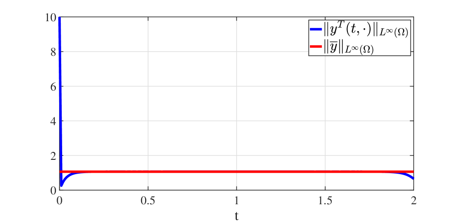
Figure 4. graph of the function $t\longrightarrow\|y^{T}(t)\|_{{\rm L}^{\infty}\left(\Omega\right)}$ (in blue) and $\|\overline{y}\|_{{\rm L}^{\infty}\left(\Omega\right)}$ (in red), where $y^{T}$ denotes an optimal state, whereas $\overline{y}$ stands for an optimal steady state.

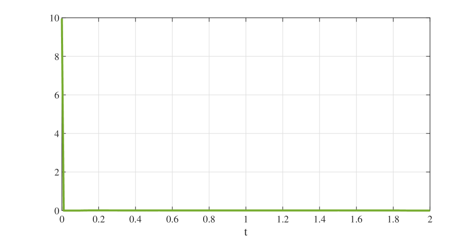
Figure 5. graph of the function $t\longrightarrow\left\|y^{T}(t)-\overline{y}\right\|_{{\rm L}^{\infty}\left(\Omega\right)}$, where $y^{T}$ denotes an optimal state, whereas $\overline{y}$ stands for an optimal steady state.

4. Conclusions and open problems

In this manuscript we have obtained some global turnpike results for an optimal control problem governed by a nonlinear state equation. For any data and small targets, we have shown that the exponential turnpike property holds (0.1). For arbitrary targets, we have proved the convergence of averages (0.4), under the added assumption of controlling everywhere. One of the main tools employed for our analysis is an ${\rm L}^{\infty}$ bound of the norm of the optima, uniform in the time horizon (Lemma 1.1). Numerical simulation have been performed, which confirms the theoretical results.

We present now some interesting open problems in the field.

4.1. General targets with any control domain

In 0.4 we have proved the convergence of averages for large targets, in the context of control everywhere. An interesting challenge is to prove the exponential turnpike property, even if the control is local (namely $\omega\subsetneq\Omega$). The challenge is to prove the following conjecture.

Conjecture 4.1.

Consider the control problem 2-1. Take any initial datum $y_{0}\in{\rm L}^{\infty}\left(\Omega\right)$ and any target $z\in{\rm L}^{\infty}(\omega_{0})$. Let $u^{T}$ be a minimizer of 1. There exists an optimal pair $(\overline{u},\overline{y})$ for 5-4 such that

$$\|u^{T}(t)-\overline{u}\|_{{\rm L}^{\infty}\left(\omega\right)}+\|y^{T}(t)-\overline{y}\|_{{\rm L}^{\infty}\left(\Omega\right)}\leq K\left[\exp\left(-\mu t\right)+\exp\left(-\mu(T-t)\right)\right],\hskip 17.07182pt\forall t\in[0,T],$$ (60)

the constants $K$ and $\mu>0$ being independent of the time horizon $T$.

In [36] special large targets $z$ are constructed, such that the optimal control for the steady problem 5-4 is not unique. For those targets, a question arises: if the turnpike property is satisfied, which minimizer for 5-4 attracts the optimal solutions to 2-1?
Note that, in the context of internal control, the counterexample to uniqueness in [36] is valid in case of local control $\omega\subsetneq\Omega$.

Generally speaking a further investigation is required for the linearized optimality system determined in [40, subsection 3.1]. We introduce the problem. As in 3, consider the optimality system for 2-1

$$\begin{cases}y^{T}_{t}-\Delta y^{T}+f(y^{T})=-q^{T}\chi_{\omega}\hskip 79.6678pt&\mbox{in}\hskip 2.84544pt(0,T)\times\Omega\\ y^{T}=0&\mbox{on}\hskip 2.84544pt(0,T)\times\partial\Omega\\ y^{T}(0,x)=y_{0}(x)&\mbox{in}\hskip 2.84544pt\Omega\\ -q^{T}_{t}-\Delta q^{T}+f^{\prime}(y^{T})q^{T}=\beta(y^{T}-z)\chi_{\omega_{0}}\hskip 79.6678pt&\mbox{in}\hskip 2.84544pt(0,T)\times\Omega\\ q^{T}=0&\mbox{on}\hskip 2.84544pt(0,T)\times\partial\Omega\\ q^{T}(T,x)=0&\mbox{in}\hskip 2.84544pt\Omega.\\ \end{cases}$$ (61)

Pick any optimal pair $(\overline{u},\overline{y})$ for 5-4. By the first order optimality conditions, the steady optimal control reads as $\overline{u}=-\overline{q}\chi_{\omega}$, with

$$\begin{cases}-\Delta\overline{y}+f(\overline{y})=-\overline{q}\chi_{\omega}\hskip 79.6678pt&\mbox{in}\hskip 2.84544pt\Omega\\ \overline{y}=0&\mbox{on}\hskip 2.84544pt\partial\Omega\\ -\Delta\overline{q}+f^{\prime}(\overline{y})\overline{q}=\beta(\overline{y}-z)\chi_{\omega_{0}}\hskip 79.6678pt&\mbox{in}\hskip 2.84544pt\Omega\\ \overline{q}=0&\mbox{on}\hskip 2.84544pt\partial\Omega.\end{cases}$$ (62)

As in [40], we introduce the perturbation variables

$$\eta^{T}\coloneqq y^{T}-\overline{y}\hskip 8.5359pt\mbox{and}\hskip 8.5359pt\varphi^{T}\coloneqq q^{T}-\overline{q}$$ (63)

and we write down the linearized optimality system around $(\overline{u},\overline{y})$

$$\begin{cases}\eta^{T}_{t}-\Delta\eta^{T}+f^{\prime}(\overline{y})\eta^{T}=-\varphi^{T}\chi_{\omega}\hskip 79.6678pt&\mbox{in}\hskip 2.84544pt(0,T)\times\Omega\\ \eta^{T}=0&\mbox{on}\hskip 2.84544pt(0,T)\times\partial\Omega\\ \eta^{T}(0,x)=y_{0}(x)-\overline{y}(x)&\mbox{in}\hskip 2.84544pt\Omega\\ -\varphi^{T}_{t}-\Delta\varphi^{T}+f^{\prime}(\overline{y})\varphi^{T}=\left(\beta\chi_{\omega_{0}}-f^{\prime\prime}\left(\overline{y}\right)\overline{q}\right)\eta^{T}\hskip 79.6678pt&\mbox{in}\hskip 2.84544pt(0,T)\times\Omega\\ \varphi^{T}=0&\mbox{on}\hskip 2.84544pt(0,T)\times\partial\Omega\\ \varphi^{T}(T,x)=-\overline{q}(x)&\mbox{in}\hskip 2.84544pt\Omega.\\ \end{cases}$$ (64)

As pointed out in [40, Theorem 1 in subsection 3.1], a key point is to check the validity of the turnpike property for the linearized optimality system 64. This is complicated because of the term $\beta\chi_{\omega_{0}}-f^{\prime\prime}\left(\overline{y}\right)\overline{q}$, whose sign is unknown for general large targets. Furthermore, in case of nonuniqueness of steady optimum, it would be interesting to compute the spectrum of the linearized system around any steady optima to check if among them one is a better attractor.

We conclude this subsection observing that, even in case the control acts everywhere ($\omega=\Omega$), theory is not conclusive. Indeed, our results (Theorem 0.4 and Lemma 2.3) provides information on the performances of the steady controls and the estimate of the ${\rm L}^{2}$ norm of the time derivative of the optimal state. The proof of Conjecture 4.1 in this case would require the use of Hamilton-Jacobi techniques (see e.g. [7, Theorem 7.4.17]) to carry over our results to the optimal control and states by a feedback operator.

4.2. Different nonlinear state equations

It would be interesting to check the validity of the turnpike property, for different state equations, e.g. hyperbolic PDEs. This has been done in the linear case [39, 58, 24]. To address the nonlinear case the scheme we have employed can be used (uniform estimates for the optima, linearization and global-local argument). However, appropriate modifications have to be made to the proofs according to regularity properties of the state equation.

Appendix A Parabolic regularity results

One of the key tool to carry on the proof of Lemma 1.1 is the following regularity result.

Lemma A.1.

Let $\Omega$ be a bounded open set of $\mathbb{R}^{n}$, $n\in\left\{1,2,3\right\}$, with ${\rm C}^{2}$ boundary. Let $c:(0,T)\times\Omega\longrightarrow\mathbb{R}$ be measurable and nonnegative. Let $y_{0}\in{\rm L}^{\infty}\left(\Omega\right)$ be an initial datum and let $h\in{\rm L}^{2}((0,T)\times\Omega)$ be a source term. Let $y$ be the solution to

$$\begin{dcases}y_{t}-\Delta y+cy=h\hskip 79.6678pt&\mbox{in}\hskip 2.84544pt(0,T)\times\Omega\\ y=0&\mbox{on}\hskip 2.84544pt(0,T)\times\partial\Omega\\ y(0,x)=y_{0}(x)&\mbox{in}\hskip 2.84544pt\Omega.\\ \end{dcases}$$

Choose $y_{0}$ and $h$ so that $cy\in{\rm L}^{2}\left(\left(0,T\right)\times\Omega\right)$. Then, $y\in{\rm L}^{2}\left((0,T);{\rm L}^{\infty}\left(\Omega\right)\right)$ and we have

$$\|y\|_{{\rm L}^{2}\left((0,T);{\rm L}^{\infty}\left(\Omega\right)\right)}\leq K\left[\|y_{0}\|_{{\rm L}^{\infty}\left(\Omega\right)}+\|h\|_{{\rm L}^{2}\left(\left(0,T\right)\times\Omega\right)}\right],$$ (65)

where $K=K\left(\Omega\right)$.

Proof of Lemma A.1..

Step 1  Comparison
Let $\psi$ be the solution to:

$$\begin{dcases}\psi_{t}-\Delta\psi=|h|\hskip 17.07182pt&\mbox{in}\hskip 2.84544pt(0,T)\times\Omega\\ \psi=0&\mbox{on}\hskip 2.84544pt(0,T)\times\partial\Omega\\ \psi(0,x)=|y_{0}|.&\mbox{in}\hskip 2.84544pt\Omega\\ \end{dcases}$$ (66)

Since $c\geq 0$, a.e. in $(0,T)\times\Omega$, by a comparison argument, for each $t\in[0,T]$:

$$|y(t,x)|\leq\psi(t,x),\quad\mbox{a.e. }x\in\Omega.$$ (67)

Now, since $y_{0}$ and $h$ are bounded, again by comparison principle applied to 66, $\psi$ is bounded. Hence, by 67, $y$ is bounded as well and

$$\int_{0}^{T}\|y(t)\|_{{\rm L}^{\infty}\left(\Omega\right)}^{2}dt\leq\int_{0}^{T}\|\psi(t)\|_{{\rm L}^{\infty}\left(\Omega\right)}^{2}dt.$$ (68)

Then, to conclude it suffices to show

$$\|\psi\|_{{\rm L}^{2}(0,T;{\rm L}^{\infty}\left(\Omega\right))}\leq K\left[\|y_{0}\|_{{\rm L}^{\infty}\left(\Omega\right)}+\|h\|_{{\rm L}^{2}((0,T)\times\Omega)}\right],$$

the constant $K$ being independent of $T$.
Step 2  Splitting
Split $\psi=\xi+\chi$, where $\xi$ solves:

$$\begin{dcases}\xi_{t}-\Delta\xi=0\hskip 17.07182pt&\mbox{in}\hskip 2.84544pt(0,T)\times\Omega\\ \xi=0&\mbox{on}\hskip 2.84544pt(0,T)\times\partial\Omega\\ \xi(0,x)=|y_{0}|&\mbox{in}\hskip 2.84544pt\Omega\\ \end{dcases}$$ (69)

while $\chi$ satisfies:

$$\begin{dcases}\chi_{t}-\Delta\chi=|h|\hskip 17.07182pt&\mbox{in}\hskip 2.84544pt(0,T)\times\Omega\\ \chi=0&\mbox{on}\hskip 2.84544pt(0,T)\times\partial\Omega\\ \chi(0,x)=0&\mbox{in}\hskip 2.84544pt\Omega.\\ \end{dcases}$$ (70)

First of all, we prove an estimate like 65 for $\xi$. We start by employing maximum principle (see [41]) to 68, getting

$$\|\xi\|_{{\rm L}^{\infty}\left((0,T)\times\Omega\right)}\leq\|y_{0}\|_{{\rm L}^{\infty}\left(\Omega\right)}.$$ (71)

Now, if $T\geq 1$, by the regularizing effect and the exponential stability of the heat equation, for any $t\in[1,T]$, we have

$$\|\xi(t)\|_{{\rm L}^{\infty}\left(\Omega\right)}\leq K\|\xi(t-1)\|_{{\rm L}^{2}\left(\Omega\right)}\leq K\exp\left(-\lambda_{1}(t-1)\right)\|y_{0}\|_{{\rm L}^{2}\left(\Omega\right)},$$ (72)

the constant $K$ depending only on the domain $\Omega$. Then, by 71 and 72, for any $T>0$, for every $t\in[0,T]$,

$$\|\xi(t)\|_{{\rm L}^{\infty}\left(\Omega\right)}\leq K\min\left\{1,\exp\left(-\lambda_{1}(t-1)\right)\right\}\|y_{0}\|_{{\rm L}^{\infty}\left(\Omega\right)},$$ (73)

with $K=K\left(\Omega\right)$.

Now, we focus on 70. By parabolic regularity (see e.g. [18, Theorem 5 subsection 7.1.3]), $\chi\in{\rm L}^{2}(0,T;{\rm H}^{2}\left(\Omega\right))$, with $\chi_{t}\in{\rm L}^{2}((0,T)\times\Omega)$. Then, by multiplying 70 by $-\Delta\chi$ and integrating over $[0,T]\times\Omega$, we obtain

$$\frac{1}{2}\|\nabla\chi(T)\|_{{\rm L}^{2}\left(\Omega\right)}^{2}+\int_{0}^{T}\int_{\Omega}|\Delta\chi|^{2}dxdt\leq\|h\|_{{\rm L}^{2}\left((0,T)\times\Omega\right)}\|\Delta\chi\|_{{\rm L}^{2}\left((0,T)\times\Omega\right)}.$$

By Young’s Inequality,

$$\int_{0}^{T}\int_{\Omega}|\Delta\chi|^{2}dxdt\leq\frac{1}{2}\|h\|_{{\rm L}^{2}\left((0,T)\times\Omega\right)}^{2}+\frac{1}{2}\|\Delta\chi\|_{{\rm L}^{2}\left((0,T)\times\Omega\right)}^{2},$$

which leads to

$$\int_{0}^{T}\int_{\Omega}|\Delta\chi|^{2}dxdt\leq\|h\|_{{\rm L}^{2}\left((0,T)\times\Omega\right)}^{2}.$$

Now, by [18, Theorem 6 subsection 5.6.3] and [18, Theorem 4 subsection 6.3.2],

$$\int_{0}^{T}\|\chi\|_{{\rm L}^{\infty}\left(\Omega\right)}^{2}dt\leq K\int_{0}^{T}\|\chi\|_{{\rm H}^{2}\left(\Omega\right)}^{2}dt\leq K\int_{0}^{T}\int_{\Omega}|\Delta\chi|^{2}dxdt\leq K\|h\|_{{\rm L}^{2}\left((0,T)\times\Omega\right)}^{2}.$$ (74)

Finally, by 68, 73 and 74,

$$\int_{0}^{T}\|y\|_{{\rm L}^{\infty}\left(\Omega\right)}^{2}dt\leq 2\int_{0}^{T}\|\xi\|_{{\rm L}^{\infty}\left(\Omega\right)}^{2}dt+2K\int_{0}^{T}\|\chi\|_{{\rm L}^{\infty}\left(\Omega\right)}^{2}dt\leq K\left[\|y_{0}\|_{{\rm L}^{\infty}\left(\Omega\right)}^{2}+\|h\|_{{\rm L}^{2}\left((0,T)\times\Omega\right)}^{2}\right],$$

as required. ∎

The following regularity result is employed in the proof of Lemma 1.1.

Lemma A.2.

Let $\Omega\subset\mathbb{R}^{n}$ be a bounded open set, with $\partial\Omega\in{\rm C}^{\infty}$. Let $c\in{\rm L}^{\infty}((0,T)\times\Omega)$ be nonnegative. Let $y_{0}\in{\rm L}^{\infty}\left(\Omega\right)$ an initial datum and $h\in{\rm L}^{\infty}((0,T)\times\Omega)$ a source term. Let $\overline{T}\in(0,T)$ and set $N\coloneqq\left\lfloor{T/\overline{T}}\right\rfloor$. Let $y$ be the solution to

$$\begin{dcases}y_{t}-\Delta y+cy=h\hskip 79.6678pt&\mbox{in}\hskip 2.84544pt(0,T)\times\Omega\\ y=0&\mbox{on}\hskip 2.84544pt(0,T)\times\partial\Omega\\ y(0,x)=y_{0}(x)&\mbox{in}\hskip 2.84544pt\Omega.\\ \end{dcases}$$

Then, $y\in{\rm L}^{\infty}((0,T)\times\Omega)$ and we have

$$\|y\|_{{\rm L}^{\infty}((0,T)\times\Omega)}\leq K\left[\|y_{0}\|_{{\rm L}^{\infty}\left(\Omega\right)}+\max_{i=1,\dots,N}\|h\|_{{\rm L}^{2}(((i-1)\overline{T},i\overline{T});{\rm L}^{\infty}\left(\Omega\right))}+\|h\|_{{\rm L}^{2}(N\overline{T},T;{\rm L}^{\infty}\left(\Omega\right))}\right],$$ (75)

where $K=K\left(\Omega,\overline{T}\right)$ is independent of the potential $c\geq 0$ and the time horizon $T$.

Proof of Lemma A.2.

Step 1  Comparison argument
Let $\psi$ be the solution to:

$$\begin{dcases}\psi_{t}-\Delta\psi=|h|\hskip 17.07182pt&\mbox{in}\hskip 2.84544pt(0,T)\times\Omega\\ \psi=0&\mbox{on}\hskip 2.84544pt(0,T)\times\partial\Omega\\ \psi(0,x)=|y_{0}|.&\mbox{in}\hskip 2.84544pt\Omega\\ \end{dcases}$$ (76)

Since $c\geq 0$, a.e. in $(0,T)\times\Omega$, by a comparison argument, for each $t\in[0,T]$:

$$|y(t,x)|\leq\psi(t,x),\quad\mbox{a.e. }x\in\Omega.$$ (77)

Now, since $y_{0}$ and $h$ are bounded, again by comparison principle applied to 76, $\psi$ is bounded. Hence, by 77, $y$ is bounded as well and

$$\|y\|_{{\rm L}^{\infty}((0,T)\times\Omega)}\leq\|\psi\|_{{\rm L}^{\infty}((0,T)\times\Omega)}.$$ (78)

Then, to conclude it suffices to show

$$\|\psi\|_{{\rm L}^{\infty}((0,T)\times\Omega)}\leq K\left[\|y_{0}\|_{{\rm L}^{\infty}\left(\Omega\right)}+\max_{i=1,\dots,N}\|h\|_{{\rm L}^{2}(((i-1)\overline{T},i\overline{T});{\rm L}^{\infty}\left(\Omega\right))}+\|h\|_{{\rm L}^{2}(N\overline{T},T;{\rm L}^{\infty}\left(\Omega\right))}\right],$$

the constant $K=K\left(\Omega,\overline{T}\right)$ being independent of $T$.
Step 2   Conclusion
Let $\left\{S(t)\right\}_{t\in\mathbb{R}^{+}}$ be the heat semigroup on $\Omega$, with zero Dirichlet boundary conditions. Fix $\varepsilon\in(0,\overline{T})$. By the regularizing effect of the heat equation (see, e.g. [6, Theorem 10.1, section 10.1]), for any $t\geq\varepsilon$,

$$\|S(t)y_{0}\|_{{\rm L}^{\infty}\left(\Omega\right)}\leq K\exp(-\mu(t-\varepsilon))\|y_{0}\|_{{\rm L}^{2}\left(\Omega\right)}\leq K\exp(-\mu(t-\varepsilon))\|y_{0}\|_{{\rm L}^{\infty}\left(\Omega\right)}.$$

For $t\in[0,\varepsilon]$, by comparison principle, we have

$$\|S(t)y_{0}\|_{{\rm L}^{\infty}\left(\Omega\right)}\leq K\|y_{0}\|_{{\rm L}^{\infty}\left(\Omega\right)}\leq K\exp(-\mu(t-\varepsilon))\|y_{0}\|_{{\rm L}^{\infty}\left(\Omega\right)},$$

being $\exp(-\mu(t-\varepsilon))\geq 1$. Hence, for any $t\geq 0$,

$$\|S(t)y_{0}\|_{{\rm L}^{\infty}\left(\Omega\right)}\leq K\exp(-\mu(t-\varepsilon))\|y_{0}\|_{{\rm L}^{\infty}\left(\Omega\right)}.$$ (79)

Then, by the Duhamel formula, for any $t\in[0,T]$, we have

$$\psi(t)=S(t)\left(|y_{0}|\right)+\int_{0}^{t}S(t-s)\left(|h(s)|\right)ds.$$ (80)

Now, by 79, for any $t\geq 0$,

$$\|S(t)\left(|y_{0}|\right)\|_{{\rm L}^{\infty}\left(\Omega\right)}\leq K\exp\left(-\mu(t-\varepsilon)\right)\|y_{0}\|_{{\rm L}^{\infty}\left(\Omega\right)}.$$ (81)

Besides, by applying 79 to the integral term $\eta(t)\coloneqq\int_{0}^{t}S(t-s)\left(|h(s)|\right)ds$ in 80, we obtain

$$\|\eta(t)\|_{{\rm L}^{\infty}} \leq \int_{0}^{t}\|S(t-s)\left(|h(s)|\right)\|_{{\rm L}^{\infty}}ds$$ (82)

$$\leq K\int_{0}^{t}\exp(-\mu(t-s-\varepsilon))\|h(s)\|_{{\rm L}^{\infty}}ds$$

$$\leq K\left[\sum_{i=1}^{\left\lfloor{\frac{t}{\overline{T}}}\right\rfloor}\exp(-\mu(t-\varepsilon-i\overline{T}))\int_{(i-1)\overline{T}}^{i\overline{T}}\exp(-\mu(i\overline{T}-s))\|h(s)\|_{{\rm L}^{\infty}}ds\right.$$

$$\left.+\int_{\left(\left\lfloor{\frac{t}{\overline{T}}}\right\rfloor-1\right)\overline{T}}^{t}\exp(-\mu(t-s-\varepsilon))\|h(s)\|_{{\rm L}^{\infty}}ds\right]$$

$$\leq K\left\{\sum_{i=1}^{\left\lfloor{\frac{t}{\overline{T}}}\right\rfloor}\exp(-\mu(t-\varepsilon-i\overline{T}))\left[\int_{(i-1)\overline{T}}^{i\overline{T}}\exp(-2\mu(i\overline{T}-s))ds\right]^{\frac{1}{2}}\left[\int_{(i-1)\overline{T}}^{i\overline{T}}\|h(s)\|_{{\rm L}^{\infty}}^{2}ds\right]^{\frac{1}{2}}\right.$$

$$\left.+\left[\int_{\left(\left\lfloor{\frac{t}{\overline{T}}}\right\rfloor-1\right)\overline{T}}^{t}\exp(-2\mu(t-s-\varepsilon))ds\right]^{\frac{1}{2}}\left[\int_{\left(\left\lfloor{\frac{t}{\overline{T}}}\right\rfloor-1\right)\overline{T}}^{t}\|h(s)\|_{{\rm L}^{\infty}}^{2}ds\right]^{\frac{1}{2}}\right\}$$

$$\leq K\left[\sum_{i=1}^{\left\lfloor{\frac{t}{\overline{T}}}\right\rfloor}\exp(-\mu(t-\varepsilon-i\overline{T}))\|h\|_{{\rm L}^{2}((i-1)\overline{T},i\overline{T};{\rm L}^{\infty}\left(\Omega\right))}\right.$$

$$\left.+\|h\|_{{\rm L}^{2}(N\overline{T},T;{\rm L}^{\infty}\left(\Omega\right))}\right]$$

$$\leq K\left[\sum_{i=1}^{\left\lfloor{\frac{t}{\overline{T}}}\right\rfloor}\exp(-\mu(t-\varepsilon-i\overline{T}))\max_{i=1,\dots,N}\|h\|_{{\rm L}^{2}(((i-1)\overline{T},i\overline{T});{\rm L}^{\infty}\left(\Omega\right))}\right.$$

$$\left.+\|h\|_{{\rm L}^{2}(N\overline{T},T;{\rm L}^{\infty}\left(\Omega\right))}\right].$$

Now, the sum

$$\sum_{i=1}^{\left\lfloor{\frac{t}{\overline{T}}}\right\rfloor}\exp(-\mu(t-\varepsilon-i\overline{T})) \leq\exp(\mu\varepsilon)\sum_{i=1}^{\left\lfloor{\frac{t}{\overline{T}}}\right\rfloor}\exp\left(-\mu\left(\left\lfloor{\frac{t}{\overline{T}}}\right\rfloor\overline{T}-i\overline{T}\right)\right)$$

$$=\exp(\mu\varepsilon)\sum_{i=1}^{\left\lfloor{\frac{t}{\overline{T}}}\right\rfloor}\exp\left(-\mu\left(\left\lfloor{\frac{t}{\overline{T}}}\right\rfloor-i\right)\overline{T}\right)$$ (83)

$$=\exp(\mu\varepsilon)\sum_{j=0}^{\left\lfloor{\frac{t}{\overline{T}}}\right\rfloor-1}\exp\left(-\mu j\overline{T}\right)$$ (84)

$$\leq\exp(\mu\varepsilon)\sum_{j=0}^{+\infty}\exp\left(-\mu j\overline{T}\right)$$ (85)

$$=\frac{\exp(\mu\varepsilon)}{1-\exp\left(-\mu\overline{T}\right)},$$ (86)

where in (83) we have used $t\leq\left\lfloor{\frac{t}{\overline{T}}}\right\rfloor$, in (84) we have performed the change of variable $j\coloneqq\left\lfloor{\frac{t}{\overline{T}}}\right\rfloor-i$ and in (86) we have computed the geometric series. Hence, by (82) and the above computation, we have

$$\|\eta(t)\|_{{\rm L}^{\infty}} \leq K\left[\sum_{i=1}^{\left\lfloor{\frac{t}{\overline{T}}}\right\rfloor}\exp(-\mu(t-\varepsilon-i\overline{T}))\|h\|_{{\rm L}^{2}((i-1)\overline{T},i\overline{T};{\rm L}^{\infty}\left(\Omega\right))}\right.$$ (88)

$$\left.+\|h\|_{{\rm L}^{2}(N\overline{T},T;{\rm L}^{\infty}\left(\Omega\right))}\right]$$

$$\leq K\left[\frac{\exp(\mu\varepsilon)}{1-\exp\left(-\mu\overline{T}\right)}\max_{i=1,\dots,N}\|h\|_{{\rm L}^{2}(((i-1)\overline{T},i\overline{T});{\rm L}^{\infty}\left(\Omega\right))}\right.$$

$$\left.+\|h\|_{{\rm L}^{2}(N\overline{T},T;{\rm L}^{\infty}\left(\Omega\right))}\right]$$

$$\leq K\left[\max_{i=1,\dots,N}\|h\|_{{\rm L}^{2}((i-1)\overline{T},i\overline{T};{\rm L}^{\infty}\left(\Omega\right))}+\|h\|_{{\rm L}^{2}(N\overline{T},T;{\rm L}^{\infty}\left(\Omega\right))}\right],$$

with $K=K\left(\Omega,\overline{T}\right)$

Then, by 81 and 82, for each $t\in[0,T]$

$$\|\psi(t)\|_{{\rm L}^{\infty}\left(\Omega\right)}\leq K\exp\left(-\mu(t-\varepsilon)\right)\left[\|y_{0}\|_{{\rm L}^{\infty}\left(\Omega\right)}+\max_{i=1,\dots,N}\|h\|_{{\rm L}^{2}((i-1)\overline{T},i\overline{T};{\rm L}^{\infty}\left(\Omega\right))}+\|h\|_{{\rm L}^{2}(N\overline{T},T;{\rm L}^{\infty}\left(\Omega\right))}\right]$$

as desired. ∎

Appendix B Well posedeness and regularity of the state equation

In this subsection we study the well posedeness and regularity properties of the state equation (2).

Let $\Omega$ be a bounded open subset of $\mathbb{R}^{n}$, with boundary $\partial\Omega\in C^{2}$. The nonlinearity $f\in{\rm C}^{1}(\mathbb{R})$ is nondecreasing and $f(0)=0$. Let us also mention that, among the equivalent definitions for ${\rm H}^{1}_{0}$ norm, we choose $\left\|y\right\|_{{\rm H}^{1}_{0}\left(\Omega\right)}\coloneqq\sqrt{\int_{\Omega}\left\|\nabla y\right\|^{2}dx}$ as suggested by Poincaré’s inequality [6, Corollary 9.19 page 290]. To define the notion of solution, we introduce the class of test functions

$$\mathscr{C}\coloneqq{\rm L}^{2}\left(\left(0,T\right);{\rm H}^{1}_{0}\left(\Omega\right)\right)\cap{\rm L}^{\infty}\left(\left(0,T\right)\times\Omega\right),$$

the Hilbert space (see e.g. [35, (1.8)-(1.9) page 102])

$$W\left(0,T\right)\coloneqq\left\{y\in{\rm L}^{2}\left(\left(0,T\right);{\rm H}^{1}_{0}\left(\Omega\right)\right)\ |\ y_{t}\in{\rm L}^{2}\left(\left(0,T\right);{\rm H}^{-1}\left(\Omega\right)\right)\right\}$$

endowed with the norm

$$\left\|y\right\|_{W\left(0,T\right)}\coloneqq\left\|y\right\|_{{\rm L}^{2}\left(\left(0,T\right);{\rm H}^{1}_{0}\left(\Omega\right)\right)}+\|y_{t}\|_{{\rm L}^{2}\left(\left(0,T\right);{\rm H}^{-1}\left(\Omega\right)\right)}.$$

and the Hilbert space

$$W_{R}\left(0,T\right)\coloneqq\left\{y\in{\rm L}^{2}((0,T);{\rm H}^{1}_{0}\left(\Omega\right)\cap{\rm H}^{2}\left(\Omega\right))\ |\ y_{t}\in{\rm L}^{2}\left(\left(0,T\right)\times\Omega\right)\right\}$$ (89)

endowed with the norm:

$$\|y\|_{W_{R}\left(0,T\right)}\coloneqq\|y\|_{{\rm L}^{2}((0,T);{\rm H}^{2}\left(\Omega\right))}+\|y_{t}\|_{{\rm L}^{2}\left(\left(0,T\right)\times\Omega\right)}.$$

Definition B.1.

Let $y_{0}\in{\rm L}^{\infty}\left(\Omega\right)$ and $h\in{\rm L}^{2}\left(\left(0,T\right)\times\Omega\right)$. Then, $y\in W\left(0,T\right)$ is said to be a solution to the Cauchy problem

$$\begin{dcases}y_{t}-\Delta y+f\left(y\right)=h\hskip 79.6678pt&\mbox{in}\hskip 2.84544pt(0,T)\times\Omega\\ y=0&\mbox{on}\hskip 2.84544pt(0,T)\times\partial\Omega\\ y(0,x)=y_{0}(x)&\mbox{in}\hskip 2.84544pt\Omega.\end{dcases}$$ (90)

if $y\left(0,\cdot\right)=y_{0}$ in ${\rm L}^{2}\left(\Omega\right)$, $f\left(y\right)\in{\rm L}^{1}\left(\left(0,T\right)\times\Omega\right)$ and for any test function $\varphi\in\mathscr{C}$, we have

$$\int_{0}^{T}\left\{\langle y_{t},\varphi\rangle+\int_{\Omega}\left[\nabla y\nabla\varphi+f\left(y\right)\varphi\right]dx\right\}dt=\int_{0}^{T}\int_{\Omega}h\varphi dxdt,$$ (91)

where $\langle\cdot,\cdot\rangle$ denotes the duality product $\left({\rm H}^{1}_{0}\left(\Omega\right),{\rm H}^{-1}\left(\Omega\right)\right)$.

To state the next Proposition, we introduce the following class of initial data

$${\rm L}_{1,{\rm F}}^{2}\coloneqq\left\{y_{0}\in{\rm L}^{2}\left(\Omega\right)\ |\ F\left(y_{0}\right)\in{\rm L}^{1}\left(\Omega\right)\right\},$$ (92)

where $F\left(y\right)\coloneqq\int_{0}^{y}f\left(\xi\right)d\xi$. Next Proposition is devoted to the well posedeness of (90), while Proposition B.4 deals with regularity properties.

Proposition B.2 (Well posedeness).

Let $y_{0}\in{\rm L}_{1,{\rm F}}^{2}$ be an initial datum and $h\in{\rm L}^{2}\left(\left(0,T\right)\times\Omega\right)$ be a source term. There exists a unique solution $y$ to (90). Moreover, $f\left(y\right)$ is square integrable, i.e. $f\left(y\right)\in{\rm L}^{2}\left(\left(0,T\right)\times\Omega\right)$, with estimates

$$\|y\|_{{\rm L}^{2}\left(\left(0,T\right);{\rm H}^{1}_{0}\left(\Omega\right)\right)}\leq\|y_{0}\|_{{\rm L}^{2}\left(\Omega\right)}+\|h\|_{{\rm L}^{2}\left(\left(0,T\right);{\rm H}^{-1}\left(\Omega\right)\right)},$$ (93)

$$\left\|f\left(y\right)\right\|_{{\rm L}^{2}\left(\left(0,T\right)\times\Omega\right)}\leq\sqrt{2\left\|F\left(y_{0}\right)\right\|_{{\rm L}^{1}\left(\Omega\right)}}+\|h\|_{{\rm L}^{2}\left(\left(0,T\right)\times\Omega\right)}$$ (94)

and

$$\left\|y_{t}\right\|_{{\rm L}^{2}\left(\left(0,T\right);{\rm H}^{-1}\left(\Omega\right)\right)}\leq K\left[\left\|y_{0}\right\|_{{\rm L}^{2}\left(\Omega\right)}+\sqrt{\left\|F\left(y_{0}\right)\right\|_{{\rm L}^{1}\left(\Omega\right)}}+\|h\|_{{\rm L}^{2}\left(\left(0,T\right)\times\Omega\right)}\right],$$ (95)

where $F\left(y\right)=\int_{0}^{y}f\left(\xi\right)d\xi$ and $K=K\left(\Omega\right)$.

Remark B.3.

In the literature, well posedeness and regularity of dissipative semilinear heat equations have been treated extensively (see e.g. [11, 44, 4]). However, in [11, 44] the source is required to be ${\rm L}^{p}$, with $p$ large enough to have bounded solutions. Our goal is to show how to prove well posedeness and regularity with ${\rm L}^{2}$ source. As we shall see in Proposition B.4, if the initial datum is bounded, the solution is bounded in space (of class ${\rm L}^{2}\left(\left(0,T\right);{\rm L}^{\infty}\left(\Omega\right)\right)$), but possibly unbounded in space-time. In [4, Proposition 5.1 page 195] unbounded sources are considered, but to have solutions in $W\left(0,T\right)$ the initial datum is supposed to be in ${\rm H}^{1}_{0}\left(\Omega\right)\cap{\rm L}_{1,{\rm F}}^{2}$. In our result, we ask only $y_{0}\in{\rm L}_{1,{\rm F}}^{2}$. Note that, in case the source is only space dependent $h=h(x)$, (90) can be seen as a gradient flow of the convex functional

$$I:D(I)\subset{\rm L}^{2}\left(\Omega\right)\longrightarrow\mathbb{R},\hskip 8.5359ptI\left(y\right)\coloneqq\int_{\Omega}\left[\frac{1}{2}\left\|\nabla y\right\|^{2}+F\left(y\right)-hy\right]dx,$$ (96)

where $F\left(y\right)=\int_{0}^{y}f\left(\xi\right)d\xi$ (see [18, section 9.6] and references therein). This explains the condition $F\left(y_{0}\right)\in{\rm L}^{1}\left(\Omega\right)$ we imposed, which requires that the term $\int_{\Omega}F\left(y_{0}\right)dx$ appearing in the functional (96) is finite.

The initial datum $y_{0}$ is supposed to be in ${\rm L}_{1,{\rm F}}^{2}$. However, this condition may be relaxed to weaker integrability conditions by looking for a solution in a larger Banach space.

The proof of Proposition B.2 is inspired by [5, Theorem 4.7, page 29].

Proof of Proposition B.2..

Uniqueness follows from energy estimates. We focus on the proof of existence and estimates. Along the proof, we will use that $f$ is nondecreasing and $f(0)=0$, which yield $f^{\prime}(y)\geq 0$ and $F\left(y\right)=\int_{0}^{y}f\left(\xi\right)d\xi\geq 0$, for any $y\in\mathbb{R}$. Integration by parts will be employed. We will denote by $K$ a large enough constant depending only on the domain $\Omega$.

Step 1  Existence for bounded data
Take initial datum $y_{0}\in{\rm L}^{\infty}(\Omega)$ and source $h\in{\rm L}^{\infty}((0,T)\times\Omega)$. By [11, Theorem 2.1 page 547], there exists a bounded solution $y$ to (90). Truncation methods are employed to deal with possibly non Lipschitz nonlinearity.

Step 2  Estimates for bounded data
We now aim at proving (93), (94) and (95) for ${\rm L}^{\infty}$ data. In order to show (93), in (91) let us choose as test function $\varphi\coloneqq y$, getting

$$\int_{0}^{T}\int_{\Omega}hydxdt = \int_{0}^{T}\int_{\Omega}\left[y_{t}y+\left\|\nabla y\right\|^{2}+f\left(y\right)y\right]dxdt$$

$$= \frac{1}{2}\left[\left\|y(T,\cdot)\right\|_{{\rm L}^{2}(\Omega)}^{2}-\left\|y_{0}\right\|_{{\rm L}^{2}(\Omega)}^{2}\right]+\|y\|_{{\rm L}^{2}\left(\left(0,T\right);{\rm H}^{1}_{0}\left(\Omega\right)\right)}^{2}+\int_{0}^{T}\int_{\Omega}f\left(y\right)ydxdt.$$

Then, by Young’s inequality

$$\|y\|_{{\rm L}^{2}\left(\left(0,T\right);{\rm H}^{1}_{0}\left(\Omega\right)\right)}^{2}+\int_{0}^{T}\int_{\Omega}f\left(y\right)ydxdt \leq \int_{0}^{T}\int_{\Omega}hydxdt+\left\|y_{0}\right\|_{{\rm L}^{2}(\Omega)}^{2}$$

$$\leq \frac{1}{2}\left\|h\right\|_{{\rm L}^{2}\left(\left(0,T\right);{\rm H}^{-1}\left(\Omega\right)\right)}^{2}+\frac{1}{2}\left\|y\right\|_{{\rm L}^{2}\left(\left(0,T\right);{\rm H}^{1}_{0}\left(\Omega\right)\right)}^{2}+\frac{1}{2}\left\|y_{0}\right\|_{{\rm L}^{2}(\Omega)}^{2},$$

which yields

$$\frac{1}{2}\|y\|_{{\rm L}^{2}\left(\left(0,T\right);{\rm H}^{1}_{0}\left(\Omega\right)\right)}^{2}+\int_{0}^{T}\int_{\Omega}f\left(y\right)ydxdt\leq\frac{1}{2}\left\|h\right\|_{{\rm L}^{2}\left(\left(0,T\right);{\rm H}^{-1}\left(\Omega\right)\right)}^{2}+\frac{1}{2}\left\|y_{0}\right\|_{{\rm L}^{2}(\Omega)}^{2},$$ (99)

whence (93) follows. For the proof of (94), let us observe that, since $y$ is bounded and $f$ is ${\rm C}^{1}$, $f^{\prime}\left(y\right)$ is bounded. Then, $\nabla\left(f\left(y\right)\right)=f^{\prime}\left(y\right)\nabla y\in{\rm L}^{2}\left(\left(0,T\right)\times\Omega\right)$, whence $f\left(y\right)$ is eligible as test function in (91), thus obtaining

$$\int_{0}^{T}\int_{\Omega}hf\left(y\right)dxdt = \int_{0}^{T}\int_{\Omega}\left[y_{t}f\left(y\right)+\nabla y\nabla\left(f\left(y\right)\right)+\left|f\left(y\right)\right|^{2}\right]dxdt$$

$$= \left\|F\left(y\left(T,\cdot\right)\right)\right\|_{{\rm L}^{1}\left(\Omega\right)}-\left\|F\left(y_{0}\right)\right\|_{{\rm L}^{1}\left(\Omega\right)}+\int_{0}^{T}\int_{\Omega}\left[f^{\prime}\left(y\right)\left\|\nabla y\right\|^{2}+\left|f\left(y\right)\right|^{2}\right]dxdt$$

$$\geq -\left\|F\left(y_{0}\right)\right\|_{{\rm L}^{1}\left(\Omega\right)}+\int_{0}^{T}\int_{\Omega}\left|f\left(y\right)\right|^{2}dxdt.$$

Therefore, by Cauchy–Schwarz and Young’s inequality

$$\int_{0}^{T}\int_{\Omega}\left|f\left(y\right)\right|^{2}dxdt \leq \left\|F\left(y_{0}\right)\right\|_{{\rm L}^{1}\left(\Omega\right)}+\int_{0}^{T}\int_{\Omega}hf\left(y\right)dxdt$$

$$\leq \left\|F\left(y_{0}\right)\right\|_{{\rm L}^{1}\left(\Omega\right)}+\frac{1}{2}\left\|h\right\|_{{\rm L}^{2}\left(\left(0,T\right)\times\Omega\right)}^{2}+\frac{1}{2}\left\|f\left(y\right)\right\|_{{\rm L}^{2}\left(\left(0,T\right)\times\Omega\right)}^{2},$$

whence

$$\frac{1}{2}\int_{0}^{T}\int_{\Omega}\left|f\left(y\right)\right|^{2}dxdt\leq\left\|F\left(y_{0}\right)\right\|_{{\rm L}^{1}\left(\Omega\right)}+\frac{1}{2}\left\|h\right\|_{{\rm L}^{2}\left(\left(0,T\right)\times\Omega\right)}^{2},$$ (102)

which leads to (94). For the proof of (95), let us arbitrarily choose a test function $\varphi$ in the class $\mathscr{C}$ of test functions. Then, from (91) we have

$$\left|\int_{0}^{T}\langle y_{t},\varphi\rangle dt\right| = \left|\int_{0}^{T}\int_{\Omega}\left[-\nabla y\nabla\varphi-f\left(y\right)\varphi+h\varphi\right]dxdt\right|$$ (103)

$$\leq \|y\|_{{\rm L}^{2}\left(\left(0,T\right);{\rm H}^{1}_{0}\left(\Omega\right)\right)}\|\varphi\|_{{\rm L}^{2}\left(\left(0,T\right);{\rm H}^{1}_{0}\left(\Omega\right)\right)}+\left\|f\left(y\right)\right\|_{{\rm L}^{2}\left(\left(0,T\right)\times\Omega\right)}\left\|\varphi\right\|_{{\rm L}^{2}\left(\left(0,T\right)\times\Omega\right)}$$

$$+\left\|h\right\|_{{\rm L}^{2}\left(\left(0,T\right)\times\Omega\right)}\left\|\varphi\right\|_{{\rm L}^{2}\left(\left(0,T\right)\times\Omega\right)}$$

$$\leq K\left[\left\|y_{0}\right\|_{{\rm L}^{2}\left(\Omega\right)}+\sqrt{\left\|F\left(y_{0}\right)\right\|_{{\rm L}^{1}\left(\Omega\right)}}+\left\|h\right\|_{{\rm L}^{2}\left(\left(0,T\right)\times\Omega\right)}\right]\left\|\varphi\right\|_{{\rm L}^{2}\left(\left(0,T\right);{\rm H}^{1}_{0}\left(\Omega\right)\right)},$$

as required. For the sake of uniform integrability needed in next steps, we will estimate the ${\rm L}^{1}$ norm of $f\left(y\right)$ over an arbitrary measurable set, by adapting the arguments of the proof of [5, Theorem 4.7, page 29] based on the Vitali Convergence Theorem [46, page $94$]. Arbitrarily choose $M>0$ and $E$ Lebesgue measurable subset of $(0,T)\times\Omega$. Set

$$E_{M}\coloneqq\left\{(t,x)\in(0,T)\times\Omega\ |\ \left|y(t,x)\right|>M\right\}.$$ (104)

Now, on the one hand,

$$\int_{E_{M}}\left|f\left(y\right)\right|d\left(x,t\right) \leq\frac{1}{M}\int_{E_{M}}\left|f\left(y\right)y\right|d\left(x,t\right)$$ (105)

$$=\frac{1}{M}\int_{0}^{T}\int_{\Omega}f\left(y\right)y\ dxdt$$ (106)

$$\leq\frac{1}{2M}\left[\left\|h\right\|_{{\rm L}^{2}\left(\left(0,T\right);{\rm H}^{-1}\left(\Omega\right)\right)}^{2}+\left\|y_{0}\right\|_{{\rm L}^{2}(\Omega)}^{2}\right]$$ (107)

where in (105) the definition of $E_{M}$ is used, in (106) the fact that $f$ is noncreasing together with $f(0)=0$ is employed and in (107) inequality (99) is used. Therefore

$$\int_{E_{M}}\left|f\left(y\right)\right|d\left(x,t\right)\leq\frac{1}{2M}\left[\left\|h\right\|_{{\rm L}^{2}\left(\left(0,T\right);{\rm H}^{-1}\left(\Omega\right)\right)}^{2}+\left\|y_{0}\right\|_{{\rm L}^{2}(\Omega)}^{2}\right].$$ (109)

On the other hand, since $f$ is increasing and $f(0)=0$, we have

$$\int_{E\setminus E_{M}}\left|f\left(y\right)\right|d\left(x,t\right) \leq\int_{E\setminus E_{M}}\max\left\{\left|f\left(-M\right)\right|,\left|f\left(M\right)\right|\right\}d\left(x,t\right)$$

$$\leq\int_{E}\max\left\{\left|f\left(-M\right)\right|,\left|f\left(M\right)\right|\right\}d\left(x,t\right)$$

$$=\mu_{leb}\left(E\right)\max\left\{\left|f\left(-M\right)\right|,\left|f\left(M\right)\right|\right\}.$$

Putting together (109) and (B), we obtain

$$\int_{E}\left|f\left(y\right)\right|d\left(x,t\right) = \int_{E_{M}}\left|f\left(y\right)\right|d\left(x,t\right)+\int_{E\setminus E_{M}}\left|f\left(y\right)\right|d\left(x,t\right)$$

$$\leq \frac{1}{2M}\left[\left\|h\right\|_{{\rm L}^{2}\left(\left(0,T\right);{\rm H}^{-1}\left(\Omega\right)\right)}^{2}+\left\|y_{0}\right\|_{{\rm L}^{2}(\Omega)}^{2}\right]$$

$$+\mu_{leb}\left(E\right)\max\left\{\left|f\left(-M\right)\right|,\left|f\left(M\right)\right|\right\}.$$

This will allow us to apply Vitali Convergence Theorem [46, page $94$] to perform the density argument in step 3.

Step 3  Existence of solution for unbounded data
Let $y_{0}\in{\rm L}_{1,{\rm F}}^{2}$ be an initial datum and let $h$ be a source in ${\rm L}^{2}\left(\left(0,T\right)\times\Omega\right)$. Take sequences $\left\{y_{0,m}\coloneqq y_{0}\chi_{\left\{\left|y_{0}\right|\leq m\right\}}\right\}_{m\in\mathbb{N}}\subset{\rm L}^{\infty}\left(\Omega\right)$ and $\left\{h_{m}\coloneqq h\chi_{\left\{\left|h\right|\leq m\right\}}\right\}_{m\in\mathbb{N}}\subset{\rm L}^{\infty}\left(\left(0,T\right)\times\Omega\right)$, where $\chi_{E}$ denotes the characteristic function of a set $E$. By Dominated Convergence Theorem , we have

$$\left\|y_{0,m}-y_{0}\right\|_{{\rm L}^{2}\left(\Omega\right)}+\left\|F\left(y_{0,m}\right)-F\left(y_{0}\right)\right\|_{{\rm L}^{1}\left(\Omega\right)}+\left\|h_{m}-h\right\|_{{\rm L}^{2}\left(\left(0,T\right)\times\Omega\right)}\underset{m\to+\infty}{\longrightarrow}0.$$ (112)

For each $m\in\mathbb{N}$, set $y_{m}$ solution to (90) with initial datum $y_{0,m}$ and source $h_{m}$. By (99), (102) and (103), the sequences $\left\{y_{m}\right\}_{m\in\mathbb{N}}\subset W\left(0,T\right)$ and $\left\{f\left(y_{m}\right)\right\}_{m\in\mathbb{N}}\subset{\rm L}^{2}\left(\left(0,T\right)\times\Omega\right)$ are bounded. Hence, by Banach-Alaoglu Theorem, there exists $y\in W\left(0,T\right)$ with $f\left(y\right)\in{\rm L}^{2}\left(\left(0,T\right)\times\Omega\right)$ such that, up to subsequences,

$$y_{m}\underset{m\to+\infty}{\rightharpoonup}y,$$ (113)

weakly in $W\left(0,T\right)$ and

$$f\left(y_{m}\right)\underset{m\to+\infty}{\rightharpoonup}f\left(y\right)$$ (114)

weakly in ${\rm L}^{2}\left(\left(0,T\right)\times\Omega\right)$. By parabolic compactness ([48] or [16, Théorème 2.4.1 page 51]), the sequence $\left\{y_{m}\right\}_{m\in\mathbb{N}}$ is relatively compact in ${\rm L}^{2}\left(\left(0,T\right)\times\Omega\right)$, whence, up to subsequences

$$y_{m}\underset{m\to+\infty}{\longrightarrow}y,\hskip 10.243pt\mbox{a.e. in}\hskip 1.70709pt(0,T)\times\Omega,$$ (115)

which, together with the continuity of $f$, yields

$$f\left(y_{m}\right)\underset{m\to+\infty}{\longrightarrow}f\left(y\right),\hskip 10.243pt\mbox{a.e. in}\hskip 1.70709pt(0,T)\times\Omega.$$ (116)

Moreover, (B) gives uniform integrability of $\left\{y_{m}\right\}_{m\in\mathbb{N}}$. Then, we are allowed to apply Vitali Convergence Theorem [46, page $94$], getting $f\left(y\right)\in{\rm L}^{1}(\Omega)$ and

$$f\left(y_{m}\right)\underset{m\to+\infty}{\longrightarrow}f\left(y\right),$$ (117)

in ${\rm L}^{1}\left(\left(0,T\right)\times\Omega\right)$. Now, the weak convergence (113) and the strong convergence (117) enable us to pass to the limit as $m\to+\infty$ in (91), thus showing that in fact $y$ is a solution to (90). To finish the proof, we apply (99), (102) and (103) to $\left\{y_{m}\right\}_{m\in\mathbb{N}}$. Then, using the Lower Semicontinuity of the norm with respect to the weak convergence [6, Proposition 3.13 (iii) page 63], we take the limit as $m\to+\infty$, getting respectively (93), (94) and (95). This finishes the proof. ∎

Proposition B.4 (Improved regularity).

Let $y_{0}\in{\rm L}_{1,{\rm F}}^{2}\cap{\rm H}^{1}_{0}\left(\Omega\right)$ be an initial datum and $h\in{\rm L}^{2}\left(\left(0,T\right)\times\Omega\right)$ be a source term. Let $y$ be the corresponding solution to (90). Then, in fact, $y\in{\rm L}^{2}\left(\left(0,T\right);{\rm H}^{1}_{0}\left(\Omega\right)\cap{\rm H}^{2}\left(\Omega\right)\right)$ and $y_{t}\in{\rm L}^{2}\left(\left(0,T\right)\times\Omega\right)$, with

$$\|y\|_{{\rm L}^{2}((0,T);{\rm H}^{2}\left(\Omega\right))}\leq K\left[\|y_{0}\|_{{\rm H}^{1}_{0}\left(\Omega\right)}+\|h\|_{{\rm L}^{2}\left(\left(0,T\right)\times\Omega\right)}\right]$$ (118)

and

$$\|y_{t}\|_{{\rm L}^{2}\left(\left(0,T\right)\times\Omega\right)}\leq\|y_{0}\|_{{\rm H}^{1}_{0}\left(\Omega\right)}+\sqrt{2\left\|F\left(y_{0}\right)\right\|_{{\rm L}^{1}\left(\Omega\right)}}+\|h\|_{{\rm L}^{2}\left(\left(0,T\right)\times\Omega\right)},$$ (119)

where $K=K\left(\Omega\right)$.

Suppose, the initial datum $y_{0}\in{\rm L}^{\infty}\left(\Omega\right)$ (not required to be of class ${\rm H}^{1}_{0}\left(\Omega\right)$) and the source $h\in{\rm L}^{2}\left(\left(0,T\right)\times\Omega\right)$. Assume the space dimension $n=1,2,3$. Then, $y$ is bounded in space, namely $y\in{\rm L}^{2}\left(\left(0,T\right);{\rm H}^{1}_{0}\left(\Omega\right)\cap{\rm L}^{\infty}\left(\Omega\right)\right)$, with estimates

$$\|y\|_{{\rm L}^{2}\left((0,T);{\rm L}^{\infty}\left(\Omega\right)\right)}\leq K\left[\|y_{0}\|_{{\rm L}^{\infty}\left(\Omega\right)}+\|h\|_{{\rm L}^{2}\left(\left(0,T\right)\times\Omega\right)}\right],$$ (120)

with $K=K\left(\Omega\right)$

Proof of Proposition B.4.

As in the proof of Proposition B.2, we will use that $f$ is nondecreasing and $f(0)=0$, which yield $f^{\prime}(y)\geq 0$ and $F\left(y\right)=\int_{0}^{y}f\left(\xi\right)d\xi\geq 0$, for any $y\in\mathbb{R}$. Integration by parts will be employed. We will denote by $K$ a large enough constant depending only on the domain $\Omega$.

Step 1  Estimates for bounded data
We now aim at proving (118) and (119) for ${\rm L}^{\infty}$ data working with $y_{0}\in{\rm L}^{\infty}\left(\Omega\right)\cap{\rm H}^{1}_{0}\left(\Omega\right)$ and $h\in{\rm L}^{\infty}\left(\left(0,T\right)\times\Omega\right)$. By Proposition B.2, $f\left(y\right)\in{\rm L}^{2}\left(\left(0,T\right)\times\Omega\right)$. Then, by applying [18, Theorem 5 page 382] to

$$\begin{dcases}y_{t}-\Delta y=-f\left(y\right)+h\hskip 79.6678pt&\mbox{in}\hskip 2.84544pt(0,T)\times\Omega\\ y=0&\mbox{on}\hskip 2.84544pt(0,T)\times\partial\Omega\\ y(0,x)=y_{0}(x)&\mbox{in}\hskip 2.84544pt\Omega,\end{dcases}$$

we get $y\in{\rm L}^{2}\left(\left(0,T\right);{\rm H}^{1}_{0}\left(\Omega\right)\cap{\rm H}^{2}\left(\Omega\right)\right)$ and $y_{t}\in{\rm L}^{2}\left(\left(0,T\right)\times\Omega\right)$. Let us choose as test function $\varphi\coloneqq-\Delta y$ in (91), obtaining

$$\int_{0}^{T}\int_{\Omega}h\left(-\Delta y\right)dxdt = \int_{0}^{T}\int_{\Omega}\left[y_{t}\left(-\Delta y\right)+\left|-\Delta y\right|^{2}+f\left(y\right)\left(-\Delta y\right)\right]dxdt$$

$$= \int_{0}^{T}\int_{\Omega}\left[\nabla y_{t}\nabla y+\left|-\Delta y\right|^{2}+f^{\prime}\left(y\right)\left\|\nabla y\right\|^{2}\right]dxdt$$

$$\geq \frac{1}{2}\left\|\nabla y(T,\cdot)\right\|_{{\rm L}^{2}(\Omega)}^{2}-\frac{1}{2}\left\|\nabla y_{0}\right\|_{{\rm L}^{2}(\Omega)}^{2}+\int_{0}^{T}\int_{\Omega}\left|-\Delta y\right|^{2}dxdt$$

Therefore, by Cauchy-Schwarz and Young’s inequality

$$\left\|\Delta y\right\|_{{\rm L}^{2}\left(\left(0,T\right)\times\Omega\right)}^{2} \leq \int_{0}^{T}\int_{\Omega}h\left(-\Delta y\right)dxdt+\frac{1}{2}\left\|\nabla y_{0}\right\|_{{\rm L}^{2}(\Omega)}^{2}$$

$$\leq \frac{1}{2}\left\|h\right\|_{{\rm L}^{2}\left(\left(0,T\right)\times\Omega\right)}^{2}+\frac{1}{2}\left\|\Delta y\right\|_{{\rm L}^{2}\left(\left(0,T\right)\times\Omega\right)}^{2}+\frac{1}{2}\left\|\nabla y_{0}\right\|_{{\rm L}^{2}(\Omega)}^{2},$$

whence, by elliptic regularity [18, Theorem 4 page 334] we get (118). To prove (119) for bounded data. Let us choose as test function $\varphi\coloneqq y_{t}$ in (91), getting

$$\int_{0}^{T}\int_{\Omega}hy_{t}dxdt = \int_{0}^{T}\int_{\Omega}\left[\left|y_{t}\right|^{2}+\nabla y\nabla\left(y_{t}\right)+f\left(y\right)y_{t}\right]dxdt$$

$$= \int_{0}^{T}\int_{\Omega}\left|y_{t}\right|^{2}dxdt+\frac{1}{2}\left\|\nabla y(T,\cdot)\right\|_{{\rm L}^{2}(\Omega)}^{2}-\frac{1}{2}\left\|\nabla y_{0}\right\|_{{\rm L}^{2}(\Omega)}^{2}+\left\|F\left(y\left(T,\cdot\right)\right)\right\|_{{\rm L}^{1}(\Omega)}-\left\|F\left(y_{0}\right)\right\|_{{\rm L}^{1}(\Omega)}.$$

Then, by Cauchy-Schwarz and Young’s inequality

$$\left\|y_{t}\right\|_{{\rm L}^{2}\left(\left(0,T\right)\times\Omega\right)}^{2} \leq \int_{0}^{T}\int_{\Omega}hy_{t}dxdt+\frac{1}{2}\left\|\nabla y_{0}\right\|_{{\rm L}^{2}(\Omega)}^{2}+\left\|F\left(y_{0}\right)\right\|_{{\rm L}^{1}(\Omega)}$$

$$\leq \frac{1}{2}\left\|h\right\|_{{\rm L}^{2}\left(\left(0,T\right)\times\Omega\right)}^{2}+\frac{1}{2}\left\|y_{t}\right\|_{{\rm L}^{2}\left(\left(0,T\right)\times\Omega\right)}^{2}+\frac{1}{2}\left\|\nabla y_{0}\right\|_{{\rm L}^{2}(\Omega)}^{2}+\left\|F\left(y_{0}\right)\right\|_{{\rm L}^{1}(\Omega)},$$

which leads to (119).

Step 2  Estimates for unbounded data
Suppose the initial datum $y_{0}\in{\rm L}^{\infty}\left(\Omega\right)\cap{\rm H}^{1}_{0}\left(\Omega\right)$. Consider the sequence $\left\{y_{m}\right\}_{m\in\mathbb{N}}$ constructed in step 4 of the proof of Proposition B.2. In step 1 we have obtained (118) and (119) for bounded data. We apply them to $\left\{y_{m}\right\}_{m\in\mathbb{N}}$, getting respectively

$$\|y_{m}\|_{{\rm L}^{2}((0,T);{\rm H}^{2}\left(\Omega\right))}\leq K\left[\|y_{0}\|_{{\rm H}^{1}_{0}\left(\Omega\right)}+\|h_{m}\|_{{\rm L}^{2}\left(\left(0,T\right)\times\Omega\right)}\right]$$ (125)

and

$$\|\left(y_{m}\right)_{t}\|_{{\rm L}^{2}\left(\left(0,T\right)\times\Omega\right)}\leq\|y_{0}\|_{{\rm H}^{1}_{0}\left(\Omega\right)}+\sqrt{2\left\|F\left(y_{0}\right)\right\|_{{\rm L}^{1}\left(\Omega\right)}}+\|h_{m}\|_{{\rm L}^{2}\left(\left(0,T\right)\times\Omega\right)}.$$ (126)

Then, by Banach-Alaoglu Theorem, $\left\{y_{m}\right\}_{m\in\mathbb{N}}$ is weakly precompact in $W_{R}\left(0,T\right)$ (defined in (89)), whence $y\in W_{R}\left(0,T\right)$ and the above inequalities hold for $y$.

Step 3  Boundedness in space
Let us now assume $y_{0}\in{\rm L}^{\infty}\left(\Omega\right)$ and $h\in{\rm L}^{2}\left(\left(0,T\right)\times\Omega\right)$. The boundedness in space of $y$ and (120) follows from Lemma A.1, with potential

$$c(t,x)\coloneqq\begin{dcases}\frac{f(y(t,x))}{y(t,x)}\hskip 36.98866pt&y(t,x)\neq 0\\ f^{\prime}(0)&y(t,x)=0.\\ \end{dcases}$$

This concludes the proof of the Proposition. ∎

Appendix C Uniform bounds of the optima

As pointed out in [40, subsection 3.2], the norms of optimal controls and states can be estimated in terms of the initial datum for 2 and the running target in an averaged sense, using the inequality

$$J_{T}\left(u^{T}\right)\leq J_{T}\left(0\right),$$ (127)

where $u^{T}$ is any optimal control for the time-evolution problem. We have to ensure that the bounds actually holds for any time, i.e. we need to show that optimal controls and states do not oscillate too much.

The proof of Lemma 1.1 follows the scheme:

• divide the interval $[0,T]$ into subintervals of $T$-independent length;

• estimate the magnitude of the optima in each subinterval by using controllability (fig. 6).

Figure 6. The idea of the proof of Lemma 1.1 is to use controllability for 2 to show that optima for 2-1 cannot oscillate too much. Indeed, consider a the time interval $[t_{1},t_{2}]$. By controllability, we can link $y^{T}\left(t_{1},\cdot\right)$ and $y^{T}\left(t_{2},\cdot\right)$ by a controlled trajectory (in blue). By optimality, the optimum (in black) is bounded by the constructed trajectory.

In order to carry out the proof of Lemma 1.1, we need some preliminary lemmas. We start by stating some results on the controllability of a dissipative semilinear heat equation.

C.1. Controllability of dissipative semilinear heat equation

Lemma C.1.1.

Let $\hat{y}\in{\rm L}^{\infty}((0,+\infty)\times\Omega)$ be a target trajectory, solution to

$$\begin{dcases}\hat{y}_{t}-\Delta\hat{y}+f\left(\hat{y}\right)=\hat{u}\chi_{\omega}\hskip 79.6678pt&\mbox{in}\hskip 2.84544pt(0,T)\times\Omega\\ \hat{y}=0&\mbox{on}\hskip 2.84544pt(0,T)\times\partial\Omega,\end{dcases}$$ (128)

with control $\hat{u}\in{\rm L}^{\infty}((0,T)\times\omega)$. Let $y_{0}\in{\rm L}^{\infty}\left(\Omega\right)$ be an initial datum. Let $R>0$. Suppose $\|y_{0}\|_{{\rm L}^{\infty}\left(\Omega\right)}\leq R$ and $\|\hat{y}\|_{{\rm L}^{\infty}((0,+\infty)\times\Omega)}\leq R$. Then, there exists $T_{R}=T_{R}(\Omega,f,\omega,R)$, such that for any $T\geq T_{R}$ there exists $u\in{\rm L}^{\infty}((0,T)\times\omega)$ such that the solution $y$ to the controlled equation 2, with initial datum $y_{0}$ and control $u$, verifies the final condition

$$y(T,x)=\hat{y}(T,x)\hskip 8.5359pt\mbox{in}\ \Omega$$ (129)

and

$$\left\|u-\hat{u}\right\|_{{\rm L}^{\infty}((0,T)\times\omega)}\leq K\|y_{0}-\hat{y}(0)\|_{{\rm L}^{\infty}\left(\Omega\right)},$$ (130)

where the constant $K$ depends only on $\Omega$, $f$, $\omega$ and $R$.

The proof of the above lemma is classical (see, e.g. [20, 3]).

In order to prove Lemma 1.1, we introduce an optimal control problem, with specified terminal states. Let $t_{1}<t_{2}$. Let $\hat{y}$ be a target trajectory, bounded solution to 2 in $(t_{1},t_{2})$, i.e.

$$\begin{dcases}\hat{y}_{t}-\Delta\hat{y}+f(\hat{y})=\hat{u}\chi_{\omega}\hskip 79.6678pt&\mbox{in}\hskip 2.84544pt(t_{1},t_{2})\times\Omega\\ \hat{y}=0&\mbox{on}\hskip 2.84544pt(t_{1},t_{2})\times\partial\Omega\\ \hat{y}(t_{1},x)=\hat{y}_{0}(x)&\mbox{in}\hskip 2.84544pt\Omega,\end{dcases}$$ (131)

with initial datum $\hat{y}_{0}\in{\rm L}^{\infty}\left(\Omega\right)$ and control $\hat{u}\in{\rm L}^{\infty}\left(\left(t_{1},t_{2}\right)\times\omega\right)$.

For any control $u\in{\rm L}^{2}((t_{1},t_{2})\times\omega)$, the corresponding state $y$ is the solution to:

$$\begin{dcases}y_{t}-\Delta y+f\left(y\right)=u\chi_{\omega}\hskip 79.6678pt&\mbox{in}\hskip 2.84544pt(t_{1},t_{2})\times\Omega\\ y=0&\mbox{on}\hskip 2.84544pt(t_{1},t_{2})\times\partial\Omega\\ y(t_{1},x)=\hat{y}(t_{1},x)&\mbox{in}\hskip 2.84544pt\Omega.\end{dcases}$$ (132)

We introduce the set of admissible controls

$$\mathscr{U}_{\mbox{\tiny{ad}}}\coloneqq\left\{u\in{\rm L}^{2}((t_{1},t_{2})\times\omega)\ |\ y(t_{2},\cdot)=\hat{y}(t_{2},\cdot)\right\}.$$

By definition, $\hat{u}\in\mathscr{U}_{\mbox{\tiny{ad}}}$. Hence, $\mathscr{U}_{\mbox{\tiny{ad}}}\neq\varnothing$. We consider the optimal control problem

$$\min_{u\in\mathscr{U}_{\mbox{\tiny{ad}}}}J_{t_{1},t_{2}}(u)=\frac{1}{2}\int_{t_{1}}^{t_{2}}\int_{\omega}|u|^{2}dxdt+\frac{\beta}{2}\int_{t_{1}}^{t_{2}}\int_{\omega_{0}}|y-z|^{2}dxdt,$$ (133)

with running target $z\in{\rm L}^{\infty}(\omega_{0})$. By the direct methods in the calculus of variations, the functional $J_{t_{1},t_{2}}$ admits a global minimizer in the set of admissible controls $\mathscr{U}_{\mbox{\tiny{ad}}}$.

We now bound the minimal value of the functional 133, showing that the magnitude of the control $\hat{u}$ in the time interval $[t_{1},t_{2}-T_{R}]$ can be neglected when estimating the cost of controllability. Namely, what matters is the norm of $\hat{u}$ in the final time interval $[t_{2}-T_{R},t_{2}]$.

Lemma C.1.2.

Consider the optimal control problem 132-133, with $t_{2}-t_{1}\geq T_{R}$. Then,

$$\min_{\mathscr{U}_{\mbox{\tiny{ad}}}}J_{t_{1},t_{2}} \leq K\left[\|\hat{y}(t_{1},\cdot)\|_{{\rm L}^{\infty}\left(\Omega\right)}^{2}+(t_{2}-t_{1})\|z\|_{{\rm L}^{\infty}(\omega_{0})}^{2}\right.$$

$$\left.+\|\hat{u}\|_{{\rm L}^{\infty}((t_{2}-T_{R},t_{2})\times\omega)}^{2}+\|\hat{y}(t_{2}-T_{R},\cdot)\|_{{\rm L}^{\infty}\left(\Omega\right)}^{2}\right],$$

the constant $K$ being independent of the time horizon $t_{2}-t_{1}\geq T_{R}$.

Proof of Lemma C.1.2.

Step 1  A quasi-optimal control
Let $u_{\mbox{\tiny{opt}}}$ be an optimal control for (132)-(133) and let $y_{\mbox{\tiny{opt}}}$ be its corresponding state. To get the desired bound, we introduce a quasi-optimal control $u$ for 132-133, linking $\hat{y}(t_{1},\cdot)$ and $y_{\mbox{\tiny{opt}}}\left(t_{2},\cdot\right)$. The control strategy is the following

1. employ null control for time $t\in[t_{1},t_{2}-T_{R}]$;

2. match the final condition by control $w$, for $t\in[t_{2}-T_{R},t_{2}]$.

Let us denote by $y^{0}$ the solution to the semilinear problem with null control

$$\begin{dcases}y^{0}_{t}-\Delta y^{0}+f\left(y^{0}\right)=0\hskip 79.6678pt&\mbox{in}\hskip 2.84544pt(t_{1},t_{2})\times\Omega\\ y^{0}=0&\mbox{on}\hskip 2.84544pt(t_{1},t_{2})\times\partial\Omega\\ y^{0}(t_{1},x)=\hat{y}(t_{1},x)&\mbox{in}\hskip 2.84544pt\Omega.\end{dcases}$$ (135)

By Lemma C.1.1, there exists $w\in{\rm L}^{\infty}((t_{2}-T_{R},t_{2})\times\omega)$, steering 132 from $y^{0}(t_{2}-T_{R},\cdot)$ to $\hat{y}\left(t_{2},\cdot\right)$ in the time interval $(t_{2}-T_{R},t_{2})$, with estimate

$$\left\|w-\hat{u}\right\|_{{\rm L}^{\infty}\left(\left(t_{2}-T_{R},t_{2}\right)\times\omega\right)}\leq K\left\|y^{0}\left(t_{2}-T_{R}\right)-\hat{y}\left(t_{2}-T_{R}\right)\right\|_{{\rm L}^{\infty}\left(\Omega\right)},$$ (136)

Then, set

$$u\coloneqq\begin{dcases}0\quad&\mbox{in}\ \left(0,t_{2}-T_{R}\right)\\ w\quad&\mbox{in}\ \left(t_{2}-T_{R},t_{2}\right).\end{dcases}$$ (137)

By 136, we can bound the norm of the control,

$$\left\|u\right\|_{{\rm L}^{\infty}((t_{1},t_{2})\times\omega)}\leq K\left[\left\|y^{0}\left(t_{2}-T_{R}\right)-\hat{y}\left(t_{2}-T_{R}\right)\right\|_{{\rm L}^{\infty}\left(\Omega\right)}+\left\|\hat{u}\right\|_{{\rm L}^{\infty}\left(\left(t_{2}-T_{R},t_{2}\right)\times\omega\right)}\right].$$ (138)

Step 2  Conclusion
Consider the control $u$ introduced in 137 and let $y$ be the solution to 132, with initial datum $y_{0}$ and control $u$. Then, we have

$$\min_{\mathscr{U}_{\mbox{\tiny{ad}}}}J_{t_{1},t_{2}} \leq J_{t_{1},t_{2}}(u)$$

$$= \frac{1}{2}\int_{t_{1}}^{t_{2}}\int_{\omega}|u|^{2}dxdt+\frac{\beta}{2}\int_{t_{1}}^{t_{2}}\int_{\omega_{0}}|y-z|^{2}dxdt$$

$$= \frac{1}{2}\int_{t_{2}-T_{R}}^{t_{2}}\int_{\omega}|w|^{2}dxdt+\frac{\beta}{2}\int_{t_{1}}^{t_{2}}\int_{\omega_{0}}|y-z|^{2}dxdt$$

$$\leq \frac{1}{2}\int_{t_{2}-T_{R}}^{t_{2}}\int_{\omega}|w|^{2}dxdt+{\beta}\int_{t_{1}}^{t_{2}}\int_{\omega_{0}}|y|^{2}dxdt+{\beta}\int_{t_{1}}^{t_{2}}\int_{\omega_{0}}|z|^{2}dxdt$$

$$\leq \frac{1}{2}\int_{t_{2}-T_{R}}^{t_{2}}\int_{\omega}|w|^{2}dxdt+{\beta}\int_{t_{1}}^{t_{2}}\int_{\omega_{0}}|y|^{2}dxdt+K(t_{2}-t_{1})\|z\|_{{\rm L}^{\infty}(\omega_{0})}^{2}$$

$$\leq K\left[\|w\|_{{\rm L}^{\infty}((t_{2}-T_{R},t_{2})\times\omega)}^{2}+(t_{2}-t_{1})\|z\|_{{\rm L}^{\infty}(\omega_{0})}^{2}\right.$$

$$\left.+{\beta}\int_{t_{1}}^{t_{2}-T_{R}}\left\|y^{0}(t,\cdot)\right\|_{{\rm L}^{2}\left(\Omega\right)}^{2}dt+\left\|y\right\|_{{\rm L}^{2}((t_{2}-T_{R},t_{2})\times\Omega)}^{2}\right]$$

$$\leq K\left[\left\|y^{0}\left(t_{2}-T_{R},\cdot\right)-\hat{y}\left(t_{2}-T_{R},\cdot\right)\right\|_{{\rm L}^{\infty}\left(\Omega\right)}^{2}+\left\|\hat{u}\right\|_{{\rm L}^{\infty}\left(\left(t_{2}-T_{R},t_{2}\right)\times\omega\right)}^{2}\right.$$

$$\left.+(t_{2}-t_{1})\|z\|_{{\rm L}^{\infty}(\omega_{0})}^{2}+\left\|\hat{y}(t_{1},\cdot)\right\|_{{\rm L}^{\infty}\left(\Omega\right)}^{2}\right]$$

$$\leq K\left[\|\hat{y}(t_{1},\cdot)\|_{{\rm L}^{\infty}\left(\Omega\right)}^{2}+(t_{2}-t_{1})\|z\|_{{\rm L}^{\infty}(\omega_{0})}^{2}\right.$$

$$\left.+\|\hat{u}\|_{{\rm L}^{\infty}((t_{2}-T_{R},t_{2})\times\omega)}^{2}+\|\hat{y}(t_{2}-T_{R},\cdot)\|_{{\rm L}^{\infty}\left(\Omega\right)}^{2}\right],$$

where in (C.1) and in (C.1) we have employed the dissipativity of 135. This concludes the proof. ∎

C.2. A mean value result for integrals

In the following Lemma we estimate the value of a function at some point, with the value of its integral.

Lemma C.2.1.

Let $h\in{\rm L}^{1}(c,d)\cap{\rm C}^{0}(c,d)$, with $-\infty<c<d<+\infty$. Assume $h\geq 0$ a.e. in $(c,d)$. Then,

1. there exists $t_{c}\in\left(c,c+\frac{d-c}{3}\right)$, such that

   $$h(t_{c})\leq\frac{3}{d-c}\int_{c}^{d}hdt;$$

2. there exists $t_{d}\in\left(d-\frac{d-c}{3},d\right)$, such that

   $$h(t_{d})\leq\frac{3}{d-c}\int_{c}^{d}hdt.$$

Proof of Lemma C.2.1.

By contradiction, for any $t\in\left(c,c+\frac{d-c}{3}\right)$, $h(t)>\frac{3}{d-c}\int_{c}^{d}hds$. Then, we have

$$\int_{c}^{d}hdt\geq\int_{c}^{c+\frac{d-c}{3}}hdt>\int_{c}^{c+\frac{d-c}{3}}\left[\frac{3}{d-c}\int_{c}^{d}hds\right]dt=\int_{c}^{d}hds,$$

so obtaining a contradiction. The proof of (2.) is similar. ∎

C.3. Proof of Lemma 1.1

We are now in position to prove Lemma 1.1.

Proof of Lemma 1.1.

Step 1  Estimates on subintervals
Let $T_{R}$ be given by Lemma C.1.1.

The case $T\leq 6T_{R}$ can be addressed by employing the inequality $J_{T}\left(u^{T}\right)\leq J_{T}\left(0\right)$ and bootstrapping in the optimality system 3, as in [40, subsection 3.2].

We address now the case $T>6T_{R}$.

Set $N_{T}\coloneqq\left\lfloor\frac{T}{3T_{R}}\right\rfloor$. Arbitrarily fix $\theta>0$, a degree of freedom, to be made precise later. Consider the indexes $i\in\left\{1,\dots,N_{T}\right\}$, such that

$$\int_{(i-1)3T_{R}}^{i3T_{R}}\left[\|q^{T}(t)\|_{{\rm L}^{\infty}\left(\Omega\right)}^{2}+\|y^{T}(t)\|_{{\rm L}^{\infty}\left(\Omega\right)}^{2}\right]dt\leq\theta\left[\|y_{0}\|_{{\rm L}^{\infty}\left(\Omega\right)}^{2}+\|z\|_{{\rm L}^{\infty}(\omega_{0})}^{2}\right].$$ (142)

Set

$$\mathscr{I}_{T}\coloneqq\left\{i\in\left\{1,\dots,N_{T}\right\}\ \bigg{|}\ \mbox{the estimate}\hskip 4.55254pt\lx@cref{creftype~refnum}{theta_smallness}\hskip 4.55254pt\mbox{is not verified}\right\}.$$ (143)

On the one hand, for any $i\in\left\{1,\dots,N_{T}\right\}\setminus\mathscr{I}_{T}$, by definition of $\mathscr{I}_{T}$

$$\int_{(i-1)3T_{R}}^{i3T_{R}}\left[\|q^{T}(t)\|_{{\rm L}^{\infty}\left(\Omega\right)}^{2}+\|y^{T}(t)\|_{{\rm L}^{\infty}\left(\Omega\right)}^{2}\right]dt\leq\theta\left[\|y_{0}\|_{{\rm L}^{\infty}\left(\Omega\right)}^{2}+\|z\|_{{\rm L}^{\infty}(\omega_{0})}^{2}\right].$$

On the other hand, for every $i\in\mathscr{I}_{T}$, we seek to prove the existence of a constant $K_{\theta}=K_{\theta}(\Omega,f,R,\theta)$, possibly larger than $\theta$, such that

$$\int_{(i-1)3T_{R}}^{i3T_{R}}\left[\|q^{T}(t)\|_{{\rm L}^{\infty}\left(\Omega\right)}^{2}+\|y^{T}(t)\|_{{\rm L}^{\infty}\left(\Omega\right)}^{2}\right]dt\leq K_{\theta}\left[\|y_{0}\|_{{\rm L}^{\infty}\left(\Omega\right)}^{2}+\|z\|_{{\rm L}^{\infty}(\omega_{0})}^{2}\right].$$ (144)

We start by considering the union of time intervals, where 142 is not verified

$$\mathscr{W}_{T}\coloneqq\bigcup_{i\in\mathscr{I}_{T}}[(i-1)3T_{R},i3T_{R}].$$

The above set is made of a finite union of disjoint closed intervals, namely there exists a natural $M$ and $\left\{\left(a_{j},b_{j}\right)\right\}_{j=1,\dots,M}$, such that

$$b_{j}<a_{j+1},\hskip 8.5359ptj=1,\dots,M-1$$

and

$$\mathscr{W}_{T}=\bigcup_{i\in\mathscr{I}_{T}}[(i-1)3T_{R},i3T_{R}]=\bigcup_{j=1,\dots,M}[a_{j},b_{j}].$$

For any $j=1,\dots,M$, set

$$C_{j}\coloneqq\left\{i\in\mathscr{I}_{T}\ |\ [(i-1)3T_{R},i3T_{R}]\subseteq[a_{j},b_{j}]\right\}.$$ (145)

We are going to prove 144, studying the optima in a neighbourhood of $[a_{j},b_{j}]$, for $j=1,\dots,M$. Three different cases may occur:

• Case 1. $a_{1}=0$ and $b_{1}<3T_{R}N_{T}$, namely the left end of the interval $[a_{1},b_{1}]$ coincides with $t=0$, while the right end is far from $t=T$;

• Case 2. $a_{j}>0$ and $b_{j}<3T_{R}N_{T}$, i.e. the left end of the interval $[a_{j},b_{j}]$ is far from $t=0$ and the right end is far from $t=T$;

• Case 3. $a_{j}>0$ and $b_{j}=3T_{R}N_{T}$, i.e. the left end of the interval $[a_{j},b_{j}]$ is far from $t=0$, while the right end is close to $t=T$.

Case 1. $a_{1}=0$ and $b_{1}<3T_{R}N_{T}$.

Since $b_{1}<3T_{R}N_{T}$, we have $[b_{1},b_{1}+3T_{R}N_{T}]\subseteq[0,T]\setminus\mathscr{W}_{T}$. Hence, by 143,

$$\int_{b_{1}}^{b_{1}+3T_{R}}\left[\|q^{T}(t)\|_{{\rm L}^{\infty}\left(\Omega\right)}^{2}+\|y^{T}(t)\|_{{\rm L}^{\infty}\left(\Omega\right)}^{2}\right]dt\leq\theta\left[\|y_{0}\|_{{\rm L}^{\infty}\left(\Omega\right)}^{2}+\|z\|_{{\rm L}^{\infty}(\omega_{0})}^{2}\right].$$

Set $c\coloneqq b_{1}$, $d\coloneqq b_{1}+3T_{R}$ and $h(t)\coloneqq\|q^{T}(t)\|_{{\rm L}^{\infty}\left(\Omega\right)}^{2}+\|y^{T}(t)\|_{{\rm L}^{\infty}\left(\Omega\right)}^{2}$. By Lemma C.2.1, there exist $t_{c}$ and $t_{d}$,

$$b_{1}<t_{c}<b_{1}+T_{R}\hskip 8.5359pt\mbox{and}\hskip 8.5359ptb_{1}+2T_{R}<t_{d}<b_{1}+3T_{R},$$ (146)

such that

$$\|q^{T}(t_{c})\|_{{\rm L}^{\infty}\left(\Omega\right)}^{2}+\|y^{T}(t_{c})\|_{{\rm L}^{\infty}\left(\Omega\right)}^{2} \leq \frac{1}{T_{R}}\int_{b_{1}}^{b_{1}+3T_{R}}\left[\|q^{T}(t)\|_{{\rm L}^{\infty}\left(\Omega\right)}^{2}+\|y^{T}(t)\|_{{\rm L}^{\infty}\left(\Omega\right)}^{2}\right]dt$$

$$\leq \frac{\theta}{T_{R}}\left[\|y_{0}\|_{{\rm L}^{\infty}\left(\Omega\right)}^{2}+\|z\|_{{\rm L}^{\infty}(\omega_{0})}^{2}\right]$$

and

$$\|q^{T}(t_{d})\|_{{\rm L}^{\infty}\left(\Omega\right)}^{2}+\|y^{T}(t_{d})\|_{{\rm L}^{\infty}\left(\Omega\right)}^{2} \leq \frac{1}{T_{R}}\int_{b_{1}}^{b_{1}+3T_{R}}\left[\|q^{T}(t)\|_{{\rm L}^{\infty}\left(\Omega\right)}^{2}+\|y^{T}(t)\|_{{\rm L}^{\infty}\left(\Omega\right)}^{2}\right]dt$$

$$\leq \frac{\theta}{T_{R}}\left[\|y_{0}\|_{{\rm L}^{\infty}\left(\Omega\right)}^{2}+\|z\|_{{\rm L}^{\infty}(\omega_{0})}^{2}\right].$$

Parabolic regularity in the optimality system 3 in the interval $[t_{c},t_{d}]$ gives

$$\left\|y^{T}\right\|_{{\rm L}^{\infty}((t_{c},t_{d})\times\Omega)}^{2}+\left\|q^{T}\right\|_{{\rm L}^{\infty}((t_{c},t_{d})\times\Omega)}^{2} \leq K\left\{\|q^{T}(t_{d})\|_{{\rm L}^{\infty}\left(\Omega\right)}^{2}+\|y^{T}(t_{c})\|_{{\rm L}^{\infty}\left(\Omega\right)}^{2}+\|z\|_{{\rm L}^{\infty}(\omega_{0})}^{2}\right.$$ (147)

$$\left.+\int_{b_{1}}^{b_{1}+3T_{R}}\left[\|q^{T}(t)\|_{{\rm L}^{\infty}\left(\Omega\right)}^{2}+\|y^{T}(t)\|_{{\rm L}^{\infty}\left(\Omega\right)}^{2}\right]dt\right\}$$

$$\leq K_{\theta}\left[\|y_{0}\|_{{\rm L}^{\infty}\left(\Omega\right)}^{2}+\|z\|_{{\rm L}^{\infty}(\omega_{0})}^{2}\right].$$

where the constant $K_{\theta}$ is independent of the time horizon $T$, but it depends on $\theta$. At this point, we want to apply Lemma C.1.2. To this purpose, we set up a control problem like 132-133 with specified final state

$$\hat{y} \coloneqq y^{T}$$

$$t_{1} \coloneqq 0$$

$$t_{2} \coloneqq t_{d}.$$

Since $t_{d}>T_{R}$, assumptions of Lemma C.1.2 are satisfied. Then, by (C.1.2) and (147),

$$\min_{\mathscr{U}_{\mbox{\tiny{ad}}}}J_{t_{1},t_{2}} \leq K\left[\|y_{0}\|_{{\rm L}^{\infty}\left(\Omega\right)}^{2}+t_{d}\|z\|_{{\rm L}^{\infty}(\omega_{0})}^{2}\right.$$ (148)

$$\left.+\|u^{T}\|_{{\rm L}^{\infty}((t_{d}-T_{R},t_{d})\times\omega)}^{2}+\|y^{T}(t_{d}-T_{R})\|_{{\rm L}^{\infty}\left(\Omega\right)}^{2}\right]$$

$$\leq K_{\theta}\left[\|y_{0}\|_{{\rm L}^{\infty}\left(\Omega\right)}^{2}+\|z\|_{{\rm L}^{\infty}(\omega_{0})}^{2}\right]+\gamma t_{d}\|z\|_{{\rm L}^{\infty}(\omega_{0})}^{2},$$

where $K_{\theta}=K_{\theta}(\Omega,f,R,\theta)$ and $\gamma=\gamma(\Omega,f,R)$. In our case the target trajectory for 132-133 is the state $y^{T}$ associated to an optimal control $u^{T}$ for 2-1. Then, by definition of 132-133,

$$J_{t_{1},t_{2}}\left(u^{T}\right)\leq J_{t_{1},t_{2}}(u),\hskip 8.5359pt\forall\ u\in\mathscr{U}_{\mbox{\tiny{ad}}}.$$

Hence, by (148),

$$J_{t_{1},t_{2}}\left(u^{T}\right) \leq \min_{\mathscr{U}_{\mbox{\tiny{ad}}}}J_{t_{1},t_{2}}$$ (149)

$$\leq K_{\theta}\left[\|y_{0}\|_{{\rm L}^{\infty}\left(\Omega\right)}^{2}+\|z\|_{{\rm L}^{\infty}(\omega_{0})}^{2}\right]+\gamma t_{d}\|z\|_{{\rm L}^{\infty}(\omega_{0})}^{2}.$$

By definition of $\mathscr{I}_{T}$ 143 and $C_{1}$ 145, we have

$$\int_{0}^{b_{1}}\left[\|q^{T}(t)\|_{{\rm L}^{\infty}\left(\Omega\right)}^{2}+\|y^{T}(t)\|_{{\rm L}^{\infty}\left(\Omega\right)}^{2}\right]dt \geq \sum_{i\in C_{1}}\theta\left[\|y_{0}\|_{{\rm L}^{\infty}\left(\Omega\right)}^{2}+\|z\|_{{\rm L}^{\infty}(\omega_{0})}^{2}\right]$$

$$= \frac{\theta b_{1}}{3T_{R}}\left[\|y_{0}\|_{{\rm L}^{\infty}\left(\Omega\right)}^{2}+\|z\|_{{\rm L}^{\infty}(\omega_{0})}^{2}\right]$$

$$> \frac{\theta(t_{d}-3T_{R})}{3T_{R}}\left[\|y_{0}\|_{{\rm L}^{\infty}\left(\Omega\right)}^{2}+\|z\|_{{\rm L}^{\infty}(\omega_{0})}^{2}\right],$$

where in the last inequality we have used 146, which yields $b_{1}>t_{d}-3T_{R}$. By the above inequality, Lemma A.1, (147) and (149),

$$\frac{\theta(t_{d}-3T_{R})}{6T_{R}}\left[\|y_{0}\|_{{\rm L}^{\infty}\left(\Omega\right)}^{2}+\|z\|_{{\rm L}^{\infty}(\omega_{0})}^{2}\right]$$

$$+\frac{1}{2}\int_{0}^{b_{1}}\left[\|q^{T}(t)\|_{{\rm L}^{\infty}\left(\Omega\right)}^{2}+\|y^{T}(t)\|_{{\rm L}^{\infty}\left(\Omega\right)}^{2}\right]dt \leq \int_{0}^{b_{1}}\left[\|q^{T}(t)\|_{{\rm L}^{\infty}\left(\Omega\right)}^{2}+\|y^{T}(t)\|_{{\rm L}^{\infty}\left(\Omega\right)}^{2}\right]dt$$

$$\leq K\left[J_{t_{1},t_{2}}\left(u^{T}\right)+\|y_{0}\|_{{\rm L}^{\infty}\left(\Omega\right)}^{2}+\|q^{T}(t_{d})\|_{{\rm L}^{\infty}\left(\Omega\right)}^{2}\right]$$

$$\leq K_{\theta}\left[\|y_{0}\|_{{\rm L}^{\infty}\left(\Omega\right)}^{2}+\|z\|_{{\rm L}^{\infty}(\omega_{0})}^{2}\right]+\gamma t_{d}\|z\|_{{\rm L}^{\infty}\left(\omega_{0}\right)}^{2},$$

whence

$$\int_{0}^{b_{1}}\left[\|q^{T}(t)\|_{{\rm L}^{\infty}\left(\Omega\right)}^{2}+\|y^{T}(t)\|_{{\rm L}^{\infty}\left(\Omega\right)}^{2}\right]dt \leq K_{\theta}\left[\|y_{0}\|_{{\rm L}^{\infty}\left(\Omega\right)}^{2}+\|z\|_{{\rm L}^{\infty}(\omega_{0})}^{2}\right]$$

$$+2\left(\gamma t_{d}-\frac{\theta(t_{d}-3T_{R})}{6T_{R}}\right)\|z\|_{{\rm L}^{\infty}\left(\omega_{0}\right)}^{2}$$

$$\leq K_{\theta}\left[\|y_{0}\|_{{\rm L}^{\infty}\left(\Omega\right)}^{2}+\|z\|_{{\rm L}^{\infty}(\omega_{0})}^{2}\right]$$

$$+2t_{d}\left(\gamma-\frac{\theta}{6T_{R}}\right)\|z\|_{{\rm L}^{\infty}\left(\omega_{0}\right)}^{2}.$$

If $\theta$ is large enough, we have $\gamma-\frac{\theta}{6T_{R}}<0$. Hence, choosing $\theta$ large enough, we obtain the estimate

$$\int_{0}^{b_{1}}\left[\|q^{T}(t)\|_{{\rm L}^{\infty}\left(\Omega\right)}^{2}+\|y^{T}(t)\|_{{\rm L}^{\infty}\left(\Omega\right)}^{2}\right]dt\leq K_{\theta}\left[\|y_{0}\|_{{\rm L}^{\infty}\left(\Omega\right)}^{2}+\|z\|_{{\rm L}^{\infty}(\omega_{0})}^{2}\right].$$

Case 2. $a_{j}>0$ and $b_{j}<3T_{R}N_{T}$.

Since $a_{j}>0$ and $b_{j}<3T_{R}N_{T}$, we have

$$\int_{a_{j}-3T_{R}}^{a_{j}}\left[\|q^{T}(t)\|_{{\rm L}^{\infty}\left(\Omega\right)}^{2}+\|y^{T}(t)\|_{{\rm L}^{\infty}\left(\Omega\right)}^{2}\right]dt\leq\theta\left[\|y_{0}\|_{{\rm L}^{\infty}\left(\Omega\right)}^{2}+\|z\|_{{\rm L}^{\infty}(\omega_{0})}^{2}\right]$$ (150)

and

$$\int_{b_{j}}^{b_{j}+3T_{R}}\left[\|q^{T}(t)\|_{{\rm L}^{\infty}\left(\Omega\right)}^{2}+\|y^{T}(t)\|_{{\rm L}^{\infty}\left(\Omega\right)}^{2}\right]dt\leq\theta\left[\|y_{0}\|_{{\rm L}^{\infty}\left(\Omega\right)}^{2}+\|z\|_{{\rm L}^{\infty}(\omega_{0})}^{2}\right].$$ (151)

In Case 2, we apply Lemma C.2.1:

• in the interval $[a_{j}-3T_{R},a_{j}]$;

• in the interval $[b_{j},b_{j}+3T_{R}]$.

We start by applying Lemma C.2.1 in $[a_{j}-3T_{R},a_{j}]$. To this end, set $c\coloneqq a_{j}-3T_{R}$, $d\coloneqq a_{j}$ and $h(t)\coloneqq\|q^{T}(t)\|_{{\rm L}^{\infty}\left(\Omega\right)}^{2}+\|y^{T}(t)\|_{{\rm L}^{\infty}\left(\Omega\right)}^{2}$. By Lemma C.2.1, there exist $t_{a,c}$ and $t_{a,d}$,

$$a_{j}-3T_{R}<t_{a,c}<a_{j}-2T_{R}\hskip 8.5359pt\mbox{and}\hskip 8.5359pta_{j}-T_{R}<t_{a,d}<a_{j},$$ (152)

such that

$$\|q^{T}(t_{a,c})\|_{{\rm L}^{\infty}\left(\Omega\right)}^{2}+\|y^{T}(t_{a,c})\|_{{\rm L}^{\infty}\left(\Omega\right)}^{2} \leq \frac{1}{T_{R}}\int_{a_{j}-3T_{R}}^{a_{j}}\left[\|q^{T}(t)\|_{{\rm L}^{\infty}\left(\Omega\right)}^{2}+\|y^{T}(t)\|_{{\rm L}^{\infty}\left(\Omega\right)}^{2}\right]dt$$

$$\leq \frac{\theta}{T_{R}}\left[\|y_{0}\|_{{\rm L}^{\infty}\left(\Omega\right)}^{2}+\|z\|_{{\rm L}^{\infty}(\omega_{0})}^{2}\right]$$

and

$$\|q^{T}(t_{a,d})\|_{{\rm L}^{\infty}\left(\Omega\right)}^{2}+\|y^{T}(t_{a,d})\|_{{\rm L}^{\infty}\left(\Omega\right)}^{2} \leq \frac{1}{T_{R}}\int_{a_{j}-3T_{R}}^{a_{j}}\left[\|q^{T}(t)\|_{{\rm L}^{\infty}\left(\Omega\right)}^{2}+\|y^{T}(t)\|_{{\rm L}^{\infty}\left(\Omega\right)}^{2}\right]dt$$

$$\leq \frac{\theta}{T_{R}}\left[\|y_{0}\|_{{\rm L}^{\infty}\left(\Omega\right)}^{2}+\|z\|_{{\rm L}^{\infty}(\omega_{0})}^{2}\right].$$

By parabolic regularity in the optimality system 3 in the interval $[t_{a,c},t_{a,d}]$, we have

$$\left\|y^{T}\right\|_{{\rm L}^{\infty}((t_{a,c},t_{a,d})\times\Omega)}^{2}+\left\|q^{T}\right\|_{{\rm L}^{\infty}((t_{a,c},t_{a,d})\times\Omega)}^{2} \leq K\left\{\|q^{T}(t_{a,d})\|_{{\rm L}^{\infty}\left(\Omega\right)}^{2}+\|y^{T}(t_{a,c})\|_{{\rm L}^{\infty}\left(\Omega\right)}^{2}\right.$$ (153)

$$+\|z\|_{{\rm L}^{\infty}(\omega_{0})}^{2}$$

$$\left.+\int_{a_{j}-3T_{R}}^{a_{j}}\left[\|q^{T}(t)\|_{{\rm L}^{\infty}\left(\Omega\right)}^{2}+\|y^{T}(t)\|_{{\rm L}^{\infty}\left(\Omega\right)}^{2}\right]dt\right\}$$

$$\leq K_{\theta}\left[\|y_{0}\|_{{\rm L}^{\infty}\left(\Omega\right)}^{2}+\|z\|_{{\rm L}^{\infty}(\omega_{0})}^{2}\right].$$

where the constant $K_{\theta}$ is independent of the time horizon $T$, but it depends on $\theta$.

We apply Lemma C.2.1 in $[b_{j},b_{j}+3T_{R}]$. To this extent, set $c\coloneqq b_{j}$, $d\coloneqq b_{j}+3T_{R}$ and $h(t)\coloneqq\|q^{T}(t)\|_{{\rm L}^{\infty}\left(\Omega\right)}^{2}+\|y^{T}(t)\|_{{\rm L}^{\infty}\left(\Omega\right)}^{2}$. By Lemma C.2.1, there exist $t_{b,c}$ and $t_{b,d}$,

$$b_{j}<t_{b,c}<b_{j}+T_{R}\hskip 8.5359pt\mbox{and}\hskip 8.5359ptb_{j}+2T_{R}<t_{b,d}<b_{j}+3T_{R},$$ (154)

such that

$$\|q^{T}(t_{b,c})\|_{{\rm L}^{\infty}\left(\Omega\right)}^{2}+\|y^{T}(t_{b,c})\|_{{\rm L}^{\infty}\left(\Omega\right)}^{2} \leq \frac{1}{T_{R}}\int_{b_{j}}^{b_{j}+3T_{R}}\left[\|q^{T}(t)\|_{{\rm L}^{\infty}\left(\Omega\right)}^{2}+\|y^{T}(t)\|_{{\rm L}^{\infty}\left(\Omega\right)}^{2}\right]dt$$

$$\leq \frac{\theta}{T_{R}}\left[\|y_{0}\|_{{\rm L}^{\infty}\left(\Omega\right)}^{2}+\|z\|_{{\rm L}^{\infty}(\omega_{0})}^{2}\right]$$

and

$$\|q^{T}(t_{b,d})\|_{{\rm L}^{\infty}\left(\Omega\right)}^{2}+\|y^{T}(t_{b,d})\|_{{\rm L}^{\infty}\left(\Omega\right)}^{2} \leq \frac{1}{T_{R}}\int_{b_{j}}^{b_{j}+3T_{R}}\left[\|q^{T}(t)\|_{{\rm L}^{\infty}\left(\Omega\right)}^{2}+\|y^{T}(t)\|_{{\rm L}^{\infty}\left(\Omega\right)}^{2}\right]dt$$

$$\leq \frac{\theta}{T_{R}}\left[\|y_{0}\|_{{\rm L}^{\infty}\left(\Omega\right)}^{2}+\|z\|_{{\rm L}^{\infty}(\omega_{0})}^{2}\right].$$

By parabolic regularity in the optimality system 3 in the interval $[t_{b,c},t_{b,d}]$, we have

$$\left\|y^{T}\right\|_{{\rm L}^{\infty}((t_{b,c},t_{b,d})\times\Omega)}^{2}+\left\|q^{T}\right\|_{{\rm L}^{\infty}((t_{b,c},t_{b,d})\times\Omega)}^{2} \leq K\left\{\|q^{T}(t_{b,d})\|_{{\rm L}^{\infty}\left(\Omega\right)}^{2}+\|y^{T}(t_{b,c})\|_{{\rm L}^{\infty}\left(\Omega\right)}^{2}\right.$$ (155)

$$+\|z\|_{{\rm L}^{\infty}(\omega_{0})}^{2}+\int_{b_{j}}^{b_{j}+3T_{R}}\|q^{T}(t)\|_{{\rm L}^{\infty}\left(\Omega\right)}^{2}dt$$

$$\left.+\int_{b_{j}}^{b_{j}+3T_{R}}\|y^{T}(t)\|_{{\rm L}^{\infty}\left(\Omega\right)}^{2}dt\right\}$$

$$\leq K_{\theta}\left[\|y_{0}\|_{{\rm L}^{\infty}\left(\Omega\right)}^{2}+\|z\|_{{\rm L}^{\infty}(\omega_{0})}^{2}\right].$$

where the constant $K_{\theta}$ is independent of the time horizon $T$, but it depends on $\theta$.

Figure 7. Case $2$ of the proof of Lemma 1.1. By controllability, we can link $y^{T}\left(t_{a,c},\cdot\right)$ and $y^{T}\left(t_{b,d},\cdot\right)$ by a controlled trajectory. By optimality, the norm of $\left\|y^{T}(t)\right\|_{{\rm L}^{\infty}\left(\Omega\right)}+\left\|q^{T}(t)\right\|_{{\rm L}^{\infty}\left(\Omega\right)}$ (in black) is bounded by the corresponding norms (in blue) of the constructed trajectory.

At this point (see figure 7), we want to apply Lemma C.1.2. To this purpose, we set up a control problem like 132-133 with specified final state

$$\hat{y} \coloneqq y^{T}$$

$$t_{1} \coloneqq t_{a,c}$$

$$t_{2} \coloneqq t_{b,d}.$$

By (C.1.2), (153) and (155),

$$\min_{\mathscr{U}_{\mbox{\tiny{ad}}}}J_{t_{1},t_{2}} \leq K\left[\|y^{T}(t_{a,c})\|_{{\rm L}^{\infty}\left(\Omega\right)}^{2}+(t_{b,d}-t_{a,c})\|z\|_{{\rm L}^{\infty}(\omega_{0})}^{2}\right.,$$ (156)

$$\left.+\|u^{T}\|_{{\rm L}^{\infty}((t_{b,d}-T_{R},t_{b,d})\times\omega)}^{2}+\|y^{T}(t_{b,d}-T_{R})\|_{{\rm L}^{\infty}\left(\Omega\right)}^{2}\right]$$

$$\leq K_{\theta}\left[\|y_{0}\|_{{\rm L}^{\infty}\left(\Omega\right)}^{2}+\|z\|_{{\rm L}^{\infty}(\omega_{0})}^{2}\right]+\gamma(t_{b,d}-t_{a,c})\|z\|_{{\rm L}^{\infty}(\omega_{0})}^{2},$$

where $K_{\theta}=K_{\theta}(\Omega,f,R,\theta)$ and $\gamma=\gamma(\Omega,f,R)$. In our case the target trajectory for 132-133 is the state $y^{T}$ associated to an optimal control $u^{T}$ for 2-1. Then, by definition of 132-133,

$$J_{t_{1},t_{2}}\left(u^{T}\right)\leq J_{t_{1},t_{2}}(u),\hskip 8.5359pt\forall\ u\in\mathscr{U}_{\mbox{\tiny{ad}}}.$$

Hence, by (156),

$$J_{t_{1},t_{2}}\left(u^{T}\right) \leq \min_{\mathscr{U}_{\mbox{\tiny{ad}}}}J_{t_{1},t_{2}}$$

$$\leq K_{\theta}\left[\|y_{0}\|_{{\rm L}^{\infty}\left(\Omega\right)}^{2}+\|z\|_{{\rm L}^{\infty}(\omega_{0})}^{2}\right]+\gamma(t_{b,d}-t_{a,c})\|z\|_{{\rm L}^{\infty}(\omega_{0})}^{2}.$$

By definition of $\mathscr{I}_{T}$ 143 and $C_{1}$ 145, we have

$$\int_{a_{j}}^{b_{j}}\left[\|q^{T}(t)\|_{{\rm L}^{\infty}\left(\Omega\right)}^{2}+\|y^{T}(t)\|_{{\rm L}^{\infty}\left(\Omega\right)}^{2}\right]dt \geq \sum_{i\in C_{j}}\theta\left[\|y_{0}\|_{{\rm L}^{\infty}\left(\Omega\right)}^{2}+\|z\|_{{\rm L}^{\infty}(\omega_{0})}^{2}\right]$$ (157)

$$= \frac{\theta(b_{j}-a_{j})}{3T_{R}}\left[\|y_{0}\|_{{\rm L}^{\infty}\left(\Omega\right)}^{2}+\|z\|_{{\rm L}^{\infty}(\omega_{0})}^{2}\right]$$

$$> \frac{\theta(t_{b,d}-t_{a,c}-6T_{R})}{3T_{R}}\left[\|y_{0}\|_{{\rm L}^{\infty}\left(\Omega\right)}^{2}+\|z\|_{{\rm L}^{\infty}\left(\omega_{0}\right)}^{2}\right],$$

where in the last inequality we have used 152 and 154 to get
$b_{j}-a_{j}>t_{b,d}-t_{a,c}-6T_{R}$. By the above inequality, Lemma A.1 and (157),

$$\frac{\theta(t_{b,d}-t_{a,c}-6T_{R})}{6T_{R}}\left[\|y_{0}\|_{{\rm L}^{\infty}\left(\Omega\right)}^{2}+\|z\|_{{\rm L}^{\infty}(\omega_{0})}^{2}\right]$$

$$+\frac{1}{2}\int_{a_{j}}^{b_{j}}\left[\|q^{T}(t)\|_{{\rm L}^{\infty}\left(\Omega\right)}^{2}+\|y^{T}(t)\|_{{\rm L}^{\infty}\left(\Omega\right)}^{2}\right]dt \leq \int_{a_{j}}^{b_{j}}\left[\|q^{T}(t)\|_{{\rm L}^{\infty}\left(\Omega\right)}^{2}+\|y^{T}(t)\|_{{\rm L}^{\infty}\left(\Omega\right)}^{2}\right]dt$$

$$\leq K\left[J_{t_{1},t_{2}}\left(u^{T}\right)+\|y_{0}\|_{{\rm L}^{\infty}\left(\Omega\right)}^{2}\right]$$

$$\leq K_{\theta}\left[\|y_{0}\|_{{\rm L}^{\infty}\left(\Omega\right)}^{2}+\|z\|_{{\rm L}^{\infty}(\omega_{0})}^{2}\right]$$

$$+\gamma(t_{b,d}-t_{a,c})\|z\|_{{\rm L}^{\infty}(\omega_{0})}^{2},$$

whence

$$\int_{a_{j}}^{b_{j}}\left[\|q^{T}(t)\|_{{\rm L}^{\infty}\left(\Omega\right)}^{2}+\|y^{T}(t)\|_{{\rm L}^{\infty}\left(\Omega\right)}^{2}\right]dt \leq K_{\theta}\left[\|y_{0}\|_{{\rm L}^{\infty}\left(\Omega\right)}^{2}+\|z\|_{{\rm L}^{\infty}(\omega_{0})}^{2}\right]$$

$$+2\left(\gamma(t_{b,d}-t_{a,c})-\theta\frac{(t_{b,d}-t_{a,c}-6T_{R})}{6T_{R}}\right)\|z\|_{{\rm L}^{\infty}\left(\omega_{0}\right)}^{2}$$

$$\leq K_{\theta}\left[\|y_{0}\|_{{\rm L}^{\infty}\left(\Omega\right)}^{2}+\|z\|_{{\rm L}^{\infty}(\omega_{0})}^{2}\right]$$

$$+2(t_{b,d}-t_{a,c})\left(\gamma-\frac{\theta}{6T_{R}}\right)\|z\|_{{\rm L}^{\infty}(\omega_{0})}^{2}.$$

If $\theta$ is large enough, we have $\gamma-\frac{\theta}{6T_{R}}<0$. Hence, choosing $\theta$ large enough, we obtain the estimate

$$\int_{a_{j}}^{b_{j}}\left[\|q^{T}(t)\|_{{\rm L}^{\infty}\left(\Omega\right)}^{2}+\|y^{T}(t)\|_{{\rm L}^{\infty}\left(\Omega\right)}^{2}\right]dt\leq K_{\theta}\left[\|y_{0}\|_{{\rm L}^{\infty}\left(\Omega\right)}^{2}+\|z\|_{{\rm L}^{\infty}(\omega_{0})}^{2}\right].$$

Case 3. $a_{j}>0$ and $b_{j}=3T_{R}N_{T}$.

We now work in case 142 is not satisfied in $[a_{j},b_{j}]$, with $b_{j}=3T_{R}N_{T}$. We provide an estimate in the final interval $[a_{j},T]$. As we shall see, in this case, we will not employ the exact controllability of 2. We shall rather use the stability of the uncontrolled equation.

Since $a_{j}>0$, we have

$$\int_{a_{j}-3T_{R}}^{a_{j}}\left[\|q^{T}(t)\|_{{\rm L}^{\infty}\left(\Omega\right)}^{2}+\|y^{T}(t)\|_{{\rm L}^{\infty}\left(\Omega\right)}^{2}\right]dt\leq\theta\left[\|y_{0}\|_{{\rm L}^{\infty}\left(\Omega\right)}^{2}+\|z\|_{{\rm L}^{\infty}(\omega_{0})}^{2}\right].$$ (158)

We apply Lemma C.2.1 in $[a_{j}-3T_{R},a_{j}]$. To this end, set $c\coloneqq a_{j}-3T_{R}$, $d\coloneqq a_{j}$ and $h(t)\coloneqq\|q^{T}(t)\|_{{\rm L}^{\infty}\left(\Omega\right)}^{2}+\|y^{T}(t)\|_{{\rm L}^{\infty}\left(\Omega\right)}^{2}$. By Lemma C.2.1, there exist $t_{c}$,

$$a_{j}-3T_{R}<t_{c}<a_{j}-2T_{R}$$ (159)

such that

$$\|q^{T}(t_{c})\|_{{\rm L}^{\infty}\left(\Omega\right)}^{2}+\|y^{T}(t_{c})\|_{{\rm L}^{\infty}\left(\Omega\right)}^{2} \leq \frac{1}{T_{R}}\int_{a_{j}-3T_{R}}^{a_{j}}\left[\|q^{T}(t)\|_{{\rm L}^{\infty}\left(\Omega\right)}^{2}+\|y^{T}(t)\|_{{\rm L}^{\infty}\left(\Omega\right)}^{2}\right]dt$$ (160)

$$\leq \frac{\theta}{T_{R}}\left[\|y_{0}\|_{{\rm L}^{\infty}\left(\Omega\right)}^{2}+\|z\|_{{\rm L}^{\infty}(\omega_{0})}^{2}\right].$$

We introduce the control

$$u^{*}\coloneqq\begin{dcases}u^{T}\quad&\mbox{in}\ (0,t_{c})\\ 0\quad&\mbox{in}\ (t_{c},T)\end{dcases}$$

Let $y$ be the solution to 2, with initial datum $y_{0}$ and control $u$ and $y^{*}$ be the solution to 2, with initial datum $y_{0}$ and control $u^{*}$. By definition of minimizer, we have

$$J_{T}\left(u^{T}\right) \leq J_{T}(u^{*})$$

$$\leq \frac{1}{2}\int_{0}^{T}\int_{\omega}|u^{*}|^{2}dxdt+\frac{\beta}{2}\int_{0}^{T}\int_{\omega_{0}}|y^{*}-z|^{2}dxdt$$

$$= \frac{1}{2}\int_{0}^{t_{c}}\int_{\omega}\left|u^{T}\right|^{2}dxdt+\frac{\beta}{2}\int_{0}^{t_{c}}\int_{\omega_{0}}\left|y^{T}-z\right|^{2}dxdt$$

$$+\frac{\beta}{2}\int_{t_{c}}^{T}\int_{\omega_{0}}|y^{*}-z|^{2}dxdt,$$

whence,

$$\frac{1}{2}\int_{t_{c}}^{T}\int_{\omega}\left|u^{T}\right|^{2}dxdt+\frac{\beta}{2}\int_{t_{c}}^{T}\int_{\omega_{0}}\left|y^{T}-z\right|^{2}dxdt \leq \frac{\beta}{2}\int_{t_{c}}^{T}\int_{\omega_{0}}|y^{*}-z|^{2}dxdt$$

$$\leq K\left[\|y(t_{c})\|_{{\rm L}^{\infty}\left(\Omega\right)}^{2}+(T-t_{c})\|z\|_{{\rm L}^{\infty}(\omega_{0})}^{2}\right]$$

$$\leq K_{\theta}\left[\|y_{0}\|_{{\rm L}^{\infty}\left(\Omega\right)}^{2}+\|z\|_{{\rm L}^{\infty}(\omega_{0})}^{2}\right]$$

$$+\gamma(T-t_{c})\|z\|_{{\rm L}^{\infty}(\omega_{0})}^{2},$$

where we have used (160) and $K_{\theta}=K_{\theta}(\Omega,f,R,\theta)$ and $\gamma=\gamma(\Omega,f,R)$.

Now, on the one hand, by Lemma A.1 applied to the state and the adjoint equation in 3, we have

$$\int_{t_{c}}^{T}\left[\|q^{T}(t)\|_{{\rm L}^{\infty}\left(\Omega\right)}^{2}+\|y^{T}(t)\|_{{\rm L}^{\infty}\left(\Omega\right)}^{2}\right]dt \leq K_{\theta}\left[\|y_{0}\|_{{\rm L}^{\infty}\left(\Omega\right)}^{2}+\|z\|_{{\rm L}^{\infty}(\omega_{0})}^{2}\right]$$ (161)

$$+\gamma(T-t_{c})\|z\|_{{\rm L}^{\infty}(\omega_{0})}^{2}.$$

On the other hand, by 159, $-a_{j}>-t_{c}-3T_{R}$ and, since $b_{j}=3T_{R}N_{T}$, $b_{j}\geq T-3T_{R}$. Hence, $b_{j}-a_{j}>T-t_{c}-6T_{R}$. Then, by 143,

$$\int_{a_{j}}^{T}\left[\|q^{T}(t)\|_{{\rm L}^{\infty}\left(\Omega\right)}^{2}+\|y^{T}(t)\|_{{\rm L}^{\infty}\left(\Omega\right)}^{2}\right]dt \geq \int_{a_{j}}^{b_{j}}\left[\|q^{T}(t)\|_{{\rm L}^{\infty}\left(\Omega\right)}^{2}+\|y^{T}(t)\|_{{\rm L}^{\infty}\left(\Omega\right)}^{2}\right]dt$$

$$\geq \sum_{i\in C_{j}}\theta\left[\|y_{0}\|_{{\rm L}^{\infty}\left(\Omega\right)}^{2}+\|z\|_{{\rm L}^{\infty}(\omega_{0})}^{2}\right]$$

$$= \frac{\theta(b_{j}-a_{j})}{3T_{R}}\left[\|y_{0}\|_{{\rm L}^{\infty}\left(\Omega\right)}^{2}+\|z\|_{{\rm L}^{\infty}(\omega_{0})}^{2}\right]$$

$$> \frac{\theta(T-t_{c}-6T_{R})}{3T_{R}}\left[\|y_{0}\|_{{\rm L}^{\infty}\left(\Omega\right)}^{2}+\|z\|_{{\rm L}^{\infty}(\omega_{0})}^{2}\right].$$

By the above inequality and Lemma A.1 and (161),

$$\frac{\theta(T-t_{c}-6T_{R})}{6T_{R}}\left[\|y_{0}\|_{{\rm L}^{\infty}\left(\Omega\right)}^{2}+\|z\|_{{\rm L}^{\infty}(\omega_{0})}^{2}\right]$$

$$+\frac{1}{2}\int_{a_{j}}^{T}\left[\|q^{T}(t)\|_{{\rm L}^{\infty}\left(\Omega\right)}^{2}+\|y^{T}(t)\|_{{\rm L}^{\infty}\left(\Omega\right)}^{2}\right]dt \leq \int_{a_{j}}^{T}\left[\|q^{T}(t)\|_{{\rm L}^{\infty}\left(\Omega\right)}^{2}+\|y^{T}(t)\|_{{\rm L}^{\infty}\left(\Omega\right)}^{2}\right]dt$$

$$\leq K_{\theta}\left[\|y_{0}\|_{{\rm L}^{\infty}\left(\Omega\right)}^{2}+\|z\|_{{\rm L}^{\infty}(\omega_{0})}^{2}\right]$$

$$+\gamma(T-t_{c})\|z\|_{{\rm L}^{\infty}(\omega_{0})}^{2},$$

whence

$$\int_{a_{j}}^{T}\left[\|q^{T}(t)\|_{{\rm L}^{\infty}\left(\Omega\right)}^{2}+\|y^{T}(t)\|_{{\rm L}^{\infty}\left(\Omega\right)}^{2}\right]dt \leq K_{\theta}\left[\|y_{0}\|_{{\rm L}^{\infty}\left(\Omega\right)}^{2}+\|z\|_{{\rm L}^{\infty}(\omega_{0})}^{2}\right]$$

$$+2\left(\gamma(T-t_{c})-\theta\frac{(T-t_{c}-6T_{R})}{6T_{R}}\right)\|z\|_{{\rm L}^{\infty}(\omega_{0})}^{2}$$

$$\leq K_{\theta}\left[\|y_{0}\|_{{\rm L}^{\infty}\left(\Omega\right)}^{2}+\|z\|_{{\rm L}^{\infty}(\omega_{0})}^{2}\right]$$

$$+2(T-t_{c})\left(\gamma-\frac{\theta}{6T_{R}}\right)\|z\|_{{\rm L}^{\infty}(\omega_{0})}^{2}.$$

If $\theta$ is large enough, we have $\gamma-\frac{\theta}{6T_{R}}<0$. Hence, choosing $\theta$ large enough, we obtain the estimate

$$\int_{a_{j}}^{T}\left[\|q^{T}(t)\|_{{\rm L}^{\infty}\left(\Omega\right)}^{2}+\|y^{T}(t)\|_{{\rm L}^{\infty}\left(\Omega\right)}^{2}\right]dt\leq K_{\theta}\left[\|y_{0}\|_{{\rm L}^{\infty}\left(\Omega\right)}^{2}+\|z\|_{{\rm L}^{\infty}(\omega_{0})}^{2}\right].$$

Step 2   Conclusion
The proof is concluded, with an application of Lemma A.2 to the state and the adjoint equation in 3. ∎

Appendix D Upper bound for the minimal cost

This section is devoted to the proof of Lemma 1.5.

Proof of Lemma 1.5.

Let $\overline{u}\in{\rm L}^{\infty}\left(\Omega\right)$ be an optimal control for 5-4 and let $\overline{y}$ be the corresponding solution to 5 with control $\overline{u}$. Following step 1 of the proof of Lemma 1.6, we obtain $\overline{u}\in{\rm C}^{0}(\overline{\omega})$ and

$$\|\overline{u}\|_{{\rm L}^{\infty}\left(\omega\right)}\leq K\|z\|_{{\rm L}^{\infty}\left(\omega_{0}\right)}.$$ (162)

Step 1  Proof of

$$\left|J_{T}\left(\overline{u}\right)-T\inf_{{\rm L}^{2}\left(\omega\right)}J_{s}\right|\leq K,$$

with $K$ independent of $T$
Let $\hat{y}$ be the solution to

$$\begin{dcases}\hat{y}_{t}-\Delta\hat{y}+f\left(\hat{y}\right)=\overline{u}\chi_{\omega}\hskip 79.6678pt&\mbox{in}\hskip 2.84544pt(0,T)\times\Omega\\ \hat{y}=0&\mbox{on}\hskip 2.84544pt(0,T)\times\partial\Omega\\ \hat{y}(0,x)=y_{0}(x)&\mbox{in}\hskip 2.84544pt\Omega.\end{dcases}$$ (163)

Set $\eta\coloneqq\hat{y}-\overline{y}$ solution to

$$\begin{dcases}\eta_{t}-\Delta\eta+f\left(\hat{y}\right)-f\left(\overline{y}\right)=0\hskip 79.6678pt&\mbox{in}\hskip 2.84544pt(0,T)\times\Omega\\ \eta=0&\mbox{on}\hskip 2.84544pt(0,T)\times\partial\Omega\\ \eta(0,x)=y_{0}(x)-\overline{y}(x)&\mbox{in}\hskip 2.84544pt\Omega.\end{dcases}$$ (164)

By multiplying 164 by $\eta$, since $f$ is increasing, for any $t\in[0,T]$ we have

$$\left\|\hat{y}(t,\cdot)-\overline{y}\right\|_{{\rm L}^{2}\left(\Omega\right)}\leq\exp(-\lambda_{1}t)\left\|y_{0}-\overline{y}\right\|_{{\rm L}^{2}\left(\Omega\right)},$$ (165)

where $\lambda_{1}$ is the first eigenvalue of $-\Delta:{\rm H}^{1}_{0}\left(\Omega\right)\longrightarrow{\rm H}^{-1}\left(\Omega\right)$.

At this point, let us take the difference

$$|J_{T}\left(\overline{u}\right)-T\inf_{{\rm L}^{2}\left(\omega\right)}J_{s}| = \frac{1}{2}\left|\int_{0}^{T}\int_{\omega_{0}}\left[\left|\hat{y}-z\right|^{2}-\left|\overline{y}-z\right|^{2}\right]dxdt\right|$$ (166)

$$\leq \frac{1}{2}\int_{0}^{T}\int_{\omega_{0}}\left|\hat{y}-\overline{y}\right|^{2}dxdt+\int_{0}^{T}\int_{\omega_{0}}\left|\overline{y}-z\right|\left|\hat{y}-\overline{y}\right|dxdt$$

$$\leq K\left\|y_{0}-\overline{y}\right\|_{{\rm L}^{2}\left(\Omega\right)}^{2}+K\left\|y_{0}-\overline{y}\right\|_{{\rm L}^{2}\left(\Omega\right)}\leq K,$$

where in (166) we have used 165 and 162 and the constant $K$ is independent of the time horizon $T$.
Step 2  Conclusion
By the above reasoning, we have

$$\inf_{{\rm L}^{2}((0,T)\times\omega)}J_{T} \leq J_{T}\left(\overline{u}\right)$$

$$= T\inf_{{\rm L}^{2}\left(\omega\right)}J_{s}+J_{T}\left(\overline{u}\right)-T\inf_{{\rm L}^{2}\left(\omega\right)}J_{s}$$

$$\leq T\inf_{{\rm L}^{2}\left(\omega\right)}J_{s}+K.$$

This finishes the proof. ∎

References

- [1] G. Allaire, A. Münch, and F. Periago, Long time behavior of a two-phase optimal design for the heat equation, SIAM Journal on Control and Optimization, 48 (2010), pp. 5333–5356.
- [2] B. D. Anderson and P. V. Kokotovic, Optimal control problems over large time intervals, Automatica, 23 (1987), pp. 355–363.
- [3] S. Aniţa and D. Tataru, Null controllability for the dissipative semilinear heat equation, Applied Mathematics & Optimization, 46 (2002), pp. 97–105.
- [4] V. Barbu, Nonlinear differential equations of monotone types in Banach spaces, Springer Science & Business Media, 2010.
- [5] L. Boccardo and G. Croce, Elliptic Partial Differential Equations: Existence and Regularity of Distributional Solutions, De Gruyter Studies in Mathematics, De Gruyter, 2013.
- [6] H. Brezis, Functional Analysis, Sobolev Spaces and Partial Differential Equations, Universitext, Springer New York, 2010.
- [7] P. Cannarsa and C. Sinestrari, Semiconcave functions, Hamilton-Jacobi equations, and optimal control, vol. 58, Springer Science & Business Media, 2004.
- [8] P. Cardaliaguet, J.-M. Lasry, P.-L. Lions, and A. Porretta, Long time average of mean field games., Networks & Heterogeneous Media, 7 (2012).
- [9] P. Cardaliaguet, J.-M. Lasry, P.-L. Lions, and A. Porretta, Long time average of mean field games with a nonlocal coupling, SIAM Journal on Control and Optimization, 51 (2013), pp. 3558–3591.
- [10] D. Carlson, A. Haurie, and A. Leizarowitz, Infinite Horizon Optimal Control: Deterministic and Stochastic Systems, Springer Berlin Heidelberg, 2012.
- [11] E. Casas, L. A. Fernandez, and J. Yong, Optimal control of quasilinear parabolic equations, Proceedings of the Royal Society of Edinburgh Section A: Mathematics, 125 (1995), pp. 545–565.
- [12] E. Casas and M. Mateos, Optimal Control of Partial Differential Equations, Springer International Publishing, Cham, 2017, pp. 3–59.
- [13] E. Casas and F. Tröltzsch, Second order analysis for optimal control problems: improving results expected from abstract theory, SIAM Journal on Optimization, 22 (2012), pp. 261–279.
- [14] T. Damm, L. Grüne, M. Stieler, and K. Worthmann, An exponential turnpike theorem for dissipative discrete time optimal control problems, SIAM Journal on Control and Optimization, 52 (2014), pp. 1935–1957.
- [15] R. Dorfman, P. Samuelson, and R. Solow, Linear Programming and Economic Analysis, Dover Books on Advanced Mathematics, Dover Publications, 1958.
- [16] J. Droniou, Intégration et Espaces de Sobolev à Valeurs Vectorielles., Université de Provence.
- [17] C. Esteve, D. Pighin, H. Kouhkouh, and E. Zuazua, The turnpike property and the long-time behavior of the hamilton-jacobi equation.
- [18] L. C. Evans, Partial differential equations, vol. 19 of Graduate Studies in Mathematics, American Mathematical Society, Providence, RI, second ed., 2010.
- [19] T. Faulwasser, K. Flaßamp, S. Ober-Blöbaum, and K. Worthmann, Towards velocity turnpikes in optimal control of mechanical systems, IFAC-PapersOnLine, 52 (2019), pp. 490–495. In Proc. 11th IFAC Symposium on Nonlinear Control Systems, NOLCOS 2019.
- [20] E. Fernández-Cara and E. Zuazua, Null and approximate controllability for weakly blowing up semilinear heat equations, Annales de l’Institut Henri Poincare (C) Non Linear Analysis, 17 (2000), pp. 583 – 616.
- [21] L. Grüne and R. Guglielmi, Turnpike properties and strict dissipativity for discrete time linear quadratic optimal control problems, SIAM Journal on Control and Optimization, 56 (2018), pp. 1282–1302.
- [22] L. Grüne and M. A. Müller, On the relation between strict dissipativity and turnpike properties, Systems & Control Letters, 90 (2016), pp. 45–53.
- [23] L. Grüne, S. Pirkelmann, and M. Stieler, Strict dissipativity implies turnpike behavior for time-varying discrete time optimal control problems, in Control Systems and Mathematical Methods in Economics: Essays in Honor of Vladimir M. Veliov, Springer, 2018, pp. 195–218.
- [24] L. Grüne, M. Schaller, and A. Schiela, Sensitivity analysis of optimal control for a class of parabolic pdes motivated by model predictive control, SIAM Journal on Control and Optimization, 57 (2019), pp. 2753–2774.
- [25] L. Grüne, M. Schaller, and A. Schiela, Exponential sensitivity and turnpike analysis for linear quadratic optimal control of general evolution equations, Journal of Differential Equations, (2019).
- [26] A. Haurie, Optimal control on an infinite time horizon: the turnpike approach, Journal of Mathematical Economics, 3 (1976), pp. 81–102.
- [27] V. Hernández-Santamaría, M. Lazar, and E. Zuazua, Greedy optimal control for elliptic problems and its application to turnpike problems, Numerische Mathematik, 141 (2019), pp. 455–493.
- [28] A. Ibañez, Optimal control of the lotka–volterra system: turnpike property and numerical simulations, Journal of biological dynamics, 11 (2017), pp. 25–41.
- [29] H. Kouhkouh, E. Zuazua, P. Carpentier, and F. Santambrogio, Dynamic programming interpretation of turnpike and hamilton-jacobi-bellman equation, (2018). Available online: http://bit.ly/2R7soRx.
- [30] O. A. Ladyženskaja, V. A. Solonnikov, and N. N. Ural’ceva, Linear and quasilinear equations of parabolic type, Translated from the Russian by S. Smith. Translations of Mathematical Monographs, Vol. 23, American Mathematical Society, Providence, R.I., 1968.
- [31] G. Lieberman, Second Order Parabolic Differential Equations, World Scientific, 1996.
- [32] N. Liviatan and P. A. Samuelson, Notes on turnpikes: Stable and unstable, Journal of Economic Theory, 1 (1969), pp. 454 – 475.
- [33] L. W. McKenzie, Turnpike theorems for a generalized leontief model, Econometrica: Journal of the Econometric Society, (1963), pp. 165–180.
- [34] , Turnpike theory, Econometrica: Journal of the Econometric Society, (1976), pp. 841–865.
- [35] S. Mitter and J. Lions, Optimal Control of Systems Governed by Partial Differential Equations, Grundlehren der mathematischen Wissenschaften, Springer Berlin Heidelberg, 1971.
- [36] D. Pighin, Nonuniqueness of minimizers for semilinear optimal control problems, arXiv preprint arXiv:2002.04485, (2020).
- [37] D. Pighin and N. Sakamoto, The turnpike with lack of observability, arXiv preprint arXiv:2007.14081, (2020).
- [38] A. Porretta, On the turnpike property for mean field games, MINIMAX THEORY AND ITS APPLICATIONS, 3 (2018), pp. 285–312.
- [39] A. Porretta and E. Zuazua, Long time versus steady state optimal control, SIAM J. Control Optim., 51 (2013), pp. 4242–4273.
- [40] , Remarks on long time versus steady state optimal control, in Mathematical Paradigms of Climate Science, Springer, 2016, pp. 67–89.
- [41] M. Protter and H. Weinberger, Maximum Principles in Differential Equations, Springer New York, 2012.
- [42] A. Rapaport and P. Cartigny, Turnpike theorems by a value function approach, ESAIM: control, optimisation and calculus of variations, 10 (2004), pp. 123–141.
- [43] , Competition between most rapid approach paths: necessary and sufficient conditions, Journal of optimization theory and applications, 124 (2005), pp. 1–27.
- [44] J. P. Raymond and H. Zidani, Hamiltonian pontryagin’s principles for control problems governed by semilinear parabolic equations, Applied Mathematics and Optimization, 39 (1999), pp. 143–177.
- [45] R. Rockafellar, Saddle points of hamiltonian systems in convex problems of lagrange, Journal of Optimization Theory and Applications, 12 (1973), pp. 367–390.
- [46] H. Royden and P. Fitzpatrick, Real Analysis (Classic Version), Math Classics, Pearson Education, 2017.
- [47] P. A. Samuelson, The general saddlepoint property of optimal-control motions, Journal of Economic Theory, 5 (1972), pp. 102 – 120.
- [48] J. Simon, Compact sets in the space , Annali di Matematica Pura ed Applicata, (1986).
- [49] E. Trélat and C. Zhang, Integral and measure-turnpike properties for infinite-dimensional optimal control systems, Mathematics of Control, Signals, and Systems, 30 (2018), p. 3.
- [50] E. Trélat, C. Zhang, and E. Zuazua, Steady-state and periodic exponential turnpike property for optimal control problems in hilbert spaces, SIAM Journal on Control and Optimization, 56 (2018), pp. 1222–1252.
- [51] E. Trélat and E. Zuazua, The turnpike property in finite-dimensional nonlinear optimal control, Journal of Differential Equations, 258 (2015), pp. 81–114.
- [52] F. Tröltzsch, Optimal Control of Partial Differential Equations: Theory, Methods, and Applications, Graduate studies in mathematics.
- [53] J. Von Neumann, A model of general economic equilibrium’, review of economic studies, xiii, 1-9 (translation ofueber ein oekonomisches gleichungssystem und eine verallgemeinerung des brouwerschen fixpunksatzes’, ergebnisse eines mathematischen kolloquiums, 1937, 8, 73-83), The Review of Economic Studies, 67 (1945), pp. 76–84.
- [54] R. Wilde and P. Kokotovic, A dichotomy in linear control theory, IEEE Transactions on Automatic control, 17 (1972), pp. 382–383.
- [55] Z. Wu, J. Yin, and C. Wang, Elliptic & Parabolic Equations, World Scientific, 2006.
- [56] S. Zamorano, Turnpike Property for Two-Dimensional Navier-Stokes Equations, Journal of Mathematical Fluid Mechanics, 20 (2018), pp. 869–888.
- [57] A. J. Zaslavski, Turnpike properties in the calculus of variations and optimal control, vol. 80, Springer Science & Business Media, 2006.
- [58] E. Zuazua, Large time control and turnpike properties for wave equations, Annual Reviews in Control, (2017).