Stable three-dimensional Langmuir vortex soliton

Abstract

We present a numerical solution in the form of a three-dimensional (3D) vortex soliton in unmagnetized plasma in the model of the generalized Zakharov equations with saturating exponential nonlinearity. To find the solution with a high accuracy we use two-step numerical method combining the Petviashvili iteration procedure and the Newton-Kantorovich method. The vortex soliton with the topological charge $m=1$ turns out to be stable provided the nonlinear frequency shift exceeds a certain critical value. The stability predictions are verified by direct simulations of the full dynamical equation.

I Introduction

A vortex soliton (spinning soliton) is the localized nonlinear structure with embedded vorticity and ringlike in the two-dimnsional (2D) or toroidal in 3D case field intensity distribution, with the dark hole at the center where the phase dislocation takes place: a phase circulation around the azimuthal axis is equal to $2m\pi$. An integer $m$ is referred to as topological charge. The important integral of motion associated with this type of solitary wave is the angular momentum. Spinning solitons have attracted a great deal of attention primarily in such fields of nonlinear physics as nonlinear optics and Bose-Einstein condensates (BEC), where they are the subject of considerable theoretical and experimental research (see a recent review Malomed19 and also Kivshar_book and references therein). In models with cubic self-focusing nonlinearity both fundamental (i. e. nonspinning, $m=0$) and spinning solitons collapse (the amplitudes grow to infinity in a finite time or propagation distance) in 2D and 3D dimensions. Vortex solitons, unlike fundamental ones, in addition to the collapse-driven instability, may undergo an even stronger azimuthal instability, which tends to break the axially symmetric ring or torus into fragments, each one being, roughly speaking, a fundamental soliton. Stabilization of 2D and 3D vortex solitons both against the collapse and azimuthal instability may be achieved by means of competing nonlinearities, nonlocal nonlinearities or by trapping potentials (harmonic-oscillator and spatially-periodic ones) Malomed19 .

In plasmas, unlike optics and BEC, relatively few works have addressed spinning solitons. Two-dimensional spinning solitons in underdense plasma with relativistic saturating nonlinearity were found in Ref. Berezhiani2002 . Those vortex solitons did not collapse, but were unstable against azimuthal symmetry-breaking perturbations that caused splitting of the rings into filaments which form stable fundamental solitons. For electron-positron plasmas with the temperature asymmetry of plasma species, 2D and 3D spinning solitons were studied in Ref. Berezhiani2010 . The vanishing saturating nonlinearity in this case does not sustain solitonic solutions with sufficiently large amplitudes in contrast to the ordinary saturating nonlinearity Malomed19 . Under this, 2D vortex solitons with amplitudes (or, equivalently, nonlinear frequency shifts) below and above some critical value turn out to be stable while the 3D ones split into filaments due to the azimuthal instability. Stable 2D spinning solitons were also found in partially ionized collision plasma with the so called thermal nonlinearity Yakimenko05 and at the hybrid plasma resonance Lashkin2007 . In both cases the stability was due to the nonlocal character of the nonlinearity that is when the nonlinear response depends on the wave packet intensity at some extensive spatial domain and the nonlinear term has the integral form. In Ref. Yakimenko05 the parameter of nonlocality is related to the relative energy that the electron delivers to the ion during single collision. It was shown that the symmetry-breaking azimuthal instability of the 2D vortex soliton with $|m|=1$ is fully eliminated in a highly nonlocal regime, while the multicharge vortices with $|m|>1$ remain unstable with respect to a decay into the fundamental solitons (driven-collapse instability is absent for the all solitons). In Ref. Lashkin2007 the nonlinear interaction between upper-hybrid and dispersive magnetosonic waves was studied. Under this, dispersion of the magnetosonic wave effectively introduces a nonlocal nonlinear interaction and vortex solitons in this model turn out to be stable if the amplitudes exceeds some critical value.

To avoid misunderstanding it should be noted that in plasma physics the term ”vortex soliton” (or ”solitary vortex”) often mean 2D Petviashvili92 ; Horton96 (for the only 3D case see Ref. Lashkin2017 ) dipole vortex structures with zero net total angular momentum and these nonlinear structures (which are studied in detail on some branches of the plasma oscillations Petviashvili92 ). Such dipole solitary vortices have nothing to do with the spinning solitons.

The aim of the present work is to find a numerical solution in the form of a stable 3D spinning soliton and demonstrate its stability in unmagnetized plasma in the framework of the generalized Zakharov equations with saturating exponential nonlinearity. This type of nonlinearity is valid for sufficiently large field amplitudes Kuznetsov86 and, in particular, is important for the problem of inertial nuclear fusion Ruocco19 . In order to find the numerical solution with a very high accuracy, we present two-step numerical method combining the Petviashvili iteration procedure Petviashvili76 ; Lakoba07 and the Newton-Kantorovich method Kantorovich39 ; Kantorovich73 . We show that such 3D vortex soliton is stable if the nonlinear frequency shift exceeds a certain critical value and demonstrate, by direct numerical simulations, that it can evolve without distortion of the form over long time even under sufficiently strong initial noise.

II Model equation

In the simplest case of an unmagnetized plasma, dynamics of nonlinear Langmuir waves is governed by the classical Zakharov equations Zakharov72 . In the subsonic limit, when $\omega\ll kv_{s}$, where $\omega$ and $k$ are the characteristic frequency and wave number of wave motions respectively, $v_{s}=\sqrt{T_{e}/m}$ is the ion sound velocity, $T_{e}$ and $m$ are electron temperature and the electron mass respectively, the Zakharov equations reduce to one equation

$$\Delta\left(i\frac{\partial\varphi}{\partial t}+\frac{3}{2}\omega_{p}r_{D}^{2}\Delta\varphi\right)-\frac{\omega_{p}}{2}\nabla\cdot\left(\frac{\delta n}{n_{0}}\nabla\varphi\right)=0,$$ (1)

for the slow varying complex amplitude $\varphi$ of the potential of the electrostatic electric field $\mathbf{E}$

$$\mathbf{E}=-\frac{1}{2}[\nabla\varphi\exp(-i\omega_{p}t)+\mathrm{c.c.}]$$ (2)

at the Langmuir frequency $\omega_{p}=\sqrt{4\pi e^{2}n_{0}/m}$, where $e$ is the magnitude of the electron charge, $n_{0}$ is the equilibrium plasma density and $r_{D}=T_{e}/4\pi e^{2}n_{0}$ is the Debye length. Here, $\delta n$ is the plasma density perturbation

$$\delta n=-\frac{|\nabla\varphi|^{2}}{16\pi n_{0}T_{e}}.$$ (3)

In the one-dimensional case Eqs. (1) and (3) for $E=-\partial\varphi/\partial x$ reduces to the well known nonlinear Schrödinger equation (NLSE). In 3D case, the cubic nonlinearity in Eqs. (1) and (3) results in the wave collapse, i.e. the situation where the wave amplitude becomes singular within a finite time Zakharov72 . It should be noted that Eqs. (1) and (3) in 2D and 3D cases can not be reduced to the multidimensional scalar NLSE. These equations, unlike 2D and 3D NLSE, contains the vector differential operators. This difference, in particular, results in the anisotropic form of the collapsing cavity, that is a region with negative density $\delta n$ and trapped Langmuir waves Kuznetsov86 . Furthermore, Eqs. (1) and (3) for $E=-\partial\varphi/\partial r$ in radially symmetric case contains an additional centrifugal term $((D-1)/r^{2})E$ , where $D$ is the space dimension, and, therefore, the field $E\rightarrow 0$ as $r\rightarrow 0$.

The nonlinear dynamic motions corresponding to a collapse reach dimensions of the order of $r_{D}$ where Landau damping occurs. However, some experimental observations Antipov81 ; Wong84 ; Cheung85 of 3D Langmuir collapse demonstrate saturation of the field amplitude on a spatial scale much larger compared to the Debye length $r_{D}$. Under this, evolution of Langmuir wave packets shows slow dynamics with a characteristic time scale $t\gg\omega_{pi}^{-1}$ (subsonic regime), where $\omega_{pi}$ is the ion Langmuir frequency. From the theoretical point of view, the wave collapse may be prevented by including some extra effects such as higher order nonlinearities, electron nonlinearities Kuznetsov76 ; Scorich ; Davydova2005 , saturating nonlinearity Laedke84 , nonlocal nonlinearity Lashkin2007 etc.. Then, the arrest of collapse can result in the formation of stationary structures which turn out to be (quasi)stable in some regions of parameters. We consider the case of saturating nonlinearity when the characteristic times of the nonlinear processes to exceed significantly the time of an ion passing through the cavity, and then both electrons in slow motions and ions can be considered to have a Boltzmann distribution Kaw1973 ; Kuznetsov86

$$\frac{\delta n}{n_{0}}=\exp\left(-\frac{|\nabla\varphi|^{2}}{16\pi n_{0}T_{e}}\right)-1.$$ (4)

Substituting Eq. (4) into Eq. (1) we get

$$\Delta\left(i\frac{\partial\varphi}{\partial t}+\frac{3}{2}\omega_{p}r_{D}^{2}\Delta\varphi\right)$$

$$-\frac{\omega_{p}}{2}\nabla\cdot\left\{\left[\exp\left(-\frac{|\nabla\varphi|^{2}}{16\pi n_{0}T_{e}}\right)-1\right]\nabla\varphi\right\}=0,$$ (5)

Introducing the variables $\mathbf{r}^{{}^{\prime}}$, $t^{{}^{\prime}}$, $n^{{}^{\prime}}$ and $\varphi^{{}^{\prime}}$ by

$$\mathbf{r}=\frac{3}{2}r_{D}\sqrt{\frac{M}{m}}\mathbf{r}^{{}^{\prime}},\,\,t=\omega_{pe}^{-1}\sqrt{\frac{M}{m}}t^{{}^{\prime}},$$

$$\frac{\delta n}{n_{0}}=\frac{4}{3}\frac{m}{M}n^{{}^{\prime}},\,\,\varphi=\frac{T_{e}}{e}\sqrt{12}\varphi^{{}^{\prime}}$$ (6)

we rewrite Eq. (5) in the dimensionless form (accents have been omitted)

$$\Delta\left(i\frac{\partial\varphi}{\partial t}+\Delta\varphi\right)-\nabla\cdot\left\{[\exp(-|\nabla\varphi|^{2})-1]\nabla\varphi\right\}=0.$$ (7)

Equation (7) can be written in Hamiltonian form

$$i\frac{\partial}{\partial t}\Delta\varphi+\frac{\delta H}{\delta\varphi^{\ast}}=0,$$ (8)

where the Hamiltonian is

$$H=\int\left[|\Delta\varphi|^{2}-|\nabla\varphi|^{2}-\exp(-|\nabla\varphi|^{2})+1\right]d\mathbf{r}$$ (9)

It follows immediately from (8) that the Hamiltonian $H$ is conserved. Other integrals of motion are the plasmon number (a consequence of the gauge invariance)

$$N=\int|\nabla\varphi|^{2}d\mathbf{r},$$ (10)

the momentum (a consequence of the translational invariance)

$$\mathbf{P}=\int\mathbf{p}d\mathbf{r},$$ (11)

where the momentum density is

$$p_{l}=\frac{i}{2}(\nabla_{k}\varphi^{\ast}\nabla_{l}\nabla_{k}\varphi-\mathrm{c.c.}),$$ (12)

and the angular momentum (a consequence of the rotation invariance)

$$\mathbf{M}=\int([\mathbf{r}\times\mathbf{p}]+i[\nabla\varphi\times\nabla\varphi^{\ast}])d\mathbf{r}.$$ (13)

In the radially symmetric case stable three-dimensional soliton solution of Eq. (5) was predicted in Ref. Laedke84 .

Since the Langmuir field is a longitudinal one we have $\mathbf{E}_{\mathbf{k}}=(\mathbf{k}/k)E_{\mathbf{k}}$, where $\mathbf{E}_{\mathbf{k}}$ is the space Fourier transform of the electric field $\mathbf{E}$ ($\mathbf{k}$ is the wave vector, $k\equiv|\mathbf{k}|$) and next consider the magnitude $E$ instead of the potential $\varphi$. In the Fourier space equation (7) can be written as

$$i\frac{\partial\varphi_{\mathbf{k}}}{\partial t}-k^{2}\varphi_{\mathbf{k}}-\frac{\mathbf{k}}{k^{2}}\cdot\int n_{\mathbf{k}_{1}}\mathbf{k}_{2}\varphi_{\mathbf{k}_{2}}\delta(\mathbf{k}-\mathbf{k}_{1}-\mathbf{k}_{2})d\mathbf{k}_{1}d\mathbf{k}_{2}=0,$$ (14)

where $n_{\mathbf{k}}$ is the Fourier transform of the density perturbation determined by Eq. (4). On the other hand, the Fourier transform of $|\nabla\varphi|^{2}$ in Eq. (4) is

$$|\nabla\varphi|_{\mathbf{k}}^{2}=-\int\mathbf{k}_{1}\cdot\mathbf{k}_{2}\varphi_{\mathbf{k}_{1}}\varphi_{\mathbf{k}_{2}}^{\ast}\delta(\mathbf{k}-\mathbf{k}_{1}-\mathbf{k}_{2})d\mathbf{k}_{1}d\mathbf{k}_{2}.$$ (15)

By introducing the operator $\hat{\mathbf{L}}$ acting in the physical space as ($f(\mathbf{r})$ is the arbitrary function and $\hat{f}(\mathbf{k})$ is its Fourier transform)

$$\hat{\mathbf{L}}f(\mathbf{r})=\int\hat{f}(\mathbf{k})\frac{\mathbf{k}}{k}\mathrm{e}^{-i\mathbf{k}\cdot\mathbf{r}}d\mathbf{k}$$ (16)

and taking into account that $E_{\mathbf{k}}=-ik\varphi_{\mathbf{k}}$, Eqs. (14) and (15) become

$$i\frac{\partial E_{\mathbf{k}}}{\partial t}-k^{2}E_{\mathbf{k}}+\hat{\mathbf{L}}_{\mathbf{k}}\cdot\int n_{\mathbf{k}_{1}}\hat{\mathbf{L}}_{\mathbf{k}_{2}}E_{\mathbf{k}_{2}}\delta(\mathbf{k}-\mathbf{k}_{1}-\mathbf{k}_{2})d\mathbf{k}_{1}d\mathbf{k}_{2}=0,$$ (17)

and

$$|\nabla\varphi|_{\mathbf{k}}^{2}=\int\hat{\mathbf{L}}_{\mathbf{k}_{1}}E_{\mathbf{k}_{1}}\cdot\hat{\mathbf{L}}_{\mathbf{k}_{2}}E_{\mathbf{k}_{2}}\delta(\mathbf{k}-\mathbf{k}_{1}-\mathbf{k}_{2})d\mathbf{k}_{1}d\mathbf{k}_{2},$$ (18)

respectively. Then, in the physical space one can write Eq. (17) in the form

$$i\frac{\partial E}{\partial t}+\Delta E+\hat{\mathbf{L}}\cdot(n\hat{\mathbf{L}}E)=0,$$ (19)

where

$$n=\exp(-|\hat{\mathbf{L}}E|^{2})-1.$$ (20)

III Vortex soliton solution

We look for a stationary solution of (19) in the form

$$E(\mathbf{r},t)=A(\mathbf{r})\exp(i\lambda t),$$ (21)

where $\lambda$ is the nonlinear frequency shift. Substituting (21) into (19) and (20), one can obtain

$$-\lambda A+\Delta A+\hat{\mathbf{L}}\cdot(n\hat{\mathbf{L}}A)=0,$$ (22)

where

$$n=\exp(-|\hat{\mathbf{L}}A|^{2})-1.$$ (23)

We are interested in the stationary solution in the form of a solitary vortex with axial symmetry

$$A(\mathbf{r})=\mathcal{A}(r,z)\exp(im\theta)\equiv\mathcal{A}(r,z)\frac{(x\pm iy)^{|m|}}{r^{|m|}},$$ (24)

where $r=\sqrt{x^{2}+y^{2}}$ and $\theta$ are the radial coordinate and the azimuthal angle, respectively, in the cylyndrical coordinates $(r,\theta,z)$. The real function $\mathcal{A}(r)$ should satisfy the boundary conditions at the centre, $\mathcal{A}\rightarrow 0$ as $r\rightarrow 0$ and at infinity, $\mathcal{A}\rightarrow 0$ as $r\rightarrow\infty$. An integer $m$ referred as the topological charge. The signs $\pm$ correspond to $\pm|m|$. Such solutions describe either the fundamental soliton, when $m=0$, or the vortex soliton with the topological charge $m\neq 0$. In contrast to the case $m=0$, one can see that due to the vector type of the nonlinearity it is difficult to write the equation for the function $\mathcal{A}(r,z)$ if $m\neq 0$. Thus, we must solve equations (22), (23) in cartesian coordinates $(x,y,z)$ just for the function $A(\mathbf{r})$ without specifying the vortex topology. The principal difficulty for finding numerical solutions of the vortex type is the convergence of usual relaxation iteration procedures to the ground state, i. e. to the fundamental soliton rather than the vortex soliton (or any other excited states). To this end, we use two stage method which combines the Petviashvili iteration procedure (the first step) Petviashvili76 ; Lakoba07 and the Newton-Kantorovich method (the second step) Kantorovich39 ; Kantorovich73 . The latter, as it is known, belongs to a family of universally convergent iterative methods and it can converge to any nonfundamental solution provided that the initial condition is sufficiently close to that solution. In the $\mathbf{k}$-space equations (22) and (23) can be written as

$$-\lambda A_{\mathbf{k}}-k^{2}A_{\mathbf{k}}=\int\frac{\mathbf{k}\cdot\mathbf{k}_{2}}{kk_{2}}n_{\mathbf{k}_{1}}A_{\mathbf{k}_{2}}\delta(\mathbf{k}-\mathbf{k}_{1}-\mathbf{k}_{2})d\mathbf{k}_{1}d\mathbf{k}_{2},$$ (25)

where $n_{\mathbf{k}}$ is the Fourier transform of the plasma density perturbation $n$ determined by (23) and

$$|\hat{\mathbf{L}}A|^{2}_{\mathbf{k}}=\int\frac{\mathbf{k}_{1}\cdot\mathbf{k}_{2}}{k_{1}k_{2}}A_{\mathbf{k}_{1}}A_{\mathbf{k}_{2}}^{\ast}\delta(\mathbf{k}-\mathbf{k}_{1}-\mathbf{k}_{2})d\mathbf{k}_{1}d\mathbf{k}_{2}.$$ (26)

Figure 1: The vortex soliton with $\lambda=0.2$. Left column: isosurface $|A(x,y,z)|=0.15$; right column: the field $|A|$ in the $x-y$ plane (i.e. in vertical cross-section, $z=0$).

Note that the nonlinearity in (25), (26) has an explicitly anisotropic character. To calculate nonlinear terms in physical and Fourier spaces we use the identity ($f$ and $g$ are arbitrary functions)

$$(fg)_{\mathbf{k}}=\int\hat{f}_{\mathbf{k_{1}}}\hat{g}_{\mathbf{k_{2}}}\delta(\mathbf{k}-\mathbf{k}_{1}-\mathbf{k}_{2})\,d\mathbf{k}_{1}d\mathbf{k}_{2}.$$ (27)

Equation (25) can be written in the form

$$G_{\mathbf{k}}A_{\mathbf{k}}=B_{\mathbf{k}},$$ (28)

where $G_{\mathbf{k}}=-(\lambda+k^{2})$ and $B_{\mathbf{k}}$ accounts for the nonlinear term. The Petviashvili iteration method for solving Eq. (28) is presented in the Appendix. An initial guess is chosen in the form of the vortex soliton (24) with $\mathcal{A}(r,z)=\sqrt{\lambda}r^{|m|}\exp[-\sqrt{\lambda}(r^{2}+z^{2})]$. Next we restrict the case $m=1$. The convergence was controlled by stopping the iteration when the value $|s-1|$ began to increase, where $s$ is determined by Eq. (33). This indicates that the iteration procedure jumps off the solution corresponding the vortex soliton and begins to converge to the fundamental soliton. Under this, the found approximate vortex solution has a quite acceptable accuracy: typically, depending on $\lambda$, one can reach the value $|s-1|\sim 10^{-2}-10^{-3}$. Then, as the second step, this obtained solution is used as an initial condition in the Newton-Kantorovich iterative method as described in the Appendix.

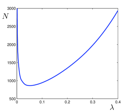
Figure 2: The plasmon number $N$ of the 3D vortex soliton as a function of the nonlinear frequency shift $\lambda$.

The method reduces the corresponding nonlinear problem into a sequence of linear equations (34) which are solved by the conjugate gradient method Dongarra1994 . The Newton-Kantorovich method has a quadratic rate of convergence and typically after several iterations we are able to find the vortex soliton solutions with a very high accuracy (up to a machine one). An example of the vortex soliton solution with $\lambda=0.2$ is presented in Fig. 1.

Figure 3: Self-cleaning of a randomly perturbed stable vortex soliton with $m=1$ after the application of a random perturbation with the parameter $\nu=0.08$. Panels (a), (b) and (c) display the shape of the perturbed vortex at the initial moment, $t=0$, at $t=6$ and at $t=200$. The unperturbed vortex has $\lambda=0.2$ and $N=1347$.

The plasmon number (10) of the vortex soliton given by the expression

$$N=\int|\hat{\mathbf{L}}A|^{2}d\mathbf{r}$$ (29)

is plotted, as a function of the nonlinear frequency shift $\lambda$, in Fig. 2. The minimum of the function, $N_{cr}=863$, is located at $\lambda_{cr}=0.053$.

The physical relevance of any stationary solution depends on whether it is stable. A well known approach to predicting the stability for soliton families in NLSE of any dimension is based on the Vakhitov-Kolokolov (VK) criterion Petviashvili92 ; Vakhitov73 . The VK criterion states that a stationary solution $\sim\exp(i\lambda t)$ with the energy $N$ may be stable if $\partial N/\partial\lambda>0$, and is definitely unstable otherwise. For the fundamental solitons (i. e. ground states), this condition is both a necessary and sufficient one. This criterion, however, does not apply to the equation (7) and moreover, provides a necessary, but generally, not sufficient condition for the stability of vortex solitons. In the region where the VK criterion holds, but the vortices in NLSE are unstable, they are vulnerable to the splitting instability induced by perturbations breaking the azimuthal symmetry Malomed19 .

To investigate the vortex soliton stability within the framework of Eq. (7) we solved numerically the dynamical equations (19) and (20) initialized with our computed vortex solutions with added initial perturbation. The initial condition was taken in the form $E(\mathbf{r},0)=A_{0}(\mathbf{r})[1+\nu f(\mathbf{r})]$, where $A_{0}(\mathbf{r})$ is the numerically calculated solution and $f(\mathbf{r})$ is some function corresponding the perturbation at the initial time $t=0$. We considered two forms of the function $f(\mathbf{r})$. In the first case, $f(\mathbf{r})$ is the white Gaussian noise with the zero mean and variance $\sigma^{2}=1$. In the second case, $f(\mathbf{r})=\sin x+i\cos y$. The parameter of perturbation is $\nu=0.005-0.1$. In both cases perturbations break the azimuthal symmetry. A numerical simulation shows that the vortex soliton turns out to be stable if $\lambda>\lambda_{cr}$ that is in the region formally predicted by VK criterion. We could not see any evidence of the splitting instability at least up to times $t=400$ that is much larger than the characteristic nonlinear time $\sim 1/\lambda$. An example of stable evolution of the vortex soliton with $\lambda=0.2$ is shown in Fig. 3. The initial state of the vortex soliton is perturbed by a rather strong noise with $\nu=0.08$. The vortex soliton cleans up itself from the noise at the characteristic nonlinear time $\sim 1/\lambda$ and then survives over long time.

Though we did not perform the linear stability analysis with the corresponding eigenvalue problem, it seems that the complex eigenvalues (if any) accounting for the splitting instability are sufficiently small. In this connection it is interesting to compare some results concerning the stability of the vortex-soliton solutions obtained for the generalized two-dimensional NLSE of the form

$$i\frac{\partial\psi}{\partial t}+\Delta_{\bot}\psi+f(|\psi|^{2})\psi=0,$$ (30)

where $f(|\psi|^{2})$ is an arbitrary function of the intensity and $\Delta_{\bot}=\partial^{2}/\partial x^{2}+\partial^{2}/\partial y^{2}$. Following the approach originally proposed in Refs. Soto-Crespo92 ; Soto-Crespo94 , an approximate analytical estimate for the growth rate of azimuthal instability against the azimuthal perturbations $\sim\exp(i\Omega t+iM\theta)$ of the vortex soliton in the model (30) can be written as Berge2006

$$\mathrm{Im}\,\Omega=\frac{M}{\bar{r}_{m,\lambda}}\mathrm{Re}\left[2f^{{}^{\prime}}(|\psi_{0}|^{2})|\psi_{0}|^{2}-\frac{M}{\bar{r}_{m,\lambda}^{2}}\right]^{1/2}$$ (31)

Here the prime stands for the derivative, $\bar{r}_{m,\lambda}$ is the mean value of the vortex radius defined in Ref. Soto-Crespo92 and the amplitude $|\psi_{0}|\equiv|\psi_{m,\lambda}|$ is evaluated at $r=\bar{r}_{m,\lambda}$ ($m$ is the topological charge and $\lambda$ is the nonlinear frequency shift). For the competing nonlinearity $f(I)=I-I^{2}$ in Eq. (30), where $I=|\psi|^{2}$, the function $f^{{}^{\prime}}(I)$ may be negative so that $\mathrm{Im}\,\Omega=0$ and the vortex turns out to be stable for sufficiently large amplitudes Pego2002 . For the saturating nonlinearity with $f(I)=I/(1+I)$ the function $f^{{}^{\prime}}(I)$ is always positive and spinning solitons are unstable in agreement with the rigorous analysis Skryabin1998 . In the case of the exponential saturating nonlinearity $f(I)=1-\exp(-I)$, which has not been previously studied, the first term in the square brackets in Eq. (31), though positive, is exponentially small for large amplitudes and the instability is either practically suppressed or absent. In our case, by analogy with the model (30) one could also expect strong decreasing of the growth rate or full stability of the vortex soliton.

It is important to emphasize that at the critical value $\lambda_{cr}$ the vortex soliton characteristic size $\sim\lambda_{cr}^{-1/2}$ is much larger than the electron Debye length so that the Landau damping is negligible. The Landau damping is still small enough for the solitons with $\lambda\lesssim 0.2$, however for larger $\lambda$ values one has to take into account the damping.

While the fundamental soliton corresponds to the ground state of the nonlinear eigenvalue problem, the vortex soliton may be regarded as an excited state. Under certain conditions, one can expect emergence of the excited states (sometimes with a sufficiently long lifetime) just as in linear problems. For example, dynamical generation of the vortex soliton clusters from the initial condition in the form of the fundamental soliton with superimposed discontinuous phases was demonstrated in the two-dimensional NLSE with the parabolic trapping potential Lashkin2012 .

IV Conclusion

In conclusion, we have shown the possibility of existence in an unmagnetized plasma of the stable 3D solitons with the nonzero angular momentum (vortex solitons). Such coherent structures, as well as fundamental solitons, may be considered as ”elementary bricks” of strong Langmuir turbulence. The real picture of strong Langmuir turbulence – collapsing cavitons or quasistationary structures interacting with quasilinear waves – is apparently largely dependent on excitation conditions, amplitudes and spatial scales of initial perturbations.

*

Appendix A Petviashvili and Newton-Kantorovich iteration schemes

The Petviashvili iteration procedure Petviashvili76 ; Lakoba07 for Eq. (28) at the $n$-th iteration is

$$A_{\mathbf{k}}^{(n+1)}=sG_{\mathbf{k}}^{-1}B_{\mathbf{k}}^{(n)},$$ (32)

where $s$ is the so called stabilizing factor defined by

$$s=\left(\frac{\int|A_{\mathbf{k}}^{(n)}|^{2}d\mathbf{k}}{\int A_{\mathbf{k}}^{\ast,(n)}G_{\mathbf{k}}^{-1}B_{\mathbf{k}}^{(n)}d\mathbf{k}}\right)^{\alpha}.$$ (33)

and $\alpha>1$. For the power nonlinearity, the fastest convergence is achieved for $\alpha=p/(p-1)$, where $p$ is the power of nonlinearity Lakoba07 . For the exponential nonlinearity in (23) we use, depending on $\lambda$, empirical value $\alpha=1.2-1.3$.

The equation (22) is rewritten in the form $F(\mathbf{A})=0$ with $\mathbf{A}=(A,A^{\ast})$). Then Newton-Kantorovich iteration scheme Kantorovich39 ; Kantorovich73 is

$$F^{{}^{\prime}}(\mathbf{A}^{(n)})\mathbf{A}^{(n+1)}=F^{{}^{\prime}}(\mathbf{A}^{(n)})\mathbf{A}^{(n)}-F(\mathbf{A}^{(n)}),$$ (34)

where the prime stands for the Frechet derivative of the operator $F(\mathbf{A})$ at the point $\mathbf{A}_{0}$ defined as

$$F^{{}^{\prime}}(\mathbf{A}_{0})\mathbf{A}=\lim_{h\rightarrow 0}[F(\mathbf{A}_{0}+h\mathbf{A})-F(\mathbf{A}_{0}))].$$ (35)

Calculating the Frechet derivative reduces to linearizing the corresponding nonlinear operator in $h$ and $F^{{}^{\prime}}(\mathbf{A}^{(n)})$ is determined by

$$F^{{}^{\prime}}(\mathbf{A}^{(n)})h=-\lambda h+\Delta h+\hat{\mathbf{L}}\cdot(\alpha\hat{\mathbf{L}}h-\beta\hat{\mathbf{L}}h^{\ast}),$$ (36)

where

$$\alpha=[\exp(-|\hat{\mathbf{L}}A^{(n)}|^{2})-1]-\exp(-|\hat{\mathbf{L}}A^{(n)}|^{2})|\hat{\mathbf{L}}A^{(n)}|^{2}$$ (37)

and

$$\beta=\exp(-|\hat{\mathbf{L}}A^{(n)}|^{2})(\hat{\mathbf{L}}A^{(n)})^{2}.$$ (38)

References

- (1) B. A. Malomed, Physica D 399, 108 (2019).
- (2) Yu. S. Kivshar and G. P. Agrawal , Optical Solitons: From Fibers to Photonic Crystals (Academic, San Diego, 2003).
- (3) V. I. Berezhiani, S. M. Mahajan, Z. Yoshida, and M. Pekker, Phys. Rev. E 65, 046415 (2002).
- (4) V. I. Berezhiani, S. M. Mahajan and N. L. Shatashvili, J. Plasma. Physics 76, 467 (2010).
- (5) A. I. Yakimenko, Y. A. Zaliznyak, and Y. Kivshar, Phys. Rev. E 71, 065603(R) (2005).
- (6) V. M. Lashkin, Phys. Plasmas 14,102311 (2007).
- (7) V. I. Petviashvili and O. A. Pokhotelov, Solitary Waves in Plasmas and in the Atmosphere (Gordon and Breach, Reading, PA, 1992).
- (8) W. Horton and Y.-H. Ichikawa, Chaos and Structures in Nonlinear Plasmas (World Scientific, Singapore, 1996).
- (9) V. M. Lashkin, Phys. Rev E 96, 032211 (2017).
- (10) E. A. Kuznetsov, A. M. Rubenchik, V. E. Zakharov, Phys. Rep. 142, 103 (1986).
- (11) A. Ruocco, G. Duchateau1, V. T. Tikhonchuk, S. Hüller, Plasma Phys. Control. Fusion 61, 115009 (2019).
- (12) V. I. Petviashvili, Sov. J. Plasma Phys. 2, 257 (1976).
- (13) T. I. Lakoba, J. Yang, J. Comput. Phys. 226, 1668 (2007).
- (14) L. V. Kantorovich, Acta Mathematica 71 63 (1939).
- (15) A. M. Ostrowski, Solution of Equations in Euclidean and Banach Spaces (Academic Press, New York, 1973).
- (16) V. E. Zakharov, Sov. Phys. JETP 35, 908 (1972).
- (17) S. V. Antipov, M. V. Nezlin, A. S. Trubnikov, I. V. Kurchatov, Physica D 3, 311 (1981).
- (18) A. Y. Wong, P. Y. Cheung, Phys. Rev. Lett. 52, 1222 (1984).
- (19) P. Y. Cheung, A. Y. Wong, Phys. Fluids 28, 1538 (1985).
- (20) E. A. Kuznetsov, Sov. J. Plasma Phys. 2, 178 (1976).
- (21) M. M. Ŝkoriĉ, D. ter Haar, Physica 98C , 211 (1980).
- (22) T. A. Davydova, A. I. Yakimenko, Yu. A. Zaliznyak, Phys. Lett. A 336 , 46 (2005).
- (23) E. W. Laedke and K. H. Spatschek, Phys. Rev. Lett. 52, 279 (1984).
- (24) P. K. Kaw, G. Schmidt, and T. Wilcox, Phys. Fluids 16, 1522 (1973).
- (25) N. G. Vakhitov, A. A. Kolokolov, Radiophys. Quantum Electron. 16 783 (1973).
- (26) J. M. Soto-Crespo, E. M. Wright, N. N. Akhmediev, Phys. Rev A 45, 3168 (1992).
- (27) J. Atai, Y. Chen, J. M. Soto-Crespo, Phys. Rev A 49, R3170 (1994).
- (28) A. Vincotte, L. Bergé, Physica D 223, 123 (2006).
- (29) R. L. Pego and H. A. Warchall, J. Nonlinear Sci. 12, 347 (2002).
- (30) D. V. Skryabin and W. J. Firth, Phys. Rev. E 58, 3916 (1998).
- (31) V. M. Lashkin, A. S. Desyatnikov, E. A. Ostrovskaya, and Y. S. Kivshar, Phys. Rev A 85, 013620 (2012).
- (32) R. Barret, M. Berry, T. F. Chan, J. Demmel, J. M. Donato, J. Dongarra, V. Eijihout, R. Pozo, C. Romine, H. Van der Vorst, Templates for the Solution of Linear Systems: Building Blocks for Iterative Methods (SIAM, Philadelphia, 1994).