Branching ratio of the super-allowed $\beta$ decay of ¹⁰C

Abstract

In an experiment performed at the ISOLDE facility of CERN, the super-allowed $\beta$-decay branching ratio of ¹⁰C was determined with a high-precision single-crystal germanium detector. In order to evaluate the contribution of the pile-up of two 511 keV $\gamma$ quanta to one of the $\gamma$-ray peaks of interest at 1021.7 keV, data were not only taken with ¹⁰C, but also with a ¹⁹Ne beam. The final result for the super-allowed decay branch is 1.4638(50)%, in agreement with the average from literature.

1 Introduction

Super-allowed 0${}^{+}\rightarrow$ 0${}^{+}\beta$ decay is a powerful tool to explore properties of the fundamental weak interaction. These transitions have been used to test the conserved vector current (CVC) hypothesis as well as to determine the vector coupling constant $G_{v}$ and the V_ud Cabbibo-Kobayashi-Maskawa quark mixing matrix element hardy15 . To achieve these goals, the $ft$ value of 0${}^{+}\rightarrow$ 0⁺ $\beta$ decays has to be measured precisely, which requires precise knowledge of the $\beta$-decay Q value, half-life and super-allowed branching ratio for as many nuclei as possible. Once this is achieved, the corrected $\mathcal{F}$t values can be determined:

$$Ft=ft(1+\delta_{R}^{\prime})(1+\delta_{NS}-\delta_{C})=\frac{k}{2G_{v}^{2}(1+\Delta_{R}^{v})}$$

where $\delta_{R}^{\prime},\delta_{NS}$, and $\Delta_{R}^{v}$ are radiative corrections and $\delta_{C}$ is an isospin breaking corrections. With these corrected $\mathcal{F}$t values, physics beyond the standard model (SM) of particle physics can be explored.

These extensions of the SM can be of different nature, one of them being the addition of scalar or tensor currents to the well-known vector and axial-vector currents. The possible addition of a small scalar contribution to the Fermi transitions can be tested with 0${}^{+}\rightarrow$ 0${}^{+}\beta$ decay. With only the vector current contributing, the corrected $\mathcal{F}$t values should be constant, whereas the addition of a scalar term yields $\mathcal{F}$t values which, due to an additional term in the Fermi function, are dependent on the Q value of the decay. This can be observed in particular for nuclei with small Q values, i.e., in the series of well-known 0${}^{+}\rightarrow$ 0${}^{+}\beta$ decays, for the lightest super-allowed emitters ¹⁰C and ¹⁴O (see Figure 7 in  hardy15 ).

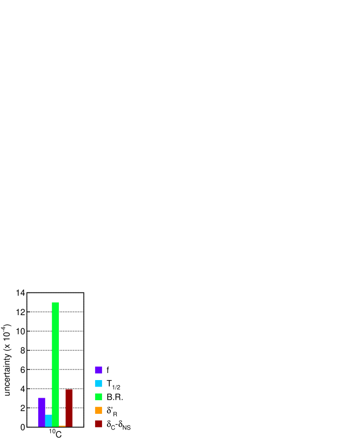
Figure 1: Error budget for the $\mathcal{F}$t value of ¹⁰C. By far the highest contribution comes from the super-allowed branching ratio of ¹⁰C.

Table 1: Literature values for the super-allowed branching ratio of ¹⁰C prior to the present experiment.

Sherr	Freeman	Robinson	Kroupa	Nagai	Fujikawa	Savard	average
et al. sherr53	et al. freeman69	et al. robinson72	et al. kroupa91	et al. nagai91	et al. fujikawa99	et al. savard95	hardy15
1.65(20) %	1.523(30) %	1.465(14) %	1.465(9) %	1.473(7) %	1.4625(25) %	1.4665(38) %	1.4646(19) %

Before the present work, the world data for ¹⁰C decay were as follows hardy15 :

• the Q value is Q_EC = 1907.994(67) MeV yielding a statistical rate function of f = 2.30169(70)

• the half-life is T_1/2 = 19301.5(25) ms dunlop16

• the super-allowed branching ratio is BR = 1.4646(19) %. This value stems effectively from two experiments performed with large germanium detector arrays. Values of 1.4665(38)% fujikawa99 and 1.4625(25)% savard95 were obtained. Table 1 gives all literature values.

• the theoretical corrections are $\delta_{R}^{\prime}$ = 1.679(4)% and $\delta_{C}-\delta_{NS}$ = 0.520(39)%.

The value of $\Delta_{R}^{v}$ is presently discussed in several theoretical papers seng18 ; czarnecki19 ; gorchtein19 ; seng19 ; seng20 and has a considerable uncertainty. However, as it is not affecting the determination of the corrected $\mathcal{F}$t value for ¹⁰C, we refrain from commenting on its value.

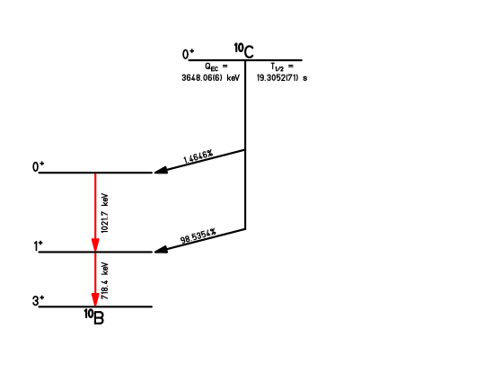
Figure 2: Partial decay scheme of ¹⁰C. The quantities measured in the present experiment are given in red.

In Figure 1, we plot the uncertainties of these different inputs for the determination of the $\mathcal{F}$t value of ¹⁰C. The branching ratio is by far the most important contributor to the error bar of the $\mathcal{F}$t value for this nucleus. The aim of the present work is to contribute to the improvement of the super-allowed branching ratio of ¹⁰C. Although the decay scheme of this nucleus is quite simple (see Figure 2), the difficulty in the present endeavour arises from the fact that the $\gamma$ ray at 1021.7 keV has to be measured in the presence of possible pile-up of two 511 keV photons in the $\gamma$-ray detector. Therefore, in addition to the measurement of the ¹⁰C decay itself, additional measurements with ¹⁹Ne have been performed, a nucleus which is also a $\beta^{+}$ emitter with a half-life (17.22 s) and a $Q$ value (3238.4 keV) similar to those of ¹⁰C but no $\gamma$ ray close to the pile-up energy.

2 Experimental set-up

The experiment was conducted at the ISOLDE facility of CERN. A 1.4 GeV proton beam from the PS-Booster impinged on a CaO target with an maximum intensity of about 2$\mu$A for the production of ¹⁰C and about a factor of 5 less for the production of ¹⁹Ne. ¹⁰C and ¹⁹Ne were ionised with a VD7 plasma ion source penescu10 . After mass selection with the ISOLDE high-resolution separator HRS, the beam was sent to the LA1 experimental station, where the detector set-up was mounted. The ISOLDE beam gate was constantly open to accept the full intensity extracted from the ISOLDE target. However, the number of proton pulses in a CERN ”supercycle” was varied over the whole experiment ranging from 3 out of about 30 cycles per supercycle to half of the cycles in a supercycle. For runs where we took half of the cycles in a supercycle (in fact one out of two cycles), the detection rate was constant over the course of the run. For runs with only a few cycles per supercyle, they were spread roughly regularly over the supercycle (e.g. cycles 1, 11, and 21 for 30 cycles per supercycle) to have a detection rate as constant as possible in our detectors.

There was no detectable contamination for the ¹⁹Ne beam, whereas the situation was worse for the ¹⁰C runs. At the beginning of the experiment, tests were made by the target team to check whether the production of atomic ¹⁰C is more favourable than the production of ¹⁰C¹⁶O molecules. It turned out that CO molecules are produced with an intensity about a factor 2 larger than atomic ¹⁰C. In addition, the HRS could not be set on masses as small as A=10. However, at mass 26, not only ¹⁰C¹⁶O arrived at the detection station, but also ¹²C¹⁴O and ¹³N₂. The production of ¹²C¹⁴O was negligibly small (2.8$\times$10^-4 compared to ¹⁰C¹⁶O). ¹³N₂ was produced as much as ¹⁰C¹⁶O and gave thus twice as much 511 keV $\gamma$ rays.

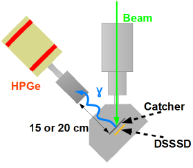
Figure 3: The experimental set-up of the present experiment. In the vacuum chamber, a catcher foil intercepted the ¹⁰C¹⁶O and ¹⁹Ne beams. The implantation distribution was followed on-line by detecting the $\beta$ particles in a double-sided silicon strip detector installed about 1 mm behind the catcher foil. The precisely calibrated germanium detector was installed at a distance of 15.00(1) cm or 20.00(1) cm from the catcher foil.

The detection set-up (Figure 3) consisted of a vacuum chamber with an aluminium catcher foil (200$\mu$m thickness) and a double-sided silicon strip detector (DSSSD, 500$\mu$m thickness) with 16 X and 16 Y strips and a pitch of 3mm, installed about 1 mm behind the catcher foil. The DSSSD served to optimise and control the implantation profile of the beam on the catcher foil. Gamma rays were detected outside the vacuum chamber (1.9 mm window of aluminium) by a precisely efficiency calibrated germanium detector blank14ge at a distance of 15 or 20 cm. The full-energy detection efficiency for the $\gamma$ rays of interest at 718.3 keV and 1021.7 keV were 0.28279(17)% and 0.22348(15)% at a distance of 15 cm as well as 0.17671(66)% and 0.14157(83)% at 20 cm.

The germanium detector was precisely calibrated in efficiency at a distance of 15 cm blank14ge . If the detector model we use in the simulations were perfect, the efficiencies calculated at a distance of 20 cm should be correct, too. However, an inspection of the measurements at 15 cm and at 20 cm (see below) evidenced a systematically higher branching ratio at 20 cm. We therefore embarked in a new series of calibration measurements of the germanium detector efficiency at 20 cm. For this purpose, we performed measurements at 15 cm and 20 cm with sources of ⁶⁰Co, ¹³⁷Cs, and ²⁰⁷Bi. The measurements with the two ⁶⁰Co lines and the 1063 keV line of ²⁰⁷Bi allowed us to determine the efficiency ratio between the 15 cm and 20 cm positions for an energy close to the 1022 keV line of ¹⁰C, whereas we used the ¹³⁷Cs $\gamma$ ray at 662 keV and the ²⁰⁷Bi line at 570 keV to determine the experimental efficiency ratio for the 718 keV $\gamma$ ray for ¹⁰C. We assumed that the variation of the ratios with energy is sufficiently small so that the slightly lower calibration energies for the 718 keV line and the slightly higher calibration lines for the 1022 keV line yield acceptable ratios for the energies of ¹⁰C.

The finding was that the calculated efficiencies of the 718 keV and 1022 keV lines at 20 cm were factors of 0.8(29)$\times$10^-3 and 4.8(15)$\times$10^-3 too small, respectively. We therefore corrected the calculated efficiencies at 20 cm with these factors. For the uncertainties, we added in quadrature the error bar of the correction factor and the correction factor itself to the uncertainty of the calculated efficiency, which yields in the end the larger error bars for the efficiencies at 20 cm.

Two data acquisitions (DAQ) were run in parallel. The first DAQ had a single parameter which was the germanium energy. In addition, a scaler module was read for each event. This scaler counted the number of proton pulse sent to ISOLDE since the beginning of the run, the number of $\gamma$-ray triggers from the germanium detector and the time of each event with a precision of 1 millisecond. This data acquisition was triggered only by the germanium detector.

The second data acquisition was only used on-line. It registered the germanium energy signal and the energy signals from the 32 strips of the DSSSD. Similar to the first DAQ, a scaler registered the proton pulses, the germanium triggers and the time. This DAQ allowed us to optimise the beam implantation profile by detecting the $\beta$-decay position profile with the DSSSD and to supervise it during the experiment. It was triggered by the detection of a $\beta$ particle in the DSSSD. After optimisation, the beam spot was centred on the catcher foil and had a size of about 8 mm (FWHM) in X and Y, negligible compared to the distance of the source from the detector.

3 Data taking

As mentioned in the introduction, the main difficulty in the present experiment is to correctly evaluate the 511 keV - 511 keV pile-up which adds to the 1021.7 keV peak from the decay of ¹⁰C. For this purpose, the ¹⁰C activity transported to the detection set-up was largely varied by taking more or less proton pulses per supercycle which modifies the pile-up probability as a function of the 511 keV detection rate per second squared. In addition, we modified once during the experiment the distance between the radioactive sample and the germanium detector entrance window from 15 cm to 20 cm therefore varying both the total rate and the pile-up probability. This pile-up probability is also directly proportional to the shaping time of the germanium signal. We therefore used two shaping times for the germanium signal of 2$\mu$s and 1$\mu$s. Table 2 gives details about the settings used in the different runs of the experiment.

The idea of these changes in decay rate in the set-up, in distance and in shaping time is that in the end we have to get the same branching ratio, independent of the settings. This procedure is meant to search for systematic errors in our measurements and will be tested below.

Table 2: Settings used throughout the experiment. Germanium signal shaping times and germanium distance were modified several times during the experiment.

isotope	run number	shaping time	distance
10C	42 - 55	2 $\mu$s	15 cm
10C	56 - 97	1 $\mu$s	15 cm
10C	98 - 116	2 $\mu$s	15 cm
19Ne	118 - 127	2 $\mu$s	15 cm
19Ne	128 - 133	1 $\mu$s	15 cm
19Ne	134 - 144	2 $\mu$s	20 cm
10C	145 - 173	2 $\mu$s	20 cm

However, these changes were not enough to quantitatively evaluate the pile-up probability. For this purpose, we spent an important part of the beam time on measurements with ¹⁹Ne (about 18 h as compared to 78 h for ¹⁰C). ¹⁹Ne has decay characteristics similar to ¹⁰C, however, without having a $\gamma$ ray at 1022 keV. Therefore, counts above background in this region can only come from pile-up of two 511 keV $\gamma$ rays. By measuring the 511 keV and the 1022 keV rate, we are able to determine the pile-up probability on an absolute scale.

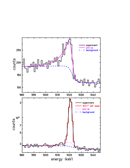
Figure 4: Gamma-ray spectrum in the region of the 1022 keV peak. The upper part shows a spectrum from a ¹⁹Ne run, where the pile-up contribution from two 511 keV $\gamma$ quanta and the background is visible. The lower spectrum contains in addition $\gamma$ rays at 1021.7 keV from the decay of the second excited state of ¹⁰C. The different curves give the different contributions to the spectrum. The pile-up contribution in the lower figure is calculated and subtracted before determining the integral of the peak.

Figure 4 shows the region around E_γ = 1022 keV for a run with a ¹⁹Ne beam and with a ¹⁰C beam. In the ¹⁹Ne case, the spectrum can be described by a background-contribution step function and a Gaussian with a low-energy tail. In the case of ¹⁰C, the additional peak at 1021.7 keV is seen on top of these two contributions.

The pile-up correction as introduced below depends sensitively on the counting rate of the 511 keV $\gamma$ rays. Therefore, a run selection was performed where only runs with a constant 511 keV $\gamma$-ray rate were kept. Changes in this rate were caused by modifications of the CERN supercycle or other problems with the PS-Booster or the ISOLDE front-end during a run. These problems forced us to remove 33 runs out of 99 for the ¹⁰C measurements and 1 run (out of 26) for the ¹⁹Ne measurements totalling about 34% and 3.5% of the running time for each isotope, respectively.

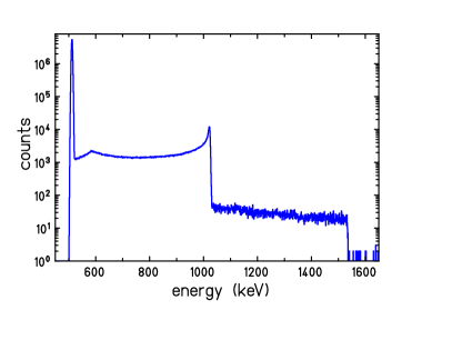
Figure 5: Simulated $\gamma$-ray spectrum for a single-energy $\gamma$ ray of 511 keV. The time distribution of the events was taken from a ¹⁸Ne run (run 118, see figure 7 for the time structure of this run). Depending on the time difference between two events, a total signal energy between 1022 keV (no or negligible time difference between two events) and 511 keV (time difference longer than the signal width) is found. Events above 1022 keV come from triple and quadruple coincidences. The edge at about 600 keV is due to the fact that we use a DAQ time window of 10$\mu$s. For a signal shaping time of 2$\mu$s, the second event starts to be cut by this time constraint.

In order to correctly determine the number of counts under the 1021.7 keV peak, we have to subtract this pile-up contribution. As mentioned earlier, the pile-up of two 511 keV $\gamma$ ray depends quadratically on the rate of these $\gamma$ rays and on the time difference between the two events. If the time difference is close to zero, an energy signal at 1022 keV results. The more the two $\gamma$ rays are separated in time, the lower is the signal energy with the lower limit being a 511 keV signal. This limit corresponds in fact to the case where there is no pile-up of the signals in the detector. The exact shape of the pile-up peak in the spectrum depends on the signal shape from the electronics (in particular the shaping amplifier).

Figure 5 shows a simulation where only 511 keV $\gamma$ rays were considered. The events between 511 keV and 1022 keV come from two events which overlap more and more in time. At 1022 keV, a perfect overlap is reached. Above 1022 keV, triple coincidences and above 1533 keV quadruple coincidences come into play. The pile-up probability for each run can be determined by these simulations as the number of counts above the 511 keV peak. It varied as a function of the total counting rate of the germanium detector between 0.2% and 2% for the different runs. Details of the MC simulations will be given below.

3.1 ¹⁹Ne runs

We used the ¹⁹Ne runs to determine the pile-up probability. For this purpose, the pile-up peak at 1022 keV and the 511 keV peak were fit to determine their functional form and their intensity. It was found that the shape of the 1022 keV peak is always the same, independent of the signal shaping time or the pile-up rate. Only the pile-up probability, i.e. the number of counts in the pile-up peak, depends on these two parameters. Therefore, the 511 keV rate and the 1022 keV pile-up rate can be linked by the following formula:

$$N_{1022}=N_{511}^{2}*\tau$$ (1)

where N_x are the rates of the 511 keV and 1022 keV peaks and $\tau$ is a pile-up time. We found in addition that $\tau$ is constant for a fixed experimental shaping time of the experiment electronics. To go from a shaping time of 2$\mu$s (most of the runs) to 1$\mu$s, the pile-up time has simply to be divided by two. Figure 6 shows the pile-up times for all ¹⁹Ne runs as determined with the formula above. Although the $\chi^{2}$ of all the average values is about 2, we consider that we can use a constant pile-up time for all runs.

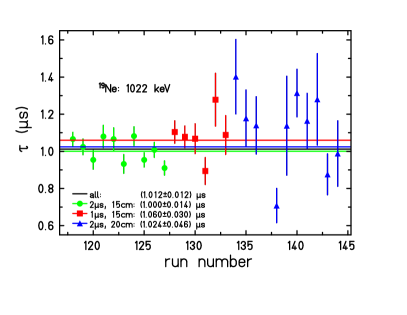
Figure 6: Pile-up times as determined from formula 1 for each ¹⁹Ne run. The average values for the different settings agree with each other satisfactorily, although the $\chi^{2}$ is only about 2 for the different averages. The values for the 1$\mu$s runs were multiplied by a factor 2.

Now that we have determined the exact functional form and the pile-up time with the ¹⁹Ne runs, we can use this information for the pile-up subtraction of the ¹⁰C runs (see Figure 4). However, this procedure is only correct, if the time distribution is the same for both nuclei. An inspection of this time distribution (see Figure 7) shows that this is not at all the case. The noble gas character of ¹⁹Ne allows this isotope to diffuse and effuse in the ISOLDE target - ion-source (TIS) ensemble extremely rapidly. Therefore, a well-pronounced time structure due to the proton impact on the ISOLDE target and the ¹⁹Ne half-life is seen in the case of ¹⁹Ne (lower figure), which is completely absent in the case of the ¹⁰C¹⁶O molecules and its contaminants, which are extracted from the TIS ensemble much slower that the proton beam time structure and the ¹⁰C half-life.

As in the case of ¹⁹Ne this time distribution is not constant, a correction factor has to be applied when comparing ¹⁹Ne and ¹⁰C. This factor will be determined in the following via Monte-Carlo (MC) simulations.

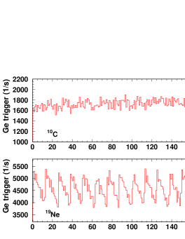
Figure 7: The two figures show the different event time structures as seen by the germanium detector. The upper part shows the germanium triggers as a function of time for a run with the ¹⁰C activity, whereas the lower spectrum shows the same information for a ¹⁹Ne run. Although both nuclei have approximately the same half-life, the time structure at the experiment is largely different due to the different release properties for CO molecules and the associated contaminants and ¹⁹Ne. In the latter spectrum, the impinging of the PS Booster proton beam on the ISOLDE target (every 12s and 13.2s, multiples of the PS Booster time structure of 1.2 s) is clearly visible. For the ¹⁰C runs, the contaminants ¹⁴O and ¹³N with their longer half-lives also contribute to wash out the time structure.

3.2 Monte-Carlo simulations

If the time structure of the ¹⁹Ne and the ¹⁰C runs were the same, the pile-up probability determined with ¹⁹Ne could be used directly for the ¹⁰C runs. However, this is not the case. Therefore, we developed a MC procedure to determine a correction factor to correlate the pile-up probabilities of ¹⁹Ne and ¹⁰C.

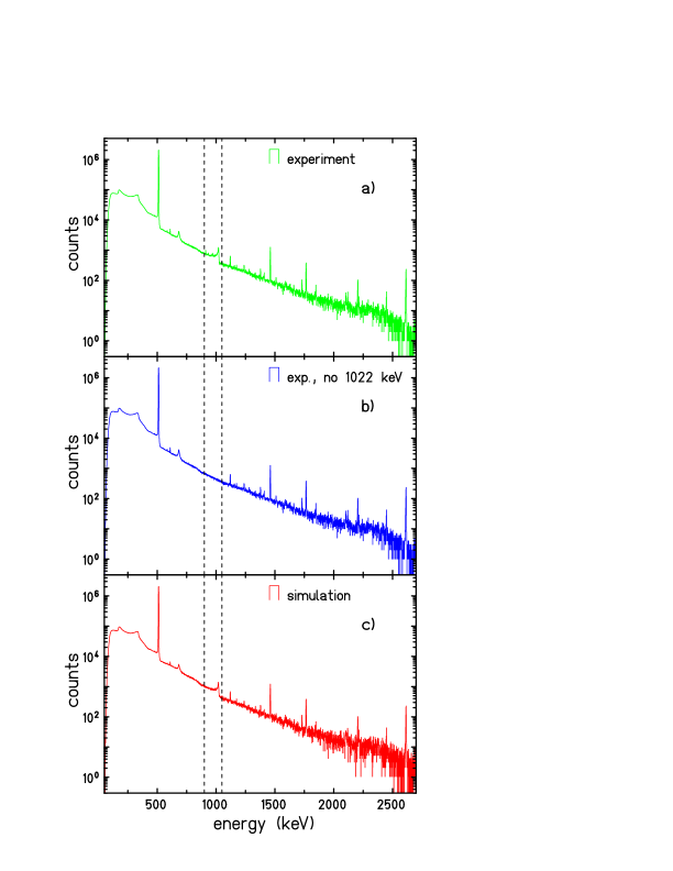
Figure 8: Experimental spectra and a spectrum generated by a Monte-Carlo procedure. a) Experimental spectrum from a ¹⁹Ne run over basically the full energy range. b) Same spectrum, however, with the 1022 keV pile-up peak removed and the 511 keV peak increased to compensate for the removal of counts from this peak by pile-up (see text for details). c) Simulated spectrum from a Monte-Carlo simulation which uses as inputs the energy distribution from the spectrum in b) and the event time structure as displayed in fig. 7. The dashed vertical lines indicate the region where the effect of pile-up of two 511 keV $\gamma$ rays was removed.

This MC procedure uses the energy spectrum of each individual run and the associated time structure we measured with the scaler module with a precision of 1 ms. Within one millisecond, we distributed the events randomly. In order to simulate the pile-up, we first removed from the experimental spectrum (see Figure 8a) all counts above background in the region of the 1022 keV peak. For this purpose, we first set all channels between 900 keV and 1050 keV to zero and added then a smooth background with statistical fluctuations. In addition, we increased the number of counts in the 511 keV peak by the pile-up probability (0.2% - 2% for the different runs, see figure 5, which allowed us to determine the percentage of 511 keV events removed from the 511 keV peak due to pile-up) to produce a 511 keV peak ”without the effect of pile-up losses in this peak”. The result is shown in Figure 8b. This is then the energy input for the MC simulations. When used together with the event time distribution we can generate a simulated spectrum with its pile-up contribution (Figure 8c).

The only free parameter in these simulations is the ”simulation shaping time”, a parameter in the functional form of the germanium detector signal used in the simulations which is equivalent to the experimental shaping time and varies the time width of the signal. It was adjusted such that it matched the time structure of the experimental signal.

This procedure can be applied to the ¹⁹Ne runs but also to the ¹⁰C runs, where in addition to the pile-up counts also the 1021.7 keV counts are removed. As we can not remove all pile-up events from the input energy spectrum (we correct only the 511 keV and the 1022 keV regions), the simulated spectrum differs from the experimental one by several aspects. For example, the simulated spectrum is generally shifted towards higher energies, because the experimental input spectrum contains $\gamma$ rays that are already piled-up. The simulation further piles-up these same events and shifts events to higher energies. This is particularly visible below 511 keV where counts in the spectrum are lost. However, as we are only interested in the regions around the 511 keV and the 1022 keV peaks, we believe that this procedure is sufficiently correct.

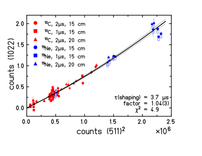
Figure 9: Results from the MC simulations of all runs (see text for details). The number of counts in the 1022 keV pile-up peak is plotted versus the number of counts in the 511 keV peak squared. This plot allows us to readjust the data from the ¹⁹Ne runs by a small factor to take into account the different event time structures of the ¹⁰C and the ¹⁹Ne runs. The ¹⁹Ne data have to be increased by a factor of 1.04(3). The line is the fit of the data after correction with its uncertainty (dashed lines). The open blue symbols are equivalent to the full blue symbols before multiplying them with the scale factor.

Once these simulations were completed, the 511 keV and the 1022 keV peaks were fit as for the experimental spectra. The integrals of these peaks are plotted in Figure 9. In order to determine the matching factor between the ¹⁹Ne and the ¹⁰C data, we fit these data with a second-order polynomial with a free scaling factor for the ¹⁹Ne data to account for the different time structure. The result is a scale factor of 1.04(3). The error bar was determined by varying the simulation shaping factor by $\pm$ 200 ns which is roughly the parameter range where the experimental and the simulation signal shape are in good agreement.

3.3 Pile-up test with the 718 keV $\gamma$ ray of ¹⁰C

A direct test of the pile-up correction during the ¹⁰C runs is not possible with the 511 keV - 511 keV pile-up, because on top of the pile-up peak, the $\gamma$ rays of energy 1021.7 keV add. However, the pile-up can at least be checked to some extent with the pile-up of two $\gamma$ rays of 718 keV. For these $\gamma$ rays, the statistics is about a factor of 10 lower than for 511 keV $\gamma$ rays, but it allows us nonetheless to test the correction.

The same analysis as for the 511 keV pile-up has therefore been done also for this $\gamma$ ray. By means of equation 1 we determined the pile-up time $\tau$ run by run. The result is shown in Figure 10. The pile-up time is in perfect agreement with the value obtained with the 511 keV pile-up during the ¹⁹Ne runs and of the order of 1 $\mu$s (to be compared to Figure 6).

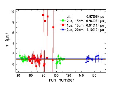
Figure 10: Pile-up times as determined for all ¹⁰C runs from the pile-up of two 718 keV $\gamma$ rays from the decay of the first excited state of ¹⁰C. The runs from 78 to 98 are very low statistics runs and thus have large fluctuations. The values for the 1$\mu$s runs were multiplied by a factor of 2.

4 Results

4.1 Results with standard analysis parameters

The results for the super-allowed branching ratio of ¹⁰C are obtained run by run as follows. For each ¹⁰C run, three peaks are fitted: (i) the 511 keV annihilation peak, (ii) the 718 keV peak from the $\gamma$ decay of the first excited state of ¹⁰B to its ground state, and (iii) the 1021.7 keV peak from the decay of the second excited state of ¹⁰B to its first excited state after subtraction of the pile-up contribution. The pile-up contribution is obtained from the counting rate of the 511 keV $\gamma$ rays by means of equation 1 and an additional small correction factor to take into account the difference in time structure between a ¹⁹Ne and a ¹⁰C run (see section 3.2). The number of pile-up counts thus determined is subtracted from the $\gamma$-ray spectrum with the correct pile-up peak shape after which the 1021.7 keV peak can be fitted with a Gaussian and a background function.

As there is no $\beta$-decay feeding of the ground state of ¹⁰B within the limits of the precision of our experiment, the super-allowed branching ratio of interest is obtained from the efficiency-corrected counting-rate ratio of 1021.7 keV to 718 keV $\gamma$ rays. Figure 11 shows this branching ratio for the different ¹⁰C runs. Averaging these run-by-run results yields a branching ratio of BR = 1.4638(39)% with a normalised $\chi^{2}_{\nu}$ = 1.18. This result contains already the increase of the uncertainty by the square root of the $\chi^{2}_{\nu}$.

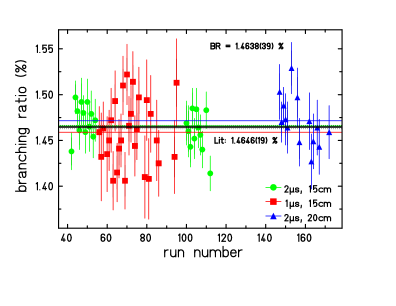
Figure 11: Super-allowed branching ratio as determined run by run. The average of all data is BR = 1.4638(39)% with $\chi^{2}_{\nu}$ = 1.18 (already included in the error bar given). The individual averages are 1.4660(48)% (2$\mu$s, 15 cm), 1.4591(65)% (1$\mu$s, 15 cm), and 1.4717(111)% (2$\mu$s, 20 cm). The $\chi^{2}_{\nu}$ values are 0.99, 1.39, and 1.11 and were used to inflate the uncertainties quoted.

4.2 Search for systematic uncertainties

The measurements with different electronics shaping times and with different distances between the activity and the germanium detector agree with one another. The averaging of all individual runs yields a reduced $\chi^{2}_{\nu}$ of 1.18, which is a sign of good agreement of the branching ratios determined for the different runs. In addition, the branching ratios determined as the averages for the different settings (two different shaping times, one additional position) agree with each other (1.4660(48)% (2$\mu$s, 15 cm), 1.4591(65)% (1$\mu$s, 15 cm), and 1.4717(111)% (2$\mu$s, 20 cm)). Therefore, there is no reason to add a systematic uncertainty from the different experimental settings.

A first systematic uncertainty comes from the factor applied between the ¹⁹Ne and ¹⁰C pile-up correction. As stated above, this factor is 1.04(3). By refitting the 1022 keV peak with factors of 1.01 and 1.07, we obtain branching ratios of BR = 1.4664(40)% and 1.4607(41)%. This enables us to determine a systematic deviation with respect to the central value of $\pm$0.0029%.

An additional systematic uncertainty comes from the shape of the pile-up peak that we determined with the ¹⁹Ne data. It is determined by five parameters: (i) the position of the peak kept fixed once optimised, (ii) the sigma of the Gaussian kept also fixed because strongly correlated with the parameters of the tail function (see next parameters), (iii) the step function for the background defined as a certain percentage of the peak height, (iv) the position of the tail on the low-energy side of the peak, and (v) the pile-up time ($\tau$ = 1.012(12)$\mu$s, see equation 1), which determines the number of pile-up counts from the number of counts from the 511 keV counting rate. However, we do not consider the systematic error due to this last parameter, because this parameter being determined in the fit of the ¹⁹Ne data the error is largely included in the variation of the ¹⁹Ne/¹⁰C correction factor. The systematic errors obtained by varying these parameters within their error bars are shown in table 3. With these systematic errors included, we obtain our final experimental result for the super-allowed branching ratio of ¹⁰C of BR = 1.4638(50)%.

Table 3: Error budget for the present experiment. The statistical uncertainty is summed quadratically with the different systematic uncertainties to yield a total uncertainty of 0.0050%.

error type	uncertainty (%)
experimental statistics	0.0038
efficiency simulation	0.0009
pile-up correction:
19Ne/10C pile-up factor	0.0029
background step function	0.0001
tail position	0.0010
total uncertainty	0.0050

5 Discussion and outlook

Our new value of the super-allowed branching ratio of ¹⁰C is in agreement with the literature average of 1.4646(19) %. The error bar is a factor 1.5 to 2 larger than the most precise literature values fujikawa99 ; savard95 . If we average our value with literature values with an uncertainty less than a factor of 10 larger than the smallest error bar, as prescribed in Ref. hardy15 , we obtain a new average branching ratio of BR = 1.4644(18)%.

Our result slightly modifies the previous world average. As our result is mainly statistics limited, a new experiment with an improved beam production and increased purity could allow to yield a competitive result. As an improvement of the production rate of ¹⁰C seems to be difficult to achieve, a higher statistics experiment will therefore require a longer beam time. However, as the present experiment already lasted 5.5 days, a factor of 2 more beam time is certainly a limit. The measurement at 20 cm contributed little to the final result and should certainly be omitted for a future experiment. It would be probably most reasonable to perform a future measurement only with a shaping time of 1 $\mu$s which allows the highest rate with the smallest pile-up contribution.

The production rate of ¹³N₂ was as strong as the rate of ¹⁰C-¹⁶O. This yields twice as much 511 keV $\gamma$ rays from ¹³N₂ than from ¹⁰C-¹⁶O. The contamination from ¹³N₂ could be removed by the use of e.g. a Multi-reflection Time-of-flight Spectrometer (MR-ToF-MS) or a Penning trap with a resolving power in excess of 10⁵. If the 511 keV rate can thus be divided by a factor of 3, the pile-up would decrease by a factor of 10 and become much less of a problem.

6 Conclusion

We have performed a measurement of the super-allowed $\beta$-decay branching ratio of ¹⁰C. After production and separation by the ISOLDE facility, the ¹⁰C-¹⁶O activity was constantly implanted in a catcher foil in front of our precisely efficiency calibrated germanium detector to measure the $\gamma$ rays emitted in the decay of ¹⁰C.

Our result of BR = 1.4638(50)% is a factor of 1.5 to 2 less precise than the most precise literature values. Nevertheless the present result demonstrates that the problems with the pile-up of two 511 keV $\gamma$ rays can be overcome. In a future experiment, a higher precision can be reached with a longer beam time and a better beam purification scheme. However, it will be very challenging to reach the same precision for the branching ratio as for the half-life and the Q value of ¹⁰C.

References

- (1) J. C. Hardy and I. S. Towner, Phys. Rev. C 91, 025501 (2015).
- (2) R. Sherr and J. B. Gerhart, Phys. Rev. 91, 909 (1953).
- (3) J. M. Freeman, J. G. Jenkin, and G. Murray, Nucl. Phys. A 124, 393 (1969).
- (4) D. C. Robinson, J. M. Freeman, and T. T. Thwaites, Nucl. Phys. A 181, 645 (1972).
- (5) M. A. Kroupa, S. J. Freedman, P. H. Barker, and S. L. Ferguson, Nucl. Instrum. Meth. A310, 649 (1999).
- (6) Y. Nagai et al., Phys. Rev. C 43, R9 (1991).
- (7) B. Fujikawa et al., Phys. Lett. B 449, 6 (1999).
- (8) G. Savard et al., Phys. Rev. Lett. 74, 1521 (1995).
- (9) M. R. Dunlop et al., Phys. Rev. Lett. 116, 172501 (2016).
- (10) C.-Y. Seng, M. Gorchtein, H. H. Patel, and M. J. Ramsey-Musolf, Phys. Rev. Lett. 121, 241804 (2018).
- (11) A. Czarnecki, W. J. Marciano, and A. Sirlin, Phys. Rev. D 100, 073008 (2019).
- (12) M. Gorchtein, Phys. Rev. Lett. 123, 042503 (2019).
- (13) C.-Y. Seng, M. Gorchtein, and M. J. Ramsey-Musolf, Phys. Rev. D 100, 013001 (2019).
- (14) C.-Y. Seng, X. Feng, M. Gorchtein, and L.-C. Jin, arXiv:2003.11264v1 (hep-ph, 25 March 2020).
- (15) L. Penescu, R. Catherall, J. Lettry, and T. Stora, Phys. Sci. Instrum. 81, 02A906 (2010).
- (16) B. Blank et al., Nucl. Instr. Meth. A 776, 34 (2014).