Analytical and numerical treatment of perturbed black holes in horizon-penetrating coordinates

Abstract

The deviations of non-linear perturbations of black holes from the linear case are important in the context of ringdown signals with large signal-to-noise ratio. To facilitate a comparison between the two we derive several results of linear perturbation theory in coordinates which may be adopted in numerical work. Specifically, our results are derived in Kerr-Schild coordinates adjusted by a general height function. In the first part of the paper we address the questions: for an initial configuration of a massless scalar field, what is the amplitude of the excited quasinormal mode (QNM) for any observer outside outside the event horizon, and furthermore what is the resulting tail contribution? This is done by constructing the full Green’s function for the problem with exact solutions of the confluent Heun equation satisfying appropriate boundary conditions. In the second part of the paper, we detail new developments to our pseudospectral numerical relativity code bamps to handle scalar fields. In the linear regime we employ precisely the Kerr-Schild coordinates treated by our previous analysis. In particular, we evolve pure QNM type initial data along with several other types of initial data and report on the presence of overtone modes in the signal.

I Introduction

Black hole perturbation theory RW ; Zerilli ; Vishu ; BertiReview ; Nollert ; Kokkotas1999 ; Konoplya is an important tool to study fundamental problems in black hole physics and astrophysics. With the advent of gravitational wave detectors and direct detection of gravitational waves from compact binaries LIGO1 ; LIGO2 ; LIGO3 ; LIGO4 ; LIGO5 ; LIGO6 , results from perturbation theory have become increasingly useful in modeling waveforms for these compact objects. More specifically, the post-merger part of a binary black hole waveform is dominated by a linear combination of damped sinusoids with frequencies characteristic of the mass and spin of the final black hole after merger. These parameters, called quasinormal mode (QNM) frequencies, have been used for testing general relativity (GR) LIGO7 ; LIGO8 ; Li1 ; Li2 ; Li3 and other alternative theories of gravity. It is convenient to use frequencies derived from the linear theory for these tests. With the increase in detector sensitivity and the advent of space based detectors, black hole spectroscopy is poised to become a vital tool for probing possible deviations from GR in the non-linear regime and testing the validity of the no-hair conjecture Israel ; Israel2 . The use of overtone modes have been successful in testing the no-hair conjecture with present gravitational wave detectors Isi . Stronger tests could be performed with increase in detector sensitivity and the advent of space based detectors like LISA.

Several studies have extended the results of the linear theory to higher orders Pullin1 ; Pullin2 ; Pullin3 ; Pullin4 ; Pullin5 and to full numerical relativity (NR) nonlinear1 ; nonlinear2 ; nonlinear3 ; nonlinear4 . However, to the best of our knowledge, a comprehensive study connecting the results from the linear and the non-linear theory in the presence of ‘large’ perturbations is still absent. Several factors, such as second-order QNMs Hiroyuki and the dependence of tail decay rates on the number of dimensions Bizon2009 , suggest that a full non-linear study may reveal new physics. It is towards fulfilling this gap that we have recently been further developing our pseudospectral numerical relativity (NR) code bamps bamps1 ; bamps2 ; bamps3 ; bamps4 ; bamps5 ; bamps6 ; bamps7 , our aim being to build a complete numerical laboratory for perturbation theory experiments. This challenge requires developing new numerical techniques, notably a more robust way to handle black hole excision, the ability to extract waves at null infinity, and data analysis tools to compare linear and non-linear data.

Motivated by observational and theoretical considerations, we would thus like a systematic, quantitative comparison between linear, higher-order perturbative and fully nonlinear solutions with all of these elements computed in the most compatible manner. To facilitate the desired comparison a natural first wish would be to ascertain the direct, dynamical QNM, and backscattering contributions to the signal emanating from sufficiently small, but otherwise generic initial data in both the linear and non-linear contexts. While searching for an answer to this problem, we found that with few important notable exceptions, such as ansorgrodrigo ; Campanelli_2001 ; PhysRevD.64.084016 , most existing calculations have been performed in either Regge-Wheeler or Schwarzschild coordinates LeaverPRD ; Andersson1995 ; Andersson1997 ; Berti2006 ; CaltechGF ; Zhang ; PhysRevD.84.104002 ; PhysRevD.38.1040 ; Frolov:1998wf and therefore are not ideal for comparison with full NR results, where simulations are generally performed in horizon-penetrating coordinates, which may also be hyperboloidal in nature.

In this paper we therefore restrict our attention to the linear regime and construct a Green’s function in horizon-penetrating Kerr-Schild coordinates, alternatively named in this context Eddington-Finkelstein coordinates, offset by an arbitrary height function. The latter can be used to render the slices hyperboloidal, which will be important for future numerics. Plain Kerr-Schild coordinates are already needed for comparison with bamps. A simplification of the massless Klein-Gordon equation to the confluent Heun equation (CHE) Fiziev1 ; Fiziev2 ; Fiziev3 is hence provided at the beginning of section II. We then give a brief overview of the CHE, its exact solutions and asymptotic solutions at large radii in section II.1. A description of QNM boundary conditions in several coordinate systems along with an overview of the analytic continuation method used to construct them is provided in section II.2. The exact Green’s function for the problem is constructed using these solutions in section II.3. This is then used to compute the quasinormal mode excitation factors (QNEFs) in section II.4. Separate approximations for the tail at low, medium and high frequencies are discussed in section II.5. The contribution from the direct part of the signal is discussed in section II.6.

It has been recently suggested that overtone modes may play an important role in modeling the QNM part of the signal London ; Isi ; Giesler . Our analytic calculations and our Green’s function results are valid for arbitrary initial data in an arbitrary time coordinate related to the Kerr-Schild time by a height function $h(r)$. In the second part of the paper, for simplicity we work in the special case of spherical symmetry and evolve various configurations of a massless scalar field on the Schwarzschild background in Kerr-Schild coordinates. This presupposed spherical symmetry ensures that $l\geq 1$ modes are not excited and QNM ringing is comprised of the principal frequency and overtone frequencies of the $l=0$ mode. After a description of the numerical setup, the scalarfield project and the initial data within bamps in section III.1 and III.2, we perform tests of the tail results and determine the number of terms that are needed in a data analysis model to accurately model the numerical results in section III.3. One goal of the work is to investigate the effect of specialized initial data. This is pursued in section III.4, where we employ a method to evolve a pure QNM solution to obtain an arbitrarily long ringing time near the horizon. This allows us to evolve and detect overtones or a linear superposition of them. We then discuss the possibility of detecting overtone modes from generic initial data and discuss the restricted circumstances under which this is possible. Finally, we devise a strategy to prepare specialized initial data with sine-Gaussians which can be used to obtain long ring-down signals, which improves our ability to detect the first overtone substantially, at least for observers far from the horizon. We also demonstrate that irrespective of the initial data the effect of the branch cut present in the Green’s function construction becomes important during intermediate and late time ringing. We then present a brief comparison between the results of our approximate Green’s function (for the direct part of the signal) and the numerics in section II.6. Finally in section IV, we propose a model for QNM ringing which also incorporates the effect of backscattering, and conclude, discussing the shortcomings of the present approach.

II The wave equation in horizon-penetrating coordinates

The realistic problem of interest is to evolve an arbitrary configuration of a massless scalar field in the Schwarzschild spacetime and study the response of the black hole to it. For sufficiently weak matter content, we can perform our simulations in the Cowling approximation, in which the back-reaction from the scalar field on the metric is considered negligible. This simplified problem, which we henceforth refer to as the ‘linear problem’ is amenable to a Green’s function analysis which reveal several interesting physical phenomena whose analogues are observed in the non-linear problem. Our ultimate strategy will be to take approximations of the individual contributions to the Green’s function in the linear problem and compare them with numerical simulations performed in the non-linear regime to quantify the deviations. This paper deals with the linear problem in horizon-penetrating coordinates compatible with NR.

A scalar field signal, as seen by an observer outside the event horizon, shows three generic features: a part from the direct transmission of the initial data followed by QNM ringing and then a tail which, at late times follows a power law. These features arise from three different contributions to the Green’s function: the high frequency arc, the poles and the branch cut respectively. This is depicted schematically in Fig. 1. While calculating the QNM contribution to the signal, we would like to obtain the dynamic excitation amplitudes Andersson1997 as opposed to assigning constant excitation strengths to each QNM. This sidesteps the ‘timing problem’ which arises in the latter approach. The timing problem essentially requires a choice of a starting time for observation such that computed integrals do not diverge after that time. This turns out to be problematic when the initial data is not sharply localized because in that case the starting time is ill-defined Berti2006 .

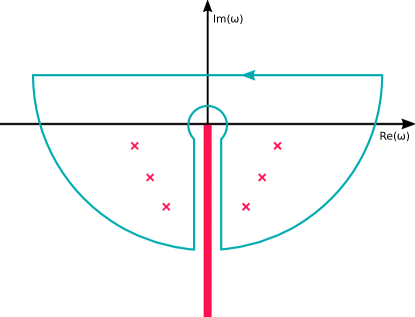
Figure 1: Singularities and branch cut of the Green’s function in the $\omega$ plane. The crosses denote singularities corresponding to the quasinormal mode frequencies while the magenta line indicates the branch cut along the negative imaginary $\omega$-axis. The contour of integration is represented by the blue curve.

The evolution of a massless scalar field is governed by the Klein-Gordon equation,

$$\frac{1}{\sqrt{-g}}\frac{\partial}{\partial x^{\mu}}\left(\sqrt{-g}g^{\mu\nu}\frac{\partial\Phi}{\partial x^{\nu}}\right)=0,$$ (1)

where $g_{\mu\nu}$, $g^{\mu\nu}$ and $g$ are the components of the metric, those of the inverse metric and the determinant of the metric respectively. While our calculations would work also for complex scalar fields, we will evolve real scalar fields presently. We consider two sets of coordinates, the Kerr-Schild coordinates $\{t,r,\theta,\phi\}$ and generalized coordinates $\{T,r,\theta,\phi\}$ with the two time coordinates related by

$$t=T+h(r).$$ (2)

The height function $h$ may be chosen arbitrarily but has a radial asymptotic limit $h\sim r$, $h^{\prime}\sim 1$ near future-null infinity for hyperboloidal slices, spacelike slices which terminate at future null-infinity. In these coordinates, the line element for the Schwarzschild metric can be written as

$$ds^{2} =-\left(1-\frac{2M}{r}\right)dT^{2}+\left(\frac{4M}{r}+\frac{4Mh^{\prime}}{r}-2h^{\prime}\right)dTdr$$

$$+\left(1+\frac{2M}{r}+\frac{4Mh^{\prime}}{r}-h^{\prime 2}+\frac{2Mh^{\prime 2}}{r}\right)dr^{2}$$

$$+r^{2}(d\theta^{2}+\sin^{2}\theta d\phi^{2}).$$ (3)

The field is expanded in a basis of spherical harmonics according to the ansatz,

$$\Phi(T,r,\theta,\phi)=\sum_{l,m}K_{l,m}(T,r)Y_{l,m}(\theta,\phi).$$ (4)

The coefficients $K_{l,m}$ are obtained using

$$K_{l,m}(T,r)=\int_{\theta=0}^{\pi}\int_{\phi=0}^{2\pi}\Phi(T,r,\theta,\phi)Y^{*}_{l,m}(\theta,\phi)\sin\theta d\theta d\phi,$$ (5)

with $*$ denoting the complex conjugate as usual. An initial configuration of the scalar field is provided by specifying $K_{l,m}(0,r)$ and $\left.\partial_{T}K_{l,m}(T,r)\right|_{T=0}$ for every $\left(l,m\right)$. The time evolution of the scalar field can then be computed using the retarded Green’s function

$$K_{l,m}(T,r) =\int G(T,r,r^{\prime})\partial_{T}K_{l,m}(T,r^{\prime})|_{T=0}dr^{\prime}$$

$$+ \quad\int\partial_{T}G(T,r,r^{\prime})K_{l,m}(0,r^{\prime})dr^{\prime}.$$ (6)

Our main objective throughout the rest of the analysis is to compute the different parts of the retarded Green’s function for the QNMs, the tail and the direct transmission of the initial data. To ensure that causality is respected, the above convolution is only performed over the part of the initial data which lies within the past light cone of the observer. To determine this, the coordinate light-speeds of the left moving and right moving solutions must be computed from the roots of the quadratic equation for $v=dr/dT$

$$\quad\left(1+\frac{2M}{r}+\frac{4Mh^{\prime}}{r}-h^{\prime 2}+\frac{2Mh^{\prime 2}}{r}\right)v^{2}$$

$$+\left(\frac{4M}{r}+\frac{4Mh^{\prime}}{r}-2h^{\prime}\right)v-\left(1-\frac{2M}{r}\right)=0.$$ (7)

In Kerr-Schild coordinates, that is with $T=t$, and thus $h=0$, the upper limit of the integration is $r^{\prime}=r+T$ while the lower limit is obtained by solving for $r^{\prime}$ in

$$r^{\prime}+4M\log(r^{\prime}-2M)=r+4M\log(r-2M)-T.$$ (8)

To reduce the wave equation into an ordinary differential equation, we perform a Laplace transformation

$$\hat{G}(\omega,r,r^{\prime})=\int_{0}^{\infty}G(T,r,r^{\prime})e^{i\omega T}dT,$$ (9)

with the inverse transform defined as

$$G(T,r,r^{\prime})=\frac{1}{2\pi}\int_{-\infty+ic}^{\infty+ic}\hat{G}(\omega,r,r^{\prime})e^{-i\omega T}d\omega,$$ (10)

where $c$ is some positive number.

The retarded Green’s function in the frequency domain can then be constructed from two linearly independent solutions to the ordinary differential equation,

$$r(r-2M)\frac{d^{2}\hat{K}_{l,m}}{dr^{2}}+2\big{(}r-M-2i\omega Mr$$

$$+i\omega r(r-2M)h^{\prime}\big{)}\frac{d\hat{K}_{l,m}}{dr}+\big{(}r\omega^{2}(r+2M)-l(l+1)$$

$$-2i\omega M+i\omega r(r-2M)h^{\prime\prime}-r\omega^{2}(r-2M)h^{\prime 2}$$

$$+4Mr\omega^{2}h^{\prime}+2i\omega(r-M)h^{\prime}\big{)}\hat{K}_{l,m}=0,$$ (11)

with each solution satisfying one of the boundary conditions for the problem.

Introducing

$$\hat{K}_{l,m}=e^{-i\omega(h\pm r)}H_{l,m}(r/2M),$$ (12)

and rescaling the coordinate according to $x=r/(2M)$, we arrive at the confluent Heun equation (CHE) Fiziev1 ; Fiziev2 ; Fiziev3 ,

$$\frac{d^{2}}{dx^{2}}H_{l,m}(x)+\left(\alpha+\frac{\beta+1}{x}+\frac{\gamma+1}{x-1}\right)\frac{d}{dx}H_{l,m}(x)$$

$$\qquad+\left(\frac{\mu}{x}+\frac{\nu}{x-1}\right)H_{l,m}(x)=0,$$ (13)

with parameters independent of $h(r)$, giving

$$\alpha =-4i\bar{\omega}, \beta=0, \gamma=-4i\bar{\omega},$$

$$\mu =l(l+1), \nu=-l(l+1)-4i\bar{\omega},$$ (14)

for the choice of minus sign in Eqn. (12). Here we have defined $\bar{\omega}=\omega M$. This is the form of the equation that we will use for our calculations. An alternative form of the CHE can be written for the plus sign in Eqn. (12), with

$$\alpha =4i\bar{\omega}, \beta=0, \gamma=-4i\bar{\omega},$$

$$\mu =l(l+1)+4i\bar{\omega}, \nu=-l(l+1)+16\bar{\omega}^{2}.$$ (15)

II.1 The confluent Heun equation

The Heun functions and its confluent forms have been used to describe physical phenomenon in several disciplines of physics from quantum mechanics and atomic physics to general relativity. A summary of several important papers in physics is provided in hortacsu . In black hole perturbation theory, some prominent applications of the CHE include describing exact solutions of the Regge-Wheeler equation Fiziev1 ; Fiziev4 , wave equation in Eddington-Finkelstein and Painleve-Gullstrand coordinates DV , the Teukolsky master equation for the Kerr-Neumann black hole VIEIRA201414 ; Fiziev2 and for describing the interior of black hole spacetimes FizievInterior1 among other things. The solutions of the CHE has been expressed as a series solution of other special functions in several interesting papers listed in the references of ishkhanyan .

In this section, we briefly summarize local solutions of the CHE in the existing literature and then write down asymptotic solutions in terms of special functions of the confluent hypergeometric class. This will be done for arbitrary parameters of the CHE and then for the parameters pertaining to our problem, that is Eqn. (14).

The CHE arises from the general Heun equation when two of its regular singularities undergo a confluence to form an irregular singularity. The CHE has five parameters and three singularities — two regular singularities at $x=0,1$ and one irregular singularity of rank $2$ at $x=\infty$ NIST:DLMF . A summary of the Frobenius and Thomé exponents are represented by its generalized Riemann scheme (GRS) SlavyanovBook of our CHE given as

$$\begin{pmatrix}1&1&2\\ 0&1&\infty\\ 0&0&\frac{\mu+\nu}{\alpha}&;&x\\ -\beta&-\gamma&\beta+\gamma+2-\frac{\mu+\nu}{\alpha}\\ &&0\\ &&-\alpha\end{pmatrix}.$$ (16)

The GRS summarizes important information about the singularities and the local solutions around those singularities. The first row specifies the rank of the singularities and the second row specifies their corresponding positions. The remaining rows specify the Frobenius and Thomé exponents of the local solutions around these singularities.

The canonical solution of the CHE is denoted by $H_{C}(\alpha,\beta,\gamma,\delta,\eta,x)$ where Fiziev3

$$\mu =\frac{1}{2}(\alpha-\beta-\gamma+\alpha\beta-\beta\gamma)-\eta,$$

$$\nu =\frac{1}{2}(\alpha+\beta+\gamma+\alpha\gamma+\beta\gamma)+\delta+\eta.$$ (17)

This solution is written as a convergent power series about the origin,

$$H_{0}^{(1)}=H_{C}(\alpha,\beta,\gamma,\delta,\eta,x)=\sum_{n=0}^{\infty}a_{n}x^{n}, |x|<1,$$ (18)

with coefficients satisfying a three-term recurrence relation,

$$\alpha_{n}a_{n+1}+\beta_{n}a_{n}+\gamma_{n}a_{n-1}=0,$$ (19)

where $a_{-1}=0,\ a_{0}=1$ and

$$\alpha_{n} =-n^{2}-n(\beta+2)-1-\beta,$$

$$\beta_{n} =n^{2}+n(-\alpha+\beta+\gamma+1)-\mu,$$

$$\gamma_{n} =n\alpha+(\mu+\nu-\alpha).$$ (20)

The second solution can be written in terms of this canonical solution as DV

$$H_{0}^{(2)}=x^{-\beta}H_{C}(\alpha,-\beta,\gamma,\delta,\eta,x).$$ (21)

Similarly, two local Frobenius solutions can be constructed about $x=1$ which can be written in terms of the canonical solution as

$$H^{(1)}_{1} =H_{C}(-\alpha,\gamma,\beta,-\delta,\eta+\delta,1-x),$$

$$H^{(2)}_{1} =(x-1)^{-\gamma}H_{C}(-\alpha,-\gamma,\beta,-\delta,\eta+\delta,1-x).$$ (22)

The first of this pair is of interest to us as this solution has the desired behavior of a QNM near the horizon. However, since this solution converges within a unit circle centered at $x=1$, it must be analytically continued to cover the entire positive $x$-axis. This shall be discussed in some detail in section II.2.

Following Olver , we can write down two asymptotic solutions in the vicinity of the irregular singular point in a power series of $1/x$

$$H^{(1)}_{\infty} \approx x^{-\frac{\mu+\nu}{\alpha}}\sum_{n=0}^{\infty}\frac{a_{n}}{x^{n}},$$

$$H^{(2)}_{\infty} \approx e^{-\alpha x}x^{-\beta-\gamma-2+(\mu+\nu)/\alpha}\sum_{n=0}^{\infty}\frac{a_{n}}{x^{n}}.$$ (23)

It must be noted here that these Thomé solutions may not necessarily converge. The coefficients $a_{n}$ can be calculated using the recurrence relation

$$(\alpha+2p)na_{n} =(n-q-\beta-\gamma-2)(n-1-q)a_{n-1}.$$ (24)

Here $a_{0}$ and $a_{1}$ are arbitrary and $p$, $q$ are constructed from the Thomé exponents with $p=0,-\alpha$ and $q=-(\mu+\nu)/\alpha,-\beta-\gamma-2+(\mu+\nu)/\alpha$ for the two solutions.

It is also possible to alternatively represent asymptotic solutions of the CHE using special functions. First, the CHE must be converted into the normal form which removes the first derivative using the transformation

$$U(x)=e^{\frac{1}{2}\alpha x}(x-1)^{\frac{1}{2}(1+\gamma)}x^{\frac{1}{2}(1+\beta)}H(x).$$ (25)

$U(x)$ then satisfies the differential equation

$$\frac{d^{2}U}{dx^{2}}+RU=0,$$ (26)

with

$$R =\frac{1}{2}\left(\frac{\beta+1}{x^{2}}+\frac{\gamma+1}{(x-1)^{2}}\right)-\frac{1}{4}\left(\alpha+\frac{\beta+1}{x}+\frac{\gamma+1}{x-1}\right)^{2}$$

$$\quad+\frac{\mu}{x}+\frac{\nu}{x-1}.$$ (27)

Expanding $R$ in powers of $1/x$, we can obtain several asymptotic forms of the above equation depending on the power of $1/x$ at which we truncate $R$. To begin with, we neglect $\mathcal{O}(1/x^{2})$ and higher order terms to arrive at

$$\frac{d^{2}U}{dx^{2}}+\left(-\frac{\alpha^{2}}{4}+\frac{-\frac{\alpha\beta}{2}-\frac{\alpha\gamma}{2}-\alpha+\mu+\nu}{x}\right)U\approx 0,$$ (28)

which is a Whittaker equation and has the standard Whittaker functions $M_{a,b}$, $W_{a,b}$ as solutions, the definitions of which are provided in NIST:DLMF . Alternatively, the Tricomi and Kummer confluent hypergeometric functions can also be used as solutions, using their relations with the Whittaker functions. In terms of $M_{a,b}$ and $W_{a,b}$, the solutions take the form

$$H^{(1)}_{\infty}\approx\frac{M_{\frac{2(\mu+\nu)-\alpha(\beta+\gamma+2)}{2\alpha},\frac{1}{2}}(\alpha x)}{e^{\frac{1}{2}\alpha x}(x-1)^{\frac{1}{2}(1+\gamma)}x^{\frac{1}{2}(1+\beta)}},$$

$$H^{(2)}_{\infty}\approx\frac{W_{\frac{2(\mu+\nu)-\alpha(\beta+\gamma+2)}{2\alpha},\frac{1}{2}}(\alpha x)}{e^{\frac{1}{2}\alpha x}(x-1)^{\frac{1}{2}(1+\gamma)}x^{\frac{1}{2}(1+\beta)}}.$$ (29)

Another asymptotic form of the solutions can be obtained when we neglect $\mathcal{O}(1/x^{3})$ and higher order terms, which leads to

$$\frac{d^{2}U}{dx^{2}}+\left(-\frac{\alpha^{2}}{4}+\frac{-\frac{1}{2}\alpha(\beta+\gamma+2)+\mu+\nu}{x}+\frac{\frac{1}{4}\left(-2\alpha(\gamma+1)-(\beta+\gamma+2)^{2}\right)+\frac{1}{2}(\beta+\gamma+2)+\nu}{x^{2}}\right)U\approx 0,$$ (30)

This is also a Whittaker equation and its solutions are given by

$$H^{(1)}_{\infty}\approx\frac{M_{\frac{2(\mu+\nu)-\alpha(\beta+\gamma+2)}{2\alpha},\frac{1}{2}\sqrt{(\beta+\gamma+1)^{2}+2\alpha(\gamma+1)-4\nu}}(\alpha x)}{e^{\frac{1}{2}\alpha x}(x-1)^{\frac{1}{2}(1+\gamma)}x^{\frac{1}{2}(1+\beta)}},$$

and

$$H^{(2)}_{\infty}\approx\frac{W_{\frac{2(\mu+\nu)-\alpha(\beta+\gamma+2)}{2\alpha},\frac{1}{2}\sqrt{(\beta+\gamma+1)^{2}+2\alpha(\gamma+1)-4\nu}}(\alpha x)}{e^{\frac{1}{2}\alpha x}(x-1)^{\frac{1}{2}(1+\gamma)}x^{\frac{1}{2}(1+\beta)}}.$$ (32)

Using asymptotic forms of the Whittaker functions, we can show that the two sets of asymptotic forms Eqns. (29) and (II.1)-(32) exhibit the same behavior when $x\rightarrow\infty$, namely

$$H^{(1)}_{\infty} \approx x^{-\frac{\mu+\nu}{\alpha}}, |\arg(\alpha)|\leq\frac{1}{2}\pi,$$

$$H^{(2)}_{\infty} \approx e^{-\alpha x}x^{\frac{\mu+\nu}{\alpha}}x^{-(2+\beta+\gamma)}, |\arg(\alpha)|\leq\frac{3}{2}\pi.$$ (33)

Now with the specific choice of parameters specified in Eqn. (14), the two parameters in the alternative notation are given by

$$\eta=-l(l+1), \delta=8\bar{\omega}^{2}.$$ (34)

The GRS of our CHE can then be written

$$\begin{pmatrix}1&1&2\\ 0&1&\infty\\ 0&0&1&;&x\\ 0&4i\bar{\omega}&1-4i\bar{\omega}\\ &&0\\ &&4i\bar{\omega}\end{pmatrix}.$$ (35)

Using the GRS, we can write the two Frobenius solutions about $x=1$ and the two Thomé solutions in a straightforward manner,

$$H_{1}^{(1)} =H_{C}(4i\bar{\omega},-4i\bar{\omega},0,-8\bar{\omega}^{2},8\bar{\omega}^{2}-l(l+1),1-x),$$

$$H_{1}^{(2)} =(x-1)^{4i\bar{\omega}}\times$$

$$\quad H_{C}(4i\bar{\omega},4i\bar{\omega},0,-8\bar{\omega}^{2},8\bar{\omega}^{2}-l(l+1),1-x),$$

$$H_{\infty}^{(1)} \approx x^{-1}\sum_{n=0}^{\infty}\frac{a_{n}}{x^{n}},\quad H_{\infty}^{(2)}\approx e^{4i\bar{\omega}x}x^{-1+4i\bar{\omega}}\sum_{n=0}^{\infty}\frac{a_{n}}{x^{n}}.$$ (36)

The alternative representations of the asymptotic solutions in terms of the Whittaker functions can then be computed assuming $1\ll x$, giving

$$H_{\infty}^{(1)} \approx\frac{e^{2i\bar{\omega}x}(x-1)^{-\frac{1}{2}+2i\bar{\omega}}}{\sqrt{x}}M_{2i\bar{\omega},\frac{1}{2}\sqrt{(2l+1)^{2}-48\bar{\omega}^{2}}}(-4i\bar{\omega}x),$$

$$H_{\infty}^{(2)} \approx\frac{e^{2i\bar{\omega}x}(x-1)^{-\frac{1}{2}+2i\bar{\omega}}}{\sqrt{x}}W_{2i\bar{\omega},\frac{1}{2}\sqrt{(2l+1)^{2}-48\bar{\omega}^{2}}}(-4i\bar{\omega}x),$$ (37)

or alternatively

$$H_{\infty}^{(1)} \approx\frac{e^{2i\bar{\omega}x}(x-1)^{-\frac{1}{2}+2i\bar{\omega}}}{\sqrt{x}}M_{2i\bar{\omega},\frac{1}{2}}(-4i\bar{\omega}x),$$

$$H_{\infty}^{(2)} \approx\frac{e^{2i\bar{\omega}x}(x-1)^{-\frac{1}{2}+2i\bar{\omega}}}{\sqrt{x}}W_{2i\bar{\omega},\frac{1}{2}}(-4i\bar{\omega}x).$$ (38)

These solutions are only valid in the vicinity of the irregular singular point and can be expressed by the limiting forms as $x\rightarrow\infty$,

$$H_{\infty}^{(1)} \approx x^{-1},\qquad H_{\infty}^{(2)}\approx e^{4i\bar{\omega}x}x^{-1+4i\bar{\omega}}.$$ (39)

II.2 Quasinormal modes

II.2.1 QNM boundary conditions

Quasinormal modes are solutions of the eigenvalue problem of the Regge-Wheeler equation RW with purely outgoing boundary conditions at the horizon and at spatial infinity. The QNM frequencies, which are complex, correspond to the poles of the Green’s function to the wave equation, and as we shall see, are frequencies at which the Wronskian of the two linearly independent solutions used to construct the Green’s function vanishes. The outgoing boundary conditions, when applied to $H$ take the form

$$H \sim\frac{1}{2Mx}, x\rightarrow 1,$$

$$H \sim\frac{1}{2M}e^{4i\bar{\omega}x}x^{-1+4i\bar{\omega}}, x\rightarrow\infty.$$ (40)

Here we have chosen the normalization constants such that these conditions are identical to their counterparts in Regge-Wheeler coordinates in the literature Nollert ; BertiReview . In the original coordinates $\{T,r,\theta,\phi\}$, they become

$$K \sim\frac{1}{r}e^{-i\omega(r+h)}, r\rightarrow 2M,$$

$$K \sim\frac{1}{r}e^{i\omega(r-h)}\left(\frac{r}{2M}\right)^{4i\bar{\omega}}, r\rightarrow\infty.$$ (41)

The first of these implies that QNM solutions are finite at the future horizon. This feature is explicit in our treatment because of the use of horizon penetrating coordinates. Although it is most convenient to construct QNM solutions in the standard Schwarzschild time coordinate with that choice the solutions appear irregular at the horizon. This is misleading, because the blow-up occurs at the bifurcation sphere where the Schwarzschild foliation meets the horizon, but not elsewhere. Pure QNM data can thus can be evolved with standard numerical relativity tools, provided the outer boundary is treated appropriately. This can be seen clearly in Kerr-Schild coordinates by setting $h(r)=0$. The problems at the outer boundary can be ideally avoided by employing a hyperboloidal foliation ansorgrodrigo , which we will employ in future work. Choosing a suitable height function $h(r)=r+4M\log r$, both boundary conditions are regular,

$$K \sim\frac{1}{r}e^{-2i\omega r}r^{-4i\bar{\omega}}, r\rightarrow 2M,$$

$$K \sim\frac{1}{r}\left(\frac{1}{2M}\right)^{4i\bar{\omega}}, r\rightarrow\infty.$$ (42)

We will now discuss several solutions of the CHE which satisfy at least one of these boundary conditions, and then construct global solutions which satisfy both boundary conditions simultaneously but only at the QNM frequencies.

II.2.2 Solution satisfying boundary condition at the horizon ($f_{-}$)

The Frobenius solution around $x=1$ which is bounded satisfies the boundary condition at the horizon. This solution can be written in terms of the canonical solution of the CHE with appropriate normalization

$$H=\frac{1}{2M}H_{C}(4i\bar{\omega},-4i\bar{\omega},0,-8\bar{\omega}^{2},8\bar{\omega}^{2}-l-l^{2},1-x).$$ (43)

This solution converges between $0<x<2$ but can be analytically continued to converge over the entire positive $r$ axis. This will be discussed later in the section.

Another solution of importance which satisfies the same boundary conditions is a convergent series solution in terms of the Gauss hypergeometric functions following the lines of Mano, Suzuki and Tagasuki (MST) MSTa ; MSTb ; Casals1 ,

$$H =\frac{1}{N_{F}}\sum_{n=-\infty}^{\infty}a_{n}\frac{\Gamma(-n-\nu-2i\bar{\omega})\Gamma(n+\nu-2i\bar{\omega}+1)}{\Gamma(1-4i\bar{\omega})}$$ (44)

$$\times{}_{2}F_{1}(-\nu-n-2i\bar{\omega},\nu+n-2i\bar{\omega}+1;1-4i\bar{\omega};1-x),$$

where ${}_{2}F_{1}$ is the Gauss hypergeometric function, $a_{0}$ is equal to $1$ and the normalization condition is given by

$$N_{F}=2M\sum_{n=-\infty}^{\infty}a_{n}\frac{\Gamma(-n-\nu-2i\bar{\omega})\Gamma(n+\nu-2i\bar{\omega}+1)}{\Gamma(1-4i\bar{\omega})}.$$ (45)

The coefficients $a_{n}$ satisfy a three-term recurrence relation as in Eqn. (19) with

$$\alpha_{n} =-\frac{2i\bar{\omega}(n+\nu+1-2i\bar{\omega})(n+\nu+1-2i\bar{\omega})}{(2n+2\nu+3)}$$

$$\quad\times(n+\nu+1+2i\bar{\omega})(n+\nu),$$

$$\beta_{n} =-l(l+1)(n+\nu)(n+\nu+1)$$

$$\quad+((n+\nu)(n+\nu+1)+4\bar{\omega}^{2})^{2},$$

$$\gamma_{n} =\frac{2i\bar{\omega}(n+\nu+2i\bar{\omega})^{2}(n+\nu-2i\bar{\omega})(n+\nu+1)}{(2n+2\nu-1)}.$$ (46)

The parameter $\nu$ called the renormalized angular momentum is determined by the fact that the series should converge both as $n\rightarrow\infty$ and $n\rightarrow-\infty$. This is ensured by solving the transcendental equation MSTa ; MSTb :

$$P_{n}(\nu)Q_{n-1}(\nu)=1,$$ (47)

where the continued fractions are given by:

$$P_{n}(\nu) =\frac{a_{n}}{a_{n-1}}, Q_{n}(\nu)=\frac{a_{n}}{a_{n+1}},$$ (48)

$$P_{n}(\nu) =-\frac{\gamma_{n}}{\beta_{n}+a_{n}P_{n+1}(\nu)}, Q_{n}(\nu)=-\frac{\alpha_{n}}{\beta_{n}+a_{n}Q_{n-1}(\nu)}.$$

When the renormalization parameter is chosen correctly, the series solution converges between $1<x<\infty$.

II.2.3 Solution satisfying boundary condition at infinity ($f_{+}$)

Solutions satisfying the boundary condition at infinity can be constructed from Whittaker functions or equivalently the confluent hypergeometric functions following the lines of Leaver’s U-series solutions Leaver2

$$H=\frac{e^{4i\bar{\omega}x}}{N_{U}}\sum_{n=0}^{\infty}a_{n}\Gamma(1+n-4i\bar{\omega})U(1+n-4i\bar{\omega},1,-4i\bar{\omega}x),$$ (49)

with $a_{0}=1$ and the normalization constant

$$N_{U}=2M(-4i\bar{\omega})^{-1+4i\bar{\omega}}\Gamma(1-4i\bar{\omega}).$$ (50)

The coefficients $a_{n}$ also satisfy a three-term recurrence relation as in Eqn. (19), which match with the recurrence relations of Leaver’s Jaffé series Leaver1 ; Leaver2

$$\alpha_{n} =1-4i\bar{\omega}+(2-4i\bar{\omega})n+n^{2},$$

$$\beta_{n} =32\bar{\omega}^{2}+8i\bar{\omega}-1-l(l+1)+(16i\bar{\omega}-2)n-2n^{2},$$

$$\gamma_{n} =-16\bar{\omega}^{2}-8i\bar{\omega}n+n^{2}.$$ (51)

This solution is uniformly convergent as $x\rightarrow\infty$ and diverges as $x\rightarrow 1$ when $\bar{\omega}$ is not an eigenfrequency. It is absolutely convergent on any interval bounded away from $x=1$ Leaver2 .

II.2.4 Solution satisfying both boundary conditions

To construct solutions which satisfy both boundary conditions simultaneously, we have to solve the central two-point connection problem for the CHE which connects local solutions with the desired behavior at the two endpoints of an interval. This problem, in its most general form requires the construction of a connection matrix binding these local solutions and at present remains unsolved for the Heun class of differential equations. Hence, we only look at eigenvalues at which both boundary conditions are satisfied.

A detailed description of the method is provided in SlavyanovBook and DV , so only the approach is outlined here,

1. The local solutions at the horizon are to be connected with those at spatial infinity. Hence we shift the singularities at $0$ and $1$ to $-1$ and $0$ respectively,

   $$x\longmapsto z=x-1, H(x)\rightarrow S(z).$$ (52)

2. The next step is to perform an s-homotopic transformation which makes the solution around $z=0$ bounded for arbitrary values of the eigenvalue $\omega$ while the asymptotic behavior at infinity is given by a linear combination of the two Thomé solutions in Eqn. (36),

   $$S(z)=e^{4i\bar{\omega}z}(z+1)^{-1+4i\bar{\omega}}T(z).$$ (53)

3. Finally, a Möbius transformation brings the irregular singularity to $y=1$ while the position of the singularity at the origin remains unchanged,

   $$z\longmapsto y=\frac{z}{z+1}, T(z)\rightarrow U(y).$$ (54)

After these two transformations, which are together referred to as the Jaffé transformation, we obtain the following ODE:

$$y(y-1)^{2}U^{\prime\prime}+\big{(}1-4i\bar{\omega}+(16i\bar{\omega}-4)y+(3-8i\bar{\omega})y^{2}\big{)}U^{\prime}$$

$$+\big{(}8i\bar{\omega}+32\bar{\omega}^{2}-1-l(l+1)+(1-8i\bar{\omega}-16\bar{\omega}^{2})y\big{)}U=0.$$ (55)

Now the eigenvalue problem is to be solved between $\left[0,1\right]$ in $y$ and there are no other singularities in that interval. A Jaffé expansion, which is a power-series expansion of the form

$$U(y)=\sum_{n=0}^{\infty}a_{n}y^{n},$$ (56)

is always convergent in the unit circle about $y=0$. In the original coordinates, this results in a solution which is convergent in $1/2<x<\infty$

$$H=\frac{1}{2Me^{4i\bar{\omega}}}e^{4i\bar{\omega}x}x^{-1+4i\bar{\omega}}\sum_{n=0}^{\infty}a_{n}\left(\frac{x-1}{x}\right)^{n},$$ (57)

where the coefficients $a_{n}$ follow a three term recurrence relation as in Eqn. (19) with coefficients matching those of Leaver’s Jaffe series as in Eqn. (II.2.3). This solution coincides with the desired Frobenius solution at $x=1$ in the region of overlap and can therefore be used to construct a representation of the confluent Heun function which is convergent in $0<x<\infty$.

The boundary conditions at spatial infinity are only satisfied when $\sum a_{n}$ is finite, that is the series is absolutely convergent. This only holds true for specific values of the complex frequency which can be found out by solving the continued fraction equation for $\omega$

$$0=\beta_{0}-\frac{\alpha_{0}\gamma_{1}}{\beta_{1}-\frac{\alpha_{1}\gamma_{2}}{\beta_{2}-\ldots}}$$ (58)

Using the recurrence relations from Eqn. (II.2.3), this equation is identical to that of Leaver Leaver1 and hence results in the same frequencies. An alternative method to obtain QNM frequencies using the CHE is provided in FizievQNMsPRD .

II.3 The exact Green’s function

The differential operator in question is a non self-adjoint, non-Hermitian operator whose Green’s function satisfies the following differential equation, now reverting to our ‘physical’ coordinates $(T,r,\theta,\phi)$

$$\frac{d}{dr}\left(w(\omega,r)\frac{d\hat{G}(\omega,r,r^{\prime})}{dr}\right)+V(\omega,r)\hat{G}(\omega,r,r^{\prime})$$

$$=p(\omega,r)\delta(r-r^{\prime}),$$ (59)

where

$$p =e^{2i\omega h}r^{2}(r-2M)^{-4i\omega M},$$

$$w =e^{2i\omega h}r(r-2M)^{1-4i\omega M},$$

$$V =e^{2i\omega h}(r-2M)^{-4i\omega M}\big{(}r\omega^{2}(r+2M)$$

$$+\omega h^{\prime}\left(4Mr\omega-r\omega h^{\prime}(r-2M)+2i(r-M)\right)$$

$$-2i\omega M-l(l+1)+i\omega r(r-2M)h^{\prime\prime}\big{)}.$$ (60)

The explicit form of the Green’s function can be written down from the two linearly independent solutions $f_{-}$, $f_{+}$ of Eqn. (11) satisfying one of the boundary conditions each,

$$\hat{G}(\omega,r,r^{\prime})=\frac{1}{A(\omega)}\begin{cases}p(\omega,r^{\prime})f_{-}(\omega,r)f_{+}(\omega,r^{\prime}),\ \ \ r\leq r^{\prime},\\ p(\omega,r^{\prime})f_{-}(\omega,r^{\prime})f_{+}(\omega,r),\ \ \ r^{\prime}<r.\end{cases}$$ (61)

Here $A(\omega)$ is the standard weighted Wronskian of the two solutions

$$A(\omega)=w(r)\left(f_{-}f^{\prime}_{+}-f^{\prime}_{-}f_{+}\right).$$ (62)

The Green’s function has poles in the lower half of the $\omega$-plane and a branch cut along the negative imaginary $\omega$-axis, as shown in Fig. (1). At the poles the $f_{-}$ and $f_{+}$ solutions becomes proportional to the other and the weighted Wronskian vanishes. The frequencies at which this happens are the QNM frequencies computed from the continuous fraction equation, Eqn. (58). The contribution from the branch cut gives a measure of the backscattering, which at late times generates a power law decay. The two solutions $f_{-}$ and $f_{+}$ are

$$f_{-} =\frac{1}{2Me^{4i\bar{\omega}}}e^{i\omega(r-h)}\left(\frac{r}{2M}\right)^{-1+4i\bar{\omega}}\sum_{n=0}^{\infty}a_{n}\left(\frac{r-2M}{r}\right)^{n},$$ (63)

$$f_{+} =\frac{e^{i\omega(r-h)}}{2M(-4i\bar{\omega})^{-1+4i\bar{\omega}}\Gamma(1-4i\bar{\omega})}$$

$$\times\sum_{n=0}^{\infty}a_{n}\Gamma(1+n-4i\bar{\omega})U(1+n-4i\bar{\omega},1,-2i\omega r).$$ (64)

Note here that the presence of the arbitrary height-function allows us to take care, within our analysis, of any spherically symmetric foliation compatible with the timelike killing vector of the background.

II.4 Quasinormal mode excitation factors

It is well known that in some region of spacetime, the solution to the wave equation may be represented as a linear combination of spatially truncated QNMs szpak . This can be seen when we construct the part of the Green’s function which encodes the contribution from the poles. In doing so, as elsewhere, the poles are assumed to be simple, that is, near the QNM frequency $\omega_{l,n}$ the weighted Wronskian has the form

$$A(\omega_{l,n})\approx(\omega-\omega_{l,n})A^{\prime}(\omega_{l,n}).$$ (65)

Using Eqn. (10), the QNM part of the time domain Green’s function is given by

$$G^{Q}(T,r,r^{\prime})=\frac{1}{2\pi}\sum_{l,n}\oint_{\omega_{l,n}}\frac{p\ f_{-}f_{+}}{(\omega-\omega_{l,n})A^{\prime}(\omega)}e^{-i\omega T}d\omega,$$ (66)

where dependence on $r$ and $r^{\prime}$ has been suppressed for brevity.

Using the fact that the QNM frequencies are located symmetrically about the negative imaginary $\omega$-axis, this integral can now be easily solved by using Cauchy’s residual theorem, giving

$$G^{Q}(T,r,r^{\prime})=\sum_{l=0}^{\infty}\sum_{n=0}^{\infty}\frac{2ie^{-i\omega_{l,n}T}}{A^{\prime}(\omega_{l,n})}\times$$

$$\quad\,\,\begin{cases}p(\omega,r^{\prime})f_{-}(\omega_{l,n},r)f_{+}(\omega_{l,n},r^{\prime}),\ \ \ r\leq r^{\prime},\\ p(\omega,r^{\prime})f_{-}(\omega_{l,n},r^{\prime})f_{+}(\omega_{l,n},r),\ \ \ r^{\prime}\leq r.\end{cases}$$ (67)

This is the key formula in this section and can be used to calculate the QNM contribution to the scalar field signal for any observer outside the event horizon. This equation can be further simplified for an asymptotic observer, $r\rightarrow\infty$ by assuming that the initial data has no support outside the observer, that is for $r>r^{\prime}$,

$$G^{Q}(T,r,r^{\prime}) =\sum_{l,n}^{\infty}\frac{2i}{A^{\prime}(\omega_{l,n})}p(\omega,r^{\prime})f_{-}(\omega_{l,n},r^{\prime})\times$$

$$\quad\frac{1}{r}\left(\frac{r}{2M}\right)^{4i\omega_{l,n}M}e^{-i\omega_{l,n}\left(T-r+h(r)\right)}.$$ (68)

The quantities $B_{l,n}=2i/A^{\prime}_{l,n}$ are called the quasinormal mode excitation factors (QNEFs). A list of some of them can be found in Table 1. One point to note while calculating $A^{\prime}_{l,n}$ is that as a control for its accuracy we check the Cauchy-Riemann conditions with respect to $\omega$ at the poles, and keep the digits up-to which they are satisfied.

$l$	$n$	$\omega_{l,n}$	$A^{\prime}(\omega_{l,n})$	$B_{l,n}$
0	0	$0.11045493908041968588-0.10489571708688095878i$	$1.32962+3.01240i$	$0.55567+0.24526i$
	1	$0.08611691833639926-0.34805244680646047i$	$4.37158+0.92283i$	$0.09246+0.43798i$
	2	$0.07574193553517584-0.6010785900358036i$	$4.1171+0.1769i$	$0.0208+0.4849i$
	3	$0.0704101384174665-0.853677318105532i$	$3.0109-0.02768i$	$-0.0061+0.66420i$
	4	$0.0670743042285181-1.1056318799366185i$	$1.97387-0.06594i$	$-0.0338+1.01211i$
1	0	$0.29293613326728270862-0.097659988913578222156i$	$-4.2778+3.3416i$	$0.2268-0.2904i$
	1	$0.26444865060483253963-0.30625739155904712323i$	$1.4742+2.4857i$	$0.5952+0.3530i$
	2	$0.22953933493130167185-0.54013342501910721347i$	$2.4729+0.70097i$	$0.2122+0.74862i$
	3	$0.2032583861834636453-0.7882978227811980306i$	$2.1992-0.08555i$	$-0.0353+0.90805i$
	4	$0.185109020345202-1.040762112817569i$	$1.6283-0.2783i$	$-0.2040+1.1934i$
2	0	$0.48364387221071298673-0.096758775978287862659i$	$-5.9991-3.6075i$	$-0.1472-0.2448i$
	1	$0.46385057901976556322-0.29560393698796252621i$	$-1.2614+1.7966i$	$0.7456-0.5235i$
	2	$0.43054405437657576811-0.50855840215427448747i$	$0.62862+1.1773i$	$1.32192+0.7058i$
	3	$0.39386306288868911970-0.73809658478099752579i$	$0.96947+0.3802i$	$0.70120+1.7880i$
	4	$0.36129919188736593055-0.97992151947121679169i$	$0.83335-0.02526i$	$-0.07268+2.39775i$
3	0	$0.67536623253662053532-0.09649962773400958388i$	$1.2979-8.1785i$	$-0.2385+0.0379i$
	1	$0.66067149795596247482-0.29228478513841188658i$	$-1.8081-0.3815i$	$-0.2234-1.0590i$
	2	$0.63362580769432366407-0.49600823040312675197i$	$-0.41392+0.70464i$	$2.11018-1.23956i$
	3	$0.59877325279995979383-0.71122120737134861358i$	$0.2123+0.46522i$	$3.5580+1.62370i$
	4	$0.56162728989869021279-0.93859282364463198356i$	$0.33704+0.16698i$	$2.36050+4.76455i$
4	0	$0.86741564173787901722-0.09639169234802256387i$	$9.137-2.15913i$	$-0.049+0.20731i$
	1	$0.85580803512377558870-0.29087602253327418949i$	$-0.31151-1.59767i$	$-1.20598-0.23514i$
	2	$0.83369213256148927756-0.49032489461814627949i$	$-0.561361-0.030657i$	$-0.193991-3.552176i$
	3	$0.80328811286099866551-0.69748155123442989656i$	$-0.1409823+0.245928i$	$6.1209168-3.508917i$
	4	$0.76773262396440926056-0.91401943246331559159i$	$0.063191+0.167472i$	$10.453941+3.944510i$

Table 1: Excitation factors for the Schwarzschild black hole with $M=1$. The columns from left to right are: mode number $l$, overtone number $n$, QNM frequency $\omega_{l,n}$ computed from the continuous fraction equation, derivative of the weighted Wronskian $A^{\prime}$ evaluated at the QNM frequencies and the QNM excitation factor $B_{l,n}$.

Returning to the general case, the QNM response to some given initial data can now be evaluated as

$$K_{l,m}(T,r)=\sum_{n}C_{l,m,n}e^{-i\omega_{l,n}T},$$ (69)

where the QNM excitation amplitude $C_{l,m,n}$ is given by

$$C_{l,m,n} =B_{l,n}\int p(r^{\prime})f_{-}(r)f_{+}(r^{\prime})\partial_{T}K_{l,m}(T,r^{\prime})|_{T=0}dr^{\prime}$$

$$\quad-i\omega_{l,n}B_{l,n}\int p(r^{\prime})f_{-}(r)f_{+}(r^{\prime})K_{l,m}(0,r^{\prime})dr^{\prime},$$ (70)

Here we have suppressed the fact that all functions are evaluated at the QNM frequencies $\omega_{l,n}$. As has been mentioned before, the limits of this integration are functions of time and therefore $C_{l,m,n}$ are referred to as ‘dynamic’ excitation amplitudes Andersson1997 . It is only meaningful to represent solutions of the wave equation as a linear combination of QNMs in the region which lies in the future light cone of the entire initial data, which is also where these excitation amplitudes become time-independent szpak .

II.5 Tail rates

We now proceed to calculate the part of the Green’s function which encodes the contribution of the branch cut to the signal, the general expression for which can be written down as LeaverPRD ; Andersson1997

$$G^{B}(T,r,r^{\prime}) =\frac{1}{2\pi}\int_{0}^{-i\infty}\left[\frac{f_{+}(\omega e^{2\pi i},r)}{A(\omega e^{2\pi i})}-\frac{f_{+}(\omega,r)}{A(\omega)}\right]$$

$$\quad\quad\quad\quad\times f_{-}(\omega,r^{\prime})p(\omega,r^{\prime})e^{-i\omega T}d\omega.$$ (71)

This expression, although not particularly helpful in revealing interesting features of the backscattering, can be evaluated numerically to obtain an exact result valid for all observers. A more simplified expression can be obtained if the position of the observer is assumed to be far away from the horizon. We take the second set of approximate solutions for $f_{-}$ constructed from Eqns. (II.1)-(32), obtaining

$$f_{-}\approx C_{1}ZM_{2i\omega M,\frac{1}{2}\sqrt{(2l+1)^{2}-48\omega^{2}M^{2}}}(-2i\omega r),$$

$$f_{+}\approx C_{2}ZW_{2i\omega M,\frac{1}{2}\sqrt{(2l+1)^{2}-48\omega^{2}M^{2}}}(-2i\omega r),$$ (72)

where

$$Z=\sqrt{\frac{2M}{r}}\left(\frac{r}{2M}-1\right)^{-\frac{1}{2}+2i\omega M}e^{-i\omega h(r)}.$$ (73)

The constants $C_{1}$ and $C_{2}$ can be evaluated from the specific choice of normalization in the boundary conditions but we do not evaluate them here since they are absent from the final expression for the Green’s function.

The confluent hypergeometric function of Tricomi or alternatively, the Whittaker-W function, has a branch cut along the negative imaginary $\omega$-axis. The $f_{+}$ solution is responsible for the branch cut in the Green’s function. The properties of the asymptotic solutions across the branch cut make them convenient to use. We will use the general result obtained from Eqn. (13.14.12) of NIST:DLMF

$$W_{a,b}(xe^{2\pi i}) =\frac{2\pi i}{\Gamma(1+2b)\Gamma(\frac{1}{2}-b-a)}M_{a,b}(x)$$

$$\quad-e^{-2\pi bi}W_{a,b}(x),$$ (74)

to obtain a relation between $f_{+}(\omega e^{2\pi i})$, $f_{+}(\omega)$ and $f_{-}(\omega)$

$$f_{+}(\omega e^{2\pi i},r)\approx\xi(\omega)f_{+}(\omega,r)+\frac{C_{2}}{C_{1}}\chi(\omega)f_{-}(\omega,r),$$ (75)

where

$$\xi(\omega) =-e^{-\pi i\sqrt{(2l+1)^{2}-48\omega^{2}M^{2}}},$$

$$\chi(\omega) =\frac{2\pi i}{\Gamma\left(\frac{1}{2}-2i\omega M-\frac{1}{2}\sqrt{(2l+1)^{2}-48\omega^{2}M^{2}}\right)}\times$$

$$\quad\frac{1}{\Gamma\left(\sqrt{(2l+1)^{2}-48\omega^{2}M^{2}}+1\right)}.$$ (76)

Using Eqn. (75) and noting that the $f_{-}$ solution does not have a branch cut along the negative imaginary-$\omega$ axis, we can show that $A(\omega e^{2\pi i})=\xi(\omega)A(\omega)$. This can be used to further simplify the approximate Green’s function

$$G^{B}(T,r,r^{\prime}) \approx\frac{1}{2\pi}\int_{0}^{-i\infty}f_{-}(\omega,r)f_{-}(\omega,r^{\prime})\times$$

$$\quad\quad\quad\frac{B(\omega)}{A(\omega)}p(\omega,r^{\prime})e^{-i\omega T}d\omega.$$ (77)

The standard weighted Wronskian of the $f_{-}$ and $f_{+}$ solutions $A(\omega)$ and $B(\omega)$ are

$$A(\omega) =-2^{3-4i\omega M}i\omega C_{1}C_{2}\mathcal{W}_{M,W}(\omega)M^{2-4i\omega M},$$

$$B(\omega) =\frac{C_{2}}{C_{1}}\frac{\chi(\omega)}{\xi(\omega)},$$ (78)

where the Wronskian between $M_{a,b}$ and $W_{a,b}$, denoted by $\mathcal{W}_{M,W}$ with respect to the variable $-2i\omega r$ can be written as a ratio of two gamma functions NIST:DLMF

$$\mathcal{W}_{M,W}(\omega)=-\frac{\Gamma\left(\sqrt{(2l+1)^{2}-48\omega^{2}M^{2}}+1\right)}{\Gamma\left(\frac{1}{2}-2i\omega M+\frac{1}{2}\sqrt{(2l+1)^{2}-48\omega^{2}M^{2}}\right)}.$$ (79)

General and mid frequency

To calculate the effect of backscattering at arbitrary times for an asymptotic observer, we can write down a general expression for the branch cut contribution to the Green’s function

$$G^{B}(T,r,r^{\prime})\approx-\int_{0}^{-i\infty}\frac{e^{-i\left(\omega T+\omega\Xi-\pi\zeta\right)}\Gamma\left(1/2+\zeta/2-\sigma\right)}{2\omega\Gamma\left(1/2-\zeta/2-\sigma\right)\Gamma\left(\zeta+1\right)^{2}}\times$$

$$\quad\left(\frac{r}{r^{\prime}}\right)^{-1+\sigma}M_{\sigma,\frac{1}{2}\zeta}(-\sigma r/M)M_{\sigma,\frac{1}{2}\zeta}(-\sigma r^{\prime}/M)d\omega,$$ (80)

where $\zeta=\sqrt{(2l+1)^{2}-48\omega^{2}M^{2}}$, $\sigma=2i\omega M$ and $\Xi(r,r^{\prime})=h(r)-h(r^{\prime})$. This expression may be used as a sanity check for the low and high frequency approximations to the tail signal.

Low frequency

The late time behavior of the tail is attributed to the low frequency asymptotics of the approximate Green’s function. Hence, in addition to the approximation for asymptotic observers, we assume $|\omega M|\ll 1$. This leads to a simplification of the $f_{-}$ solution and $\xi$ in Eqns. (II.5) and (II.5) respectively

$$f_{-} \approx\frac{2MC_{1}}{r}e^{i\omega\Delta(r)}M_{0,l+\frac{1}{2}}(-2i\omega r), \xi=1,$$ (81)

where $\Delta(r)=2M\log(r)-h(r)$. The ratio of two Gamma functions show up in the expression for the Green’s function. This can be simplified in the low frequency regime yielding

$$\frac{\Gamma(l+1-2i\omega M)}{\Gamma(-l-2i\omega M)}\approx 2(-1)^{-l+\frac{3}{2}}l!\Gamma(l+1)\omega M.$$ (82)

Using these results, we can write down two equivalent expressions, either as an integral of two Whittaker functions with an exponential

$$G^{B}(T,r,r^{\prime})\approx-\frac{(-1)^{-l}2^{-4l-2}\pi iMr^{\prime}}{\Gamma\left(l+\frac{3}{2}\right)^{2}r}\int_{0}^{-i\infty}M_{0,l+\frac{1}{2}}(-2i\omega r)$$

$$\quad\times\ M_{0,l+\frac{1}{2}}(-2i\omega r^{\prime})e^{-i\omega\big{(}T-2h(r^{\prime})-\Delta(r)-\Delta(r^{\prime})+\kappa(r^{\prime})\big{)}}d\omega,$$ (83)

or alternatively, as an integration of two Bessel functions with an exponential

$$G^{B}(T,r,r^{\prime})\approx\frac{2i\pi Mr^{\prime 3/2}}{\sqrt{r}}\int_{0}^{-i\infty}\omega J_{l+1/2}(\omega r)J_{l+1/2}(\omega r^{\prime})$$

$$\quad\times e^{-i\omega\big{(}T-2h(r^{\prime})-\Delta(r)-\Delta(r^{\prime})+\kappa(r^{\prime})\big{)}}d\omega,$$ (84)

with $\kappa(r^{\prime})=4M\log(r^{\prime})$. Both of these integrals are in their standard forms and can be evaluated following eqns. (7.622.3) and (6.626.1) of GradshteynRyzhik , so that

$$G^{B}(T,r,r^{\prime}) \approx-\frac{4(-1)^{l}\sqrt{\pi}Mr^{l}r^{\prime l+2}\Gamma(l+2)}{\Gamma\left(l+\frac{3}{2}\right)}\frac{1}{(T-r_{\star}-r^{\prime}_{\star}+\kappa(r^{\prime})+\Xi(r,r^{\prime}))^{2l+3}}$$ (85)

$$\times F_{\Lambda}\left(2l+3;l+1,l+1;2l+2,2l+2;-\frac{2r}{T-r_{\star}-r^{\prime}_{\star}+\kappa(r^{\prime})+\Xi(r,r^{\prime})},-\frac{2r^{\prime}}{T-r_{\star}-r^{\prime}_{\star}+\kappa(r^{\prime})+\Xi(r,r^{\prime})}\right),$$

$$G^{B}(T,r,r^{\prime}) \approx-\sum_{k=0}^{\infty}\frac{(-1)^{l}4^{-l-k}\pi Mr^{\prime l+2}r^{l+2k}\Gamma(2l+2k+3)\,_{2}F_{1}\left(-l-k-\frac{1}{2},-k;l+\frac{3}{2};\frac{r^{\prime 2}}{r^{2}}\right)}{k!\Gamma\left(l+\frac{3}{2}\right)\Gamma\left(l+k+\frac{3}{2}\right)(T-2h(r^{\prime})-\Delta(r)-\Delta(r^{\prime})+\kappa(r^{\prime}))^{2l+2k+3}},$$ (86)

where $r_{\star}=r+2M\log(r)$, $F_{\Lambda}$ is the hypergeometric function of two variables and, as before, ${}_{2}F_{1}$ is the Gauss hypergeometric function. These equations can further be simplified by using series representations for hypergeometric functions, whose arguments are suppressed here for brevity,

$${}_{2}F_{1}=\sum_{s=0}^{\infty}\frac{(-l-k-1/2)_{s}(-k)_{s}}{(l+3/2)_{s}s!}\left(\frac{r^{\prime}}{r}\right)^{2s},$$ (87)

$$F_{\Lambda}=\sum_{s=0}^{\infty}\sum_{k=0}^{\infty}\frac{(2l+3)_{s+k}(l+1)_{s}(l+1)_{k}}{(2l+2)_{s}(2l+2)_{k}s!k!}$$

$$\times\left(\frac{-2r}{T-r_{\star}-r^{\prime}_{\star}+\kappa+\Xi}\right)^{s}\left(\frac{-2r^{\prime}}{T-r_{\star}-r^{\prime}_{\star}+\kappa+\Xi}\right)^{k},$$ (88)

where Eqn. (87) is valid when $|r^{\prime}/r|<1$ and Eqn. (88) is valid when,

$$\left|\frac{-2r}{T-r_{\star}-r^{\prime}_{\star}+\kappa+\Xi}\right|+\left|\frac{-2r^{\prime}}{T-r_{\star}-r^{\prime}_{\star}+\kappa+\Xi}\right|<1.$$

We note that the condition for validity of Eqn. (85) is $T-r_{\star}-r^{\prime}_{\star}+\Xi(r,r^{\prime})+\kappa(r^{\prime})>0$ and for Eqn. (86) it is $T-r_{\star}-r^{\prime}_{\star}+\Xi(r,r^{\prime})+\kappa(r^{\prime})>1$. This must be kept in mind while convolving $G^{B}$ with the initial data. Also, when considering very late times, powers of $\left(T-r_{\star}-r^{\prime}_{\star}+\kappa(r^{\prime})+\Xi(r,r^{\prime})\right)^{-1}$ and $\left(T-2h(r^{\prime})-\Delta(r)-\Delta(r^{\prime})+\kappa(r^{\prime})\right)^{-1}$ can be expanded in an inverse power series of $T$ about $T=\infty$. The slowest decaying mode immediately gives Price’s power law $G^{B}\sim T^{-2l-3}$ PriceTail .

High frequency

An approximation for the contribution of the tail at very early times can be computed by considering a high frequency approximation to $G_{B}$. The computations for the high frequency Green’s function become simple when choosing the other pair of asymptotic solutions, which follows from Eqn. (29), so that

$$f_{-} \approx C_{1}\left(\frac{r}{2M}\right)^{-1+2i\omega M}e^{-i\omega h(r)}M_{2i\omega M,\frac{1}{2}}(-2i\omega r),$$

$$f_{+} \approx C_{2}\left(\frac{r}{2M}\right)^{-1+2i\omega M}e^{-i\omega h(r)}W_{2i\omega M,\frac{1}{2}}(-2i\omega r).$$ (89)

These expressions lead to simplified forms for the Wronskian $\mathcal{W}_{M,W}$, $\chi$ and $\xi$,

$$\mathcal{W}_{M,W}=-\frac{1}{\Gamma(1-2i\omega M)},\,\chi=\frac{2\pi i}{\Gamma(-2i\omega M)},\,\xi=1.$$ (90)

Using these expressions, we can also evaluate the ratio of $B(\omega)$ and $A(\omega)$ at very high frequencies

$$\frac{B(\omega)}{A(\omega)}=-\frac{2^{-1+4i\omega M}i\pi M^{-1+4i\omega M}}{C_{1}^{2}},$$ (91)

and also perform a high frequency expansion for $f_{-}$ as $r\rightarrow\infty$

$$f_{-}\approx -\frac{(-1)^{3/4}C_{1}\sqrt{\omega}2^{-2iM\omega}M^{-\frac{1}{2}-4i\omega M}}{\sqrt{\pi}}\times$$

$$r^{-2+4i\omega M}\left(2\omega M^{2}-ir\right)e^{i\omega(r+2M-h(r))}.$$ (92)

Using Eqns. (II.5)-(II.5) in Eqn. (II.5), we obtain the final expression for the time domain Green’s function which must now be convolved with the initial data

$$G^{B}(T,r,r^{\prime}) \approx-\frac{r^{\prime}}{4\pi rM^{2}\Upsilon(T,r,r^{\prime})^{2}}-\frac{r^{\prime}}{\pi r^{2}\Upsilon(T,r,r^{\prime})^{3}}$$

$$\quad-\frac{1}{\pi r\Upsilon(T,r,r^{\prime})^{3}}-\frac{6M^{2}}{\pi r^{2}\Upsilon(T,r,r^{\prime})^{4}},$$ (93)

where,

$$\Upsilon(T,r,r^{\prime}) =T+\Xi(r,r^{\prime})-r-r^{\prime}-4M\log r$$

$$\quad+4M\log M-4M.$$ (94)

This expression for the Green’s function is valid only when $\Upsilon(t,r,r^{\prime})>0$. Note that the expression in Eqn. (II.5) is subtle to use in practice because of the interaction between the validity of the approximation and the domain of integration, and is hence avoided in comparing with the numerics later in the paper.

II.6 Contribution from the high-frequency arc

We now construct the part of the Green’s function which comes from the high-frequency arc, that is when $|\omega|\rightarrow\infty$. This gives the part of the signal coming from direct transmission and in the asymptotic region should reduce to the propagator in flat space.

To derive this result, we write down the Green’s function which is constructed from the Whittaker solutions in Eqn. (II.5),

$$G^{HF}\approx\int_{C}\frac{W_{2i\omega M,\frac{1}{2}}(-2i\omega r)M_{2i\omega M,\frac{1}{2}}(-2i\omega r^{\prime})}{4\pi i\omega}$$

$$\times\Gamma(1-2i\omega M)\left(\frac{r^{\prime}}{r}\right)^{1-2i\omega M}e^{-i\omega(T+\Xi)}d\omega,$$ (95)

for $r^{\prime}<r$. The other case can be derived in a straightforward manner. Here $C$ is the contour over which the integration is performed. In the asymptotic limit $r\rightarrow\infty$, the Whittaker functions can be further simplified as

$$M_{2i\omega M,\frac{1}{2}} \approx\frac{2^{-2i\omega M}(-i\omega)^{-2i\omega M}e^{-i\omega r^{\prime}}r^{\prime-2i\omega M}}{\Gamma(1-2i\omega M)}$$

$$\quad-\frac{2^{2i\omega M}(i\omega)^{2i\omega M}e^{i\omega r^{\prime}}r^{\prime 2i\omega M}}{\Gamma(1+2i\omega M)},$$

$$W_{2i\omega M,\frac{1}{2}} \approx 2^{2i\omega M}(-i\omega)^{2i\omega M}e^{i\omega r}r^{2i\omega M}.$$ (96)

In the high-frequency limit, Stirling’s formula can be employed for the Gamma function NIST:DLMF ,

$$\Gamma(a\omega+b)\approx\sqrt{2\pi}e^{-a\omega}(a\omega)^{a\omega+b-1/2}, |\arg(\omega)|<\pi.$$ (97)

which is valid for $a>0$ and $b\in\mathbb{C}$. The high-frequency asymptotic Green’s function can be written as

$$G^{H}(T,r,r^{\prime})\approx\frac{r^{\prime}}{4\pi ir}\int_{C}\frac{e^{-i\omega(T+\Xi-r+r^{\prime}-4M\log r+4M\log r^{\prime})}}{\omega}d\omega$$

$$+\frac{r^{\prime}}{4\pi r}\int_{C}\frac{e^{-i\omega(T+\Xi-r-r^{\prime}-4M\log r-4M+4M\log M)}}{\omega}d\omega.$$ (98)

The choice of contour $C$ is motivated by the discussion in Andersson1997 . As we have assumed $r$ to be very large, we see that only the first term contributes when $r-r^{\prime}-4M\log r\leq T+\Xi\leq r+r^{\prime}+4M\log r^{\prime}$. Taking a contour $C$ in the upper half of the $\omega$ plane, the leading order term in the Green’s function can be written down in terms of the Heaviside function

$$G^{H}(T,r,r^{\prime})\approx-\frac{r^{\prime}}{2r}\mathbb{H}(T+\Xi-r+r^{\prime}-4M\log r+4M\log r^{\prime}).$$ (99)

For the case of Kerr-Schild coordinates, when convolving with the initial data, the lower limit of the integration $r^{\prime}_{l}$ is obtained by solving for $r^{\prime}$ in

$$r^{\prime}+4M\log r^{\prime}\approx r+4M\log r-t.$$ (100)

The scalar field response from the initial data as seen by an observer at fixed $r$ can then be calculated as

$$K_{l,m}(t,r)=-\int_{r^{\prime}_{l}}^{r+t}\frac{r^{\prime}}{2r}\partial_{t}K_{l,m}(0,r^{\prime})dr^{\prime}-\frac{r^{\prime}_{l}}{2r}K_{l,m}(0,r^{\prime}_{l}).$$ (101)

III Numerical results

In the second part of the paper, we numerically evolve a massless scalar field and compare with the results obtained from the first part of the paper. After a brief overview of our pseudospectral NR code bamps and the scalarfield project in sections III.1 and III.2, we record the main results of our paper in two separate sections for the QNM and tails.

III.1 Numerical setup

The bamps code bamps1 ; bamps2 ; bamps3 ; bamps4 ; bamps5 ; bamps6 is a massively parallel multipatch pseudospectral code for numerical relativity. The code is written in C with specific algebra-heavy components generated by Mathematica scripts. In the present work we use this tool to solve the wave equation in a fixed Schwarzschild background. Since bamps is primarily designed to treat first order symmetric hyperbolic systems we therefore start by reducing to first order as

$$\partial_{t}\Phi =\alpha\Pi+\beta^{i}\chi_{i},$$

$$\partial_{t}\chi_{i} =D_{i}(\alpha\Pi)+\alpha\gamma c_{i}+\mathcal{L}_{\beta}\chi_{i},$$

$$\partial_{t}\Pi =D^{i}(\alpha\chi_{i})+\alpha K\Pi+\gamma\beta^{i}c_{i}+\mathcal{L}_{\beta}\Pi,$$ (102)

subject to the spatial reduction constraint

$$c_{i}\equiv\partial_{i}\Phi-\chi_{i}=0.$$ (103)

The purpose of the parameter $\gamma\geq 0$ is to damp inevitable violations of this constraint. The scalarfield project is coupled to our metric evolution scheme and has been tested on each of our domains, but in the present context, as we excise the black hole region, we work exclusively with nested cubed-shell grids. In this section we employ the standard $3+1$ notation alcubierre ; BS for the future pointing unit normal vector, lapse, shift, spatial covariant derivative and extrinsic curvature. The values for these quantities can be read off from the background metric. The independent non-trivial values are

$$\alpha =\frac{1}{\sqrt{1+2M/r}},\quad \beta^{r} =\frac{2M/r}{1+2M/r},$$

$$\gamma_{rr} =1+2M/r,\quad \gamma_{\theta\theta} =r^{2},$$

$$K_{rr} =\frac{-2M(M+r)}{\sqrt{r^{5}(2M+r)}},\quad K_{\theta\theta} =2M\sqrt{\frac{r}{2M+r}}\,,$$ (104)

in spherical polars. In the code these are transformed to our global Cartesian basis in the obvious manner. When evolving the system coupled to GR, we use first order reduction variables in place of taking derivatives of metric components so that the scalarfield and gravitational field equations remain minimally coupled from the PDEs point of view. The characteristic variables for the system are

$$u^{\pm} =\pm s^{i}\chi_{i}+\Pi+\gamma\Phi,\quad u^{\beta}_{i}=(\delta^{j}{}_{i}-s^{j}s_{i})\chi_{j},$$

$$u^{0} =\Phi,$$ (105)

with geometric speeds $-\beta^{i}s_{i}\mp\alpha$, $-\beta^{i}s_{i}$ and $0$ respectively, where $s^{i}$ denotes an arbitrary unit spatial vector. The computational domain is divided into subpatches, each of which is discretized in space using a Gauss-Lobatto grid with a Chebyshev basis. Thus spatial derivatives are ultimately approximated with matrix multiplication. The equations of motion (102) are then integrated in time using a standard fourth order Runge-Kutta method. Data is communicated into a given patch from its neighbors by weakly imposing equality of incoming characteristic fields using a penalty method. At the outer boundary we impose

$$r^{-2}L^{\mu}\partial_{\mu}\big{(}r^{2}(u^{+}-\gamma\Phi)\big{)} =0,$$

$$(\delta^{j}{}_{i}-s^{j}s_{i})s^{k}\partial_{[j}c_{k]} =0,$$ (106)

with $s^{i}$ here the spatial outward pointing unit normal to the domain, and $L^{\mu}=n^{\mu}+s^{\mu}$ is an outward pointing null-vector. These conditions are constraint preserving and control incoming radiation. It should be noted, however, that we typically ensure that the outer boundary is causally disconnected from the region of spacetime we study, so that at the continuum level we are effectively considering the IVP rather than the IBVP. Presently we work entirely in spherical symmetry, so we use the cartoon method cartoon1 ; cartoon2 to reduce the number of spatial dimensions to one. Apart from the fact that this allows us to rapidly produce many data sets on a large desktop machine, enforcing explicit spherical symmetry ensures that only the $l=0$ mode is excited as our study primarily involves the effect of overtones on the signal. Our code is MPI parallel; large jobs are run on a multi-core workstation. The results of these simulations are compared with our standalone Green’s function code written in Python. More details of bamps can be found in bamps2 .

III.2 Initial data

For the purposes of this paper, we consider only initial data which is spherically symmetric. This is not a restriction in itself, since the analysis followed can be extended to non-spherical initial data in a straightforward manner. For initial data, we provide the value of the scalar field $\Phi$ at $t=0$ and

$$\Pi=\alpha^{-1}(\partial_{t}\Phi-\beta^{r}\partial_{r}\Phi),$$ (107)

also at $t=0$. Here $\alpha$ and $\beta^{i}$ are the lapse and shift respectively. The four different types of initial data used in our runs are listed below;

Gaussian profile I (type A).

This is the simplest type of initial data with the following profile

$$\Phi =Ae^{-(r-r_{0})^{2}/\sigma^{2}},\qquad\Pi=0.$$ (108)

Here $A$ is the amplitude of the scalar field, $r_{0}$ is the position of the peak of the Gaussian and $\sigma/\sqrt{2}$ is the standard deviation.

Gaussian profile II (type B).

The second type of initial data is the purely ingoing Gaussian pulse in the Minkowski spacetime

$$\Phi =\frac{A}{r}e^{-(r-r_{0})^{2}/\sigma^{2}},$$

$$\Pi =-\frac{2A}{r\sigma^{2}}(r-r_{0})e^{-(r-r_{0})^{2}/\sigma^{2}}.$$ (109)

Here $A/r$ is the amplitude of the scalar field, $r_{0}$ is the position of the peak of the Gaussian and $\sigma/\sqrt{2}$ is the standard deviation. On a Schwarzschild background, this data is ‘mostly ingoing’.

Sine Gaussian profile (type C).

The scalar field profile is given by

$$\Phi =\frac{A}{r}e^{-(r-r_{0})^{2}/\sigma^{2}}\sin(\omega r+\phi_{0}), \quad\Pi=0.$$ (110)

Here, $A/r$ is the amplitude of the scalar field and $r_{0}$ is the peak of the scalar field while $\omega$ and $\phi_{0}$ are the frequency and phase of the oscillating frequency.

Pure QNM initial data profile.

We would also like to evolve pure QNM data of the form

$$\Phi =Ae^{-i\omega r}H_{C}\left(\Theta,1-\frac{r}{2M}\right),$$

$$\Pi =\frac{(\beta^{r}-1)}{\alpha}i\omega Ae^{-i\omega r}H_{C}\left(\Theta,1-\frac{r}{2M}\right)$$

$$\quad-Ae^{-i\omega r}\frac{\beta^{r}}{\alpha}\frac{d}{dr}H_{C}\left(\Theta,1-\frac{r}{2M}\right),$$ (111)

with $\Theta=\{4i\bar{\omega},-4i\bar{\omega},0,-8\bar{\omega}^{2},8\bar{\omega}^{2}\}$ being the parameters of the CHE, the construction of which is detailed in section II.2. The field profile of this type of data is bounded at the horizon but not at spatial infinity. To ensure that the field remains smooth during numerical evolution, data at the outer boundary is initially kept to be zero, at least to machine precision by multiplying both $\Phi$ and $\Pi$ with a smooth cutoff function. More details are provided in section III.4.

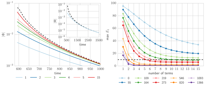
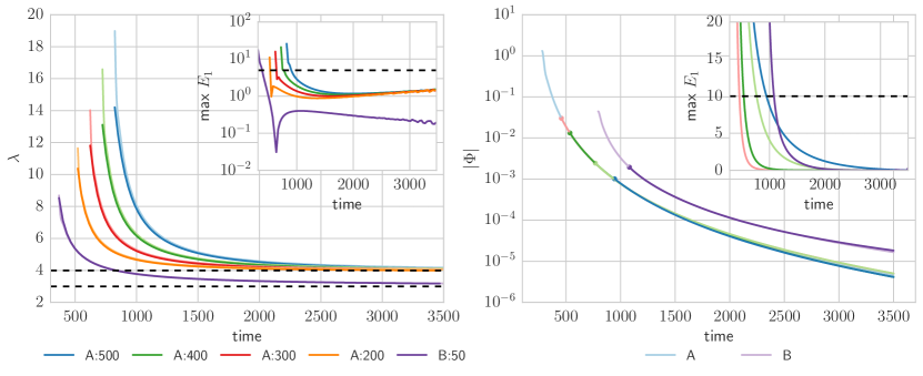
Figure 2: Top row, left: Comparison between the scalar field time-series extracted at $r\simeq 500$ (in dotted line) with those obtained from the approximate Green’s function for a simulation with Gaussian I type initial data. The colors indicate the different number of terms considered in the summation in Eqn. (86). The inset figure shows that at late times, the slowest decaying $t^{-4}$ term dominates. Top row, right: Variation of the maximum $E_{1}$ between $\Phi_{\textrm{b}}$ and $\Phi_{\textrm{gf}}$ at different starting times, mentioned in units of M for Gaussian II type data. Bottom row, left: A comparison between the LPI for two simulations at different observer positions mentioned in the legend, in units of $M$. The inset plots the maximum $E_{1}$ for the corresponding LPI comparison. Bottom row, right: Results of the tail fits to two different types of initial data when considering $q=1,2,3,4$ and $q=4$ in Eqn. (114) respectively. The inset plot shows the variation of the maximum $E_{1}$ with time for the different fits with the dotted line denoting $10\%$. The fits get progressively better as $q$ increases. In both plots, ‘A’ corresponds to a simulation with Gaussian I data and ‘B’ to Gaussian II type data.

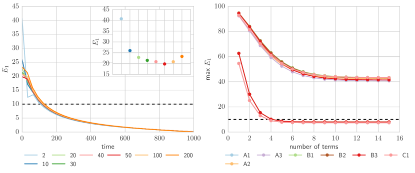
Figure 3: Left: Variation of the pointwise percentage error $E_{1}$ between the numerical signal and the late time Green’s function result as a function of time for scalar field extracted at radii $r\simeq$ $2$, $10$, $20$, $30$, $40$, $50$, $100$ and $200M$ for Gaussian I data. The inset plot shows the values of $E_{1}$ at the beginning of the tail for the same time-series. Right: Variation of the maximum $E_{1}$ with respect to time for an observer at $r\simeq 2M$ with different number of terms in the Green’s function in Eqn. (86) at two starting times for all $7$ simulations. At intermediate starting times, the maximum error can be kept to less than $10\%$ if $5$ or more terms are considered in the Green’s function. The legend shows the three type A, three type B and one type C simulation used in the analysis.

III.3 Tests on tails

We first test the expressions for late time tails using a set of $7$ high-resolution simulations with Gaussian I, II and sine-Gaussian type initial data. For each simulation, the scalar field information is extracted for $10$ different observers outside the event horizon whose positions are approximately at $r\simeq 2$, $10$, $20$, $30$, $40$, $50$, $100$, $200$, $300$, $400$ and  $500M$. As mentioned earlier, care must be taken to place the outer boundary at a sufficiently large radius compared to the position of the observer and the initial ‘pulse’ to ensure that boundary effects do not contaminate the time-series in the region of interest. This problem could be completely avoided by evolving the scalar field in hyperboloidal coordinates. In the following analysis, what we call the ‘tail signal’ starts when the QNM ringing ceases to dominate the signal, and for operational purposes, this starts from the last extremum of the time-series onwards. This signal is then compared with our standalone Green’s function code which computes the low frequency contribution of the branch cut using Eqn. (86), but with a truncated sum. To quantify the disagreement between the numerical data and the Green’s function result, we define a measure of error

$$E_{1}(t,r_{\textrm{o}})=\left|\frac{\Phi_{\textrm{b}}-\Phi_{*}}{\Phi_{\textrm{b}}}\right|\times 100,$$ (112)

which is the percentage error at time $t$ as seen by an observer at $r_{\textrm{o}}$. Here $\Phi_{\textrm{b}}$ is the numerical signal which has $N$ points while $\Phi_{*}$ is $\Phi_{\textrm{gf}}$ or $\Phi_{\textrm{f}}$, the signal computed either from the approximate Green’s function or derived from fitting a model respectively.

One of our aims in this section is to construct a model for the tail signal as a superposition of power laws. To find out the number of terms needed to faithfully represent the numerical result, we generate the first $15$ terms of the approximate Green’s function as in Eqn. (86) and compute the maximum percentage error between $\Phi_{\textrm{b}}$ and $\Phi_{\textrm{gf}}$ while cumulatively adding more terms in $\Phi_{\textrm{gf}}$. Additionally, the starting time for computing the mismatch is varied to compute the maximum $E_{1}$ across early, intermediate and late time tails separately.

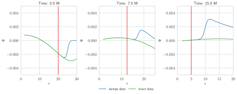
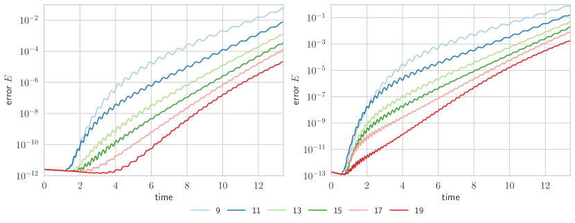
Figure 4: Top row, from left to right: A comparison between the pure QNM solution and the numerical data for the $n=0$ mode at three different times. The left of the vertical red line denotes the region up to which the numerical data and the pure QNM data must agree. Bottom row, from left to right: Convergence plot for $\Phi$ and $\Pi$ respectively for data prepared from the $n=1$ mode with the error computed from Eqn. (116). The colors represent the different resolutions of the simulations.

At very late times, we see that the maximum $E_{1}$ does not vary significantly with the addition of a few terms irrespective of where the observer is located and both can be kept to less than $10\%$. This however becomes progressively worse at earlier times and may be improved by adding more terms in our approximation of the Green’s function as can be seen in the top row, left of Fig. 2. For the simulations considered, the intermediate tail onwards can be described to an accuracy of $<10\%$ error if at least the first $5$ terms are considered in Eqn. (86). This is demonstrated in an example simulation in the top row, right of Fig. 2 and is the rule of thumb followed when building our model.

At very late times, we observe only the effects of the $m=0$ term within Eqn. (86) on the signal. This is reflected in the local power index (LPI) $\lambda$ of the time-series defined as Harms_2013

$$|\Phi|=At^{-\lambda}, \quad\lambda=-\frac{\partial\log|\Phi|}{\partial\log t}.$$ (113)

A comparison between the LPI computed from $\Phi_{\textrm{b}}$ and $\Phi_{\textrm{gf}}$ again shows that they are in good agreement for intermediate times. Generally irrespective of the position of the observer the maximum $E_{1}$ between the numerical and analytically computed $\lambda$ can be kept smaller than $10\%$, and the mismatch is only large at very early times, as can be seen in bottom row, left of Fig. 2. For late times, $\lambda$ approaches $4$ for Gaussian I and sine-Gaussian data and $3$ for Gaussian II data, which is consistent with Price’s law PriceTail . We must note here that the time derivative of the scalar field is only approximately zero at large radii for Gaussian I and sine-Gaussian data, so $\lambda$ must eventually approach $3$ if the simulations are evolved for a much longer time.

We now proceed to fit a sum of tail laws to the data with constant coefficients

$$|\Phi|=\sum_{k=0}^{q}A_{k}t^{-(3+k)}.$$ (114)

While this model is a simplification over the time dependence in Eqn. (86), it should work well for late times. A non-linear least squares fit is performed using the Levenberg-Marquardt algorithm as implemented in the Python package lmfit lmfit at different starting times to obtain the coefficients $A_{k}$. Non-linear fitting algorithms are sensitive to initial conditions and can perform poorly if the $A_{k}$’s are initialized with random values. To initialize the first non-zero coefficient, we make use of the fact that at late times, the slowest decay dominates the signal and is either the $t^{-3}$ term or the $t^{-4}$ term depending on the initial data. While obtaining the first non-zero coefficient is straightforward, it is less clear how to obtain good guesses for the others. Noting that the other tail components contribute significantly at earlier times, we initialize all coefficients with values of the first non-zero coefficient. This empirical approach works remarkably well in practice.

For each time-series, the starting time is shifted over the entire signal and the maximum percentage error is recorded for each position. The maximum $E_{1}$ with respect to time between the fit and the numerical data displays a monotonically decreasing behavior with starting time. The earliest recorded start time at which the maximum $E_{1}$ is less than or equal to $10\%$ is considered the optimal starting time for the fit. The maximum number of terms $q$ in Eqn. (114) is also allowed to vary from $1$ to $11$. More of the signal can be modeled with increasing $q$ until $q$ is equal to $5$. The maximum $E_{1}$ gets worse as $q$ is increased further, and hence the very early part of the signal is not well represented as a linear combination of different power law tails with constant coefficients. A representative fit with different number of terms in the tail model is shown at the bottom row, right of Fig. 2.

Finally, we look at how well the asymptotic expressions perform for non-asymptotic observers. To do this, we compute the pointwise percentage error between $\Phi_{\textrm{b}}$ and $\Phi_{\textrm{gf}}$ for several positions outside the event horizon and find that the beginning of the tail signal always has a considerable error ($>10\%$) irrespective of the simulation and the position of the observer. However, at intermediate times, the percentage error falls beneath $10\%$ and therefore we propose that the asymptotic tail expressions may also be used for observers very close to the event horizon at intermediate and later times. Furthermore, we also look at the maximum percentage error for signals at $r\simeq 2M$ across the $7$ simulations and find that it cannot be kept to under $10\%$ if the entire tail signal is chosen for the analysis. It is only from intermediate time onwards that the error $E_{1}$ can be kept under $10\%$. Fig. 3 left shows the variation of $E_{1}$ between $\Phi_{\textrm{b}}$ and $\Phi_{\textrm{gf}}$ with time while Fig. 3 right shows the maximum percentage error when the fit is performed from the beginning of the tail signal and from intermediate times, for different number of terms in the tail model.

III.4 Tests on QNMs

III.4.1 Results from exact solutions

Looking at the analytically continued solutions $f_{-}$ and $f_{+}$, we see that at QNM frequencies, these solutions are unbounded at spatial infinity. This fact makes it difficult to evolve pure QNM type initial data in our numerical code unless the outer boundary can be treated appropriately. One suggestion is to have time dependent boundary conditions at the outer boundary which can be analytically determined. The alternative is to make the initial data near the outer boundary of the order of machine precision or less by employing a smooth cutoff function,

$$C(r,a,r_{0})=\frac{1}{2}\left(1-\tanh(a(r-r_{0}))\right).$$ (115)

This cutoff changes smoothly from $1$ to $0$ around $r_{0}$, with $C$ being $0.5$ at $r_{0}$. The steepness of this change is controlled by the value of $a$.

The second route is easier to implement and is the one followed here. Our objective in these experiments is two-fold. First we wish to obtain an arbitrarily long ‘ringing time’ for observers close to the event horizon and second to have a ringdown at a specific QNM frequency. This data can be used to obtain an arbitrarily long ringing time of a single QNM, or a superposition of QNMs near the event horizon. Since the ingoing light speed is exactly $1$ in Kerr-Schild coordinates, to obtain a ringing duration of $\Delta t_{\textrm{QNM}}\simeq 20M$, the pure QNM solution and the initial data must match up until at least $r\simeq 22M$. This is achieved in our case by choosing $r_{0}=25M$ and $a=1$ for the $n=0$ mode and $r_{0}=25M$ and $a=2$ for the $n=1$ mode.

A good way to test the correctness of the scalarfield implementation is to perform a convergence test with the initial data built from the exact solution in the region unaffected by the cutoff function. The basic steps for implementing such a test are given below,

1. Generate and evolve the modified QNM data on a Schwarzschild background at $5$ different resolutions or more. For our test, we choose subpatches with $9$ to $19$ points, increasing the number of points by $2$ each time.

2. Compute the pure QNM initial data at a much higher resolution than the highest resolution used for the numerical runs. This ensures that interpolation errors, which can be problematic, do not dominate in the test. We constructed the QNM data from $r\in[1.8,50]$ with $5\cdot 10^{4}$ points or more.

3. Interpolate the exact solution on each bamps subpatch and output at the same times as in our numerical simulations. A comparison of the analytically evolved initial data and the numerical data for the $n=0$ mode at three different times is shown in the top row of Fig. 4.

4. Compute the error $E$ between the numerical result $\Phi_{\textrm{b}}$ and the analytic results $\Phi_{\textrm{e}}$ for the first $P$ subpatches where the data is not affected by the cutoff function

   $$E(t)=\sum_{i=1}^{P}\int_{i}(\Phi_{\textrm{e}}(t,r)-\Phi_{\textrm{b}}(t,r))^{2}dr.$$ (116)

   Here the data on each grid is specified at the Gauss-Lobatto points and the weights for the integration on each grid with $N$ points must be calculated from the Chebshev Gauss-Lobatto numerical quadrature

   $$w_{i}=\begin{cases}\sqrt{1-x^{2}_{i}}({\pi}/{2N}),\ i=0,N,\\ \sqrt{1-x^{2}_{i}}({\pi}/{N}),\ \text{elsewhere},\\ \end{cases}$$ (117)

   where $x_{i}$ for each grid are given by,

   $$x_{i}=-\cos\left(\frac{\pi i}{N-1}\right).$$ (118)

5. Plot the error $E$ as a function of time for each resolution. For the test to be successful, $E$ should decrease with increasing resolution. A convergence test for the $n=1$ mode is shown in the bottom row of Fig. 4.

A comparison between the numerical and analytical solutions at different times show excellent agreement in the region unaffected by the cutoff. We use the matrix pencil Hua and Prony methods BertiDA to fit damped exponentials to the time series data on the horizon. Since the signal is real, we fit two damped exponentials $Ae^{i\omega t+i\phi_{0}}$ for each mode, $\omega$ being the complex QNM frequency. The parameters of the fit provide very accurate numbers for the QNM frequency, namely $0.11043074-0.10485913i$ (with less than $0.01\%$ error) for the $n=0$ mode and $0.0857-0.3472i$ (with less than $0.1\%$ error) for the $n=1$ mode.

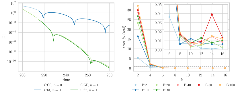
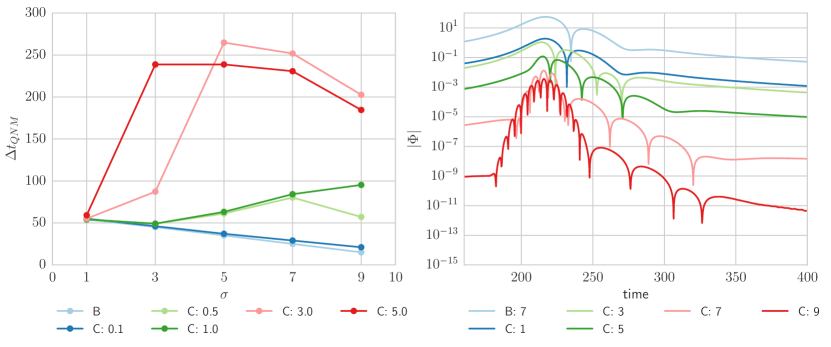
Figure 5: Top row, left: A comparison between the numerical data and the Green’s function result for the $n=0$ and $n=1$ mode for sine-Gaussian initial data. Top row, right: The percentage error in extracting the real part of the $n=0$ QNM frequency from the fit when different number of terms are considered in the fit model in Eqn. (119). The legend specifies the positions of the observer considered, in units of $M$ for a Gaussian II type simulation. The inset plot zooms in a portion of the plot. Bottom row, left: Approximate ringing time for observers at $r\simeq 100M$ calculated from the Green’s function for Gaussian II and sine-Gaussian initial data for different values of $\sigma$. The legend specifies the values of $\omega$ used. Bottom row, right: Variation of QNM ringing from numerical simulations as seen by an observer at $r\simeq 100M$ for Gaussian II and sine-Gaussian initial data ($\omega=1$). The legend specifies the values of $\sigma$ used.

III.4.2 Results from generic data

We now test our expressions for the QNM part of the Green’s function using non-specialized initial data. For this, we use the simulations in section III.3 taking $6$ observers outside the black hole at at $r\simeq 2$, $10$, $20$, $30$, $40$, $50$ and $100M$.

The time-series at each of these points must be cropped to include just the ‘ringing’ part of the signal. To do this, we restrict the signal to the interval between the first extrema during ringing and the start of the ‘tail signal’. During the data analysis, the starting time for the fit is varied over the signal and the time at which the normalized modulus square of the difference between the fit and the numerical data is found to be minimized is chosen as the optimum starting time for the fit.

The model for the fit is chosen to be a linear combination of $k$ damped exponentials

$$\Phi_{\textrm{mp}}=\sum_{j=0}^{k}A_{j}e^{(\alpha_{j}+i\omega_{j})t+i\phi_{j}},$$ (119)

where the fit is performed for the parameters $\{A_{j},\alpha_{j},\omega_{j},\phi_{j}\}$ using the matrix pencil method Hua . For real signals, $k$ is chosen to be an even number and the pencil parameter is kept at one-third the number of points in the time-series rounded off to an integer value. To ensure that the frequencies extracted from the signal are reliable, we check to ensure that the values of $|\omega_{j}|-i|\alpha_{j}|$ which must occur in pairs, do not differ from each other by more than $10^{-4}$ in both the real and imaginary part. Since the algorithm is designed for complex signals in general, $\Phi_{\textrm{mp}}$ may have an imaginary component and this ensures that it is kept small. A summary of the steps to implement this algorithm is provided in BertiDA .

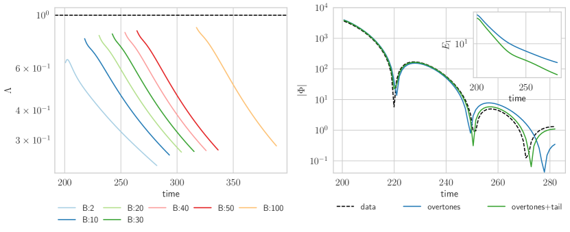
Figure 6: Left: The values of $\Lambda$, defined in Eqn. (122) for different observers located at $r\simeq 2$, $10$, $20$, $30$, $40$, $50$ and $100M$ are less than $1$, showing that the effects of the tail play an important role during QNM ringing, especially at intermediate and late times, since generally $\Lambda$ decreases with increasing time. Right: A comparison of the numerical signal with theoretical contributions from the QNM only and the combined contribution of the QNMs and tail. The inset plot shows the pointwise percentage error in the two cases.

For each time-series, we perform fits with the number of damped exponentials in Eqn. (119) varying from $k=2$ to $16$ and record the fundamental mode frequency. If the above conditions are met, we also record the first overtone. The percentage error for the real and imaginary parts of the extracted frequencies are then calculated for different observers and for different values of $k$. The corresponding contributions from the $n=0,1$ modes are calculated from the Green’s function and compared with the results of the fit.

The Green’s function predicts that the contribution from the overtones is significant during the beginning of the signal, which is why fitting two damped exponentials results in the largest percentage error in the value for the principal QNM frequency. Despite a few exceptions when the percentage error is small, as a general trend the percentage error decreases as the number of exponentials in the fitting model are increased. With only two exponentials in the model, the best value for the $n=0$ mode is obtained by an observer close to the horizon with the percentage error under $10\%$. In general, with the addition of $6$ or more terms in the model, the error for the fundamental mode can be kept within $1\%$ for both the real and imaginary parts, irrespective of the observer chosen. We also compared the $n=0$ mode generated by the fitting algorithm and the Green’s function and found to be in good agreement, with the error between the two amplitudes at the beginning to be $<10\%$ for most cases.

III.4.3 Overtones with generic data

The investigation of overtone modes with generic initial data is less successful. We choose the same set of simulations and perform the data analysis using the same methods as the previous section. It is challenging to reliably extract the first overtone in all cases because some of the extracted frequencies fail to satisfy the consistency test for a pair of damped exponentials mentioned before. In this case, a model with more damped exponentials will not necessarily lead to a more accurate estimation of the first overtone, but more than $4$ damped exponentials are needed for reliable extraction. The accuracy of the frequency extracted is not highly dependent on the position of the observer, although the frequency extracted is seen to be more accurate for observers close to the horizon. As a general rule, the imaginary part of the frequency is extracted more accurately than the real part. Even then, for generic initial data the percentage errors for both the real and imaginary part of the frequency are too large for them to be of real use. The best case we observe for our data set is $<3\%$ error in both the real and imaginary part of the first overtone. The large error or the inability to detect the first overtone can be attributed to the limitations of the fitting algorithm, short duration of ringing and the presence of a significant contribution from the backscattering during intermediate and late ringdown.

The shortcomings of the linear fitting method may be improved by using a non-linear algorithm with an improved model incorporating the tail while the short ringing time may be improved by using specialized initial data which enhances the duration of ringing. All of this is discussed in the rest of the paper. A representative fit for the fundamental mode and the first overtone is shown the top row, left of Fig. 5 while on the top right we show the error in estimating the $n=0$ QNM frequencies for various positions of the observer and various number of terms considered.

III.4.4 QNMs with specialized data

After limited success in extracting overtone modes with generic initial data, we wish to prepare specialized data which allows for more accurate measurement of the first overtone. A naive observation here is that the data analysis algorithm and subsequently the parameter estimation works better with a larger number of ringdown cycles. An elementary way to achieve this is by evolving a pure overtone type initial data. The alternative approach, which we describe here, is to approximate the ringing time from the Green’s function. While it is not possible to infer the parameters of the initial data by specifying a ringing duration $\Delta t_{\textrm{QNM}}$, the converse is easily achieved from combining the results of the QNM and tail components of the Green’s function. The basic prescription is outlined below:

1. The first step to estimate the duration of ringing is to choose a starting time $t_{\textrm{i}}$ for ringing. For an asymptotic observer, this is the time taken by the ingoing part of the initial data to interact with the peak of the scattering potential near the light ring and propagate outwards towards the observer. The starting time can be intuitively approximated as

   $$t_{\textrm{i}} \approx r_{0}+5\sigma+r+4M\log(r-2M)$$

   $$\quad-6M+4M\log M.$$ (120)

   For observers close to the horizon, a more simple expression can be obtained,

   $$t_{\textrm{i}}\approx r_{0}+5\sigma-2M.$$ (121)

   Here $r_{0}$ is the peak of the Gaussian with a standard deviation $\sigma/\sqrt{2}$.

2. An appropriate duration for the search $t_{\textrm{f}}$ is then chosen, assuming that the effects of the tail dominate over the QNM ringing before this time. In our searches, we choose $t_{\textrm{f}}=t_{\textrm{i}}+300M$.

3. The QNM contribution to the signal, upto the first three terms in Eqn. (69) and the tail contribution to the signal, upto the first 15 terms in Eqn. (86) is evaluated over $\left[t_{\textrm{i}},t_{\textrm{f}}\right]$, for a specific choice of initial data.

4. The modulus of the QNM sum amplitude decays linearly and intersects with the tail amplitude at time $t_{\textrm{q}}$, which we shall consider at the end time of ringing. The approximate ringing time is taken to be $\Delta t_{\textrm{QNM}}\approx t_{\textrm{q}}-t_{\textrm{i}}$. Some estimates for the approximate ringing time from the Green’s function are given in the bottom left of Fig. 5.

As a test for this method, we perform a brief comparison between Gaussian II and sine-Gaussian type initial data. For Gaussian II data, we estimate $\Delta t_{\textrm{QNM}}$ for $5$ different values of $\sigma=1,3,5,7,9$. The same is used for sine-Gaussian data with $\omega=0.1,0.5,1,3,5$ for each $\sigma$. In both cases, the Gaussian is centered around $r_{0}=100M$ and the observer is positioned at $r\approx 100M$. We observe an appreciable variation in $\Delta t_{\textrm{QNM}}$ when sine-Gaussians are used, in fact with suitable choice of parameters, $\Delta t_{\textrm{QNM}}\sim 250M$ which is about $5$ times what we can achieve with Gaussian II data. We must note here that although such long duration ringing may be seen by observers far away from the event horizon in principle, it is hardly the case in practice owing to the constraints from numerical noise. This technical problem could be redressed by assigning more memory for floating point numbers in bamps. To illustrate the point that the QNM frequencies can be extracted from the data more reliably, we consider two simulations, one with Gaussian II type data with parameters $A=10^{4}M$, $\sigma=7M$, $r_{0}=100M$ and another with sine-Gaussian data with parameters $A=10^{4}M$, $\sigma=5M$, $r_{0}=100M$, $\omega M=1$. An observer is placed at $r\approx 100M$ and a fit of damped sinusoids is performed on the QNM part of the time-series extracted in both cases. A plot of the signals, as seen in the bottom right of Fig. 5, shows a very short ringdown phase in the first signal, labeled as B:7 while a much longer ringdown phase is observed in the second signal, labeled as C:5. A longer ringdown signal enables QNM frequencies to be estimated more accurately far away from the black hole with some estimates given in table 2.

Simulation	$n$	$\omega_{n}$	$\%$ error
B:7	0	$0.1179-0.1039i$	$(6.71,0.99)$
	1	NA	NA
C:5	0	0.1105-0.1050i	(0.05, 0.06)
	1	0.0912-0.3630i	(5.96, 4.31)

Table 2: Estimated values of the $n=0$ and $n=1$ for generic and special initial data as measured by an observer at $r\simeq 100M$.

In our case, there is an improvement of two orders of magnitude for the $n=0$ mode, which is impressive given that all $l=0$ modes are damped away fairly quickly.

III.4.5 Importance of tails during ringdown

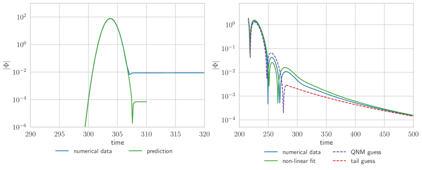
Figure 7: Left: A fit for the scalar field time series as seen by an observer near the horizon ($r\approx 2M$) with the model in Eqn. (123) using the Levenberg-Marquardt algorithm. The separate QNM and tail guesses are also shown. Right: A comparison between the contribution of the high frequency arc to the signal from the approximate Green’s function and the numerical data for Gaussian I type initial data with the observer at $r\simeq 500M$.

We now investigate the effect of the branch cut to the signal during QNM ringing. To do this, we compute the overtone and the approximate tail contribution for the entire duration of the ‘ringing signal’. The tail contribution is approximated by extending the low frequency expressions in Eqn. (86), evaluated up to the first $15$ terms to earlier times and the QNM contribution is computed from the sum of the contribution of the first three modes. We then calculate the difference between the numerical data $\Phi_{\textrm{b}}$ and the mode sum $\Phi_{\textrm{q}}$ and between the numerical data minus the approximate tail contribution $\Phi_{\textrm{t}}$ and the mode sum. The modulus of the ratio of these two quantities

$$\Lambda=\left|\frac{\Phi_{\textrm{b}}-\Phi_{\textrm{t}}-\Phi_{\textrm{q}}}{\Phi_{\textrm{b}}-\Phi_{\textrm{q}}}\right|,$$ (122)

is observed as a function of time. For all simulations considered, $\Lambda$ is seen to be less than $1$ and in general decreases with increasing time. This can be seen in the left of Fig. 6. This demonstrates that the contribution from the tail becomes important during intermediate and late time ringing and should be considered in the fitting model along with the damped sinusoids for better extraction of the QNM frequencies. As a proof of concept, we fit damped sinusoids to $\Phi_{\textrm{b}}-\Phi_{\textrm{t}}$ using the linear fitting strategy described before to $168$ signals and observe an improvement in the percentage error for the principal QNM frequency in $\sim 69\%$ cases while the improvement in measuring the first overtone is seen in $~{}33\%$ cases for generic initial data. On the right of Fig. 6 we show a representative plot where both contributions of the overtones and the tail are considered during ringing.

III.5 Approximation of pre-ringdown

We make a comparison between the leading order contribution from the high frequency arc and the numerical data and find good agreement with the numerics at early times but the flat space approximation rapidly fails at later times. This shortcoming can be redressed by considering higher order terms in the high frequency approximation of the Whittaker functions. In the left of Fig. 7 we display a comparison plot for Gaussian I type data.

IV Discussion and conclusions

Motivated both by gravitational wave astronomy and by pure theory, the principal objective of this paper was to help facilitate, in the near future, a comparison between linear and non-linear perturbation theory by extending the Green’s function approach to arbitrary horizon-penetrating coordinates. This allows us to find the dynamic excitation amplitude of each QNM excited for any observer outside the event horizon. This was achieved by generalizing the computations of DV for QNMs in Eddington-Finkelstein coordinates to arbitrary horizon penetrating coordinates, and computing the exact Green’s function from solutions of the CHE. Under the approximation that the observer is far away from the event horizon, the solutions of the asymptotic form of CHE are just solutions of a Whittaker equation. The resulting expressions for the asymptotic Green’s function are much easier to handle. They were then used to compute the dominant contribution from the high frequency arc as well as the contributions from the branch cut at low, intermediate and high frequencies. The late time contribution from the branch cut gives rise to Price’s tail law. These results were then put to the test using the new scalarfield project inside bamps, in which a single Schwarzschild black hole is perturbed by different configurations of a spherically symmetric massless scalar field.

Besides a verification of our mathematical results, the numerical experiments also show that the first overtone mode may not be reliably extracted from generic initial data for observers far away from the black hole. However, by using specialized initial data we were able to increase the duration of ringing almost threefold, thereby extracting the frequencies of the fundamental mode and the first overtone more accurately. We also found that the branch cut contributes significantly during intermediate and late ringing, and must be taken into account in the data analysis model. It is therefore sensible to consider a data analysis model for QNM ringing which also incorporates the effect of the branch cut, as given for example by,

$$\Phi_{m}=\sum_{j=0}^{2}A_{j}e^{-\alpha_{j}t}\sin(\omega_{j}t+\phi_{j})+\sum_{k=0}^{4}\frac{B_{k}}{t^{3+k}}.$$ (123)

In our experiments with this model we found that at least $3$ damped sinusoids and $5$ tail terms are needed for an accurate representation of the signal. Additionally, the starting time for the signal has to be determined by an additional parameter.

The Levenberg-Marquardt non-linear least squares technique may be used to fit the model to the data. We find, however, that the method may fail to converge if initial guesses for the parameters are far away from their correct values. Our strategy to obtain good parameters for the tail terms is to isolate the tail signal and perform the tail analysis separately while for the QNM parameters, we obtain good initial values with the matrix pencil method. All of these parameters are then used as initial guesses while fitting for the entire signal for different starting times of the fit. In the right of Fig. 7, a demonstration of such a fit is given.

Several improvements are possible on the present approach. While we see that the asymptotic expressions for the tail work well, even for observers close to the event horizon, an exact Green’s function for the branch cut may also be obtained using the solutions of the CHE built along the lines of the MST approach MSTa ; MSTb . Our approximation for the contribution of the high frequency arc fails to account for the subdominant terms for which a more nuanced approach for handling high frequency approximations of the Whittaker function is necessary. It is known that solutions to the Teukolsky master equation can be written down in terms of the confluent Heun equation Fiziev_2010 , so another natural extension to this work would be to consider the spin-$1$ and spin-$2$ cases. Our comparison between the linear results and full non-linear theory is ongoing and will be presented separately.

- (1) Tullio Regge and John A. Wheeler. Stability of a Schwarzschild singularity. Phys. Rev., 108:1063–1069, Nov 1957.
- (2) Frank J. Zerilli. Gravitational field of a particle falling in a Schwarzschild geometry analyzed in tensor harmonics. Phys. Rev. D, 2:2141–2160, Nov 1970.
- (3) C. V. Vishveshwara. Scattering of gravitational radiation by a Schwarzschild black-hole. Nature (London), 227:936–938, August 1970.
- (4) Emanuele Berti, Vitor Cardoso, and Andrei O Starinets. Quasinormal modes of black holes and black branes. Classical and Quantum Gravity, 26(16):163001, 2009.
- (5) Hans-Peter Nollert. Quasinormal modes: The characteristic ‘sound’ of black holes and neutron stars. Classical and Quantum Gravity, 16(12):R159, 1999.
- (6) Kostas D. Kokkotas and Bernd G. Schmidt. Quasi-normal modes of stars and black holes. Living Reviews in Relativity, 2(1):2, Sep 1999.
- (7) R. A. Konoplya and Alexander Zhidenko. Quasinormal modes of black holes: From astrophysics to string theory. Rev. Mod. Phys., 83:793–836, Jul 2011.
- (8) B. P. Abbott et al. Observation of gravitational waves from a binary black hole merger. Phys. Rev. Lett., 116:061102, Feb 2016.
- (9) B. P. Abbott et al. GW151226: Observation of gravitational waves from a 22-solar-mass binary black hole coalescence. Phys. Rev. Lett., 116:241103, Jun 2016.
- (10) B. P. Abbott et al. GW170104: Observation of a 50-solar-mass binary black hole coalescence at redshift 0.2. Phys. Rev. Lett., 118:221101, Jun 2017.
- (11) B. P. Abbott et al. GW170608: Observation of a 19 solar-mass binary black hole coalescence. The Astrophysical Journal Letters, 851(2):L35, 2017.
- (12) B. P. Abbott et al. GW170814: A three-detector observation of gravitational waves from a binary black hole coalescence. Phys. Rev. Lett., 119:141101, Oct 2017.
- (13) B. P. Abbott et al. Multi-messenger observations of a binary neutron star merger. The Astrophysical Journal Letters, 848(2):L12, 2017.
- (14) B. P. Abbott et al. Tests of general relativity with GW150914. Phys. Rev. Lett., 116:221101, May 2016.
- (15) B. P. Abbott et al. Tests of general relativity with GW170817. arXiv e-prints, November 2018.
- (16) T. G. F. Li et al. Towards a generic test of the strong field dynamics of general relativity using compact binary coalescence. Phys. Rev. D, 85:082003, Apr 2012.
- (17) M. Agathos et al. Tiger: A data analysis pipeline for testing the strong-field dynamics of general relativity with gravitational wave signals from coalescing compact binaries. Phys. Rev. D, 89:082001, Apr 2014.
- (18) Jeroen Meidam et al. Parametrized tests of the strong-field dynamics of general relativity using gravitational wave signals from coalescing binary black holes: Fast likelihood calculations and sensitivity of the method. Phys. Rev. D, 97:044033, Feb 2018.
- (19) Werner Israel. Event horizons in static vacuum space-times. Phys. Rev., 164:1776–1779, Dec 1967.
- (20) B. Carter. Axisymmetric black hole has only two degrees of freedom. Phys. Rev. Lett., 26:331–333, Feb 1971.
- (21) Maximiliano Isi, Matthew Giesler, Will M. Farr, Mark A. Scheel, and Saul A. Teukolsky. Testing the no-hair theorem with GW150914. Phys. Rev. Lett., 123:111102, Sep 2019.
- (22) Reinaldo J. Gleiser, Carlos O. Nicasio, Richard H. Price, and Jorge Pullin. Colliding black holes: How far can the close approximation go? Phys. Rev. Lett., 77:4483–4486, Nov 1996.
- (23) Reinaldo J Gleiser, Carlos O Nicasio, Richard H Price, and Jorge Pullin. Second-order perturbations of a Schwarzschild black hole. Classical and Quantum Gravity, 13(10):L117, 1996.
- (24) Carlos O. Nicasio, Reinaldo J. Gleiser, Richard H. Price, and Jorge Pullin. Collision of boosted black holes: Second order close limit calculations. Phys. Rev. D, 59:044024, Jan 1999.
- (25) Reinaldo J. Gleiser, Carlos O. Nicasio, Richard H. Price, and Jorge Pullin. Evolving the Bowen-York initial data for spinning black holes. Phys. Rev. D, 57:3401–3407, Mar 1998.
- (26) Reinaldo J. Gleiser, Carlos O. Nicasio, Richard H. Price, and Jorge Pullin. Gravitational radiation from Schwarzschild black holes: the second-order perturbation formalism. Physics Reports, 325(2):41 – 81, 2000.
- (27) Hirotada Okawa, Helvi Witek, and Vitor Cardoso. Black holes and fundamental fields in numerical relativity: Initial data construction and evolution of bound states. Phys. Rev. D, 89:104032, May 2014.
- (28) Nicolas Sanchis-Gual, Juan Carlos Degollado, Pedro J. Montero, and José A. Font. Quasistationary solutions of self-gravitating scalar fields around black holes. Phys. Rev. D, 91:043005, Feb 2015.
- (29) Nicolas Sanchis-Gual, Juan Carlos Degollado, Paula Izquierdo, José A. Font, and Pedro J. Montero. Quasistationary solutions of scalar fields around accreting black holes. Phys. Rev. D, 94:043004, Aug 2016.
- (30) Robert Benkel, Thomas P. Sotiriou, and Helvi Witek. Dynamical scalar hair formation around a Schwarzschild black hole. Phys. Rev. D, 94:121503, Dec 2016.
- (31) Hiroyuki Nakano and Kunihito Ioka. Second-order quasinormal mode of the Schwarzschild black hole. Phys. Rev. D, 76:084007, Oct 2007.
- (32) Piotr Bizoń, Tadeusz Chmaj, and Andrzej Rostworowski. Late-time tails of a self-gravitating massless scalar field, revisited. Classical and Quantum Gravity, 26(17):175006, Aug 2009.
- (33) Bernd Brügmann. A pseudospectral matrix method for time-dependent tensor fields on a spherical shell. Journal of Computational Physics, 235:216 – 240, 2013.
- (34) David Hilditch, Andreas Weyhausen, and Bernd Brügmann. Pseudospectral method for gravitational wave collapse. Phys. Rev. D, 93:063006, Mar 2016.
- (35) Marcus Bugner, Tim Dietrich, Sebastiano Bernuzzi, Andreas Weyhausen, and Bernd Brügmann. Solving 3D relativistic hydrodynamical problems with weighted essentially nonoscillatory discontinuous Galerkin methods. Phys. Rev. D, 94:084004, Oct 2016.
- (36) David Hilditch, Enno Harms, Marcus Bugner, Hannes Rüter, and Bernd Brügmann. The evolution of hyperboloidal data with the dual foliation formalism: mathematical analysis and wave equation tests. Classical and Quantum Gravity, 35(5):055003, 2018.
- (37) David Hilditch, Andreas Weyhausen, and Bernd Brügmann. Evolutions of centered Brill waves with a pseudospectral method. Phys. Rev. D, 96:104051, Nov 2017.
- (38) Hannes R. Rüter, David Hilditch, Marcus Bugner, and Bernd Brügmann. Hyperbolic relaxation method for elliptic equations. Phys. Rev. D, 98:084044, Oct 2018.
- (39) Andreas Schoepe, David Hilditch, and Marcus Bugner. Revisiting hyperbolicity of relativistic fluids. Phys. Rev. D, 97:123009, Jun 2018.
- (40) Marcus Ansorg and Rodrigo Panosso Macedo. Spectral decomposition of black-hole perturbations on hyperboloidal slices. Phys. Rev. D, 93:124016, Jun 2016.
- (41) Manuela Campanelli, Gaurav Khanna, Pablo Laguna, Jorge Pullin, and Michael P Ryan. Perturbations of the Kerr spacetime in horizon-penetrating coordinates. Classical and Quantum Gravity, 18(8):1543–1554, March 2001.
- (42) Olivier Sarbach and Manuel Tiglio. Gauge-invariant perturbations of Schwarzschild black holes in horizon-penetrating coordinates. Phys. Rev. D, 64:084016, Sep 2001.
- (43) Edward W. Leaver. Spectral decomposition of the perturbation response of the Schwarzschild geometry. Phys. Rev. D, 34:384–408, Jul 1986.
- (44) N. Andersson. Excitation of Schwarzschild black-hole quasinormal modes. Phys. Rev. D, 51:353–363, January 1995.
- (45) Nils Andersson. Evolving test fields in a black-hole geometry. Phys. Rev. D, 55:468–479, Jan 1997.
- (46) Emanuele Berti and Vitor Cardoso. Quasinormal ringing of Kerr black holes: The excitation factors. Phys. Rev. D, 74:104020, Nov 2006.
- (47) Huan Yang, Fan Zhang, Aaron Zimmerman, and Yanbei Chen. Scalar Green function of the Kerr spacetime. Phys. Rev. D, 89:064014, Mar 2014.
- (48) Zhongyang Zhang, Emanuele Berti, and Vitor Cardoso. Quasinormal ringing of Kerr black holes. II. Excitation by particles falling radially with arbitrary energy. Phys. Rev. D, 88:044018, Aug 2013.
- (49) Sam R. Dolan and Adrian C. Ottewill. Wave propagation and quasinormal mode excitation on Schwarzschild spacetime. Phys. Rev. D, 84:104002, Nov 2011.
- (50) Yonghe Sun and Richard H. Price. Excitation of quasinormal ringing of a Schwarzschild black hole. Phys. Rev. D, 38:1040–1052, Aug 1988.
- (51) V.P. Frolov and I.D. Novikov, editors. Black hole physics: Basic concepts and new developments, volume 96. 1998.
- (52) Plamen P Fiziev. Exact solutions of Regge-Wheeler equation and quasi-normal modes of compact objects. Classical and Quantum Gravity, 23(7):2447, 2006.
- (53) Plamen P Fiziev. Classes of exact solutions to the Teukolsky master equation. Classical and Quantum Gravity, 27(13):135001, 2010.
- (54) Plamen P Fiziev. Novel relations and new properties of confluent Heun’s functions and their derivatives of arbitrary order. Journal of Physics A: Mathematical and Theoretical, 43(3):035203, 2010.
- (55) Lionel London, Deirdre Shoemaker, and James Healy. Modeling ringdown: Beyond the fundamental quasinormal modes. Phys. Rev. D, 90:124032, Dec 2014.
- (56) Matthew Giesler, Maximiliano Isi, Mark A. Scheel, and Saul A. Teukolsky. Black hole ringdown: The importance of overtones. Phys. Rev. X, 9:041060, Dec 2019.
- (57) M. Hortacsu. Mathematical Physics: Heun functions and their uses in physics, pages 23–39.
- (58) Plamen Fiziev and Denitsa Staicova. Application of the confluent Heun functions for finding the quasinormal modes of nonrotating black holes. Phys. Rev. D, 84:127502, Dec 2011.
- (59) Dennis Philipp and Volker Perlick. Schwarzschild radial perturbations in Eddington-Finkelstein and Painlevé-Gullstrand coordinates. International Journal of Modern Physics D, 24:1542006, May 2015.
- (60) H.S. Vieira, V.B. Bezerra, and C.R. Muniz. Exact solutions of the Klein-Gordon equation in the Kerr-Newman background and Hawking radiation. Annals of Physics, 350:14 – 28, 2014.
- (61) Plamen P. Fiziev. On the Exact Solutions of the Regge-Wheeler Equation in the Schwarzschild black hole interior. arXiv e-prints, pages gr–qc/0603003, Mar 2006.
- (62) T. A. Ishkhanyan and A. M. Ishkhanyan. Expansions of the solutions to the confluent Heun equation in terms of the Kummer confluent Hypergeometric functions. AIP Advances, 4(8):087132, 2014.
- (63) NIST Digital Library of Mathematical Functions. http://dlmf.nist.gov/, Release 1.0.20 of 2018-09-15. F. W. J. Olver, A. B. Olde Daalhuis, D. W. Lozier, B. I. Schneider, R. F. Boisvert, C. W. Clark, B. R. Miller and B. V. Saunders, eds.
- (64) Sergei Yu. Slavyanov and Wolfgang Lay. Special functions. Oxford Mathematical Monographs. Oxford University Press, Oxford, 2000. A unified theory based on singularities, With a foreword by Alfred Seeger, Oxford Science Publications.
- (65) F.W.J. Olver. Differential equations with irregular singularities; Bessel and confluent Hypergeometric functions. In F.W.J. Olver, editor, Asymptotics and Special Functions, pages 229 – 278. Academic Press, 1974.
- (66) Shuhei Mano, Hisao Suzuki, and Eiichi Takasugi. Analytic solutions of the Teukolsky equation and their low frequency expansions. Progress of Theoretical Physics, 95(6):1079–1096, 1996.
- (67) Shuhei Mano, Hisao Suzuki, and Eiichi Takasugi. Analytic solutions of the Regge-Wheeler equation and the post-Minkowskian expansion. Progress of Theoretical Physics, 96(3):549–565, 1996.
- (68) Marc Casals and Adrian Ottewill. High-order tail in Schwarzschild spacetime. Phys. Rev. D, 92:124055, Dec 2015.
- (69) E. W. Leaver. Solutions to a generalized spheroidal wave equation: Teukolsky’s equations in general relativity, and the two-center problem in molecular quantum mechanics. Journal of Mathematical Physics, 27:1238–1265, May 1986.
- (70) E. W. Leaver. An analytic representation for the quasi-normal modes of Kerr black holes. Proceedings of the Royal Society of London A: Mathematical, Physical and Engineering Sciences, 402(1823):285–298, 1985.
- (71) Plamen Fiziev and Denitsa Staicova. Application of the confluent Heun functions for finding the quasinormal modes of nonrotating black holes. Phys. Rev. D, 84:127502, Dec 2011.
- (72) Nikodem Szpak. Quasinormal mode expansion and the exact solution of the Cauchy problem for wave equations. arXiv e-prints, pages gr–qc/0411050, Nov 2004.
- (73) I. S. Gradshteyn and I. M. Ryzhik. Table of integrals, series, and products. Elsevier/Academic Press, Amsterdam, eighth edition, 2015.
- (74) Richard H. Price. Nonspherical perturbations of relativistic gravitational collapse. I. Scalar and gravitational perturbations. Phys. Rev. D, 5:2419–2438, May 1972.
- (75) Miguel Alcubierre. Initial data. In Introduction to 3+1 Numerical Relativity. Oxford University Press, 2012.
- (76) Thomas W. Baumgarte and Stuart L. Shapiro. In Numerical Relativity: Solving Einstein’s Equations on the Computer. Cambridge University Press, 2010.
- (77) M. Alcubierre, S. R. Brandt, B. Brügmann, D. Holz, E. Seidel, R. Takahashi, and J. Thornburg. Symmetry without symmetry: Numerical simulation of axisymmetric systems using cartesian grids. Int. J. Mod. Phys. D, 10(3):273–289, 2001.
- (78) Frans Pretorius. Numerical relativity using a generalized harmonic decomposition. Class. Quant. Grav., 22:425–451, 2005.
- (79) Enno Harms, Sebastiano Bernuzzi, and Bernd Brügmann. Numerical solution of the 2+1 Teukolsky equation on a hyperboloidal and horizon penetrating foliation of Kerr and application to late-time decays. Classical and Quantum Gravity, 30(11):115013, may 2013.
- (80) Matt Newville et al. lmfit/lmfit-py 0.9.13, April 2019.
- (81) Y. Hua and T. K. Sarkar. Matrix pencil method for estimating parameters of exponentially damped/undamped sinusoids in noise. IEEE Transactions on Acoustics, Speech, and Signal Processing, 38(5):814–824, May 1990.
- (82) Emanuele Berti, Vitor Cardoso, José A. González, and Ulrich Sperhake. Mining information from binary black hole mergers: A comparison of estimation methods for complex exponentials in noise. Phys. Rev. D, 75:124017, Jun 2007.
- (83) Plamen P Fiziev. Classes of exact solutions to the Teukolsky master equation. Classical and Quantum Gravity, 27(13):135001, may 2010.