Bounds for the weight of external data in shrinkage estimation

Abstract

Shrinkage estimation in a meta-analysis framework may be used to facilitate dynamical borrowing of information. This framework might be used to analyze a new study in the light of previous data, which might differ in their design (e.g., a randomized controlled trial (RCT) and a clinical registry). We show how the common study weights arise in effect and shrinkage estimation, and how these may be generalized to the case of Bayesian meta-analysis. Next we develop simple ways to compute bounds on the weights, so that the contribution of the external evidence may be assessed a priori. These considerations are illustrated and discussed using numerical examples, including applications in the treatment of Creutzfeldt-Jakob disease and in fetal monitoring to prevent the occurrence of metabolic acidosis. The target study’s contribution to the resulting estimate is shown to be bounded below. Therefore, concerns of evidence being easily overwhelmed by external data are largely unwarranted.

1 Introduction

In some situations it is useful to support an estimate using additional external evidence, for example, when a small study in the context of a rare disease may be supplemented with data from a clinical registry or electronic health records, or when the result from a meta-analysis may be backed by an analysis in a similar field, e.g., a related but somewhat different population. The involved data contributions then take on different roles, namely, that of a source (the external data) and a target (the data of primary interest). Dynamic borrowing refers to the class of approaches where the apparent, empirical similarity or compatibility of the source and the target is taken into account when judging to what degree the two should be lumped together (Röver and Friede, 2020). Such approaches may be implemented, e.g., via hierarchical models or informative priors; both are actually equivalent to some degree in the context of the normal-normal hierarchical model (NNHM) (Schmidli et al., 2014). Similarly, closely related (or partly equivalent) approaches are given by the bias allowance framework (Welton et al., 2012) or the power prior framework (Ibrahim and Chen, 2000). A recent example of such an approach is given by the early pro-tect trial in paediatric Alport disease, where data from a randomized controlled trial (RCT) were supported by source data from an open-label arm and a clinical registry (Gross et al., 2020).

In the context of dynamic borrowing within the NNHM framework, the flow of information is quite commonly illustrated by quoting weights of data sources as these are combined to a joint estimate. As the eventual estimate may be expressed as a weighted average of the input data, the corresponding weights are a useful means of quantifying the studies’ contributions to or influence on the eventual result (Hedges and Olkin, 1985; Hartung et al., 2008). Analogous weights arise for shrinkage estimates (Raudenbush and Bryk, 1985; Robinson, 1991; Viechtbauer, 2010), and, as we will show below, also in the Bayesian paradigm with prior distributions on effect and heterogeneity parameters.

When combining originally separate data sets in a meta-analysis or using shrinkage estimation, there sometimes is concern that evidence from the target data may be overwhelmed by a much larger set of source data, e.g., when combining a small RCT with a large clinical registry or routine data (e.g. electronic health records) (Weber et al., 2018). In such cases it is instructive to explicate the notion of study contributions by considering their weights. Again, we can see the dynamic nature of the approach in the changing weight of external data with varying data compatibility or discrepancy. It turns out that within the Bayesian framework we can determine the minimum weight of the target study (the RCT in the above example) a priori for a given analysis, and with that we are able to provide more insights into the general behaviour of the meta-analysis procedure. The derived formulas show shrinkage estimation to behave reasonably and also predictably.

In the following, we will review the NNHM, and show how “study weights” arise in effect and shrinkage estimation and how the concept may be extended to the Bayesian framework. Then we take a closer look at the weights’ properties and show how these may be bounded across possible prior settings and/or data realisations. The arguments are illustrated by a numerical study, and the ideas are employed in two example applications involving the joint analysis of a “small” target and a “large” source study, as well as two equally-sized studies. Due to the few-studies setup (Friede et al., 2017b; Röver and Friede, 2020), we will be focusing on Bayesian methods and only in between point out some connections to common analogous frequentist results. We close with a discussion of the findings and their practical implications.

2 The normal-normal hierarchical model (NNHM)

The NNHM models a set of $k$ estimates $y_{i}$ and their standard errors $\sigma_{i}$ as

$$y_{i}|\theta_{i},\sigma_{i}\;\sim\;\mathrm{Normal}(\theta_{i},\sigma_{i}^{2})\mbox{,}$$ (1)

where $\theta_{i}$ are the study-specific effects. The $\theta_{i}$ are not necessarily identical for all studies, but they are also associated with a certain amount of variation, expressed as

$$\theta_{i}|\mu,\tau\;\sim\;\mathrm{Normal}(\mu,\tau^{2})\mbox{.}$$ (2)

The mean parameter $\mu$ is the overall mean effect, while $\tau$ denotes the between-study variability (heterogeneity). As noted elsewhere (Hedges and Olkin, 1985; Hartung et al., 2008; Röver, 2020), marginalizing over the parameters $\theta_{i}$, the model may be written as

$$y_{i}|\mu,\tau,\sigma_{i} \sim \mathrm{Normal}(\mu,\,\sigma_{i}^{2}+\tau^{2})\mbox{.}$$ (3)

The NNHM is a random-effects (RE) model, which in the special case of $\tau=0$ reduces to a fixed-effect (FE) (or common-effect) model. It provides a good approximation for many types of effect measures where measurement uncertainty and between-study variability may be assumed to be (approximately) normally distributed (Jackson and White, 2018). Data analysis may then aim at estimating the overall effect $\mu$ or study-specific effects $\theta_{i}$ (“shrinkage estimation”); in the present investigation, we will mostly be concerned with the latter.

In the following, we will denote vectors of effect estimates $(y_{1},\ldots,y_{k})$ and their standard errors $(\sigma_{1},\ldots,\sigma_{k})$ by $\vec{y}$ and $\vec{\sigma}$, respectively. Furthermore, we will be mostly concerned with the special case of only two studies ($k=2$) and a non-informative (improper) uniform prior for the overall effect ($p(\mu)\propto 1$).

3 Study weights

3.1 Conditional weights

Assuming an (improper) uniform prior for the overall effect $\mu$, the conditional posterior distribution of $\mu$ (given $\tau$) is normal with mean

$$\tilde{\mu}(\tau)\;=\;\mathrm{E}[\mu|\tau,\vec{y},\vec{\sigma}]\;=\;\sum_{i=1}^{k}w_{i}(\tau)\,y_{i}\mbox{,}$$ (4)

where the inverse-variance (IV) weights $w_{j}(\tau)$ are given by

$$w_{j}(\tau)\;=\;\frac{\frac{1}{\sigma_{j}^{2}+\tau^{2}}}{\sum_{i=1}^{k}\frac{1}{\sigma_{i}^{2}+\tau^{2}}}$$ (5)

as in the frequentist framework (Hedges and Olkin, 1985; Hartung et al., 2008; Friede et al., 2017a). A similar formula also applies for a normal prior (Röver, 2020). These two (conditionally conjugate) priors are computationally simple, readily motivated, and because of that reason, probably also the most commonly used priors for $\mu$ for this model. Informative priors might for example be motivated by general plausibility considerations or empirical data (Günhan et al., 2020), or determined through expert elicitation (Hampson et al., 2014; Best et al., 2020).

The conditional posterior of the study-specific effect $\theta_{j}$ (the shrinkage estimate) is also normal with mean $\tilde{\theta}_{j}(\tau)$ depending on $y_{i}$ and $\tilde{\mu}(\tau)$, namely

$$\tilde{\theta}_{j}(\tau)\;=\;\mathrm{E}[\theta_{j}|\tau,\vec{y},\vec{\sigma}]\;=\;b_{j}(\tau)\,y_{j}+\bigl{(}1-b_{j}(\tau)\bigr{)}\,\tilde{\mu}(\tau)$$ (6)

where the corresponding weight (Röver, 2020; Wandel et al., 2017) is

$$b_{j}(\tau)\;=\;\frac{\frac{1}{\sigma_{j}^{2}}}{\frac{1}{\sigma_{j}^{2}}+\frac{1}{\tau^{2}}}\mbox{.}$$ (7)

The formulation in (6) shows to which degree the estimate is shrunk towards the common overall mean $\tilde{\mu}(\tau)$ (depending on the amount of heterogeneity). Equation (6) may be re-written as

$$\tilde{\theta}_{j}(\tau) = \Bigl{[}b_{j}(\tau)+\bigl{(}1-b_{j}(\tau)\bigr{)}w_{j}(\tau)\Bigr{]}\,y_{j}\,+\,\sum_{i\neq j}\Bigl{[}\bigl{(}1-b_{j}(\tau)\bigr{)}\,w_{i}(\tau)\Bigr{]}\,y_{i}$$ (8)

$$= c_{jj}(\tau)\,y_{j}+\sum_{i\neq j}c_{ij}(\tau)\,y_{i}$$ (9)

$$= \sum_{i=1}^{k}c_{ij}(\tau)\,y_{i}$$ (10)

so that the actual shrinkage weights $c_{ij}(\tau)$ (the weight of the $i$th study in the estimate of the $j$th study) become more explicit. In the special case of only two studies ($k=2$), the coefficients $c_{ij}(\tau)$ simplify to

$$c_{11}(\tau)\;=\;\frac{\sigma_{2}^{2}+2\tau^{2}}{\sigma_{1}^{2}+\sigma_{2}^{2}+2\tau^{2}}\mbox{,}\qquad c_{12}(\tau)\;=\;\frac{\sigma_{1}^{2}}{\sigma_{1}^{2}+\sigma_{2}^{2}+2\tau^{2}}\mbox{,}$$ (11)

and analogously for $c_{22}$ and $c_{21}$.

The conditional mean $\tilde{\mu}(\tau)$ commonly also arises in frequentist approaches as an overall effect estimator, where usually a heterogeneity estimate $\hat{\tau}$ is plugged in for $\tau$ (Hedges and Olkin, 1985; Hartung et al., 2008). Similarly, plug-in estimates of $\tilde{\theta}_{j}(\tau)$ are widely used and commonly known as “best linear unbiased prediction (BLUP)” (Raudenbush and Bryk, 1985; Robinson, 1991; Viechtbauer, 2010). The weights ($w_{j}(\tau)$ or $c_{ij}(\tau)$) are then often quoted along with the results in order to illustrate the individual studies’ contributions to the overall result. Note that while weights may be appealing, they still constitute an ultimately somewhat heuristic notion of the concept of a study’s contribution, as these only relate to the posterior expectation. A more complete picture might actually be obtained by considering the corresponding meta-analytic-predictive (MAP) prior (Schmidli et al., 2014), which comprehensively describes the information conveyed by the source study.

3.2 Marginal weights

In a Bayesian multiparameter model, the conditional expectations (of effects $\mu$ or $\theta_{j}$) as derived above are commonly of limited interest; what is usually more interesting are the marginal posterior expectations, as these refer to the posterior distribution integrated over other parameters such as the heterogeneity $\tau$ in the considered model. Marginal posterior expectations here result from the conditional expectations as expected values with respect to the heterogeneity’s marginal posterior distribution $p(\tau|\vec{y},\vec{\sigma})$, i.e.,

$$\mathrm{E}[\mu|\vec{y},\vec{\sigma}]=\mathrm{E}_{p(\tau|\vec{y},\vec{\sigma})}\Bigl{[}\mathrm{E}[\mu|\tau,\vec{y},\vec{\sigma}]\Bigr{]}\;\mbox{ and }\;\mathrm{E}[\theta_{j}|\vec{y},\vec{\sigma}]=\mathrm{E}_{p(\tau|\vec{y},\vec{\sigma})}\Bigl{[}\mathrm{E}[\theta_{j}|\tau,\vec{y},\vec{\sigma}]\Bigr{]}\mbox{.}$$ (12)

In both cases, the conditional expectations result in convex combinations of the form $\sum_{i}\alpha_{i}(\tau)\,y_{i}$ (see Equations (4) and (10)). For convex (or, more generally, linear) combinations, we may re-write the expectations as

$$\mathrm{E}_{p(\tau|\vec{y},\vec{\sigma})}\Bigl{[}\sum_{i}\alpha_{i}(\tau)\,y_{i}\Bigr{]}\;=\;\sum_{i}\mathrm{E}_{p(\tau|\vec{y},\vec{\sigma})}[\alpha_{i}(\tau)]\,y_{i}\mbox{,}$$ (13)

so that it becomes apparent that the marginal expectation may again be expressed as a weighted average of the effects $y_{i}$, where the study weights now arise as the posterior expected weights. These constitute straightforward generalizations of the common conditional weights to the Bayesian context. The weights can be obtained from one-dimensional integrals (expectations) involving the heterogeneity’s marginal posterior distribution and may easily be computed numerically; they are returned by default by the bayesmeta R package (Röver, 2015, 2020).

3.3 Properties

For $\tau=0$ the NNHM reduces to the FE model, in which all study effects $\theta_{i}$ coincide with the overall mean $\mu$. As $\tau$ is varied between the two extremes of $\tau=0$ and $\tau\rightarrow\infty$, several effects may be observed for the conditional weights:

• The IV-weights $w_{j}(\tau)$ move (not necessarily monotonically) from “fixed-effect” weights $w_{j}(0)=\frac{\frac{1}{\sigma_{j}^{2}}}{\sum_{i}\frac{1}{\sigma_{i}^{2}}}$ that depend on the study’s precision towards “average” weights $w_{i}(\infty)=\frac{1}{k}$ where all studies have the same weight.

• The weights $b_{j}(\tau)$ increase monotonically from $0$ towards $1$.

• The shrinkage weights $c_{jj}(\tau)$ (the contribution of the $j$th study to its own shrinkage estimate) increase monotonically from the FE weight towards $1$.

For the conditional expectations, this implies:

• The conditional effect estimate $\tilde{\mu}(\tau)$ moves from the FE estimate towards an unweighted average.

• The conditional shrinkage estimates $\tilde{\theta}_{j}(\tau)$ move from the FE estimate towards the “un-pooled” original estimates $y_{j}$.

These effects are also summarized in Table 1. Posterior expectations of the weights depend on the heterogeneity’s posterior distribution $p(\tau|\vec{y},\vec{\sigma})$. For a uniform effect prior, a given heterogeneity prior $p(\tau)$ and standard errors $\sigma_{i}$, the posterior density is given by

$$p(\tau|\vec{y},\vec{\sigma})\;\propto\;p(\tau)\,f_{\vec{\sigma}}(\tau)\,g_{\vec{y}}(\tau)$$ (14)

with

$$\textstyle g_{\vec{y}}(\tau)\;=\;\exp\Bigl{(}-\frac{1}{2}\Bigl{[}\frac{(y_{1}-\tilde{\mu}(\tau))^{2}}{\sigma_{1}^{2}+\tau^{2}}+\frac{(y_{2}-\tilde{\mu}(\tau))^{2}}{\sigma_{2}^{2}+\tau^{2}}\Bigr{]}\Bigr{)}\;=\;\exp\Bigl{(}-\frac{1}{2}\,\frac{(y_{2}-y_{1})^{2}}{\sigma_{1}^{2}+\sigma_{2}^{2}+2\tau^{2}}\Bigr{)}$$ (15)

(see, e.g., Eqn. (11) in Röver (2020)), where $p(\tau)$ is the heterogeneity’s prior density, and $f_{\vec{\sigma}}(\tau)$ is a lengthier term involving $\tau$ and $\vec{\sigma}$. From (15) one can see that the heterogeneity’s posterior depends on the data ($y_{1}$, $y_{2}$) only via the absolute difference $|y_{2}-y_{1}|$, which in a sense constitutes the “empirical” or “observed” amount of heterogeneity, through the exponential term $g_{\vec{y}}(\tau)$.

A closer look at $g_{\vec{y}}(\tau)$ shows that it always remains between zero and one ($0<g_{\vec{y}}(\tau)\leq 1$). For $y_{2}=y_{1}$, it is constant at $g_{\vec{y}}(\tau)=1$. For a given difference $|y_{2}-y_{1}|>0$, it takes its minimum at $\tau=0$ and then increases monotonically with $\tau$. For any given $\tau$ it decreases monotonically in $|y_{2}-y_{1}|$. One might think of $g_{\vec{y}}(\tau)$ as “ruling out” smaller $\tau$ values in the heterogeneity posterior and pushing the posterior mode towards higher $\tau$ values as $|y_{2}-y_{1}|$ increases.

The functional form of the posterior (15) implies that for increasing $|y_{2}-y_{1}|$ the resulting marginal heterogeneity posterior becomes stochastically larger (Shaked and Shanthikumar, 2007); see also the appendix for a derivation. When varying the prior distribution $p(\tau)$ in (14), we may to some extent also predict the effect on the heterogeneity posterior: in particular, choosing a stochastically larger heterogeneity prior will imply a stochastically larger posterior as well (see also the appendix).

Table 1: Effects on several expressions when varying the heterogeneity $\tau$ between its extremes.

		heterogeneity extreme
expression		$\quad\tau=0$	$\quad\tau\rightarrow\infty$
inverse-variance (IV) weight $w_{j}(\tau)$	(4)	FE weight $\Bigl{(}\frac{\sigma_{j}^{-2}}{\sum_{i}\sigma_{i}^{-2}}\Bigr{)}$	average weight $\bigl{(}\frac{1}{k}\bigr{)}$
weight $b_{j}(\tau)$	(6)	$0$	$1$
shrinkage weight $c_{jj}(\tau)$	(10)	FE weight	$1$
conditional overall mean $\tilde{\mu}(\tau)$	(4)	FE estimate	unweighted average
conditional shrinkage estimate $\tilde{\theta}_{j}(\tau)$	(6)	FE estimate	original estimate $y_{j}$

4 Bounds for the study weights

4.1 Lower bounds

The above conditions imply that we can derive bounds for the shrinkage weights. As mentioned previously, concerns are sometimes raised that the target estimates may be overwhelmed by the source data, i.e., that certain weights may become too small (Weber et al., 2018). In the following, we will describe the conditions under which we can derive lower bounds on weights, i.e., where we can make sure that weights remain above a certain minimum. Important consequences for the weights, valid quite generally or for certain heterogeneity priors $p(\tau)$, are derived below. Note that while we assume the standard errors $\sigma_{i}$ to be given (a common assumption to be made in meta-analysis or study design considerations), the data (estimates $y_{i}$) or the prior ($p(\tau)$) may be varied.

4.2 A study’s minimum contribution to its own shrinkage estimate: the “FE weight”

The (conditional) shrinkage weight $c_{jj}(0)$, i.e. the $j$th study’s contribution to its own shrinkage estimate evaluated at $\tau=0$, constitutes a lower bound for the posterior mean weights. Any heterogeneity prior $p(\tau)$ may attach prior probability to $\tau$ values larger than zero, for which the weights are only increasing. These “FE weights” may simply be computed as the common study weights in a fixed-effect meta-analysis. This property holds independent of the actual data ($y_{i}$) or the heterogeneity prior ($p(\tau)$).

4.3 Minimum posterior mean shrinkage weight: the “coincidence weight”

For any prior distribution $p(\tau)$, the coincidence case of $y_{1}=y_{2}$ is the data realisation yielding the lowest possible posterior mean shrinkage weight. Any data with $|y_{2}-y_{1}|>0$ will imply a stochastically larger heterogeneity posterior that will (due to monotonicity of weights $c_{jj}(\tau)$ as a function of $\tau$) lead to larger posterior mean shrinkage weights. The coincidence weights may simply be computed by performing the meta-analysis with the data ($y_{1}$ and $y_{2}$) substituted by two identical numbers. This property holds independent of the data ($y_{i}$) and for any given heterogeneity prior ($p(\tau)$).

4.4 Stochastically ordered priors and their posterior mean weights

Considering stochastically ordered families of heterogeneity priors allows to vary the posterior mean shrinkage weight. For properly chosen stochastically smaller priors, the posterior mean may approach the FE weight, while for stochastically larger priors the posterior mean weight may approach 100%. An obvious, simple way to yield a stochastically ordered family of prior distributions for the heterogeneity is by using (or introducing) a scale parameter (Mood et al., 1974, Sec. VII.6.2). An example would be given by varying the scale parameter within the half-normal family of prior distributions (Röver et al., 2020). This property holds for given data ($y_{i}$) and a stochastically ordered family of heterogeneity priors ($p(\tau)$).

5 Numerical illustration

In order to demonstrate the shrinkage weights’ properties, we consider an illustrative case motivated by a scenario involving a log-odds-ratio (log-OR) endpoint, analogous to the simulation scenario discussed by Röver and Friede (2020). For a study of size $n_{i}$ featuring two treatment arms and a binary endpoint, the results may be summarized in a $2\!\times\!2$ contingency table. Assuming an even distribution of events and non-events across table cells implies a log-OR estimate with a standard error of approximately $\frac{4}{\sqrt{n_{i}}}$ (Röver, 2020). Considering a combination of a “small” and a “large” study with sizes $n_{1}=25$ and $n_{2}=400$ then leads to standard errors of $\sigma_{1}=0.8$ and $\sigma_{2}=0.2$, respectively. We will then derive the smallest RCT’s shrinkage estimate (for the study-specific effect $\theta_{1}$) that is of course primarily informed by $y_{1}$, but supported by the external data $y_{2}$. The present case of $\sigma_{1}\gg\sigma_{2}$ is the kind of setting in which we expect to see larger gains from shrinkage estimation, and this is exactly where using historical data is the most attractive in practice.

For the analysis, we choose a half-normal heterogeneity prior with scale $0.5$ (HN(0.5)), which constitutes a conservative choice for the present scenario (Friede et al., 2017a; Röver et al., 2020). For illustration purposes, we also utilize a (stochastically larger) HN(1.0) prior. We then fix the target $y_{1}$ (arbitrarily) at zero and vary the source $y_{2}$ in order to investigate the effect on the resulting shrinkage estimates and weights.

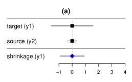
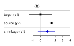
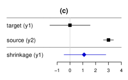
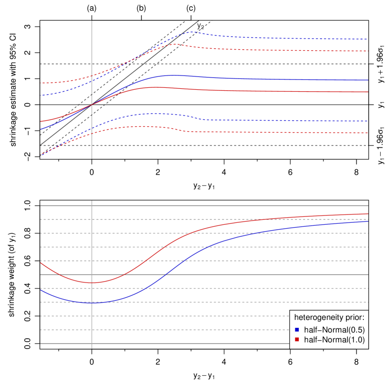
Figure 1: Effect of varying the difference between quoted estimates ($y_{2}-y_{1}$) on the first shrinkage estimate (for $\theta_{1}$). The top row shows three data examples of (a) coinciding and (b)–(c) increasingly diverging estimates, along with the resulting shrinkage estimate for the target study. The second row illustrates the estimates across the continuum of increasing $y_{2}$ values relative to the “plain” interval ($y_{1}\pm 1.96\sigma_{1}$). The bottom panel shows the posterior mean shrinkage weight ($\mathrm{E}[c_{11}(\tau)|\vec{y},\vec{\sigma}]$) for the first study, based on two different priors and for varying $y_{2}-y_{1}$. Note that $y_{2}-y_{1}=0$ constitutes the “coincidence case”.

Fig. 1 illustrates estimates’ and weights’ dependence on the difference between estimates ($y_{1}$ and $y_{2}$). The top row of forest plots shows three example cases of (a) coinciding target and source estimates, (b) some moderate and (c) larger discrepancy between the two; the resulting shrinkage estimate for the target is shown in blue. The second row shows the posterior means of $\theta_{1}$ (solid lines) and the corresponding 95% CIs (dashed lines) across the continuum of source data values. At the top of the plot the three cases (a)–(c) are marked, and the blue lines correspond to the estimates also shown above. The red lines show analogous estimates, but corresponding to a (stochastically larger) HN(1.0) prior. Note that “large” $|y_{2}-y_{1}|$ values (here e.g. $|y_{2}-y_{1}|>1.96(\sigma_{1}+\sigma_{2})=1.96$) would imply non-overlapping CIs for source and target studies (as in case (c)), which in reality may mean that estimates would not actually be pooled at all. The practically most relevant bit of the plot is hence in the neighbourhood of zero.

Finally, the bottom plot shows the posterior expected weights to illustrate the first (target) study’s contribution to its own shrinkage estimate. The minimum (for both heterogeneity priors) is attained in the “coincidence case” (a) of $y_{2}-y_{1}=0$; e.g., for the HN(0.5) prior the coincidence weight is at $29\%$. Increasing the observed effect difference $|y_{2}-y_{1}|$ (i.e., the “observed heterogeneity”) then yields increasing weights for $y_{1}$, implying less borrowing from the source. In cases (b) and (c), the shrinkage weight amounts to $38\%$ and $63\%$, respectively. Also, the choice of a stochastically larger prior, here realized by a larger scale parameter in the same familiy of distributions, leads to larger weights for $y_{1}$, for any $|y_{2}-y_{1}|$, including the minimum at $|y_{2}-y_{1}|=0$. The first study’s absolute minimum shrinkage weight, the “FE weight”, in this case is at $c_{11}(0)=\frac{\sigma_{1}^{2}}{\sigma_{1}^{2}+\sigma_{2}^{2}}=\frac{1}{17}=5.9\%$.

Note that while “$y_{1}=y_{2}$” constitutes a “worst case” in a certain sense (leading to the lowest shrinkage weight), it also still is the most desirable case, in the sense that this is when the data are in agreement and one would expect to learn the most from the source study.

6 Applications

6.1 Creutzfeldt-Jakob example

Table 2: Data from Varges et al. (2017) on an observational and a randomized study investigating the effect of doxycycline on survival in Creutzfeldt-Jakob disease (CJD).

		patients		log(HR)
$i$	study	treatment	control	$y_{i}$	$\sigma_{i}$
$1$	observational	55	33	$-0.499$	$0.249$
$2$	randomized	07	05	$-0.173$	$0.631$

A small randomized controlled trial (RCT) was conducted in order to investigate the effect of doxycycline on survival in patients suffering from Creutzfeldt-Jakob disease (CJD). In this ultra rare condition, only 12 patients could be recruited, and so data from an observational study were considered as complementing evidence (Varges et al., 2017). Both studies quote estimated hazard ratios (HRs), and these estimates along with their standard errors are jointly analyzed in a meta-analysis; the data are also shown in Table 2. With the focus being on the evidence from the RCT, a shrinkage estimate for this study is derived (Röver and Friede, 2020). Both studies are in agreement, suggesting a beneficial treatment effect, while the absolute effect magnitude is larger for the observational data.

Since the larger observational study provides a much more precise estimate (smaller standard error), one might fear that the randomized evidence will be overwhelmed by the external data in a joint analysis. The FE weight in this case amounts to $c_{22}(0)=\frac{\sigma_{2}^{2}}{\sigma_{1}^{2}+\sigma_{2}^{2}}=13.5\%$; this would be the RCT’s weight in an FE analysis, and it constitutes a lower bound on the RCT’s weight for any data realization ($y_{1}$, $y_{2}$) or any heterogeneity prior ($p(\tau)$).

For a log-HR, we may then assume a half-normal prior with scale 0.5 (HN(0.5)) for the heterogeneity (Friede et al., 2017a; Röver and Friede, 2020; Röver et al., 2020). For this prior, we get a minimum posterior mean weight (coincidence weight) for the randomized study of $38.9\%$, which may already be considered reassuringly large, in view of the sample sizes involved and compared to the FE weight. Any data realization ($y_{1}$, $y_{2}$) will hence yield an eventual weight $\geq 38.9\%$ for the RCT. Also, a larger scale of the heterogeneity prior (i.e., a larger expected amount of heterogeneity) will increase the minimum weight for $y_{2}$; e.g., a HN(1.0) prior would yield a minimum expected shrinkage weight of $52.1\%$. For the actual data (Table 2), we then get a weight of $39.5\%$, slightly above the minimum, for the RCT. Table 3 shows weights and estimates corresponding to the two different heterogeneity priors. In both cases, the actual weights are not far from their minimum value, and for both analyses there is a sizeable gain in precision for the shrinkage estimate when compared to the original estimate ($y_{2}$, $\sigma_{2}$) alone.

Table 3: Estimates for the CJD example. For different heterogeneity priors (HN(0.5) or HN(1.0)), the corresponding minimum (coincidence) weight is given, as well as the resulting weight for the actual data along with the corresponding shrinkage estimates. The very last line shows the estimate based only on $y_{2}$ and $\sigma_{2}$ for comparison.

	mean weight		effect estimate $\theta_{2}$
$\tau$ prior	minimum	actual	mean	95% CI
HN(0.5)	38.9%	139.5%	$-0.370$	[$-1.157$, $0.477$]
HN(1.0)	52.1%	153.1%	$-0.326$	[$-1.232$, $0.664$]
		(100.0%)	$-0.173$	([$-1.410$, $1.064$])

6.2 Metabolic acidosis example

A gynaecological RCT investigated whether fetal monitoring using cardiotocography (CTG) combined with ECG ST-segment analysis (ST) reduced the occurrence of metabolic acidosis, compared to CTG alone (Westerhuis et al., 2007). Here the relative risk (RR) of metabolic acidosis comparing the two treatment groups is of interest. When analyzing the data, evidence from an earlier, similar RCT (Amer-Wåhlin et al., 2001) may be utilized to support parameter estimation. This example data set was originally investigated by Rietbergen et al. (2011); the corresponding data are shown in Table 4.

Table 4: Data from Rietbergen et al. (2011) on two gynaecological RCTs investigating whether fetal monitoring using cardiotocography (CTG) combined with ECG ST-segment analysis was associated with a reduced risk of metabolic acidosis, compared to CTG alone.

		treatment		control		log(RR)
$i$	study	events	total	events	total	$y_{i}$	$\sigma_{i}$
$1$	Amer-Wåhlin (2001)	15	2159	31	2079	$-0.764$	$0.313$
$2$	Westerhuis (2007)	20	2827	30	2840	$-0.401$	$0.287$

Primary interest focuses on the more recent target study by Westerhuis et al. (2007) and on a shrinkage estimate of its study-specific effect $\theta_{2}$. The two trials are of roughly comparable size (5667 vs. 4238 participants), and from the “FE weight” of $c_{22}(0)=\frac{\sigma_{2}^{2}}{\sigma_{1}^{2}+\sigma_{2}^{2}}=54.3\%$ one can already see that the second study will definitely contribute the majority of weight when estimating its own effect $\theta_{2}$.

For a log-RR, we may again use a half-normal prior with scale 0.5 for the heterogeneity (Friede et al., 2017a; Röver et al., 2020); this yields a minimum (coincidence) mean shrinkage weight of $72.5\%$. A larger heterogeneity prior scale again leads to an increased shrinkage weight; e.g., for a HN(1.0) prior, the minimum weight is at $78.7\%$.

Table 5: Estimates for the metabolic acidosis example. For different heterogeneity priors (HN(0.5) or HN(1.0)), the corresponding minimum (coincidence) weight is given, as well as the resulting weight for the actual data along with the corresponding shrinkage estimates. The very last line shows the estimate based only on $y_{2}$ and $\sigma_{2}$ for comparison.

	mean weight		effect estimate $\theta_{2}$
$\tau$ prior	minimum	actual	mean	95% CI
HN(0.5)	72.5%	174.0%	$-0.495$	[$-0.986$, $0.005$]
HN(1.0)	78.7%	180.5%	$-0.472$	[$-0.983$, $0.051$]
		(100.0%)	$-0.401$	([$-0.964$, $0.163$])

Table 5 shows the corresponding weights and estimates. Compared to the previous example, the precision gain is not quite as large here.

7 Conclusions

Bayesian meta-analysis provides a transparent means for extrapolation or borrowing of strength from external data (Röver and Friede, 2020). Also within a Bayesian inference framework, study weights for overall and shrinkage effect estimates may be derived as posterior expected weights, for any number of studies $k$. The FE weights (conditional on $\tau\!=\!0$) constitute the absolute minimum shrinkage weights across all heterogeneity priors and data realizations. In case of $k\!=\!2$ studies, the heterogeneity posterior depends on the data only via the absolute difference in both estimates ($|y_{2}-y_{1}|$). A larger difference leads to a stochastically larger heterogeneity posterior. When the estimates coincide, i.e. $y_{2}=y_{1}$, the smallest possible shrinkage weight for a given heterogeneity prior (across all possible data realizations) is obtained. Concerning the choice of heterogeneity prior, a stochastically larger prior leads to a stochastically larger posterior, and with that to increased (minimum and actual) shrinkage weights.

The above findings have important implications for the weightings that may occur within a meta-analysis. The shrinkage weight is bounded below (irrespective of the prior and data) by the FE weight. For any particular given prior, the (posterior mean) shrinkage weight is also bounded below across possible data realisations by the “coincidence weight”. Having a bound on the weight effectively means bounding the “leverage” of the external data for the shrinkage estimate. A lower bound of, say, 50% means that the resulting shrinkage estimate will not move more than halfway from the effect $y_{i}$ towards the external data in case of near-concordant evidence. For greater discrepancies, the target study’s weight will even be larger, or conversely, the influence of the source data will be smaller.

The FDA Guidance on “Leveraging existing clinical data for extrapolation to pediatric uses of medical devices”(U.S. Department of Health and Human Services , Food and Drug Administration (FDA)(2016), HHS) for example elaborates on issues commonly encountered in extrapolation endeavours. One concern raised here is the exchangeability assumption (3) commonly made in hierarchical models. In the common case of only $k\!=\!2$ studies, however, the same model (as far as shrinkage estimation is concerned) may alternatively be motivated via the reference model (Röver and Friede, 2020). This is similar to the bias allowance model framework (Welton et al., 2012), where the target study is estimating the parameter of interest “directly”, while the source is associated with a potential bias term of unknown direction and magnitude. Moreover, the advantages of using (informative) priors on the heterogeneity parameter are acknowledged in the guidance document, in particular as this facilitates dynamical borrowing based on the empirically observed compatibility of source and target data.

We would like to encourage consideration of minimum weights as a diagnostic tool of the evidence constitution and of implications of prior settings for a given or anticipated data scenario. The study of weights should, however, not be used for guiding the selection of the heterogeneity prior. The choice of prior should primarily be driven by considerations of prior information on between-study variability. Different amounts on heterogeneity might however be anticipated in different contexts — e.g., in the two examples discussed above, greater heterogeneity may be plausible between observational and randomized data than for the case of two RCTs (Röver et al., 2020).

A closely related approach to investigating the contributions of data sources to a joint analysis works via the consideration of effective sample sizes (ESS) (Neuenschwander et al., 2020). Target and source data may be assessed based on their “share” of the total sample size, and also the effect of heterogeneity on the resulting MAP prior may be quantified via prior maximum sample sizes (Neuenschwander et al., 2010). Robustification of a MAP prior may be achieved by implementing a mixture of vague and informative prior components (Schmidli et al., 2014). In case the source data’s weight is considered too large, a simple remedy might be to artificially inflate its associated standard error, similarly to the idea behind a power prior approach (Ibrahim and Chen, 2000). Alternatively, the target sample size might also be increased, in case that is an option. For an overviev of approaches to downweighting of external data, see also Viele et al. (2014).

The considerations which provide some insights into the inner workings of shrinkage estimation facilitate diagnostics even before considering actual data. A requirement is that the standard errors ($\sigma_{i}$) need to be known beforehand. Quite often these may be approximated based on a unit information standard deviation (UISD) and the sample size (Kass and Wasserman, 1995; Röver et al., 2020). The need to make assumptions about anticipated standard errors is a common issue in similar design-of-experiment contexts (Cohen, 1988). Fears of external evidence “overruling” the target data (Weber et al., 2018) may be unwarranted, or may be checked before carrying out the target study, as the NNHM behaves predictably and reasonably within a Bayesian analysis. Potential problems arise or are amplified when using frequentist methods: the concerningly common occurrence of zero heterogeneity estimates means that analyses may fall back to an FE approach, which here is the least cautious or least conservative analysis. For the case of few studies, the probability of obtaining a zero heterogeneity estimate is alarmingly high — approaching 50% even for moderate amounts of heterogeneity (Friede et al., 2017a), which may actually render frequentist heterogeneity estimation for small $k$ a somewhat questionable exercise. Within a Bayesian framework, marginalisation over the plausible range of heterogeneity values will lead to a more conservative behaviour. In summary, with the target study’s contribution to the resulting Bayesian shrinkage estimate being bounded below, concerns of evidence being easily overwhelmed by external source data can be addressed a-priori, and may be shown to be largely unwarranted.

Conflicts of interest

The authors have declared no conflict of interest.

ORCID

Christian Röver: 0000-0002-6911-698X
Tim Friede: 0000-0001-5347-7441

Appendix A Appendix

A.1 Stochastic ordering of heterogeneity posteriors

Consider two parameter sets $\vec{y}_{a}$ and $\vec{y}_{b}$ for which $0\leq|y_{a;2}-y_{a;1}|<|y_{b;2}-y_{b;1}|$. Then the ratio of the heterogeneity’s marginal posterior densities is given by (cf. (14))

$$\frac{p(\tau|\vec{y}_{b},\vec{\sigma})}{p(\tau|\vec{y}_{a},\vec{\sigma})}\;=\;\frac{c_{\vec{y}_{b}}\,p(\tau)\,g_{\vec{y}_{b}}(\tau)}{c_{\vec{y}_{a}}\,p(\tau)\,g_{\vec{y}_{a}}(\tau)}\;=\;\frac{c_{\vec{y}_{b}}}{c_{\vec{y}_{a}}}\;\frac{g_{\vec{y}_{b}}(\tau)}{g_{\vec{y}_{a}}(\tau)}\;\propto\;\frac{g_{\vec{y}_{b}}(\tau)}{g_{\vec{y}_{a}}(\tau)}\mbox{,}$$ (16)

where $c_{\vec{y}_{a}}$ and $c_{\vec{y}_{b}}$ are the densities’ normalizing constants, and the where the latter ratio of “$g_{\vec{y}}(\tau)$” terms is monotonically increasing in $\tau$. With that, condition (C) in Lehmann (1955) is fulfilled, and the posterior corresponding to $\vec{y}_{b}$ is stochastically larger than the one associated with $\vec{y}_{a}$.

A.2 Stochastic ordering of posteriors for different priors

Consider two heterogeneity priors with densities $p_{1}(\tau)$ and $p_{2}(\tau)$ where $p_{2}$ is stochastically larger than $p_{1}$. A posterior distribution constitutes a special case of a “weighted distribution” (Mȩczarski, 2015). For the posterior distributions corresponding to $p_{1}$ and $p_{2}$ follows that these will inherit the same stochastic ordering (Bartoszewicz and Skolimowska, 2006).

A.3 R code for CJD example

# specify data:
cjd <- cbind.data.frame("study"   =c("observational", "randomized"),
                        "logHR"   =c(-0.499, -0.173),
                        "logHR.se"=c(0.249, 0.631))

# analyze:
library("bayesmeta")
bm <- bayesmeta(y=cjd$logHR, sigma=cjd$logHR.se, labels=cjd$study,
                tau.prior=function(t){dhalfnormal(t, scale=0.5)})

# show posterior mean shrinkage weights:
bm$weights.theta
# show shrinkage estimates:
bm$theta

# derive FE weights (percentages, using "metafor" library):
weights(rma.uni(yi=cjd$logHR, sei=cjd$logHR.se, slab=cjd$study,
                measure="GEN", method="FE"))
# alternatively, compute directly:
cjd$logHR.se^-2 / sum(cjd$logHR.se^-2)

# determine coincidence (minimum) posterior mean weights:
bayesmeta(y=c(0,0), sigma=cjd$logHR.se, labels=cjd$study,
          tau.prior=function(t){dhalfnormal(t,scale=0.5)})$weights.theta

References

- Amer-Wåhlin et al. (2001) Amer-Wåhlin, I., Hellsten, C., Norén, H., Herbst, A., Kjellmer, I., Lilja, H., Lindoff, C., Månsson, M., Olofsson, P., Sundström, A.-K. and Maršál, K. (2001). Cardiotocography only versus cardiotocography plus ST analysis of fetal electrocardiogram for intrapartum fetal monitoring: a Swedish randomised controlled trial. The Lancet 358, 534–538.
- Bartoszewicz and Skolimowska (2006) Bartoszewicz, J. and Skolimowska, M. (2006). Preservation of classes of life distributions and stochastic orders under weighting. Statistics & Probability Letters 76, 587–596.
- Best et al. (2020) Best, N., Dallow, N. and Montague, T. (2020). Prior elicitation. In E. Lesaffre, G. Baio and B. Boulanger, editors, Bayesian Methods in Pharmaceutical Research, chapter 5, pages 87–109. Chapmann & Hall / CRC.
- Cohen (1988) Cohen, J. (1988). Statistical power analysis for the behavioural sciences. Routledge, New York, 2nd edition.
- Friede et al. (2017a) Friede, T., Röver, C., Wandel, S. and Neuenschwander, B. (2017a). Meta-analysis of few small studies in orphan diseases. Research Synthesis Methods 8, 79–91.
- Friede et al. (2017b) Friede, T., Röver, C., Wandel, S. and Neuenschwander, B. (2017b). Meta-analysis of two studies in the presence of heterogeneity with applications in rare diseases. Biometrical Journal 59, 658–671.
- Gross et al. (2020) Gross, O., Tönshoff, B., Weber, L. T., Pape, L., Latta, K., Fehrenbach, H., Lange-Sperandio, B., Zappel, H., Hoyer, P., Staude, H., König, S., John, J., U. und Gellermann, Hoppe, B., Galiano, M., Hoecker, B., Ehren, R., Lerch, C., Kashtan, C. E., Harden, M., Boeckhaus, J. and Friede, T. (2020). A multicenter, randomized, placebo-controlled, double-blind phase 3 trial with open-arm comparison indicates safety and efficacy of nephroprotective therapy with ramipril in children with Alport’s syndrome. Kidney International 97, 1275–1286.
- Günhan et al. (2020) Günhan, B. K., Röver, C. and Friede, T. (2020). Random-effects meta-analysis of few studies involving rare events. Research Synthesis Methods 11, 74–90.
- Hampson et al. (2014) Hampson, L. V., Whitehead, J., Eleftheriou, D. and Brogan, P. (2014). Bayesian methods for the design and interpretation of clinical trials in very rare diseases. Statistics in Medicine 33, 4186–4201.
- Hartung et al. (2008) Hartung, J., Knapp, G. and Sinha, B. K. (2008). Statistical meta-analysis with applications. John Wiley & Sons, Hoboken, NJ, USA.
- Hedges and Olkin (1985) Hedges, L. V. and Olkin, I. (1985). Statistical methods for meta-analysis. Academic Press, San Diego, CA, USA.
- Ibrahim and Chen (2000) Ibrahim, J. G. and Chen, M.-H. (2000). Power prior distributions for regression models. Statistical Science 15, 46–60.
- Jackson and White (2018) Jackson, D. and White, I. R. (2018). When should meta-analysis avoid making hidden normality assumptions? Biometrical Journal 60, 1040–1058.
- Kass and Wasserman (1995) Kass, R. E. and Wasserman, L. (1995). A reference Bayesian test for nested hypotheses and its relationship to the Schwarz criterion. Journal of the American Statistical Association 90, 928–934.
- Lehmann (1955) Lehmann, E. L. (1955). Ordered families of distributions. The Annals of Mathematical Statistics 26, 399–419.
- Mȩczarski (2015) Mȩczarski, M. (2015). Stochastic orders in the Bayesian framework. Collegium of Economic Analysis Annals 37, Instytut Ekonometrii, Szkoła Główna Handlowa w Warszawie (Institute of Econometrics, Warsaw School of Economics), Warsaw. URL https://EconPapers.repec.org/RePEc:sgh:annals:i:37:y:2015:p:339-360.
- Mood et al. (1974) Mood, A. M., Graybill, F. A. and Boes, D. C. (1974). Introduction to the theory of statistics. McGraw-Hill, New York, 3rd edition.
- Neuenschwander et al. (2010) Neuenschwander, B., Capkun-Niggli, G., Branson, M. and Spiegelhalter, D. J. (2010). Summarizing historical information on controls in clinical trials. Clinical Trials 7, 5–18.
- Neuenschwander et al. (2020) Neuenschwander, B., Weber, S., Schmidli, H. and O’Hagan, A. (2020). Predictively consistent prior effective sample sizes. Biometrics 76, 578–587.
- Raudenbush and Bryk (1985) Raudenbush, S. W. and Bryk, A. S. (1985). Empirical Bayes meta-analysis. Journal of Educational and Behavioural Statistics 10, 75–98.
- Rietbergen et al. (2011) Rietbergen, C., Klugkist, I., Janssen, K. J. M., Moons, K. G. M. and Hoijtink, H. J. A. (2011). Incorporation of historical data in the analysis of randomized therapeutic trials. Contemporary Clinical Trials 32, 848–855.
- Robinson (1991) Robinson, G. K. (1991). That BLUP is a good thing: The estimation of random effects. Statistical Science 6, 15–32.
- Röver (2015) Röver, C. (2015). bayesmeta: Bayesian random-effects meta analysis. R package. URL: http://cran.r-project.org/package=bayesmeta.
- Röver (2020) Röver, C. (2020). Bayesian random-effects meta-analysis using the bayesmeta R package. Journal of Statistical Software 93, 1–51.
- Röver et al. (2020) Röver, C., Bender, R., Dias, S., Schmid, C. H., Schmidli, H., Sturtz, S., Weber, S. and Friede, T. (2020). On weakly informative prior distributions for the heterogeneity parameter in Bayesian random-effects meta-analysis. arXiv preprint 2007.08352 URL http://www.arxiv.org/abs/2007.08352.
- Röver and Friede (2020) Röver, C. and Friede, T. (2020). Dynamically borrowing strength from another study. Statistical Methods in Medical Research 29, 293–308.
- Schmidli et al. (2014) Schmidli, H., Gsteiger, S., Roychoudhury, S., O’Hagan, A., Spiegelhalter, D. and Neuenschwander, B. (2014). Robust meta-analytic-predictive priors in clinical trials with historical control information. Biometrics 70, 1023–1032.
- Shaked and Shanthikumar (2007) Shaked, M. and Shanthikumar, J. G. (2007). Stochastic orders. Springer-Verlag, New York.
- U.S. Department of Health and Human Services , Food and Drug Administration (FDA)(2016) (HHS) U.S. Department of Health and Human Services (HHS), Food and Drug Administration (FDA) (2016). Leveraging existing clinical data for extrapolation to pediatric uses of medical devices. Guidance for Industry and Food and Drug Administration Staff. URL https://www.fda.gov/media/91889/download.
- Varges et al. (2017) Varges, D., Manthey, H., Heinemann, U., Ponto, C., Schmitz, M., Schulz-Schaeffer, W. J., Krasnianski, A., Breithaupt, M., Fincke, F., Kramer, K., Friede, T. and Zerr, I. (2017). Doxycycline in early CJD – a double-blinded randomized phase II and observational study. Journal of Neurology, Neurosurgery and Psychiatry 88, 119–125.
- Viechtbauer (2010) Viechtbauer, W. (2010). Conducting meta-analyses in R with the metafor package. Journal of Statistical Software 36.
- Viele et al. (2014) Viele, K., Berry, S., Neuenschwander, B., Amzal, B., Chen, F., Enas, N., Hobbs, B., Ibrahim, J. G., Kinnersley, N., Lindborg, S., Micallef, S., Roychoudhury, S. and Thompson, L. (2014). Use of historical control data for assessing treatment effects in clinical trials. Pharmaceutical Statistics 13, 41–54.
- Wandel et al. (2017) Wandel, S., Neuenschwander, B., Röver, C. and Friede, T. (2017). Using phase II data for the analysis of phase III studies: an application in rare diseases. Clinical Trials 14, 277–285.
- Weber et al. (2018) Weber, K., Hemmings, R. and Koch, A. (2018). How to use prior knowledge and still give new data a chance? Pharmaceutical Statistics 17, 329–341.
- Welton et al. (2012) Welton, N. J., Sutton, A. J., Cooper, N. J., Abrams, K. R. and Ades, A. E. (2012). Evidence synthesis for decision making in healthcare. Wiley, Chichester, UK.
- Westerhuis et al. (2007) Westerhuis, M. E. M. H., Moons, K. G. M., van Beek, E., Bijvoet, S. M., Drogtrop, A. P., van Geijn, H. P., van Lith, J. M. M., Mol, B. W. J., Nijhuis, J. G., Oei, S. G., Porath, M. M., Rijnders, R. J. P., Schuitemaker, N. W. E., van der Tweel, I., Visser, G. H. A., Willekes, C. and Kwee, A. (2007). A randomised clinical trial on cardiotocography plus fetal blood sampling versus cardiotocography plus ST-analysis of the fetal electrocardiogram (STAN) for intrapartum monitoring. BMC Pregnancy and Childbirth 7, 13.