Impact of non-normal error distributions
on the benchmarking and ranking
of Quantum Machine Learning models

Abstract

Quantum machine learning models have been gaining significant traction within atomistic simulation communities. Conventionally, relative model performances are being assessed and compared using learning curves (prediction error vs. training set size). This article illustrates the limitations of using the Mean Absolute Error (MAE) for benchmarking, which is particularly relevant in the case of non-normal error distributions. We analyze more specifically the prediction error distribution of the kernel ridge regression with SLATM representation and $L_{2}$ distance metric (KRR-SLATM-L2) for effective atomization energies of QM7b molecules calculated at the level of theory CCSD(T)/cc-pVDZ. Error distributions of HF and MP2 at the same basis set referenced to CCSD(T) values were also assessed and compared to the KRR model. We show that the true performance of the KRR-SLATM-L2 method over the QM7b dataset is poorly assessed by the Mean Absolute Error, and can be notably improved after adaptation of the learning set.

¹ Institut de Chimie Physique, UMR8000, CNRS, Université Paris-Saclay, 91405 Orsay, France.
Contact: Pascal.Pernot@universite-paris-saclay.fr

² Institute of Physical Chemistry and National Center for Computational Design and Discovery of Novel Materials (MARVEL), Department of Chemistry, University of Basel, Klingelbergstrasse 80, 4056 Basel, Switzerland.

³ Laboratoire de Chimie Théorique, CNRS and Sorbonne Universités, 75252 Paris, France.

1 Introduction

For users to appreciate the accuracy of a computational chemistry method, one should ideally provide them some statistics enabling to estimate easily the probability to get errors below a threshold corresponding to their requirements. As usual for physical measurements, the most simple statistic would be a prediction uncertainty attached to a method $u(M)$ [1].

If the distribution of residual errors for a benchmark dataset is zero-centered normal, statistics such as the mean absolute error (MAE), the root mean squared deviation (RMSD) or the 95^th quantile of the absolute errors distribution ($Q_{95}$) are redundant and can be used to infer $u(M)$: $u(M)\simeq\mathrm{RMSD}=\sqrt{\pi/2}\mathrm{MAE}\simeq 0.5Q_{95}$. If it is not normal, more information is necessary to provide the user with probabilistic diagnostics [2]. It is therefore primordial to test the normality of the distribution and, in case of non-normality, to consider data transformations that might get the distribution closer to normality. For instance, the use of intensive properties [3, 2], the choice between errors or relative errors [4], and the correction of trends [1] might have a notable impact.

The previous analysis has been applied to computational chemistry methods, but to our knowledge, the error distributions of ML algorithms have not be scrutinized for their ability to deliver a reliable prediction uncertainty, and the general use of the MAE as a benchmark statistic for ML methods [5, 6] has to be evaluated. A problem arises notably when comparing methods with different error distribution shapes, as MAE-based ranking might become arbitrary, occulting important considerations about the risk of large errors for some of the methods [2, 7] .

This is the main topic of the present paper, where we analyze the prediction errors for effective atomization energies of QM7b molecules calculated at the level of theory CCSD(T)/cc-pVDZ by the kernel ridge regression with CM and SLATM representations and $L_{2}$ distance metric [6]. The ML error distributions are compared with the ones obtained from computational chemistry methods (HF and MP2) on the same reference dataset.

In the next section, we present the statistical tools we use to characterize error sets. These are then applied to the HF, MP2, CM-L2 and SLATM-L2 error sets (Section 3). The strong non-normality of the SLATM-L2 errors is then scrutinized and the systems having large errors are analyzed as outliers. The impact on the prediction errors distribution of including these outliers in the learning set is evaluated. The main findings are discussed in Section 4.

2 Statistical methods

Statistical benchmarking of a method $M$ is based on the estimation of errors ($E_{M}=\left\{e_{M,i}\right\}_{i=1}^{N}$) for a set of $N$ calculated ($C_{M}=\left\{c_{M,i}\right\}_{i=1}^{N}$) and reference data ($R=\left\{r_{i}\right\}_{i=1}^{N}$), where

$$e_{M,i}=r_{i}-c_{M,i}$$ (1)

In the present study, reference data are calculated by a quantum chemistry method, and uncertainty on the calculated and reference values are considered to be negligible before the errors.

2.1 Normality assesment

Reliable use of statistical tests of normality require typically at least $N=100$ points [8, 9]. For a given sample size, the Shapiro-Wilk $W$ statistics has been shown to have good properties [8], and it is used in this study. The values of $W$ range between 0 and 1, and values of $W\simeq 1$ are in favor of the normality of the sample. If $W$ lies below a critical value $W_{c}$ depending on the sample size and the chosen level of type I errors $\alpha$ (typically 0.05), the normality hypothesis cannot be assumed to hold [9].

It might also be useful to assess normality by visual tools: normal quantile-quantile plots (QQ-plots) [4], where the quantiles of the scaled and centered errors sample is plotted against the theoretical quantiles of a standard normal distribution (in the normal case, all points should lie over the unit line); or comparison of the histogram of errors with a gaussian curve having the same mean, estimated by the mean signed error (MSE), and same standard deviation, estimated by the RMSD.

Two other statistics are helpful in characterizing the departure from normality. The skewness (Skew), or third standardized moment of the distribution, quantifies its asymmetry (Skew = 0 for a symmetric distribution). The kurtosis (Kurt), or fourth standardized moment, quantifies the concentration of data in the tails of the distribution. Kurtosis of a normal distribution is equal to 3; distributions with excess kurtosis (Kurt > 3) are called leptokurtic; those with Kurt < 3 are named platykurtic.

For error distributions which are non symmetric (Skew $\neq 0$), quantifying the accuracy by a single dispersion-related statistic is not reliable, and one should provide probability intervals or accept to loose information on the sign and use a statistic based on absolute errors, such as $Q_{95}$ presented below.

For platykurtic and leptokurtic error distribution, the normal probabilistic interpretation of dispersion statistics such as the RMSD is lost, and one should rely on dispersion measures providing explicit probability coverage, such as $u_{95}$ recommended in the thermochemistry literature [10]. $u_{95}$ is an enlarged uncertainty which enables to define a symmetric 95 % probability interval around the estimated value. If the distribution is also skewed, one cannot rely on a symmetric interval based on $u_{95}$. A major problem with leptokurtic error distributions is that the excess of data in the tails is related to a risk of large prediction errors, that cannot be appreciated from the usual MAE or RMSD statistics. A solution is again to use $Q_{95}$ (Section 2.2).

For ranking studies, problems might occur when comparing distribution with different shapes, which might lead to conflict between different ranking statistics [2]. A striking example is provided below (Section 3).

2.2 Empirical Cumulative Distribution Function and related statistics

Pernot and Savin [2] have shown that the non-normality of error distributions prevents the probabilistic interpretation of usual benchmark statistics. However, direct probabilistic information can be extracted from the empirical cumulative distribution function (ECDF) of absolute errors $\epsilon_{i}=|e_{i}|$

$$C(\eta)=\frac{1}{N}\sum_{i=1}^{N}\mathbf{1_{\epsilon_{i}\leq\eta}}$$ (2)

where $\eta$ is a threshold value to be chosen, and $\mathbf{1}_{x}$ is the indicator function, with value 1 if $x$ is true and 0 otherwise.

Two statistics based on the ECDF have been proposed as fulfilling the needs of end-users to choose a method suited to their purpose:

• $C(\eta)$ is the probability that the absolute errors lie below a chosen threshold $\eta$, such as the “chemical accuracy” [2]. A user can define his own needs and accordingly pick methods with a high value of $C(\eta)$.

• $Q_{95}$, the 95^th percentile of the absolute error distribution, gives the amplitude of errors that there is a 5% probability to exceed [2]. The choice of this specific percentile was based on several considerations. When the error distribution is normal, $Q_{95}$ is identical to the enlarged uncertainty $u_{95}$ recommended for thermochemical calculations and data [10]. Besides, $Q_{95}$ is much less sensitive to outliers than the maximal error, or even $Q_{99}$ for small datasets. Thakkar et al. [11] proposed a similar statistic ($P_{90}$) based on the 90^th percentile.

As mentioned previously, the use of such probabilistic scores for non-normal distributions relieves the ambiguity attached to the MAE and RMSD. For instance, in all the cases of error sets that Pernot and Savin [2, 7] have studied previously, the probability for an absolute error to be larger than the MAE lied between 0.2 and 0.45 (it should be about 0.42 for a zero-centered normal distribution). The small values are typically associated with skewed and leptokurtic distributions. Several cases have also been observed where two methods have similar MAE values and very different probabilities of large errors, due to their different error distributions.

This non-ambiguity is essential if one wants to assess a risk of large prediction errors. Note that the transition from descriptive statistics to predictive statistics for risk assesment requires further constraints on the reference dataset and error distributions. Ideally, the reference dataset has to be representative enough to cover future prediction cases and there should be no notable trend in the errors with respect to the calculated values by the method of interest (in the statistical prediction framework, the predictor variable is the calculated value of a property, from which one wants to infer a credible interval for its true value).

Several statistical trend correction methods have been proposed in the computational chemistry literature, from the simple scaling of the calculated values [12, 13], or linear corrections [14, 15, 1, 4, 16], to more complex, ML-based corrections, such as $\Delta$-ML [17, 18, 6] or Gaussian Processes [19].

2.3 Outliers identification

There is no unique method to identify outliers for a non-normal distribution. One might, for instance, use visual tools, such as QQ-plots [4], or automatic selection tools, such as selecting points for which the absolute error is larger than the 95-th percentile ($Q_{95}$), or another percentile corresponding to a predefined error threshold.

In cases where the errors distribution seems heterogeneous, one can attempt to analyze it as a mixture of normal distributions. One might for instance use a bi-normal fit

$$\mathscr{E}(x)=\sum_{i=1}^{2}w_{i}\mathcal{N}(x;\mu_{i},\sigma_{i})$$ (3)

where $\mathcal{N}(x;\mu,\sigma)$ is a normal distribution of $x$ with mean value $\mu$ and standard deviation $\sigma$. Outliers are then defined as the points which lie outside of a $\mu_{1}\pm n\times\sigma_{1}$ interval, where $\mu_{1}$ and $\sigma_{1}$ are the parameters of the most concentrated component. The enlargement factor $n$ should be chosen large enough to exclude as much points from this component as possible, but small enough to capture enough points of the wider component to enable tests of chemical or physical hypotheses.

2.4 Implementation

All calculations have been made in the R language [20], using several packages, notably for bootstrap (boot [21]), skewness and kurtosis (moments [22]) and mixture analysis (mixtools [23, 24]). Bootstrap estimates are based on 1000 draws. The R implementation of the Shapiro-Wilk test (function shapiro.test) has a limit of dataset size at 5000 [8]. For the large datasets used in the application, 5000 points are randomly chosen to evaluate $W$.

The code and datasets to reproduce the tables and figures of this article are available at Zenodo (https://doi.org/10.5281/zenodo.3733272). The datasets can also be analyzed with the ErrView code (https://doi.org/10.5281/zenodo.3628489), or its web interface (http://upsa.shinyapps.io/ErrView).

3 Application

The data are issued from the study by Zaspel et al. [6]. The effective atomization energies ($E^{*}$) for the QM7b dataset [25], for 7211 molecules up to 7 heavy atoms (C, N, O, S or Cl) are available for several basis sets (STO-3g, 6-31g, and cc-pVDZ), three quantum chemistry methods (HF, MP2 and CCSD(T)) and four machine learning algorithms (CM-L1, CM-L2, SLATM-L1 and SLATM-L2). The ML methods have been trained over a random sample of 1000 CCSD(T) energies (learning set), and the test set contains the prediction errors for the 6211 remaining systems [6]. We consider here the results for the cc-pVDZ basis set and the CM-L2 and SLATM-L2 methods. Besides, the errors for HF and MP2 have been estimated on the same reference data set as for the ML methods. They provide an interesting contrast in terms of error distribution.

Methods	MAE		MSE		RMSD		$Q_{95}$		$C(\eta)$		Skew		Kurt		$W$
	(kcal/mol)								$\eta=1$ kcal/mol						$W_{c}=0.9993$
HF	2.	38(3)	0.	06(4)	3.	13(4)	6.	1(1)	0.	273(6)	-0.	69(7)	5.	1(3)	0.	970(4)
MP2	1.	31(1)	0.	00(2)	1.	67(2)	3.	35(5)	0.	461(6)	-0.	07(3)	3.	33(6)	0.	9961(8)
CM-L2	10.	1(1)	-0.	0(2)	13.	2(2)	26.	2(4)	0.	071(3)	0.	05(7)	4.	3(3)	0.	990(3)
SLATM-L2	1.	26(3)	0.	13(3)	2.	44(8)	4.	7(1)	0.	651(6)	0.	8(5)	29.	(3)	0.	70(2)
lc-HF	2.	29(3)	0.	0	2.	97(4)	5.	87(8)	0.	285(6)	-0.	46(6)	4.	3(2)	0.	985(3)
lc-MP2	1.	28(1)	0.	0	1.	61(1)	3.	18(5)	0.	470(6)	0.	09(3)	3.	14(6)	0.	9983(5)
lc-CM-L2	10.	1(1)	0.	0	13.	1(2)	26.	4(4)	0.	071(3)	0.	09(7)	4.	4(3)	0.	990(3)
lc-SLATM-L2	1.	27(3)	0.	0	2.	44(8)	4.	7(1)	0.	650(6)	0.	8(5)	28.	(3)	0.	71(2)
SLATM-L2(-o)	0.	85(1)	0.	06(2)	1.	20(2)	2.	71(4)	0.	690(6)	-0.	04(5)	4.	8(1)	0.	968(3)
SLATM-L2(+o)	0.	83(1)	0.	05(2)	1.	20(2)	2.	49(5)	0.	713(6)	-0.	1(1)	8.	1(5)	0.	940(7)
SLATM-L2(+r)	0.	95(2)	-0.	01(2)	1.	89(8)	3.	15(8)	0.	743(6)	0.	4(10)	46.	(7)	0.	65(3)

Table 1: Error summary statistics on effective atomization energies for the QM7b dataset. All calculations are done with the cc-pvdz basis set, and the reference data are CCSD(T) values. Methods with a ’lc-’ prefix include linear correction. For the meaning of the -o, +o and +r suffixes, see Sections 3.3 and 3.4. MAE: mean absolute/unsigned error; MSE: mean signed error; RMSD: root mean squared deviation; $Q_{95}$: 95^th percentile of the absolute errors distribution; Skew, Kurt: skewness and kurtosis of the errors distribution; $C(\eta)$: probability of absolute errors below $\eta=1$ kcal/mol; $W$: Shapiro-Wilk normality statistic. For a sample of size 5000, the critical value is $W_{c}=0.9993$ at the 0.05 level. The normality hypothesis is rejected if $W<W_{c}$. Standard uncertainties estimated by bootstrap are reported in parenthetical notation.

3.1 Error statistics and distributions

Summary statistics and their uncertainty have been estimated by bootstrap [26]. They are reported in Table 1. In this part, one concentrates on the unmodified methods, HF, MP2, CM-L2, and SLATM-L2. Considering MAE alone, one might conclude that SLATM-L2 produces slightly smaller errors than MP2 and a significant improvement over all other methods. MSE tells us that there is no important bias when compared to the MAE or RMSD (all distributions are nearly centered on zero). It is striking that MP2 has a smaller RMSD than SLATM-L2. As the RMSD is often taken as an estimator of prediction uncertainty [1], this contradicts the MAE ranking.

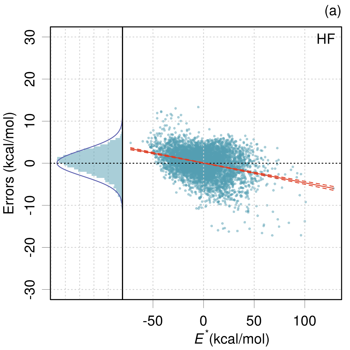
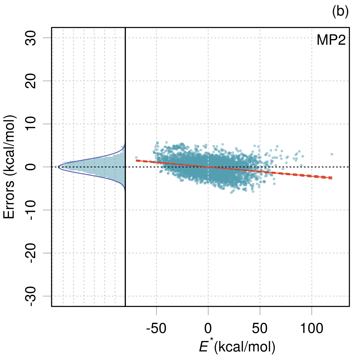
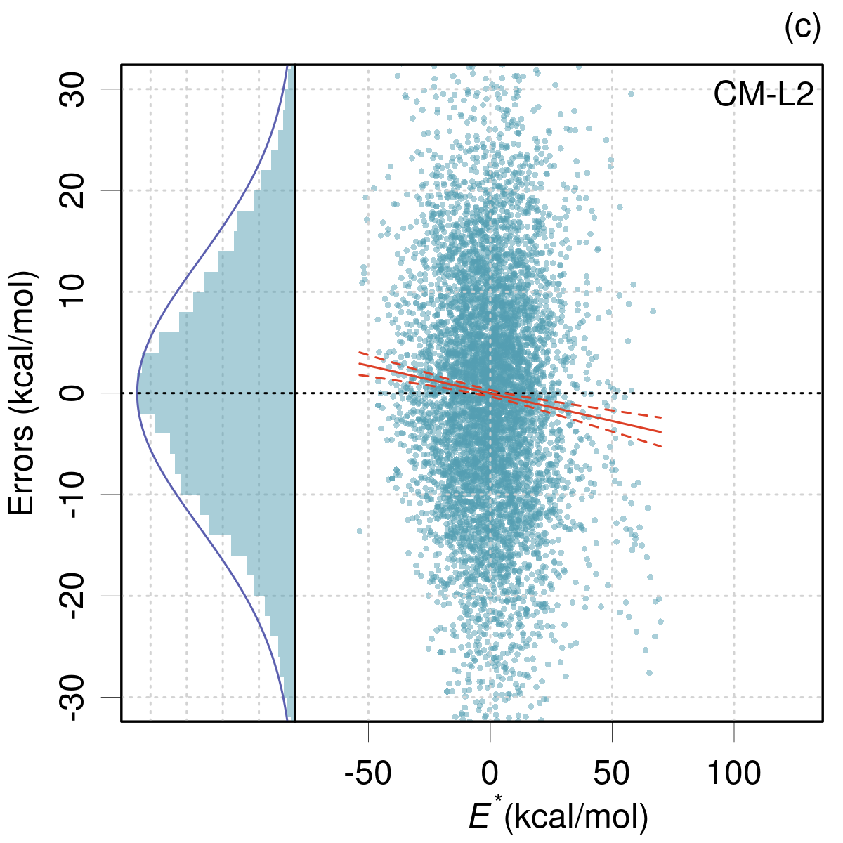
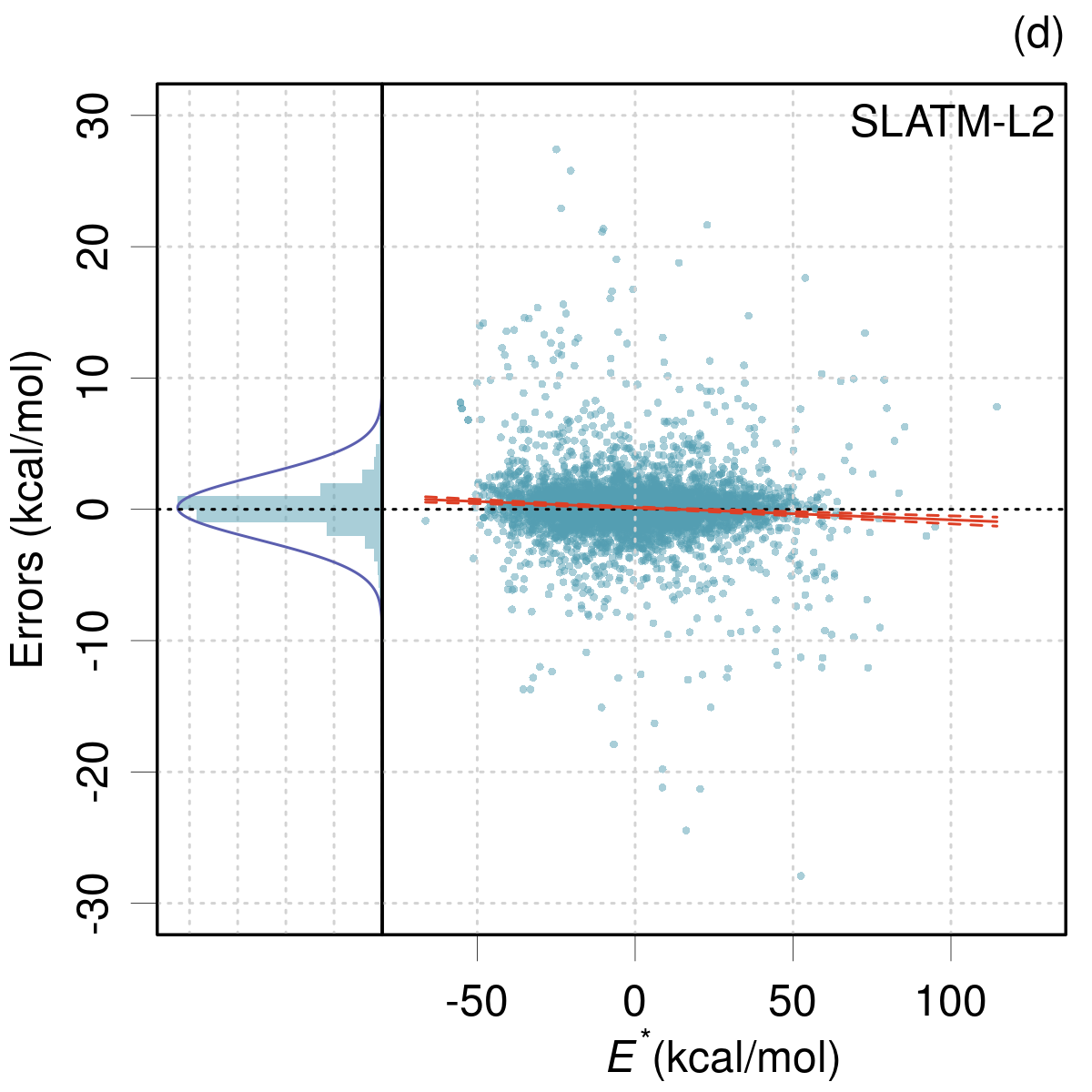
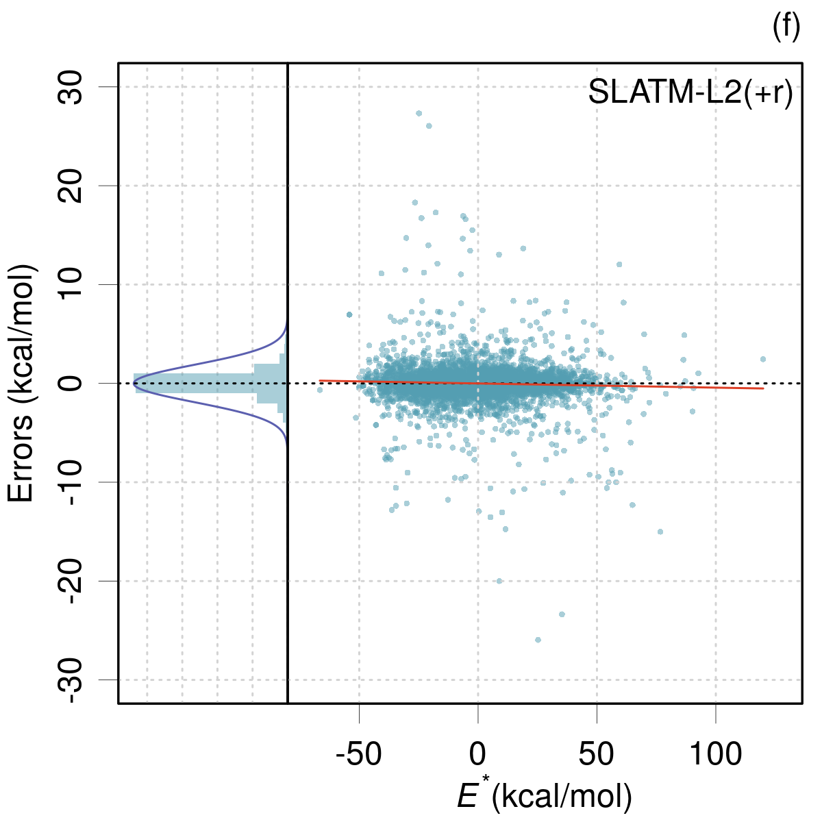
Figure 1: Error distributions for the effective atomization energies $E^{*}$ with respect to CCSD(T) of (a) HF, (b) MP2 (c) CM-L2,(d) SLATM-L2, (e) SLATM-L2(+o) and (f) SLATM-L2(+r). In each sub-figure, the left panel presents the histogram of the errors, with its fit by a normal distribution, and the right panel a scatterplot of the errors vs. the calculated value by the corresponding method. The red lines represent the linear trend with its 95 % confidence interval, obtained by ordinary least squares linear regression.

This is also a strong clue that not all the error distributions are normal. In the case of normal distributions, and considering that MSE$\simeq 0$, the RMSD should confirm the MAE ranking ($RMSD\simeq\sqrt{\pi/2}*MAE$ for a zero-centered normal distribution). Indeed, the Shapiro-Wilk normality test rejects the normality of all the error sets, with a critical value $W_{c}=0.9993$ for $N=5000$ and a type I error rate of 0.05. However the $W$ statistic shows that MP2 is much closer to normal ($W=0.9961$) than SLATM-L2 ($W=0.71$). This is confirmed by the kurtosis, with a very large value for SLATM-L2 (29) whereas for MP2 the value (3.33) is much closer to the value for a normal distribution (3.0). HF and CM-L2 are also leptokurtic (Kurt > 3), but much less than SLATM-L2.

The large kurtosis value indicates that the SLATM-L2 error distribution presents tails much heavier than for a normal distribution. This excess in large errors can be appreciated with $Q_{95}$, which informs us that 5 % of the absolute errors are above 3.3 kcal/mol for MP2 and 4.7 kcal/mol for SLATM-L2. Despite a smaller MAE, one has thus a non-negligible risk to get larger errors by SLATM-L2 than by MP2. Note that in parallel with large errors, there is an excess in small errors: we estimated that the probability to have absolute errors smaller than the RMSD, $C(2.44)$, is 0.9 for SLATM-L2, when it should be 0.67 for a normal distribution.

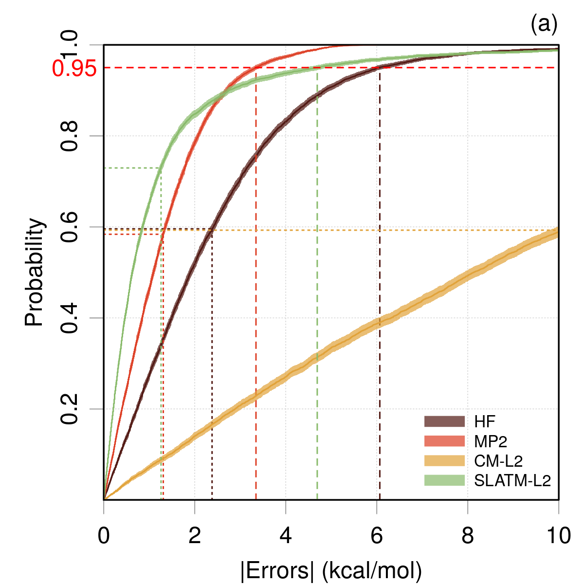
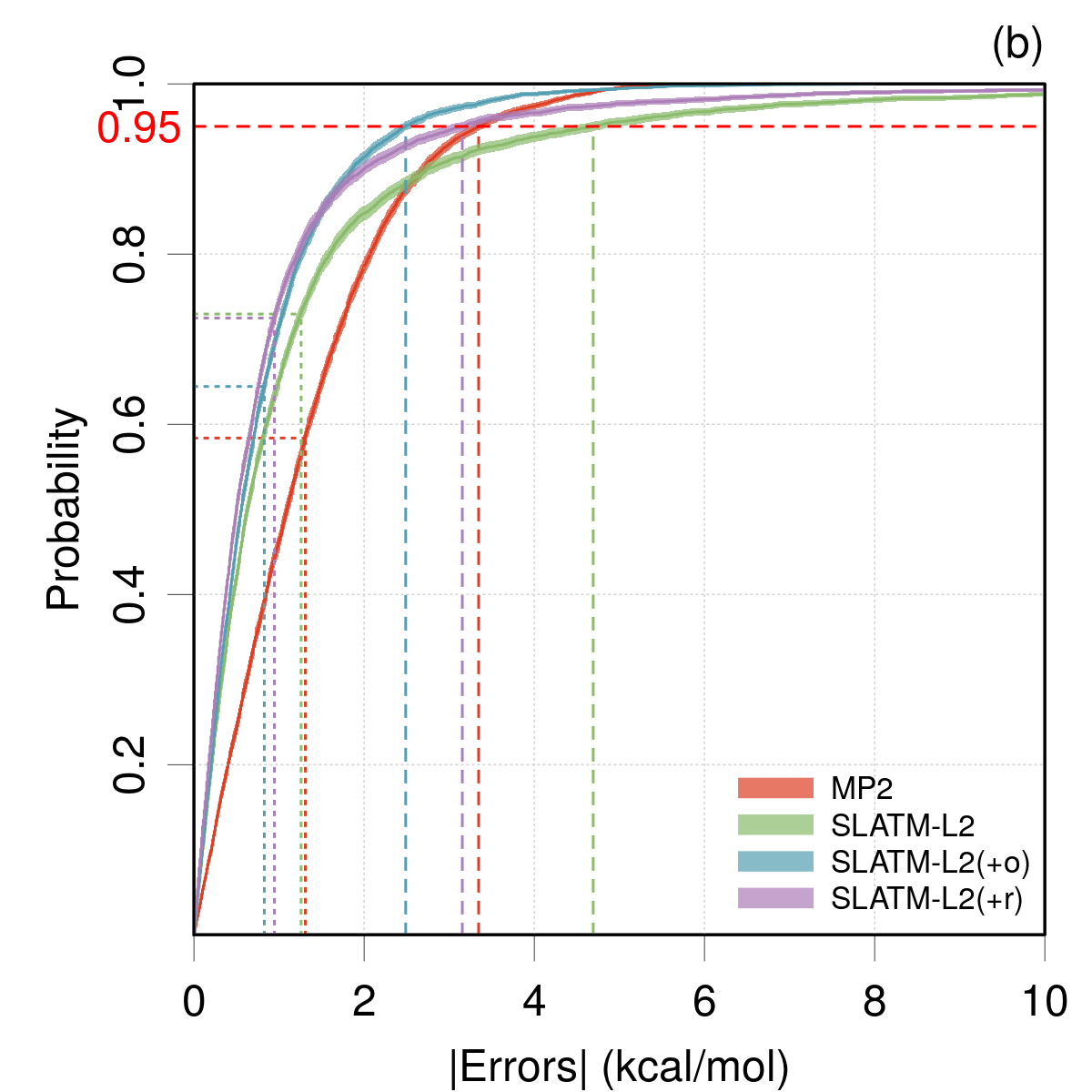
Figure 2: ECDFs of the absolute errors the effective atomization energies $E^{*}$ with respect to CCSD(T): (a) original methods; (b) comparison with SLATM-L2 trained on a learning set augmented with 350 systems (+o: outliers of SLATM-L2; +r: random systems). The dashed lines signal the $Q_{95}$ statistic for each set, and the dotted lines the corresponding MAE.

In order to substantiate the interpretation of the error statistics, it is important (1) to check that the error distributions are not dominated by systematic errors (trends), and (2) to assess their normality or lack thereof. This is essential if any quantification of the predictive ability of the methods is of interest.

Trends.

Plots of the error sets (Fig. 1(a-d)) show that the ML errors present weak (linear) trends, whereas HF and MP2 are more affected. For comparison of their performances, the data sets have been linearly corrected to remove the trends, according to Pernot et al.[1]. Summary statistics for corrected methods (with a ’lc-’ prefix) are reported in Table 1, showing a small impact on all statistics. The normality Shapiro-Wilk statistic is improved for HF and MP2, and the error distribution for lc-MP2 is practically normal. After linear correction, and considering the small uncertainty on the linear correction parameters due to the large size of the dataset, the prediction uncertainty can be estimated by the RMSD [1]. This enables to assess the better performance of MP2 in terms of prediction uncertainty.

Normality.

Comparison of the histograms with their gaussian fit in Fig. 1(a-d) shows clearly that the distributions for HF and MP2, albeit trended, are nearly normal. Note that this is not a general trend of quantum chemistry methods [2]. On the contrary, the error distribution for SLATM-L2 is notably non-normal, with a narrow central peak and wide tails. Because of the large number of points concentrated near the center, the tails of the distribution are not visible on the histogram in Fig. 1(d). They are much more apparent on the QQ-plot in Fig. 4(a), which will be introduced in Section 3.3.

ECDFs.

Considering Fig. 2, one see that the absolute errors ECDFs for SLATM-L2 and MP2 intersect around 3 kcal/mol. Below this value, SLATM-L2 presents smaller absolute errors, with the opposite above. It is clearly visible here why SLATM-L2 has a larger $Q_{95}$ than MP2. Indeed, one sees also on Figs. 1 (b,d) that SLATM-L2 has a non-negligible set of errors much larger than the largest MP2 errors. A similar effect occurs even between HF and SLATM-L2, the latter presenting larger absolute errors above approximately 8 kcal/mol.

Computational time aside, the choice between MP2 and SLATM-L2 as a predictor for CCSD(T) energies depends on the acceptance by the user of a small percentage of large errors. SLATM-L2 would largely benefit from a reduction of such large errors. In the following, we focus on the SLATM-L2 error set to identify underlying features linked to large prediction errors.

3.2 Chemical analysis

In order to get a chemical insight on the error trends in the present dataset, the absolute errors have been analyzed as functions of several compositional data, such as the number of individual species in the composition (H, C, N, O, S, Cl) and the Double Bond Equivalent (DBE), which estimates the degree of unsaturation (number of double bonds and rings) [27]

$$\mathrm{DBE}=n\mathrm{C}-\frac{n\mathrm{H}+n\mathrm{Cl}}{2}+\frac{n\mathrm{N}}{2}+1$$ (4)

where $n\mathrm{X}$ is the number of $\mathrm{X}$ atoms in the molecule. Note that in this formula divalent atoms do not contribute to the DBE.

Sensitivity of the errors to the various variables has been estimated by using rank correlation coefficients. The largest sensitivity has been found with respect to the number of hydrogen atoms in the molecule ($n\mathrm{H}$) and the DBE. Note that both indicators are not independent (DBE is anti-correlated with $n\mathrm{H}$), and that $n\mathrm{H}$ is strongly correlated with the number of atoms in the molecule.

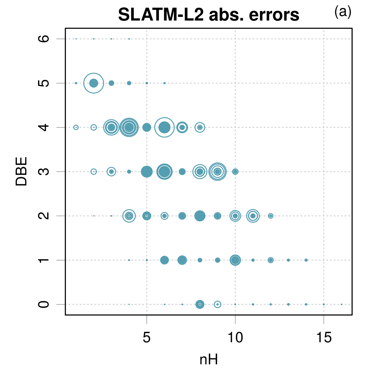
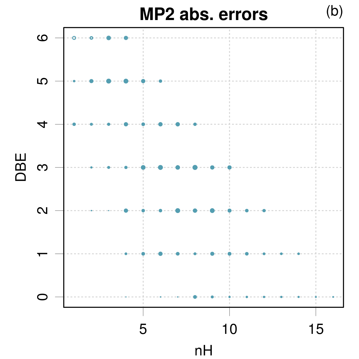
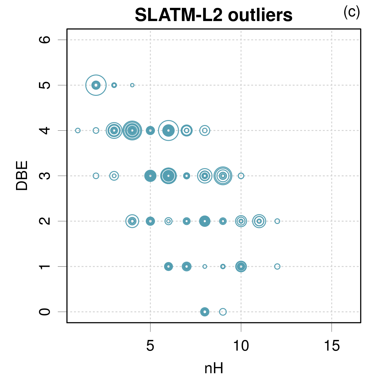
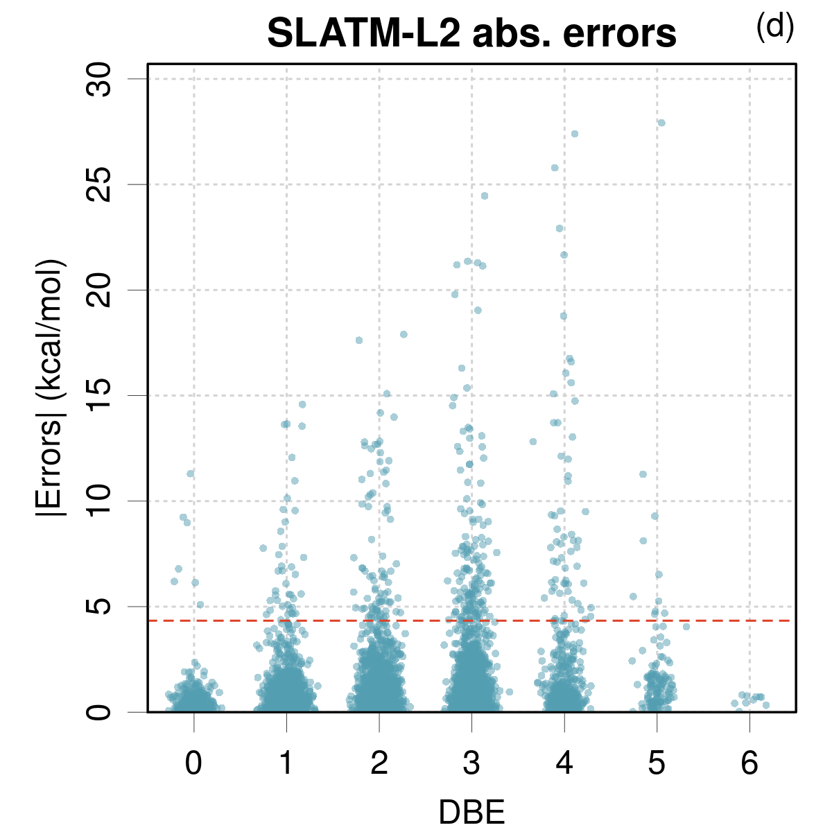
Figure 3: Error distributions of SLATM-L2 (a) and MP2 (b) and outliers of SLATM-L2 (c) as functions of the number of H atoms and Double Bond Equivalent (DBE) of the molecules. The circles diameters are on a common scale for all figures and are proportional to the absolute errors. The distribution of SLATM-L2 errors for each DBE class is shown in (d), where the horizontal dashed line represents the $5*\sigma_{1}$ selection threshold for outliers.

The distribution of the absolute errors sorted by DBE class is shown in Fig. 3(d). Distributions of the absolute errors according to $n\mathrm{H}$ and DBE are presented in (Fig. 3(a,b)), where each datum is represented by a circle of diameter proportional to its absolute error. The scale is identical for all the series of plots. The imprint of the points cloud reflects the correlation between $n\mathrm{H}$ and DBE.

For SLATM-L2, some systems with DBE = 3-5 present very large errors, and the maximal absolute error increases almost linearly from DBE = 0 to 4. All compositions with DBE = 6 are correctly predicted, although, except for C5H2N2, none of those compositions are found in the learning set. For molecules with DBE = 0, all heavy atoms are sp³-hybridized, being the most local and thus transferable and easy to learn by QML models. For molecules with DBE = 6, bond environments are non-local, but could be easily covered by the training set. Therefore, low prediction errors are expected in these cases.

For MP2, the points cloud in Fig. 3(b) presents no strong feature, but the errors seem smaller for DBE = 0, and for each DBE class, there seems to be a maximum around the mid-range of admissible $n\mathrm{H}$ values.

3.3 Outliers analysis

The non-normality of the errors distribution for SLATM-L2 is clearly visible on the QQ-plot in Fig. 4(a). There is a near linear section at the center if the distribution, seen by comparison with the interquartile line, and also linear sections in the tails of the distribution. The core of the distribution is therefore dominated by a normal component, as well as the tails, albeit with different widths (and centers). Indeed, a bi-normal fit (Eq. 3) provides a good representation of the distribution. Note that to get a perfect fit, as much as four components are needed, but the bi-normal representation is sufficient for the present purpose of outliers analysis.

The graphical results and optimal parameters are reported in Fig. 4(b). This decomposition provides a strong component (weight 0.83) with a sub-kcal/mol standard deviation ($\sigma_{1}=0.87$ kcal/mol), and a weaker component (weight: 0.17) with a much larger dispersion ($\sigma_{2}=5.5$ kcal/mol). Both components are nearly zero-centered.

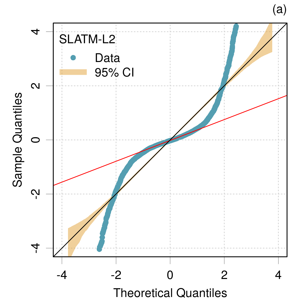
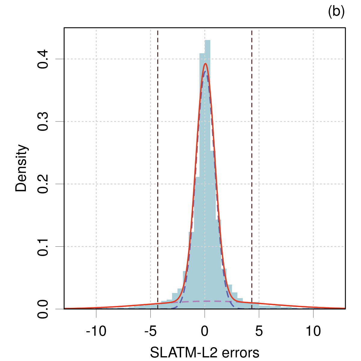
	Parameters of the bi-normal fit $i$ $\mu_{i}$ (kcal/mol) $\sigma_{i}$ (kcal/mol) $w_{i}$ 1 -0.06 0.87 0.83 2 -0.47 5.50 0.17

Figure 4: Non-normality of the SLATM-L2 errors distribution. (a) Normal QQ-plot: the orange area depicts the Monte Carlo estimated statistical variability for a normal sample of the same size; the red line passes through the first and third quartiles of the sample. (b) Optimal bi-normal density superimposed on errors histogram: the dashed vertical lines delimit the $5*\sigma_{1}$ threshold for outliers identification.

Composition	DBE	medAE	maxAE	nOutl/nTest	nLearn
C4H2N2O	5	10.28	27.92	4/12	3
C5H6N2	4	6.28	27.40	10/60	17
C4H4N2O	4	8.13	25.79	14/64	13
C6H9N	3	9.14	24.46	9/152	25
C4H3NO2	4	10.93	21.66	4/25	3
C4H6N2O	3	6.22	21.36	37/223	39
C5H6O2	3	6.07	21.29	11/115	22
C6H8O	3	6.02	19.79	10/203	33
C6H11N	2	12.71	17.90	6/207	29
C3H4O3S	2	9.86	17.62	5/6	1
C4H3NOS	4	13.13	16.76	2/6	2
C5H4OS	4	16.60	16.60	1/3	0
C4H5NO2	3	8.44	15.36	20/109	18
C6H10O	2	5.32	15.09	4/242	51
C6H7N	4	9.48	15.08	6/51	6
C4H6N2S	3	6.71	14.91	14/40	8
C4H10N2S	1	13.63	14.58	5/5	0
C4H8N2S	2	12.10	14.18	12/12	0
C7H8	4	9.98	13.71	2/43	7
C6H6O	4	8.67	13.71	5/66	6
C3H7N1O2S	1	6.88	12.07	9/15	1
C3H3NO2S	3	8.57	12.04	2/2	1
C6H6	4	11.99	11.99	1/5	5
C5H8O2	2	5.72	11.87	6/229	26
C3H5NO2S	2	7.39	11.31	5/5	2
C3H8O3S	0	6.49	11.30	6/8	0
C5H5NO	4	6.08	11.20	7/83	10
C3H6O3S	1	7.77	10.96	9/14	4
C5H10N2	2	5.21	10.83	4/194	28
C4H8N2O	2	5.66	10.20	20/245	50
C4H10N2O	1	5.56	10.14	9/151	25

Table 2: Composition of the 5$\sigma$ outliers with maximum absolute error above 10 kcal/mol. For each composition, one defines medAE: median Absolute error in outlier isomers; maxAE: max Absolute error in outlier isomers; nOutl: number of isomers in the outlier set; nTest: number of isomers in the test set; nLearn: number of isomers in the learning set.

In order to identify the systems involved in the widest contribution, one selects outliers with respect to the most concentrated component, i.e. points lying at more than $5*\sigma_{1}$ from the center of the concentrated component ($\mu_{1}$).

This filter selects 350 molecules (about 6 % of the test set population). The chemical formulae of these systems are analyzed in terms of $n\mathrm{H}$ and DBE (Fig. 3(c)). Systems with DBE = 0 or 6 are practically absent from the list of outliers (at the exception of a few DBE = 0 ones). The outliers with the largest absolute errors are molecules with some unsaturation (DBE $\geq$ 3).

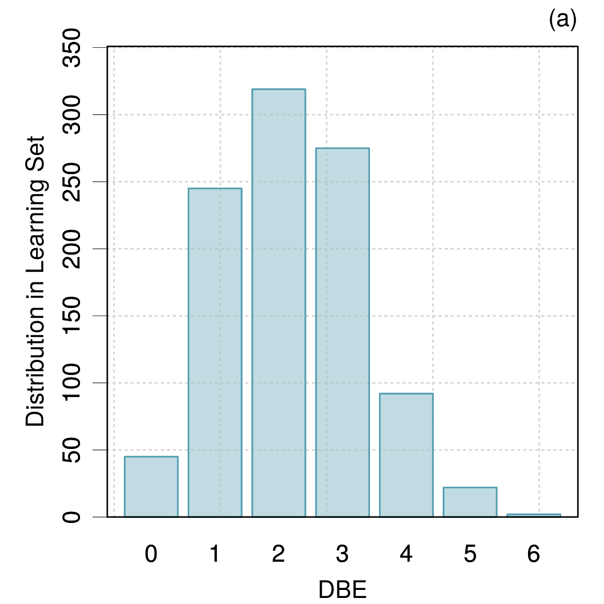
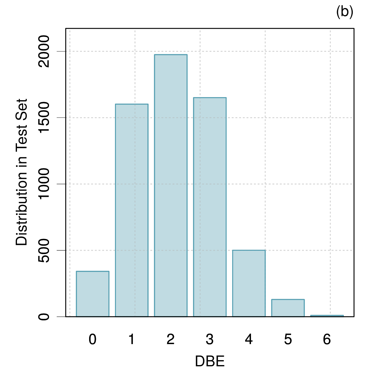
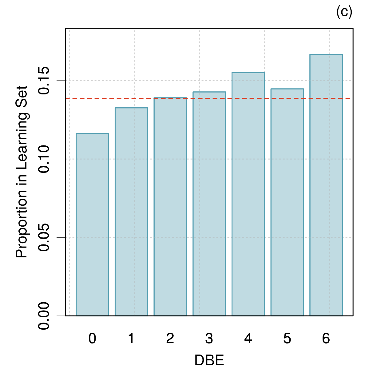
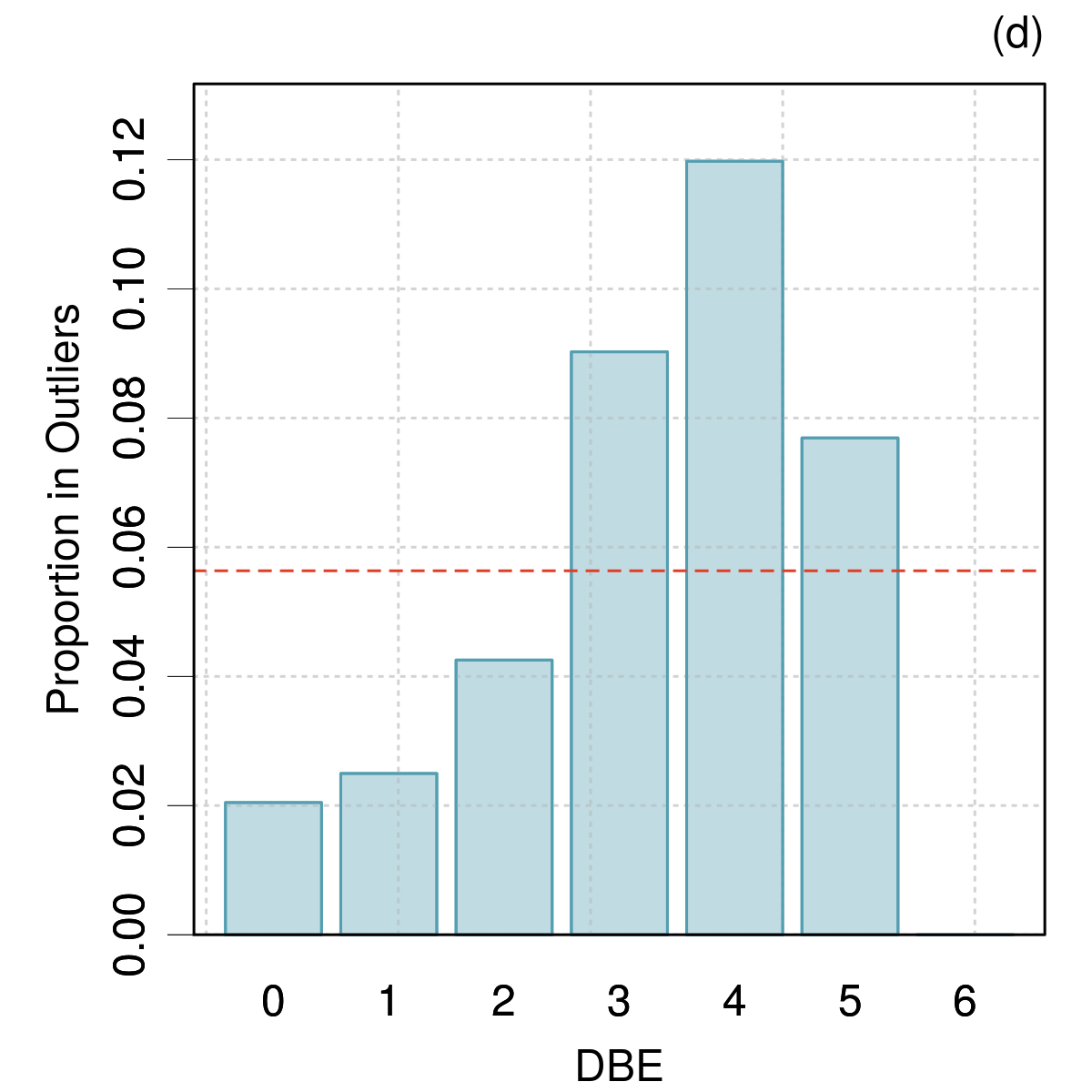
Figure 5: DBE distribution in (a) the learning set and (b) the test set; (c) proportion of each DBE class in the learning set with respect to the distribution in the full data set (learning + test); (d) proportion of SLATM-L2 outliers in each DBE class with respect to the distribution in the test set. The horizontal dashed lines represent the mean proportion over the reference dataset.

Fig. 5 reports the DBE distributions in the leaning set Fig. 5(a) and test set Fig. 5(b). In both cases, the distributions are peaked around DBE=2. The distributions are similar because the learning set is a random selection in the full dataset. The ratio of the learning set DBE distribution over the full dataset DBE distribution is practically constant, with slight increasing trend that might be a random effect (Fig. 5(c)). In contrast, Fig. 5(d) shows that the DBE classes around DBE=4 contain a larger proportion of outliers than the lower DBE classes, up to 12 % for DBE = 4. Outliers are not uniformly distributed amongst the DBE classes.

Compositions with a maximum absolute error larger than 10 kcal/mol are listed in Table 2. The composition with the largest absolute error is C4H2N2O (27.9 kcal/mol for the molecule SMILES:C#CC(=N#N)C=O [28]). This molecule, with DBE=5, has 3 isomers/configurations in the learning set and 12 in the test set, 4 of which are outliers. The second one is C5H6N2 (27.4 kcal/mol, SMILES:c1cnn2c1CC2), with 17 configurations in the learning set, 60 in the test set, 10 of which are outliers.

One can see in this list that most outliers compositions present some isomers in the learning set. Unsurprisingly, it contains also a few compositions absent from the learning set, e.g., C5H4OS (SMILES:c1c2c(cs1)OC2), but as seen above for the DBE=6 compounds, this is not systematically associated with poor predictions.

The impact on the error statistics of the removal of the 350 outliers from the test set is reported in Table 1, as method SLATM-L2(-o). The improvement is noticeable on all aspects: better normality of the distribution, reduced bias (MSE $\simeq 0$), and a notable reduction, as expected, of MAE, RMSD and $Q_{95}$.

3.4 Expanding the learning set with outliers

Having identified 350 systems for which SLATM-L2 provides exceedingly large errors, we want to check if their transfer to the learning set has a positive impact on prediction performances. To validate the impact of this learning set augmentation, a list of 350 systems has been transferred from the test set to the learning set according to two selections: (1) the outliers identified above (SLATM-L2(+o)), and (2) a random choice (SLATM-L2(+r)), both resulting in a learning set of size 1350. The second scenario is a control to assess the size effect of the learning set. Note that the present random selection contains 22 of the 350 outliers ($\simeq$ 6 %), in proportion with the random selection of 350 points among 6211.

The SLATM-L2 model has been retrained with both learning sets, and the error distribution analysis has been performed for these two new datasets. The results are reported in Table 1 and Fig. 1(e,f), 2(b), Fig. 6.

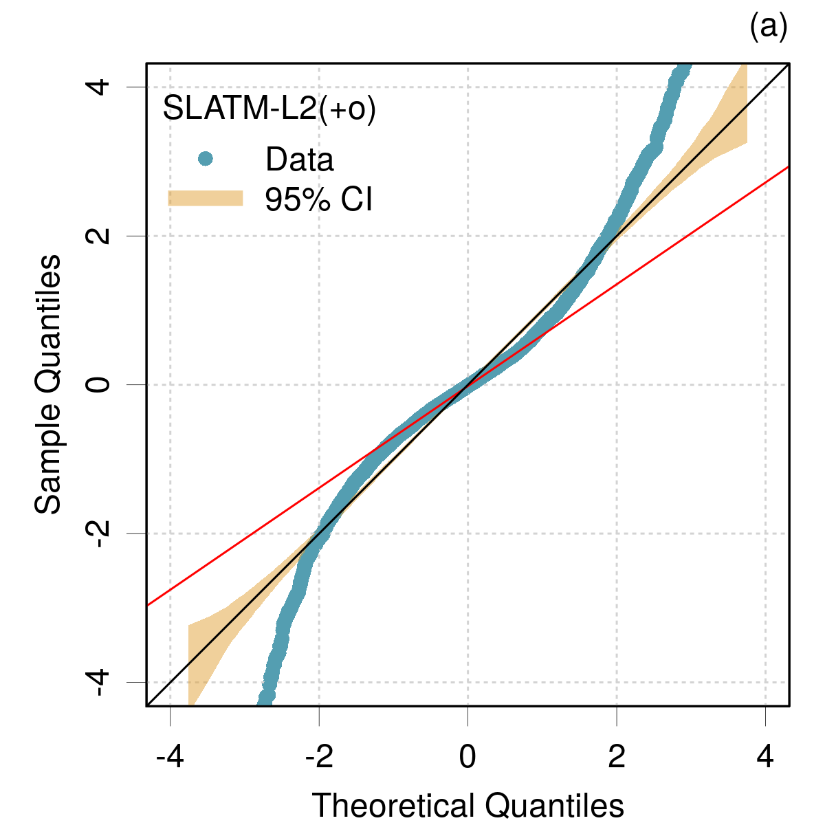
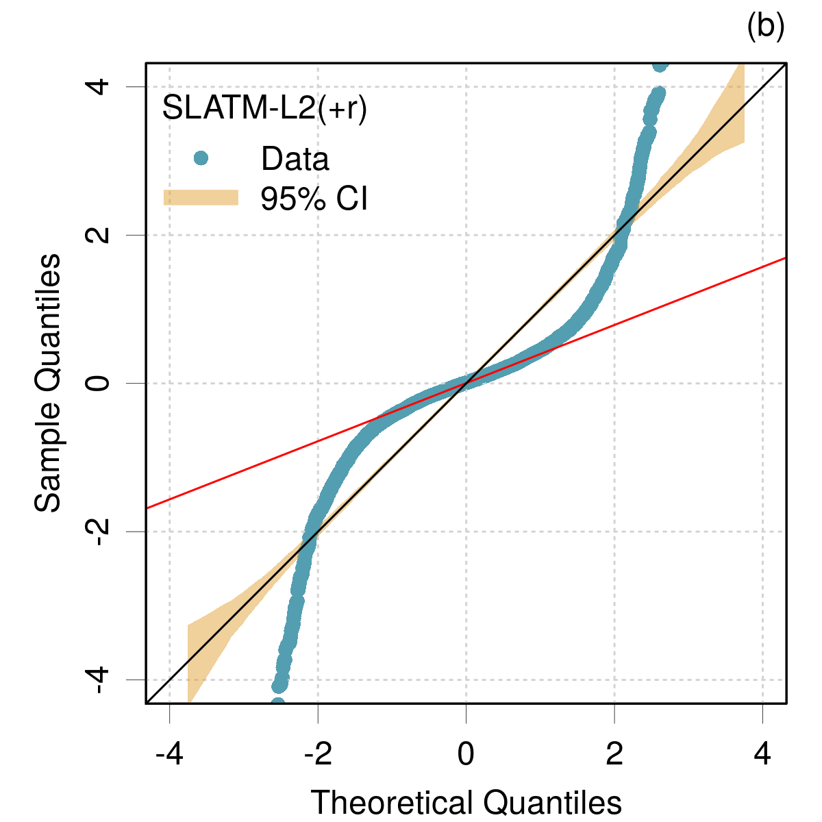
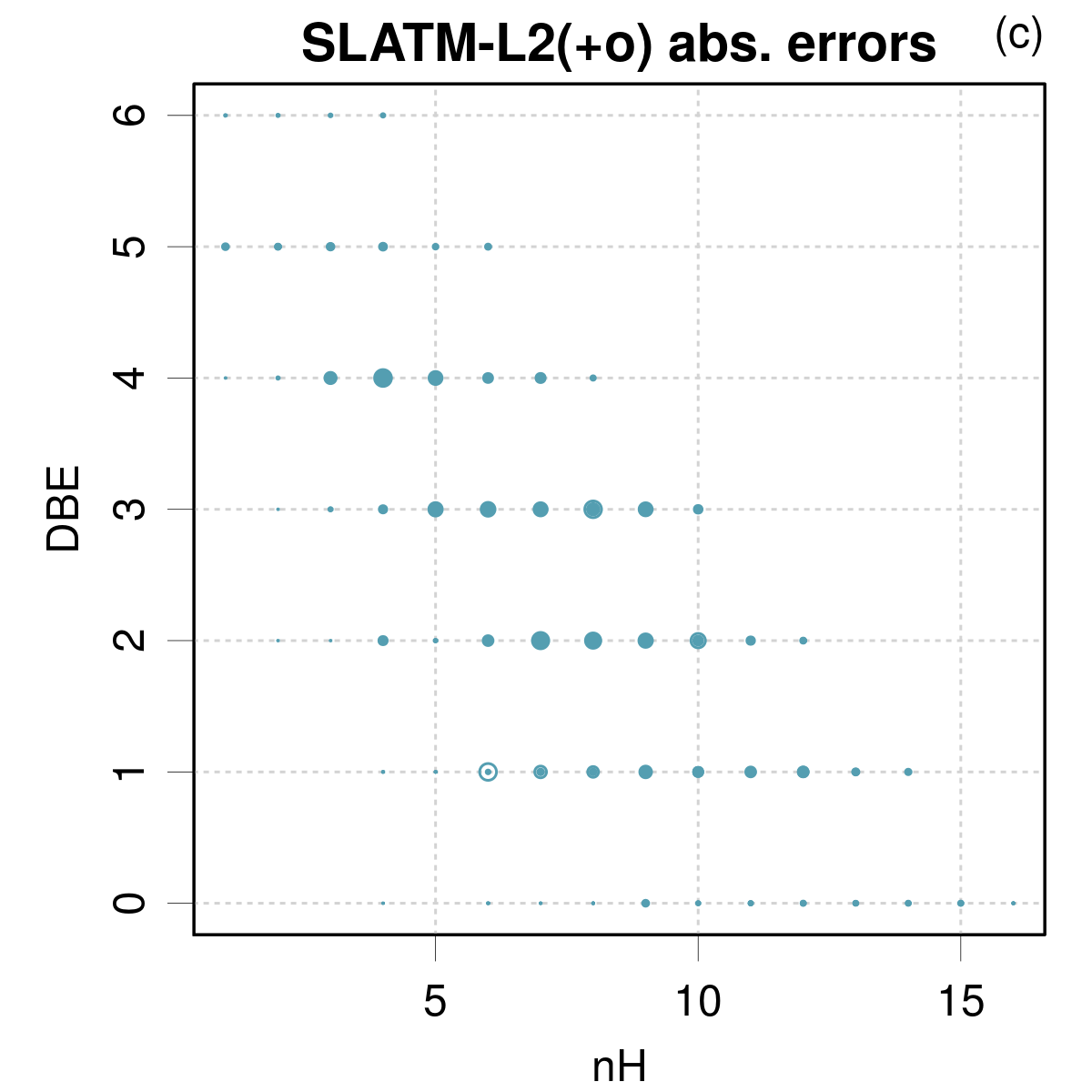
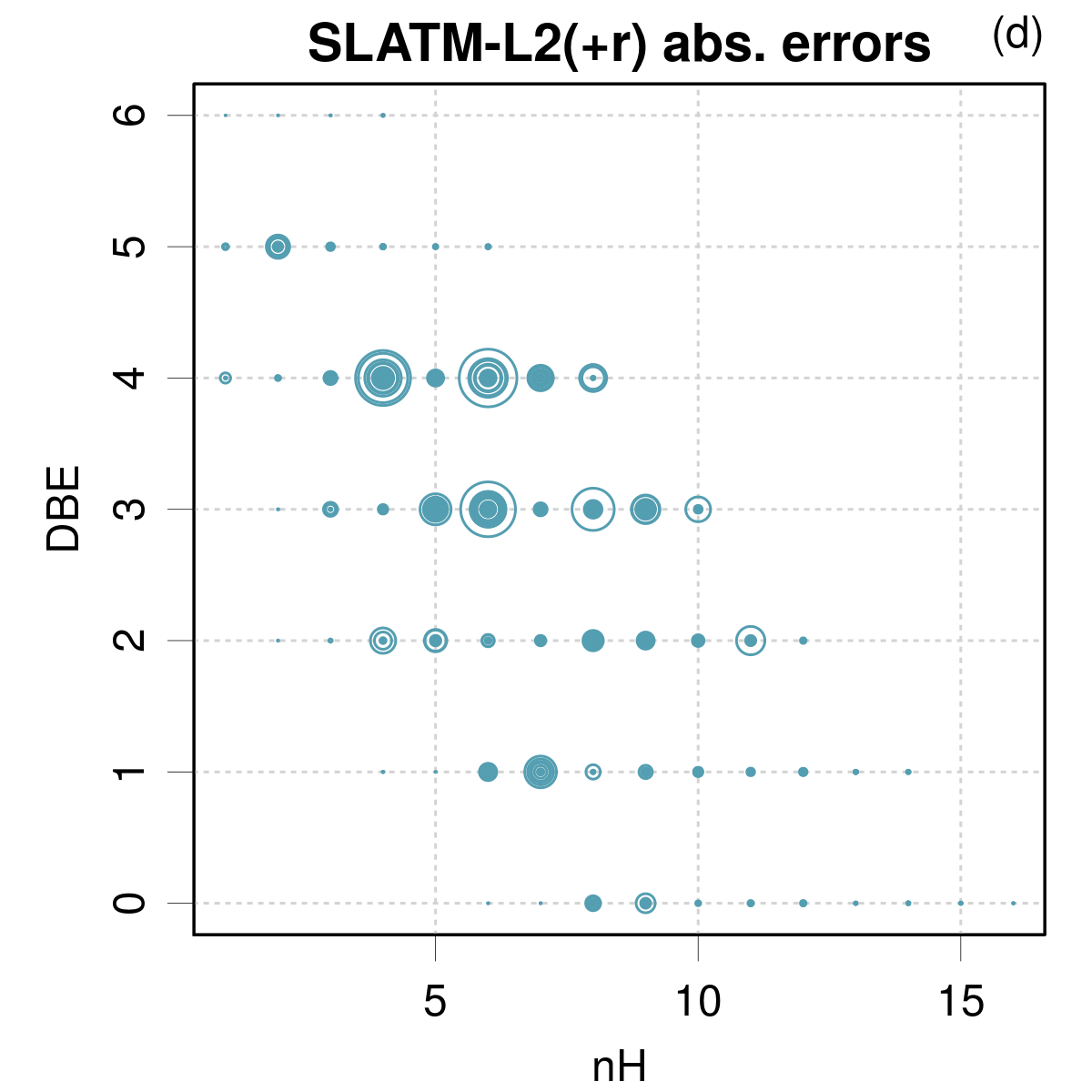
Figure 6: Normal QQ-plots of the error distributions for (a) SLATM-L2(+o) and (b) SLATM-L2(+r) (see Fig. 4 for details); (c,d): absolute error distributions as functions of the number of H atoms and Double Bond Equivalent (DBE) of the molecules. The circles diameters are on a common scale for all figures and are proportional to the absolute errors.

A first aspect to consider is how the inclusion of the outliers in the learning set (SLATM-L2(+o)) affects the prediction errors with respect to the pruned error set (SLATM-L2(-o)) presented in the previous section. Globally, the improvement is minor, but consistent. The MSE and RMSD are identical, the MAE is barely decreased, and the $Q_{95}$ is slightly improved from 2.70 to 2.49 kcal/mol. The learning on the outliers has been transferred to some of the predictions.

Then, we compare the gain in prediction quality due to the augmentation of the learning set by outliers versus random systems. The MAE values of SLATM-L2(+o): 0.83 and SLATM-L2(+r): 0.95 kcal/mol indicate a statistically significant, but rather weak effect of the outliers selection, whereas the sheer augmentation of the learning set size improves notably the MAE of the original method by 0.3 kcal/mol. The MSE shows that the slight bias of the original SLATM-L2 has been essentially corrected in both cases. Impact on the RMSD is larger than on the MAE (1.20 for ’+o’ vs. 1.89 kcal/mol for ’+r’), with a notable reduction of 1.24 kcal/mol from the initial RMSD. Similarly, the decrease in $Q_{95}$ is important for SLATM-L2(+o), from 4.7 to 2.49 kcal/mol, and much less for SLATM-L2(+r), to 3.15 kcal/mol, which reaches the level of MP2 (3.34 kcal/mol). One sees also that the normality of the distribution has been improved for SLATM-L2(+o) (Kurt from 29 to 8.1; $W$ from 0.71 to 0.935), which is not the case for the random selection (Kurt =46; $W$ = 0.66).

Without looking at the plots of the distributions, this set of statistics points to a notable improvement of the error distribution on all criteria for the outliers-augmented learning set. By contrast, the improvement by random selection of the 350 systems, although significant, does not improve the quality of the error distribution, which stays strongly leptokurtic. This can be appreciated on the QQ-plots for both error distributions in Fig. 6(a,b).

The ECDFs of the error distributions illustrate clearly the analysis of the summary statistics (Fig. 2(b)). The augmented SLATM-L2 versions have more concentrated absolute errors than SLATM-L2. In the case of SLATM-L2(+o) the large errors have essentially vanished and the overall performance is better than SLATM-L2 and even than MP2. Albeit SLATM-L2(+r) is also more concentrated, it still presents a set of systems with large errors, exceeding those of MP2. The comparison of the $n\mathrm{H}$/DBE plots in Fig. 6(c,d) and depicts precisely this point.

4 Discussion

We analyzed the prediction error distribution of a ML method (KRR-SLATM-L2) for effective atomization energies of QM7b molecules calculated at the level of theory CCSD(T)/cc-pVDZ. Error distributions of standard computational chemistry methods (HF and MP2) at the same basis set level and for the same reference dataset were also estimated for comparison.

We have shown that the shapes of error distributions should carefully be considered when one attempts to quantify the prediction performance of a method. MAE-based benchmarks neglect crucial information, that is better rendered by probabilistic estimators such as $Q_{95}$. Similar values of the MAE might hide very different error distributions, with a strong impact on the assessment and ranking of methods. In particular, ML prediction error distributions can be strongly non-normal, notably leptokurtic, which poses a problem of prediction reliability, as they might have a non-negligible probability to produce very large errors. Identification of systems with large prediction errors and their inclusion into the learning set improves significantly the prediction error distribution. These main points are further discussed below.

4.1 Limitations of the present study

The QM7b dataset has a nice feature of diversity, albeit it is small in total size. A natural yet undesired consequence is that the dataset is highly inhomogeneous in chemical space, the conclusions drawn above from the results on QM7b may therefore not be extensible to other datasets, such as QM9 [29, 30] (less diverse in composition, yet larger in total set size). Considering these properties of QM9, one might expect the prediction error distribution for SLATM-L2 to be less leptokurtic than for QM7b, and a less problematic use of MAE for performance assesment. This has however to be checked, but at the moment, one has no access to hierarchical properties for the full QM9, as for QM7b.

In this paper we assessed the prediction of energy, which is extensive in nature. There exists a set of intensive properties as well and which are typically difficult to learn. The generalizability of our observations to these properties should also be confirmed in future studies.

4.2 Analysis of the SLATM-L2 error distribution

A major feature of the SLATM-L2 error distribution is the presence of a strong peak of small errors and wide tails of large errors. This leptokurtic distribution has been successfully modeled as a mixture of two normal distributions, both practically centered on zero, with standard deviations 0.87 and 5.5 kcal/mol and a mixture ratio 83:17. Based on this analysis, we explore the chemical identity of the systems with large errors.

It is not possible to unscramble both populations in the area where the most concentrated population is dominant, but if one goes far enough in the tails (beyond 5 times 0.87 kcal/mol) one finds a large majority of systems belonging to the population with large errors. Such 350 systems were identified and tagged as outliers. A chemical analysis of these systems based on their DBE revealed that compositions with high levels of unsaturation (DBE$=3-5$) are overrepresented with respect to their abundance in the test set. It seems therefore that the large prediction errors are not randomly distributed over the QM7b molecules, which might provide insights for improved molecular descriptors or a better design of the learning set.

In fact, if the learning set is augmented with these outliers (SLATM-L2(+o)), one gets better prediction performances than if one augments the learning set with 350 randomly chosen systems (SLATM-L2(+r)). This suggests an iterative method for the design of learning sets that might deserve further consideration.

4.3 Importance for ML to aim at near-normality of error distributions

For ML methods to be used trustfully as replacements of quantum chemistry methods, one needs to have a reliable measure of their accuracy. Ideally, this should be quantified by a single number characterizing the predictive ability of a method. This requires a finite variance, homogeneous, error distribution (with a dispersion that does not vary strongly within the calculated property range) and a zero-centered symmetric error distribution. Moreover, we have seen that leptokurtic error distributions with a strong core of small errors and tails of large errors, as described above by a bi-normal distribution might not be properly summarized by a single dispersion statistic. The MAE is not a good choice in such cases, and $Q_{95}$ presents a more reliable alternative, which quantifies the risk of large prediction errors, even in the case of non-zero-centered symmetric error distributions.

We have shown that inclusion of outliers in the learning set of the SLATM-L2 method could result in a notable improvement of the shape of its prediction errors distribution. One might also presume that the use of much larger learning sets should improve the structure of the prediction error distribution.

4.4 What probability does one have to reach the chemical accuracy ?

Whatever the pertinence of this question, it cannot be answered by considering the MAE, contrary to a still too common practice in the benchmarking literature to use it as an “accuracy” measure. The example of the SLATM-L2(+o) method shows that a sub-chemical-accuracy MAE (0.86 kcal/mol) can hide a non-negligible risk (about 30 %) to exceed this limit.

A direct answer to the question is provided by the ECDF of the errors and $C(\eta)$ with $\eta=$1 kcal/mol. The values reported in Table 1 tell us that none of the studied methods achieves the 1 kcal/mol threshold with a high probability. The best performers would be SLATM-L2 methods with augmented learning sets, with $C(1)=0.743$ for the (+r) version. Even in this case, one has no firm guarantee to reach chemical accuracy for any new prediction, the risk being higher than 25 % to overpass the threshold. Note that this is a notable improvement over MP2, for which the risk is about 55 %. Besides, this qualifies chemical accuracy with respect to CCSD(T), not with respect to experimental values.

4.5 On the use of statistics to rank methods

In Section 3.1, we outlined that the basic summary statistics (MAE, RMSD) provided contradictory information about the SLATM-L2 prediction performances, notably when compared to MP2. SLATM-L2 has a smaller slightly smaller MAE than MP2 (1.26 vs. 1.31 kcal/mol) but a much larger RMSD (2.44 vs. 1.67). This is a consequence of the peculiar shape of the error distribution for SLATM-L2. In line with the RMSD values, MP2 achieves a notably smaller $Q_{95}$ value (3.34 vs. 4.7 kcal/mol), meaning that SLATM-L2 is susceptible of larger errors than MP2.

Given this set of information and computation time aside, one would most certainly pick MP2 over SLATM-L2 as a reasonable predictor of CCSD(T) energies, with a prediction uncertainty of approximately 1.7 kcal/mol for $E^{*}$ (RMSD in Table 1), and with added confidence from the near-normality of the distribution, reducing the risk of rogue predictions that might be expected from SLATM-L2. Finally, the modified SLATM-L2(+o) method, for which the learning set was augmented with SLATM-L2 outliers, clearly outperforms both SLATM-L2 and MP2 for all statistics.

This illustrates once more that the MAE is not sensitive to major differences in the shape of the errors distributions, as was shown by Pernot and Savin [2]: even for normal distributions, many combinations of MSE and RMSD can produce the same MAE. The case is even worse for non-normal distributions, where the MAE loses its ability to quantify prediction uncertainty. It is clear that the MAE should not be used as a unique scoring statistic, and that it should at least be complemented (or replaced) by probabilistic indicators such as $Q_{95}$ .

References

- [1] P. Pernot, B. Civalleri, D. Presti, and A. Savin. Prediction uncertainty of density functional approximations for properties of crystals with cubic symmetry. J. Phys. Chem. A, 119:5288–5304, 2015. doi:10.1021/jp509980w.
- [2] P. Pernot and A. Savin. Probabilistic performance estimators for computational chemistry methods: the empirical cumulative distribution function of absolute errors. J. Chem. Phys., 148:241707, 2018. doi:10.1063/1.5016248.
- [3] J. P. Perdew, J. Sun, A. J. Garza, and G. E. Scuseria. Intensive atomization energy: Re-thinking a metric for electronic structure theory methods. Z. Phys. Chem., 230:737–742, 2016. doi:10.1515/zpch-2015-0713.
- [4] K. Lejaeghere, L. Vanduyfhuys, T. Verstraelen, V. V. Speybroeck, and S. Cottenier. Is the error on first-principles volume predictions absolute or relative? Comput. Mater. Sci., 117:390–396, 2016. doi:10.1016/j.commatsci.2016.01.039.
- [5] F. A. Faber, L. Hutchison, B. Huang, J. Gilmer, S. S. Schoenholz, G. E. Dahl, O. Vinyals, S. Kearnes, P. F. Riley, and O. A. von Lilienfeld. Prediction errors of molecular machine learning models lower than hybrid DFT error. J. Chem. Theory Comput., 13:5255–5264, 2017. doi:10.1021/acs.jctc.7b00577.
- [6] P. Zaspel, B. Huang, H. Harbrecht, and O. A. von Lilienfeld. Boosting quantum machine learning models with a multilevel combination technique: Pople diagrams revisited. J. Chem. Theory Comput., 15(3):1546–1559, 2019. doi:10.1021/acs.jctc.8b00832.
- [7] P. Pernot and A. Savin. Probabilistic performance estimators for computational chemistry methods: Systematic improvement probability and ranking probability matrix. II. Applications. J. Chem. Phys., 152:164109, 2020. doi:10.1063/5.0006204.
- [8] N. Mohd Razali and B. Yap. Power Comparisons of Shapiro-Wilk, Kolmogorov-Smirnov, Lilliefors and Anderson-Darling Tests. J. Stat. Model. Analytics, 2:21–33, 01 2011. URL: https://pdfs.semanticscholar.org/dcdc/0a0be7d65257c4e6a9117f69e246fb227423.pdf.
- [9] K. Klauenberg and C. Elster. Testing normality. tm - Technisches Messen, 86:773–783, 2019. doi:10.1515/teme-2019-0148.
- [10] B. Ruscic. Uncertainty quantification in thermochemistry, benchmarking electronic structure computations, and active thermochemical tables. Int. J. Quantum Chem., 114:1097–1101, 2014. doi:10.1002/qua.24605.
- [11] A. J. Thakkar and T. Wu. How well do static electronic dipole polarizabilities from gas-phase experiments compare with density functional and MP2 computations? J. Chem. Phys., 143:144302, 2015. doi:10.1063/1.4932594.
- [12] A. P. Scott and L. Radom. Harmonic Vibrational Frequencies: An Evaluation of Hartree-Fock, Möller-Plesset, Quadratic Configuration Interaction, Density Functional Theory, and Semiempirical Scale Factors. J. Phys. Chem., 100(41):16502–16513, 1996. doi:10.1021/jp960976r.
- [13] P. Pernot and F. Cailliez. Comment on "Uncertainties in scaling factors for ab initio vibrational zero-point energies" [J. Chem. Phys. 130, 114102 (2009)] and "Calibration sets and the accuracy of vibrational scaling factors: A case study with the X3LYP hybrid functional" [J. Chem. Phys. 133, 114109 (2010)]. J. Chem. Phys., 134:167101, 2011. doi:10.1063/1.3581022.
- [14] K. Lejaeghere, J. Jaeken, V. V. Speybroeck, and S. Cottenier. Ab initio based thermal property predictions at a low cost: An error analysis. Phys. Rev. B, 89:014304, jan 2014. doi:10.1103/physrevb.89.014304.
- [15] K. Lejaeghere, V. Van Speybroeck, G. Van Oost, and S. Cottenier. Error estimates for solid-state density-functional theory predictions: An overview by means of the ground-state elemental crystals. Crit. Rev. Solid State Mater. Sci., 39:1–24, 2014. doi:10.1080/10408436.2013.772503.
- [16] J. Proppe and M. Reiher. Reliable estimation of prediction uncertainty for physicochemical property models. J. Chem. Theory Comput., 13:3297–3317, 2017. doi:10.1021/acs.jctc.7b00235.
- [17] R. Ramakrishnan, P. O. Dral, M. Rupp, and O. A. von Lilienfeld. Big data meets quantum chemistry approximations: The -machine learning approach. J. Chem. Theory Comput., 11:2087–2096, 2015. doi:10.1021/acs.jctc.5b00099.
- [18] L. Ward, B. Blaiszik, I. Foster, R. S. Assary, B. Narayanan, and L. Curtiss. Machine Learning Prediction of Accurate Atomization Energies of Organic Molecules from Low-Fidelity Quantum Chemical Calculations. MRS Commun., 9:891–899, 2019. doi:10.1557/mrc.2019.107.
- [19] J. Proppe, S. Gugler, and M. Reiher. Gaussian Process-Based Refinement of Dispersion Corrections. J. Chem. Theory Comput., 15:6046–6060, Jun 2019. doi:10.1021/acs.jctc.9b00627.
- [20] R Core Team. R: A Language and Environment for Statistical Computing. R Foundation for Statistical Computing, Vienna, Austria, 2019. Version 3.6.1. URL: https://www.R-project.org/.
- [21] A. Canty and B. Ripley. boot: Bootstrap Functions (Originally by Angelo Canty for S), 2019. R package version 1.3-22. URL: https://CRAN.R-project.org/package=boot.
- [22] L. Komsta and F. Novomestky. moments: Moments, cumulants, skewness, kurtosis and related tests, 2015. R package version 0.14. URL: https://CRAN.R-project.org/package=moments.
- [23] D. Young, T. Benaglia, D. Chauveau, and D. Hunter. mixtools: Tools for Analyzing Finite Mixture Models, 2020. R package version 1.2.0. URL: https://CRAN.R-project.org/package=mixtools.
- [24] T. Benaglia, D. Chauveau, D. R. Hunter, and D. Young. mixtools: An R package for analyzing finite mixture models. J. Stat. Softw, 32:1–29, 2009. doi:10.18637/jss.v032.i06.
- [25] G. Montavon, M. Rupp, V. Gobre, A. Vazquez-Mayagoitia, K. Hansen, A. Tkatchenko, K.-R. Müller, and O. Anatole von Lilienfeld. Machine learning of molecular electronic properties in chemical compound space. New J. Phys., 15:095003, 2013. doi:10.1088/1367-2630/15/9/095003.
- [26] P. Pernot and A. Savin. Probabilistic performance estimators for computational chemistry methods: Systematic improvement probability and ranking probability matrix. I. Theory. J. Chem. Phys., 152:164108, 2020. doi:10.1063/5.0006202.
- [27] V. Pellegrin. Molecular formulas of organic compounds: the nitrogen rule and degree of unsaturation. J. Chem. Educ., 60:626, 1983. doi:10.1021/ed060p626.
- [28] D. Weininger. Smiles, a chemical language and information system. 1. introduction to methodology and encoding rules. J. Chem. Inf. Comput. Sci., 28:31–36, 1988. doi:10.1021/ci00057a005.
- [29] L. Ruddigkeit, R. van Deursen, L. C. Blum, and J.-L. Reymond. Enumeration of 166 billion organic small molecules in the chemical universe database gdb-17. J. Chem. Inf. Model., 52:2864–2875, 2012. doi:10.1021/ci300415d.
- [30] R. Ramakrishnan, P. O. Dral, M. Rupp, and O. A. von Lilienfeld. Quantum chemistry structures and properties of 134 kilo molecules. Scientific Data, 1:140022, 2014. doi:10.1038/sdata.2014.22.