Applying Cyclical Learning Rate to Neural Machine Translation

Abstract

In training deep learning networks, the optimizer and related learning rate are often used without much thought or with minimal tuning, even though it is crucial in ensuring a fast convergence to a good quality minimum of the loss function that can also generalize well on the test dataset. Drawing inspiration from the successful application of cyclical learning rate policy for computer vision related convolutional networks and datasets, we explore how cyclical learning rate can be applied to train transformer-based neural networks for neural machine translation. From our carefully designed experiments, we show that the choice of optimizers and the associated cyclical learning rate policy can have a significant impact on the performance. In addition, we establish guidelines when applying cyclical learning rates to neural machine translation tasks. Thus with our work, we hope to raise awareness of the importance of selecting the right optimizers and the accompanying learning rate policy, at the same time, encourage further research into easy-to-use learning rate policies.

1 Introduction

There has been many interests in deep learning optimizer research recently (Reddi et al., 2018; Luo et al., 2019; Zhang et al., 2019; Liu et al., 2019). These works attempt to answer the question: what is the best step size to use in each step of the gradient descent? With the first order gradient descent being the de facto standard in deep learning optimization, the question of the optimal step size or learning rate in each step of the gradient descent arises naturally. The difficulty in choosing a good learning rate can be better understood by considering the two extremes: 1) when the learning rate is too small, training takes a long time; 2) while overly large learning rate causes training to diverge instead of converging to a satisfactory solution.

The two main classes of optimizers commonly used in deep learning are the momentum based Stochastic Gradient Descent (SGD) (Bottou, 2010) and adaptive momentum based methods (Duchi et al., 2010; Kingma and Ba, 2014; Reddi et al., 2018; Luo et al., 2019; Liu et al., 2019). The difference between the two lies in how the newly computed gradient is updated. In SGD with momentum, the new gradient is updated as a convex combination of the current gradient and the exponentially averaged previous gradients. For the adaptive case, the current gradient is further weighted by a term involving the sum of squares of the previous gradients. For a more detailed description and convergence analysis, please refer to Reddi et al. (2018).

In Adam (Kingma and Ba, 2014), the experiments conducted on the MNIST and CIFAR10 dataset showed that Adam has the fastest convergence property, compared to other optimizers, in particular SGD with Nesterov momentum. Adam has been popular with the deep learning community due to the speed of convergence. However, Adabound (Luo et al., 2019), a proposed improvement to Adam by clipping the gradient range, showed in the experiments that given enough training epochs, SGD can converge to a better quality solution than Adam. To quote from the future work of Adabound, “why SGD usually performs well across diverse applications of machine learning remains uncertain”. The choice of optimizers is by no means straight forward or cut and dry.

Another critical aspect of training a deep learning model is the batch size. Once again, while the batch size was previously regarded as a hyperparameter, recent studies such as Keskar et al. (2016) have shed light on the role of batch size when it comes to generalization, i.e., how the trained model performs on the test dataset. Research works (Keskar et al., 2016; Hochreiter and Schmidhuber, 1997a) expounded the idea of sharp vs. flat minima when it comes to generalization. From experimental results on convolutional networks, e.g., AlexNet (Krizhevsky et al., 2017), VggNet (Simonyan and Zisserman, 2014), Keskar et al. (2016) demonstrated that overly large batch size tends to lead to sharp minima while sufficiently small batch size brings about flat minima. Dinh et al. (2017), however, argues that sharp minima can also generalize well in deep networks, provided that the notion of sharpness is taken in context.

While the aforementioned works have helped to contribute our understanding of the nature of the various optimizers, their learning rates and batch size effects, they are mainly focused on computer vision (CV) related deep learning networks and datasets. In contrast, the rich body of works in Neural Machine Translation (NMT) and other Natural Language Processing (NLP) related tasks have been largely left untouched. Recall that CV deep learning networks and NMT deep learning networks are very different. For instance, the convolutional network that forms the basis of many successful CV deep learning networks is translation invariant, e.g., in a face recognition network, the convolutional filters produce the same response even when the same face is shifted or translated. In contrast, Recurrent Neural Networks (RNN) (Hochreiter and Schmidhuber, 1997b; Chung et al., 2014) and transformer-based deep learning networks (Vaswani et al., 2017; Devlin et al., 2019) for NMT are specifically looking patterns in sequences. There is no guarantee that the results from the CV based studies can be carried across to NMT. There is also a lack of awareness in the NMT community when it comes to optimizers and other related issues such as learning rate policy and batch size. It is often assumed that using the mainstream optimizer (Adam) with the default settings is good enough. As our study shows, there is significant room for improvement.

1.1 The Contributions

The contributions of this study are to:

• Raise awareness of how a judicial choice of optimizer with a good learning rate policy can help improve performance;

• Explore the use of cyclical learning rates for NMT. As far as we know, this is the first time cyclical learning rate policy has been applied to NMT;

• Provide guidance on how cyclical learning rate policy can be used for NMT to improve performance.

2 Related Works

Li et al. (2017) proposes various visualization methods for understanding the loss landscape defined by the loss functions and how the various deep learning architectures affect the landscape. The proposed visualization techniques allow a depiction of the optimization trajectory, which is particularly helpful in understanding the behavior of the various optimizers and how they eventually reach their local minima.

Cyclical Learning Rate (CLR) (Smith, 2015) addresses the learning rate issue by having repeated cycles of linearly increasing and decreasing learning rates, constituting the triangle policy for each cycle. CLR draws its inspiration from curriculum learning (Bengio et al., 2009) and simulated annealing (Aarts and Korst, 2003). Smith (2015) demonstrated the effectiveness of CLR on standard computer vision (CV) datasets CIFAR-10 and CIFAR-100, using well established CV architecture such as ResNet (He et al., 2015) and DenseNet (Huang et al., 2016). As far as we know, CLR has not been applied to Neural Machine Translation (NMT). The methodology, best practices and experiments are mainly based on results from CV architecture and datasets. It is by no means apparent or straightforward that the same approach can be directly carried over to NMT.

One interesting aspect of CLR is the need to balance regularizations such as weight decay, dropout and batch size, etc., as pointed out in Smith and Topin (2017). The experiments verified that various regularizations need to be toned down when using CLR to achieve good results. In particular, the generalization results using the small batch size from the above-mentioned studies no longer hold for CLR. This is interesting because the use of CLR allows training to be accelerated by using a larger batch size without the sharp minima generalization concern. A related work is McCandlish et al. (2018), which sets a theoretical upper limit on the speed up in training time with increasing batch size. Beyond this theoretical upper limit, there will be no speed up in training time even with increased batch size.

3 The Proposed Approach

Our main approach in the NMT-based learning rate policy is based on the triangular learning rate policy in CLR. For CLR, some pertinent parameters need to be determined: base/max learning rate and cycle length. As suggested in CLR, we perform the range test to set the base/max learning rate while the cycle length is some multiples of the number of epochs. The range test is designed to select the base/max learning rate in CLR. Without the range test, the base/max learning rate in CLR will need to be tuned as hyperparameters which is difficult and time consuming. In a range test, the network is trained for several epochs with the learning rate linearly increased from an initial rate. For instance, the range test for the IWSLT2014 (DE2EN) dataset was run for 35 epochs, with the initial learning rate set to some small values, e.g., $1\times 10^{-5}$ for Adam and increased linearly over the 35 epochs. Given the range test curve, e.g., Figure 1, the base learning rate is set to the point where the loss starts to decrease while the maximum learning rate is selected as the point where the loss starts to plateau or to increase. As shown in Figure 1, the base learning rate is selected as the initial learning rate for the range test, since there is a steep loss using the initial learning rate. The max learning rate is the point where the loss stagnates. For the step size, following the guideline given in Smith (2015) to select the step size between 2-10 times the number of iterations in an epoch and set the step size to 4.5 epochs.

The other hyperparameter to take care of is the learning rate decay rate, shown in Figure 2. For the various optimizers, the learning rate is usually decayed to a small value to ensure convergence. There are various commonly used decay schemes such as piece-wise constant step function, inverse (reciprocal) square root. This study adopts two learning rate decay policies:

• Fixed decay (shrinking) policy where the max learning rate is halved after each learning rate cycle;

• No decay. This is unusual because for both SGD and adaptive momentum optimizers, a decay policy is required to ensure convergence.

Our adopted learning rate decay policy is interesting because experiments in Smith (2015) showed that using a decay rate is detrimental to the resultant accuracy. Our designed experiments in Section 4 reveal how CLR performs with the chosen decay policy.

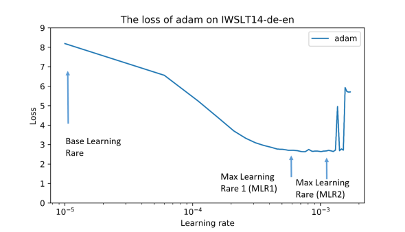
Figure 1: Range test curve for the IWSLT2014-de-en dataset, showing the chosen base and max learning rate for the triangular policy.

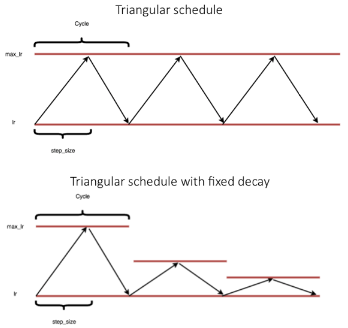
Figure 2: The learning rate decay used in our experiments.

Corpus	Train	Valid.	Test	Source Vocab.	Target Vocab.
IWSLT2014-de-en (DE2EN)	160,239	7,283	6,750	8,844	6,628
IWSLT2014-fr-en (FR2EN)	166,045	4,818	4,800	8,508	7,308
IWSLT2017-de-en (DE2EN)	192,347	4,829	4,822	13,156	10,108

Table 1: Datasets used for the experiment.

The CLR decay policy should be contrasted with the standard inverse square root policy (INV) that is commonly used in deep learning platforms, e.g., in fairseq (Ott et al., 2019). The inverse square root policy (INV) typically starts with a warm-up phase where the learning rate is linearly increased to a maximum value. The learning rate is decayed as the reciprocal of the square root of the number of epochs from the above-mentioned maximum value.

The other point of interest is how to deal with batch size when using CLR. Our primary interest is to use a larger batch size without compromising the generalization capability on the test set. Following the lead in Smith and Topin (2017), we look at how the NMT tasks perform when varying the batch size on top of the CLR policy. Compared to Smith and Topin (2017), we stretch the batch size range, going from batch size as small as 256 to as high as 4,096. Only through examining the extreme behaviors can we better understand the effect of batch size superimposed on CLR.

4 Experiments

4.1 Experiment Settings

The purpose of this section is to demonstrate the effects of applying CLR and various batch sizes to train NMT models. The experiments are performed on two translation directions (DE $\rightarrow$ EN and FR $\rightarrow$ EN) for IWSLT2014 and IWSLT2017 (Cettolo et al., 2012).

The data are pre-processed using functions from Moses (Koehn et al., 2007). The punctuation is normalized into a standard format. After tokenization, byte pair encoding (BPE) (Sennrich et al., 2016) is applied to the data to mitigate the adverse effects of out-of-vocabulary (OOV) rare words. The sentences with a source-target sentence length ratio greater than 1.5 are removed to reduce potential errors from sentence misalignment. Long sentences with a length greater than 250 are also removed as a common practice. The split of the datasets produces the training, validation (valid.) and test sets presented in Table 1.

Hyperparameters	Values
Encoder/Decoder Layers	6
Embedding Units	512
Attention Heads	4
Feed-forward Hidden Units	1,024
Batch Size (default)	4,096
Training Epoch (default)	50

Table 2: Hyperparameters for the experiments.

The transformer architecture (Vaswani et al., 2017) from fairseq (Ott et al., 2019) is used for all the experiments. The hyperparameters are presented in Table 2. We compared training under CLR with an inverse square for two popular optimizers used in machine translation tasks, Adam and SGD. All models are trained using one NVIDIA V100 GPU.

Corpus	Adam		SGD
	Max	Base	Max	Base
IWSLT2014-de-en	5.00E-04	1.00E-05	6.90E+00	1.00E-03
IWSLT2014-fr-en	8.00E-04	1.00E-05	-	-
IWSLT2017-de-en	7.60E-04	1.00E-05	8.00E+00	1.00E-03

Table 3: Learning rate boundary for CLR.

The learning rate boundary of the CLR is selected by the range test (shown in Figure 1). The base and maximal learning rates adopted in this study are presented in Table 3. Shrink strategy is applied when examining the effects of CLR in training NMT. The optimizers (Adam and SGD) are assigned with two options: 1) without shrink (as “nshrink”); 2) with shrink at a rate of 0.5 (“yshrink”), which means the maximal learning rate for each cycle is reduced at a decay rate of 0.5.

4.2 Effects of Applying CLR to NMT Training

A hypothesis we hold is that NMT training under CLR may result in a better local minimum than that achieved by training with the default learning rate schedule. A comparison experiment is performed for training NMT models for “IWSLT2014-de-en” corpus using CLR and INV with a range of initial learning rates on two optimizers (Adam and SGD), respectively. It can be observed that both Adam and SGD are very sensitive to the initial learning rate under the default INV schedule before CLR is applied (as shown in Figures 3 and 4). In general, SGD prefers a bigger initial learning rate when CLR is not applied. The initial learning rate of Adam is more concentrated towards the central range.

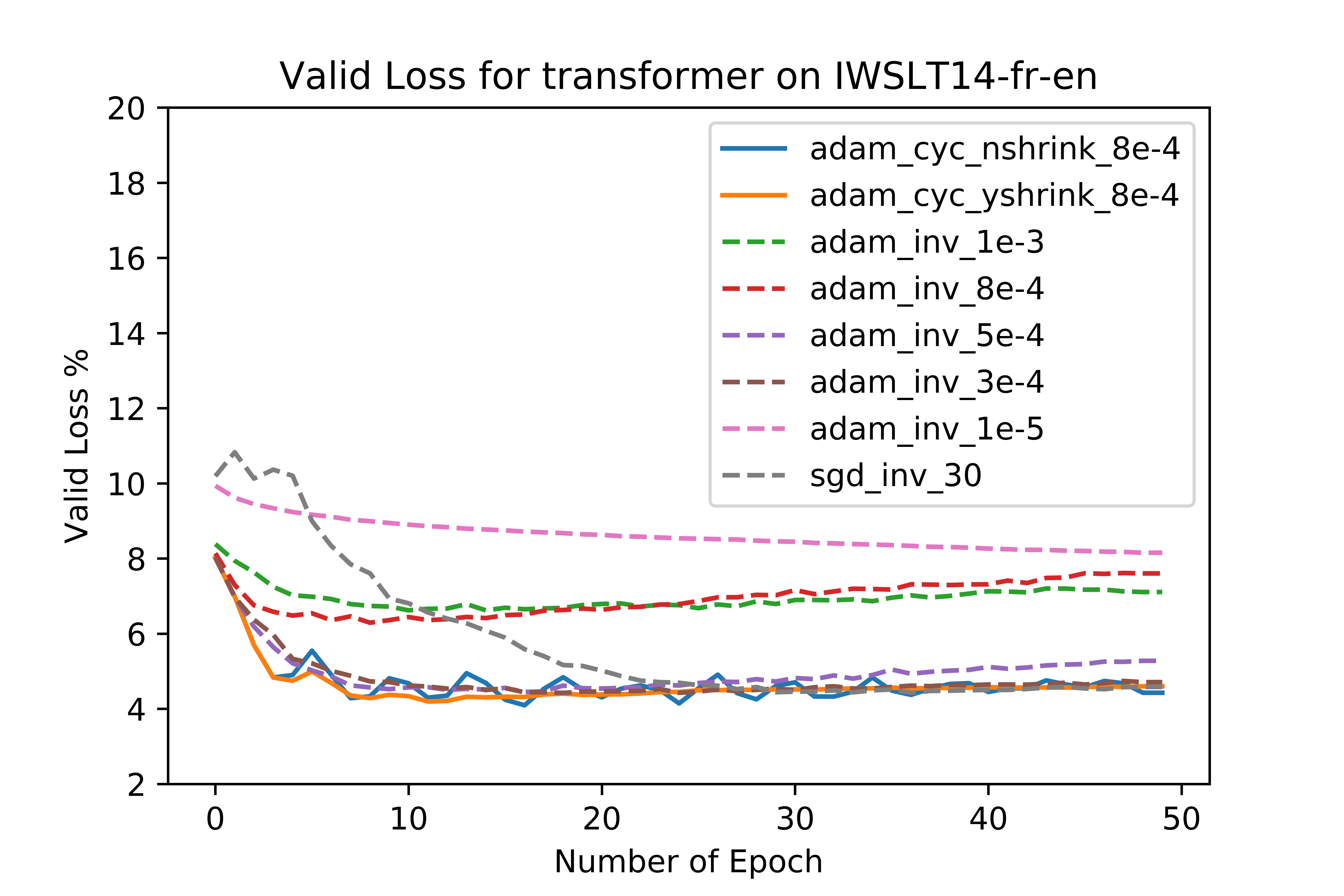
Figure 12: Effects of applying CLR to training NMT on IWSLT2014-fr-en.

Applying CLR has positive impacts on NMT training for both Adam and SGD. When applied to SGD, CLR exempts the needs for a big initial learning rate as it enables the optimizer to explore the local minima better. Shrinking on CLR for SGD is not desirable as a higher learning rate is required (Figure 4). It is noted that applying CLR to Adam produces consistent improvements regardless of shrink options (Figure 3). Furthermore, it can be observed that the effects of applying CLR to Adam are more significant than those of SGD, as shown in Figure 5. Similar results are obtained from our experiments on “IWSLT2017-de-en” and “IWSLT2014-fr-en” corpora (Figures 11 and 12 in Appendix A). The corresponding BLEU scores are presented in Table 4, in which the above-mentioned effects of CLR on Adam can also be established. The training takes fewer epochs to converge to reach a local minimum with better BLEU scores (i.e., bold fonts in Table 4).

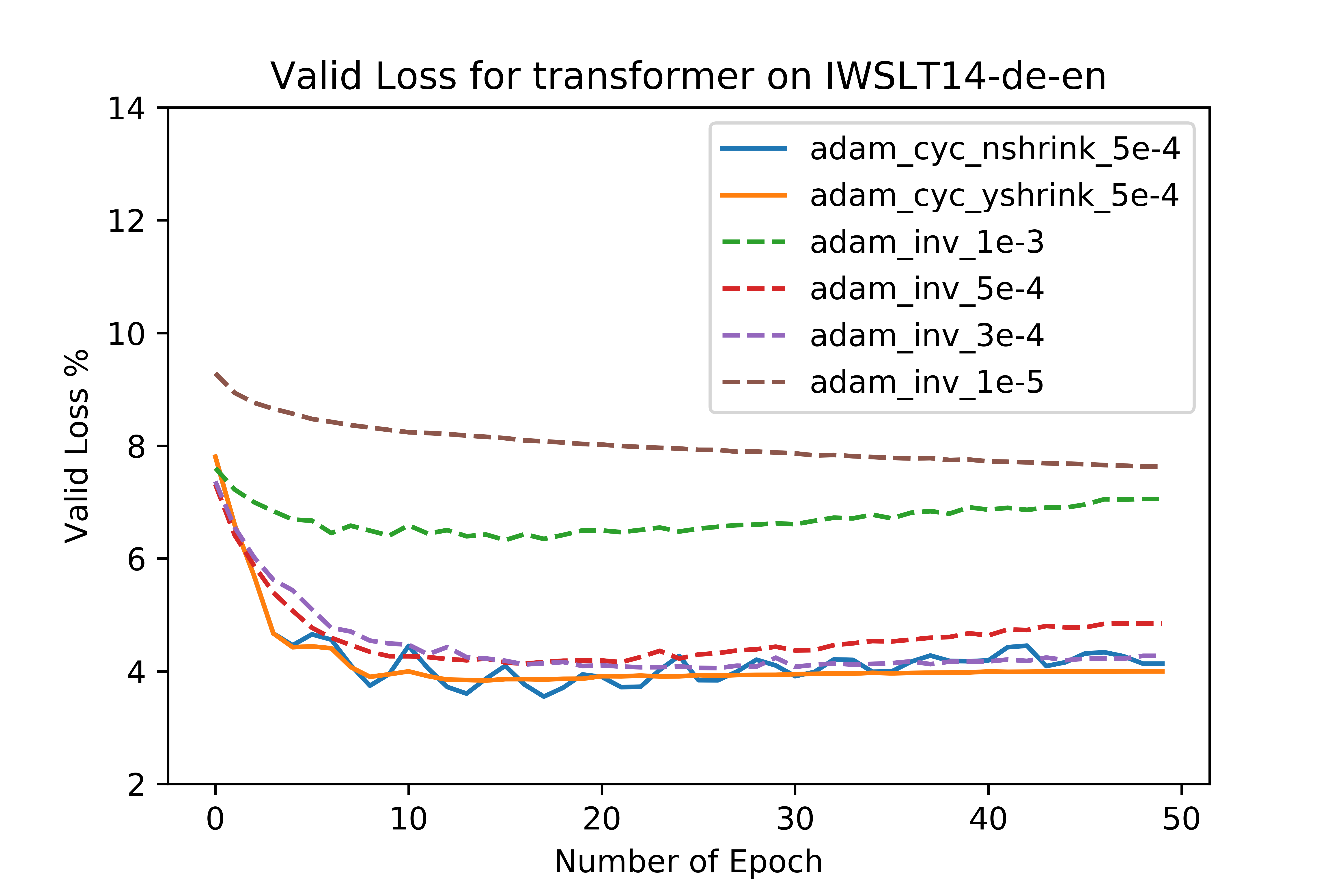
Figure 3: A comparison study of training NMT models on IWSLT2014-de-en using CLR and INV with a range of initial learning rate on Adam. The learning rate policy “adam_cyc_nshink_5e-4” denotes the optimizer Adam is trained under CLR with the no shrink option and a max learning rate of 5e-4.

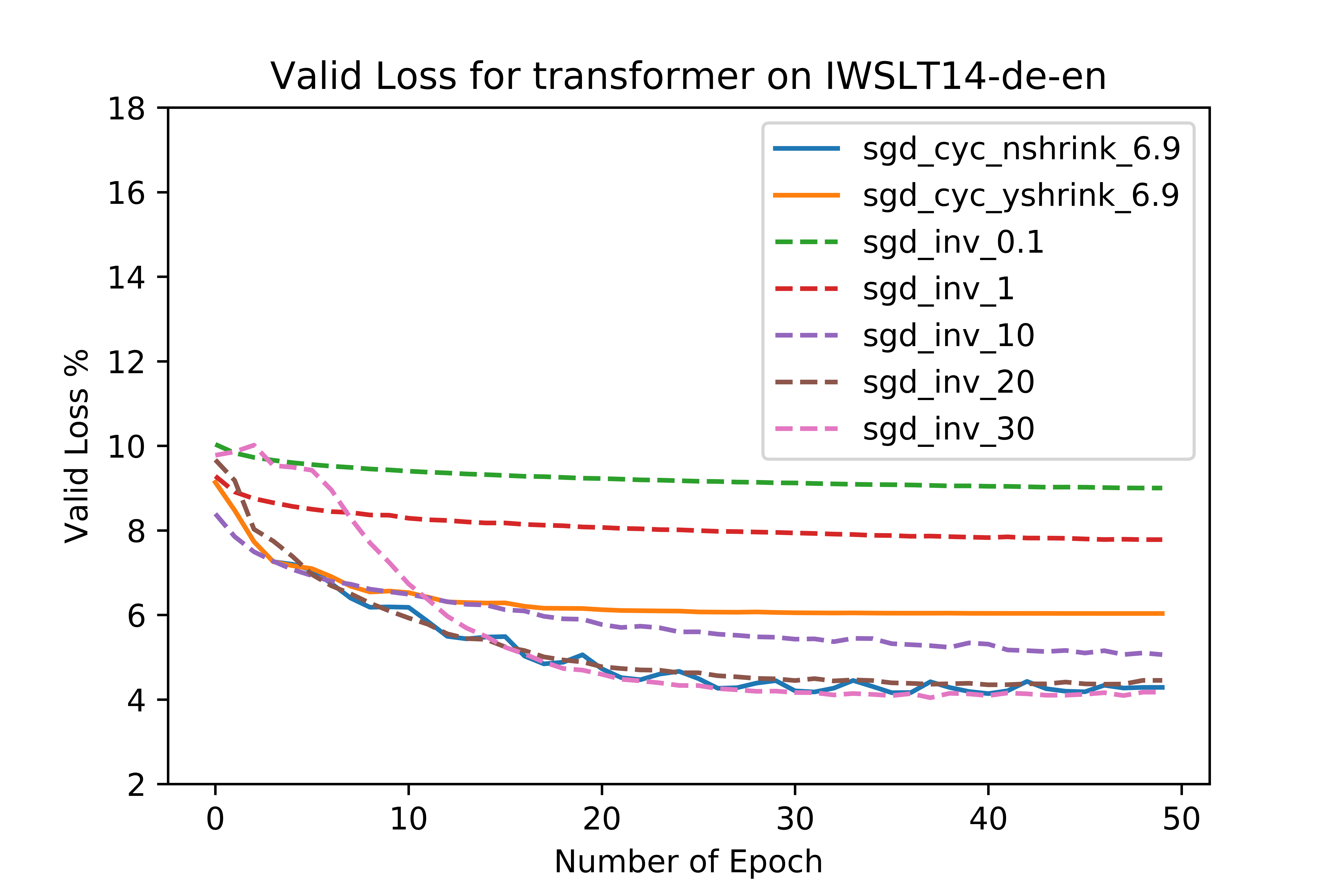
Figure 4: A comparison study of training NMT models on IWSLT2014-de-en using CLR and INV with a range of initial learning rate on SGD. The learning rate policy “sgd_cyc_yshink_5e-4” denotes the optimizer SGD is trained under CLR with the shrink option and a max learning rate of 5e-4.

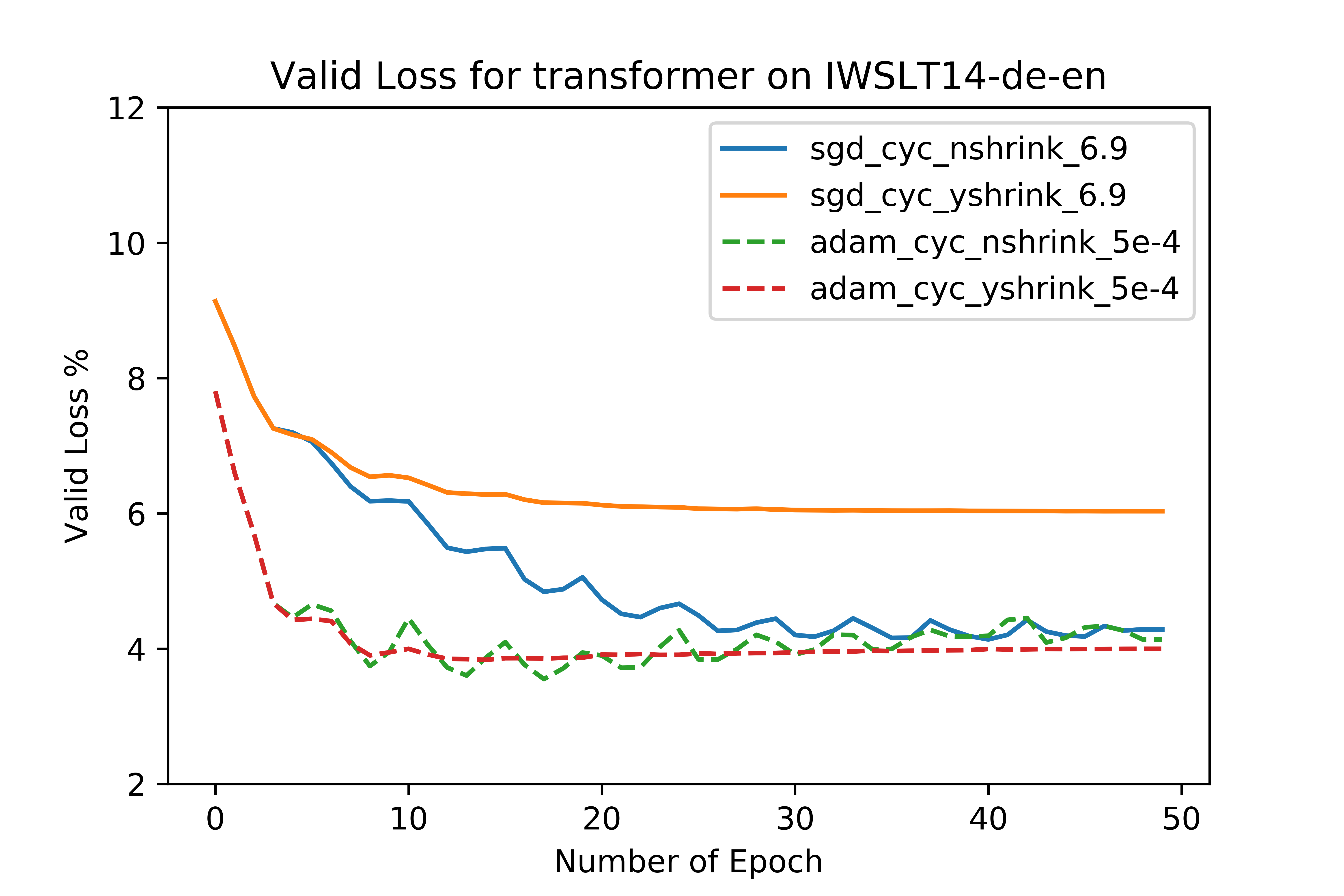
Figure 5: A view of effects of applying CLR to Adam and SGD when training the NMT on IWSLT2014-de-en.

Corpus	Learning Rate Policy	Best BLEU	Epoch
IWSLT2014-de-en	adam_cyc_nshrink_5e-4	32.65	18
	adam_cyc_yshrink_5e-4	31.29	18
	adam_inv_5e-4	30.88	16
	sgd_inv_30	30.78	42
	adam_inv_3e-4	30.46	34
	sgd_cyc_nshrink_6.9	30.16	45
IWSLT2017-de-en	adam_cyc_nshrink_7.6e-4	33.00	18
	adam_cyc_yshrink_7.6e-4	31.56	19
	sgd_inv_30	30.82	49
	adam_inv_3e-4	30.78	35
	adam_inv_5e-4	30.70	19
	sgd_cyc_nshrink_8	30.40	49
	adam_inv_7.6e-4	28.94	40
IWSLT2014-fr-en	adam_cyc_nshrink_8e-4	37.82	17
	adam_cyc_yshrink_8e-4	36.91	17
	adam_inv_5e-4	36.43	17
	adam_inv_3e-4	36.25	35
	sgd_inv_30	35.51	45
	adam_inv_8e-4	6.20	43

Table 4: The best BLEU for various learning rate policies when training NMT models on IWSLT2014-de-en, IWSLT2017-de-e and IWSLT2014-fr-en. The total number of training epochs for all the experiments is 50. The table is sorted by the best BLEU in descending order.

4.3 Effects of Batch Size on CLR

Batch size is regarded as a significant factor influencing deep learning models from the various CV studies detailed in Section 1. It is well known to CV researchers that a large batch size is often associated with a poor test accuracy. However, the trend is reversed when the CLR policy is introduced by Smith and Topin (2017). The critical question is: does this trend of using larger batch size with CLR hold for training transformers in NMT? Furthermore, what range of batch size does the associated regularization becomes significant? This will have implications because if CLR allows using a larger batch size without compromising the generalization capability, then it will allow training speed up by using a larger batch size. From Figure 6, we see that the trend of CLR with a larger batch size for NMT training does indeed lead to better performance. Thus the phenomenon we observe in Smith and Topin (2017) for CV tasks can be carried across to NMT. In fact, using a small batch size of 256 (the green curve in Figure 6) leads to divergence, as shown by the validation loss spiraling out of control. This is in line with the need to prevent over regularization when using CLR; in this case, the small batch size of 256 adds a strong regularization effect and thus need to be avoided. This larger batch size effect afforded by CLR is certainly good news because NMT typically deals with large networks and huge datasets. The benefit of a larger batch size afforded by CLR means that training time can be cut down considerably.

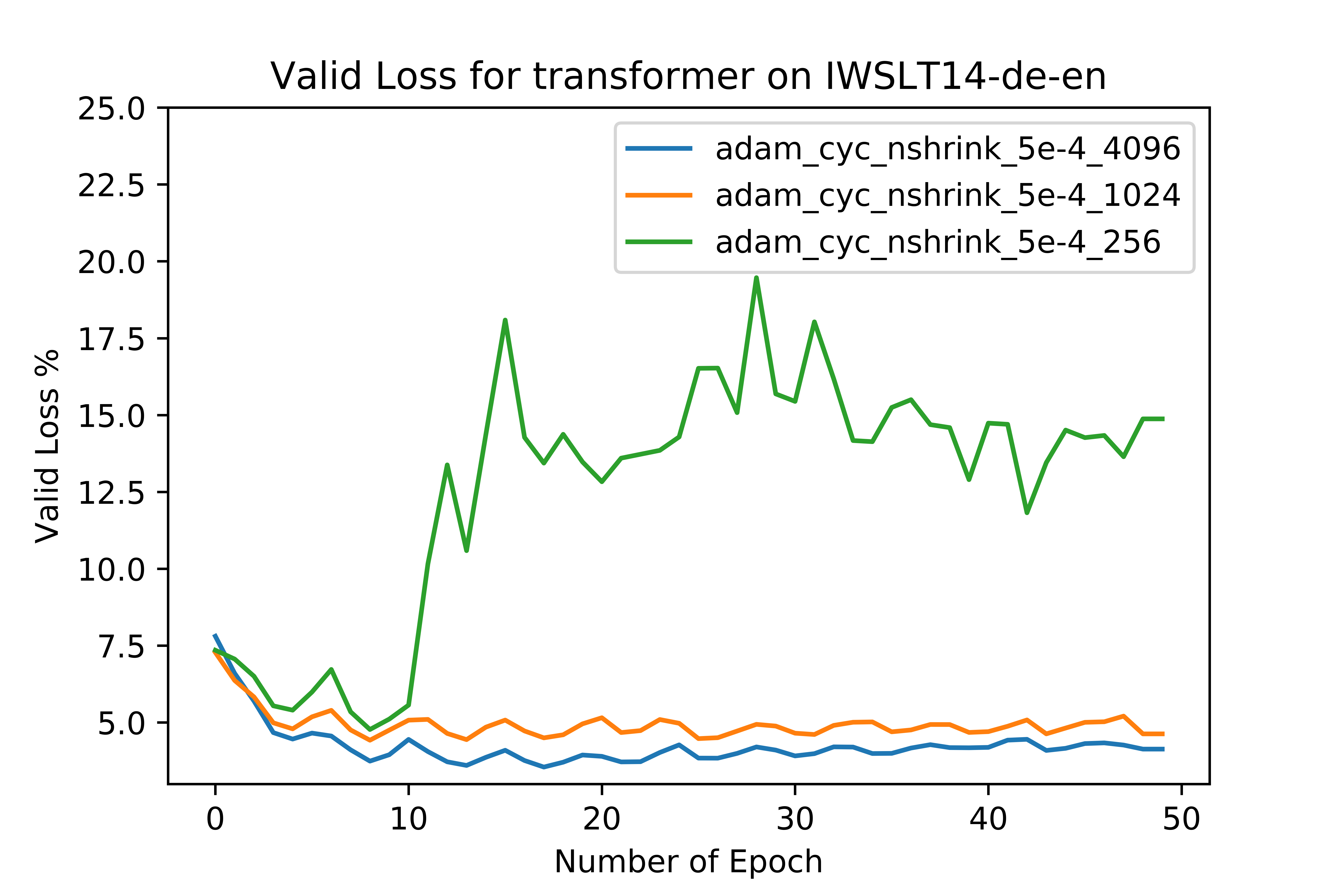
Figure 6: Effects of various batch sizes when training the NMT on IWSLT2014-de-en corpus with CLR.

5 Further Analysis

We observe the qualitative different range test curves for CV and NMT datasets. As we can see from Figures 1 and 7. The CV range test curve looks more well defined in terms of choosing the max learning rate from the point where the curve starts to be ragged. For NMT, the range curve exhibits a smoother, more plateau characteristic. From Figure 1, one may be tempted to exploit the plateau characteristic by choosing a larger learning rate on the extreme right end (before divergence occurs) as the triangular policy’s max learning rate. From our experiments and empirical observations, this often leads to the loss not converging due to excessive learning rate. It is better to be more conservative and choose the point where the loss stagnates as the max learning rate for the triangular policy.

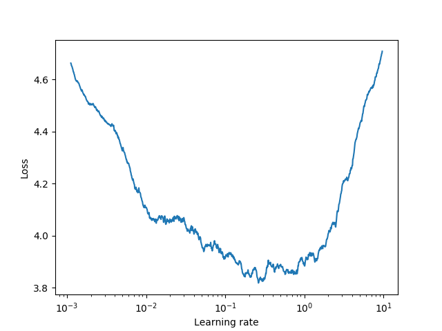
Figure 7: Range test curve for the CV CIFAR-100 dataset.

5.1 How to Apply CLR to NMT Training Matters

A range test is performed to identify the max learning rates (MLR1 and MLR2) for the triangular policy of CLR (Figure 1). The experiments showed the training is sensitive to the selection of MLR. As the range curve for training NMT models is distinctive to that obtained from a typical case of computer vision, it is not clear how to choose the MLR when applying CLR. A comparison experiment is performed to try MLRs with different values. It can be observed that MLR1 is a preferable option for both SGD and Adam (Figures 8 and 9). The “noshrink” option is mandatory for SGD, but this constraint can be relaxed for Adam. Adam is sensitive to excessive learning rate (MLR2).

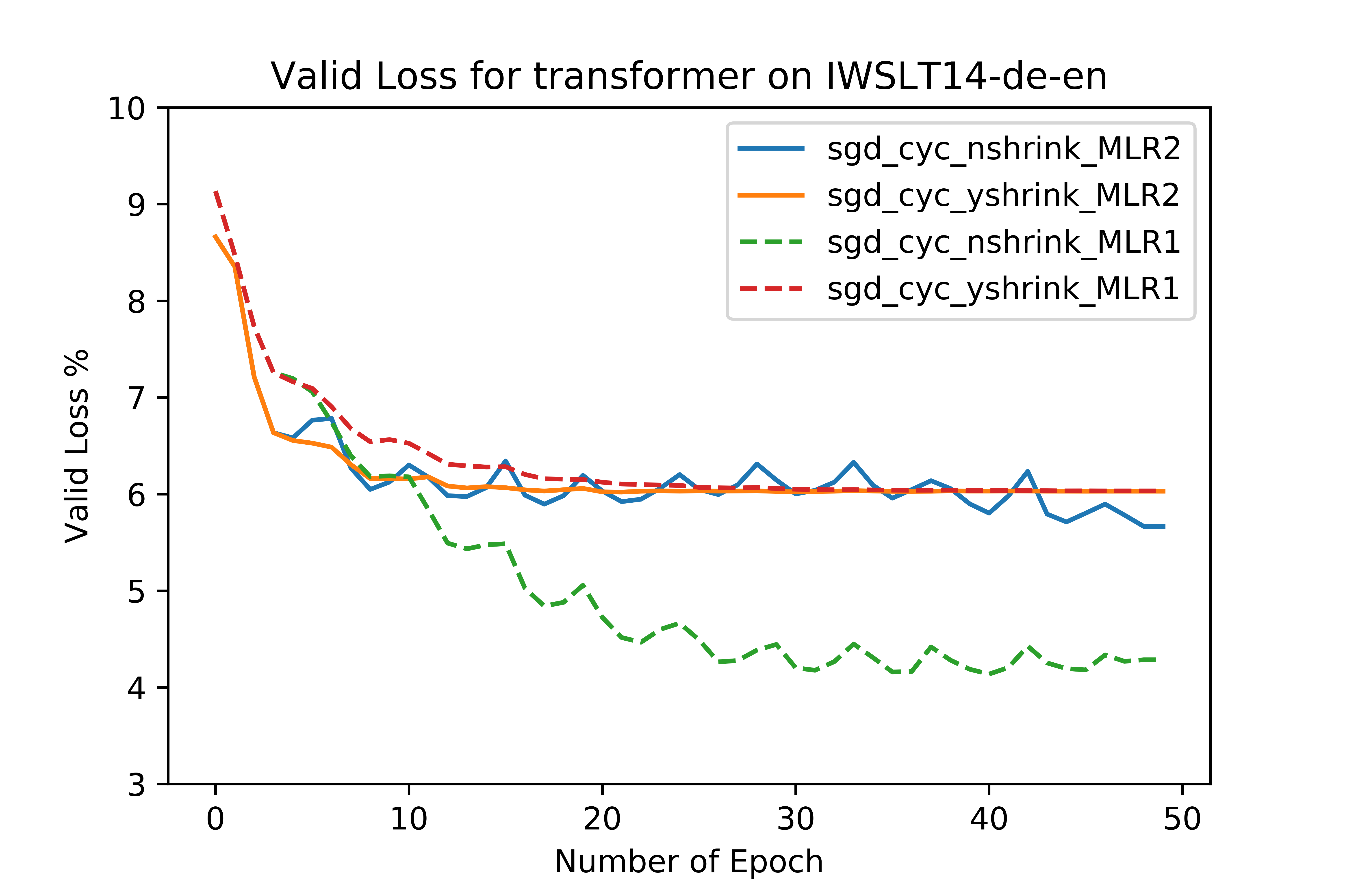
Figure 8: MLR1 with “noshrink” is a preferable option for SGD when applying CLR to train NMT models on IWSLT2014-de-en.

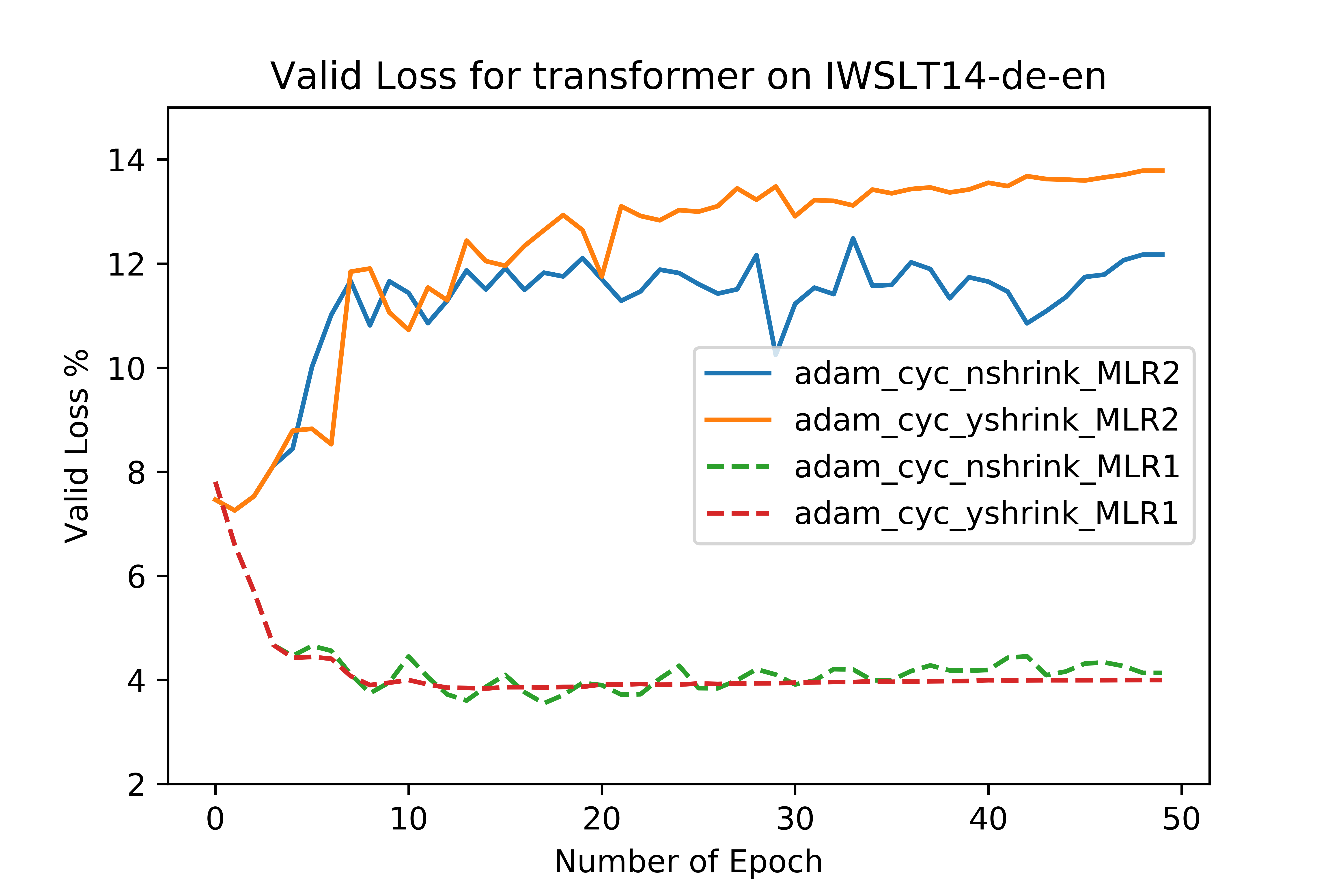
Figure 9: MLR1 is a preferable option for Adam when applying CLR to train NMT models on IWSLT2014-de-en.

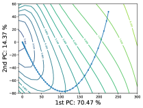
(a) adam-inv-1e-3

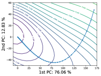
(b) adam-inv-5e-4

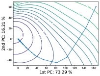
(c) adam-cyc-yshrink

Figure 10: Loss surface, optimizer trajectory and learning rates visualization for training NMT models on IWSLT2014-de-en.

5.2 Rationale behind Applying CLR to NMT Training

There are two reasons proposed in Smith (2015) on why CLR works. The theoretical perspective proposed is that the increasing learning rate helps the optimizer to escape from saddle point plateaus. As pointed out in Dauphin et al. (2015), the difficulty in optimizing deep learning networks is due to saddle points, not local minima. The other more intuitive reason is that the learning rates covered in CLR are likely to include the optimal learning rate, which will be used throughout the training. Leveraging the visualization techniques proposed by Li et al. (2017), we take a peek at the error surface, optimizer trajectory and learning rate. The first thing to note is the smoothness of the error surface. This is perhaps not so surprising given the abundance of skip connections in transformer-based networks. Referring to Figure 10 (c), we see the cyclical learning rate greatly amplifying Adam’s learning rate in flatter region while nearer the local minimum, the cyclical learning rate policy does not harm convergence to the local minimum. This is in contrast to Figure 10 (a) and (b), where although the adaptive nature of the learning rate in Adam helps to move quickly across flatter region, the effect is much less pronounced without the cyclical learning rate. Figure 10 certainly does give credence to the hypothesis that the cyclical learning rate helps to escape saddle point plateaus, as well as the optimal learning rate will be included in the cyclical learning rate policy.

Some explanation about Figure 10 is in order here. Following Li et al. (2017), we first assemble the network weight matrix by concatenating columns of network weights at each epoch. We then perform a Principal Component Analysis (PCA) and use the first two components for plotting the loss landscape. Even though all three plots in Figure 10 seem to converge to the local minimum, bear in mind that this is only for the first two components, with the first two components contributing to 84.84%, 88.89% and 89.5% of the variance respectively. With the first two components accounting for a large portion of the variance, it is thus reasonable to use Figure 10 as a qualitative guide.

6 Conclusion

From the various experiment results, we have explored the use of CLR and demonstrated the benefits of CLR for transformer-based networks unequivocally. Not only does CLR help to improve the generalization capability in terms of test set results, but it also allows using larger batch size for training without adversely affecting the generalization capability. Instead of just blindly using default optimizers and learning rate policies, we hope to raise awareness in the NMT community the importance of choosing a useful optimizer and an associated learning rate policy.

Appendix A Appendices

Figures 11,  12 are included in this Appendix.

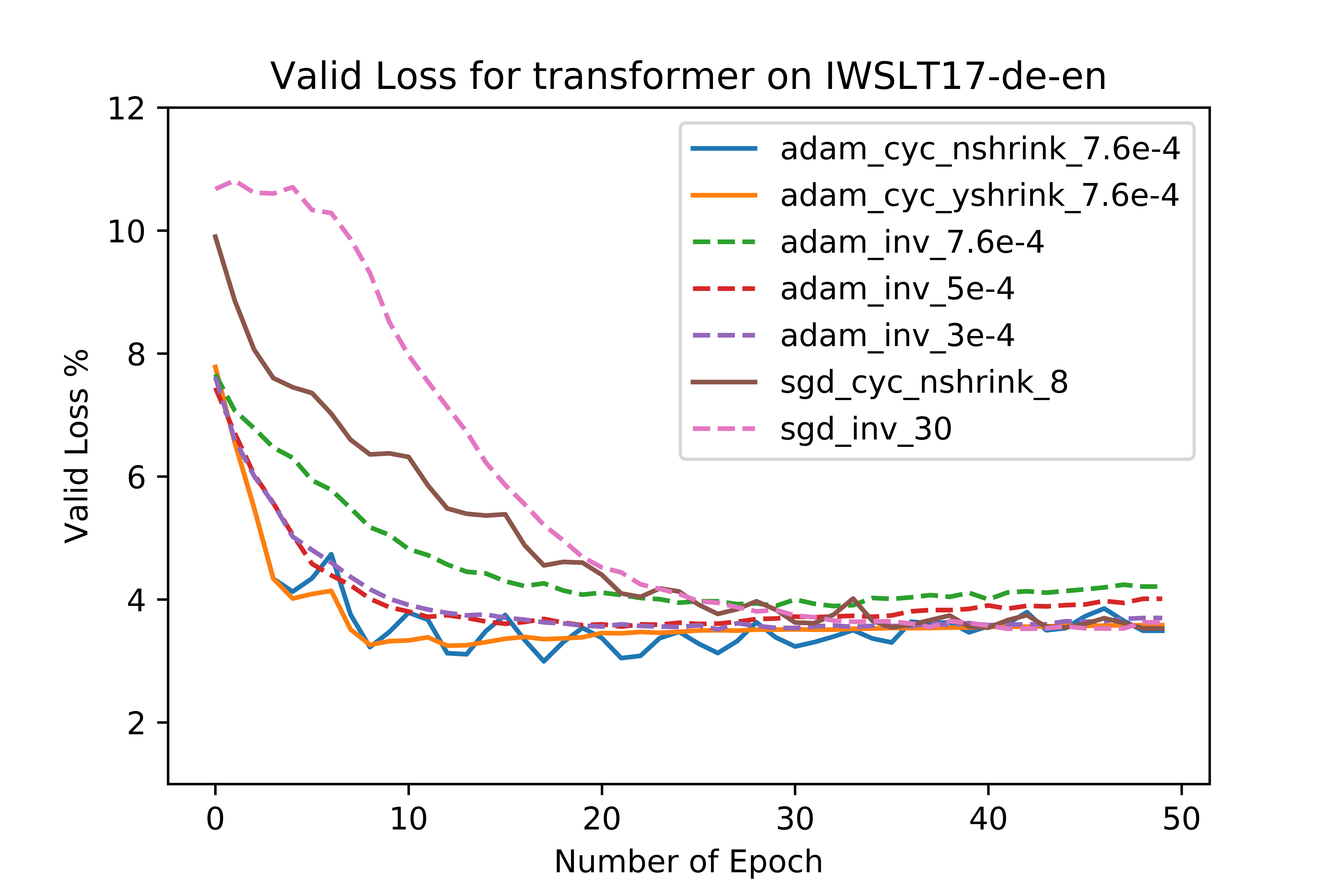
Figure 11: Effects of applying CLR to training NMT on IWSLT2017-de-en.

Appendix B Supplemental Material

Scripts and data are available at https://github.com/nlp-team/CL_NMT.

References

- Aarts and Korst (2003) Ehl Emile Aarts and Jhm Jan Korst. 2003. Simulated annealing and boltzmann machines.
- Bengio et al. (2009) Yoshua Bengio, Jérôme Louradour, Ronan Collobert, and Jason Weston. 2009. Curriculum learning. In ICML.
- Bottou (2010) Léon Bottou. 2010. Large-scale machine learning with stochastic gradient descent.
- Cettolo et al. (2012) Mauro Cettolo, Christian Girardi, and Marcello Federico. 2012. Wit3: Web inventory of transcribed and translated talks. In Proceedings of the 16th Conference of the European Association for Machine Translation (EAMT), pages 261–268, Trento, Italy.
- Chung et al. (2014) Junyoung Chung, Çaglar Gülçehre, Kyunghyun Cho, and Yoshua Bengio. 2014. Empirical evaluation of gated recurrent neural networks on sequence modeling. ArXiv, abs/1412.3555.
- Dauphin et al. (2015) Yann Dauphin, Harm de Vries, and Yoshua Bengio. 2015. Equilibrated adaptive learning rates for non-convex optimization. In NIPS.
- Devlin et al. (2019) Jacob Devlin, Ming-Wei Chang, Kenton Lee, and Kristina Toutanova. 2019. Bert: Pre-training of deep bidirectional transformers for language understanding. In NAACL-HLT.
- Dinh et al. (2017) Laurent Dinh, Razvan Pascanu, Samy Bengio, and Yoshua Bengio. 2017. Sharp minima can generalize for deep nets. ArXiv, abs/1703.04933.
- Duchi et al. (2010) John C. Duchi, Elad Hazan, and Yoram Singer. 2010. Adaptive subgradient methods for online learning and stochastic optimization. J. Mach. Learn. Res., 12:2121–2159.
- He et al. (2015) Kaiming He, Xiangyu Zhang, Shaoqing Ren, and Jian Sun. 2015. Deep residual learning for image recognition. 2016 IEEE Conference on Computer Vision and Pattern Recognition (CVPR), pages 770–778.
- Hochreiter and Schmidhuber (1997a) Sepp Hochreiter and Jürgen Schmidhuber. 1997a. Flat minima. Neural Computation, 9:1–42.
- Hochreiter and Schmidhuber (1997b) Sepp Hochreiter and Jürgen Schmidhuber. 1997b. Long short-term memory. Neural Computation, 9:1735–1780.
- Huang et al. (2016) Gao Huang, Zhuang Liu, and Kilian Q. Weinberger. 2016. Densely connected convolutional networks. 2017 IEEE Conference on Computer Vision and Pattern Recognition (CVPR), pages 2261–2269.
- Keskar et al. (2016) Nitish Shirish Keskar, Dheevatsa Mudigere, Jorge Nocedal, Mikhail Smelyanskiy, and Ping Tak Peter Tang. 2016. On large-batch training for deep learning: Generalization gap and sharp minima. ArXiv, abs/1609.04836.
- Kingma and Ba (2014) Diederik P. Kingma and Jimmy Ba. 2014. Adam: A method for stochastic optimization. CoRR, abs/1412.6980.
- Koehn et al. (2007) Philipp Koehn, Hieu Hoang, Alexandra Birch, Chris Callison-Burch, Marcello Federico, Nicola Bertoldi, Brooke Cowan, Wade Shen, Christine Moran, Richard Zens, Chris Dyer, Ondrej Bojar, Alexandra Constantin, and Evan Herbst. 2007. Moses: Open source toolkit for statistical machine translation. In Proceedings of the 45th Annual Meeting of the Association for Computational Linguistics Companion Volume Proceedings of the Demo and Poster Sessions, pages 177–180, Prague, Czech Republic. Association for Computational Linguistics.
- Krizhevsky et al. (2017) Alex Krizhevsky, Ilya Sutskever, and Geoffrey E. Hinton. 2017. Imagenet classification with deep convolutional neural networks. Commun. ACM, 60:84–90.
- Li et al. (2017) Hao Li, Zheng Xu, Gavin Taylor, and Tom Goldstein. 2017. Visualizing the loss landscape of neural nets. In NeurIPS.
- Liu et al. (2019) Liyuan Liu, Haoming Jiang, Pengcheng He, Weizhu Chen, Xiaodong Liu, Jianfeng Gao, and Jiawei Han. 2019. On the variance of the adaptive learning rate and beyond. ArXiv, abs/1908.03265.
- Luo et al. (2019) Liangchen Luo, Yuanhao Xiong, Yan Liu, and Xu Sun. 2019. Adaptive gradient methods with dynamic bound of learning rate. ArXiv, abs/1902.09843.
- McCandlish et al. (2018) Sam McCandlish, Jared Kaplan, Dario Amodei, and OpenAI Dota Team. 2018. An empirical model of large-batch training. ArXiv, abs/1812.06162.
- Ott et al. (2019) Myle Ott, Sergey Edunov, Alexei Baevski, Angela Fan, Sam Gross, Nathan Ng, David Grangier, and Michael Auli. 2019. fairseq: A fast, extensible toolkit for sequence modeling. In Proceedings of NAACL-HLT 2019: Demonstrations.
- Reddi et al. (2018) Sashank J. Reddi, Satyen Kale, and Sanjiv Kumar. 2018. On the convergence of adam and beyond. ArXiv, abs/1904.09237.
- Sennrich et al. (2016) Rico Sennrich, Barry Haddow, and Alexandra Birch. 2016. Neural machine translation of rare words with subword units. In Proceedings of the 54th Annual Meeting of the Association for Computational Linguistics (Volume 1: Long Papers), pages 1715–1725, Berlin, Germany. Association for Computational Linguistics.
- Simonyan and Zisserman (2014) Karen Simonyan and Andrew Zisserman. 2014. Very deep convolutional networks for large-scale image recognition. CoRR, abs/1409.1556.
- Smith (2015) Leslie N. Smith. 2015. Cyclical learning rates for training neural networks. 2017 IEEE Winter Conference on Applications of Computer Vision (WACV), pages 464–472.
- Smith and Topin (2017) Leslie N. Smith and Nicholay Topin. 2017. Super-convergence: Very fast training of residual networks using large learning rates. ArXiv, abs/1708.07120.
- Vaswani et al. (2017) Ashish Vaswani, Noam Shazeer, Niki Parmar, Jakob Uszkoreit, Llion Jones, Aidan N Gomez, Ł ukasz Kaiser, and Illia Polosukhin. 2017. Attention is all you need. In I. Guyon, U. V. Luxburg, S. Bengio, H. Wallach, R. Fergus, S. Vishwanathan, and R. Garnett, editors, Advances in Neural Information Processing Systems 30, pages 5998–6008. Curran Associates, Inc.
- Zhang et al. (2019) Michael Ruogu Zhang, James Lucas, Geoffrey E. Hinton, and Jimmy Ba. 2019. Lookahead optimizer: k steps forward, 1 step back. ArXiv, abs/1907.08610.