Deep Multilayer Perceptrons for Dimensional
Speech Emotion Recognition

Abstract

Modern deep learning architectures are ordinarily performed on high-performance computing facilities due to the large size of the input features and complexity of its model. This paper proposes traditional multilayer perceptrons (MLP) with deep layers and small input size to tackle that computation requirement limitation. The result shows that our proposed deep MLP outperformed modern deep learning architectures, i.e., LSTM and CNN, on the same number of layers and value of parameters. The deep MLP exhibited the highest performance on both speaker-dependent and speaker-independent scenarios on IEMOCAP and MSP-IMPROV corpus.

I Introduction

Speech emotion recognition is currently gaining interest from both academia and commercial industries. Researchers in the affective computing field progressively proposed new methods to improve the accuracy of automatic emotion recognition. Commercial industries are trying to make this technology available to the market since its potential applications. Previously, researchers has attempted to implement speech-based emotion recognition for wellbeing detection [1], call center application [2], and automotive safety [3].

One of the common requirements in computing speech emotion recognition is the availability of high-performance computing since the dataset usually is very large in size, and the classifying methods are complicated. Graphical processing units (GPU)-based computers are often used over CPU-based computers due to its processing speed to process the data, particularly, image-like data.

This paper proposes the use of deep multilayer perceptrons (MLP) to overcome the requirement of high computing power required by modern deep learning architectures. The inputs are high-level statistical functions (HSF), which are used to reduce the dimension of input features. The outputs are emotion dimensions, i.e., degree of valence, arousal, and dominance.

According to research in psychology, dimensional emotion is another view in emotion theories apart from categorical emotion. Russel [4] argued that emotion categories could be derived from this dimensional emotion, particularly in valence-arousal space. Given the benefit of the ability to convert dimensional emotion to categorical emotion, but not vice versa, predicting the emotion dimension is more beneficial than predicting the emotion category. We added dominance, since it is suggested in [5], and the availability of those labels in the datasets. Dimensional emotion recognition are evaluated with deep MLP from speech data since the target applications are speech-based technology like call center and voice assistant applications.

The contribution of this paper is the evaluation of the classical MLP technique with deep layers compared with modern deep learning techniques, i.e., LSTM and CNN, in terms of concordance correlation coefficient (CCC). The deep neural network is an extension of the neural network with deeper layers, commonly five or more layers [6]. Our results show that on both speaker-dependent and speaker-independent, in three datasets, deep MLP obtained higher performances than LSTM and CNN. The proposed method worked effectively on the small size of feature, in which, this may be a limitation of our proposed deep MLP method.

II Data and Feature Sets

In this section, we describe data and feature sets used in this research.

IEMOCAP

The interactive emotional dyadic motion capture database is used in this research [7]. Although the database consists of the measurement of speech, facial expression, head, and movements of affective dyadic sessions, only speech data are processed. The database contains approximately 12 h of data with 10039 utterances. All of those data are used. The dimensional emotion labels are given in valence, arousal, and dominance, in range [1-5] score and normalized into [-1, 1] as in [8] when those labels are fed into the neural network system. For speech data, two versions are available in the dataset, stereo data per dialog and mono data per sentence (utterance). We used the mono version since it is easy to process with the labels. The sampling rate of the data was 16 kHz and 16-bit PCM.

We arranged the IEMOCAP dataset into two scenarios, speaker-dependent (SD) and speaker-independent. On speaker-independent, we split the dataset with ratio 80/20 for training/test set, while in speaker-independent, the last session, i.e., session five, is left for the test set (leave one session out, LOSO). The ratio of dataset partition in the speaker-independent scenario is similar to speaker-dependent split which is shown in Table I.

MSP-IMPROV

We used the MSP-IMPROV corpus to generalize the impact of the evaluated methods. MSP-IMPROV is an acted corpus of dyadic interactions to study emotion perception. This dataset consists of speech and visual recording of 18 hours of affective dyadic sessions. Same as IEMOCAP dataset, we only used the speech data, with 8438 utterances. The same split ratio is used in speaker-dependent scenario while the last session six is used for test set in in speaker-independent scenario, with the same labels scale and normalization. While IEMOCAP labels are annotated by at least two subjects, these MSP-IMPROV labels are annotated by at least five annotators. The speech data were mono, 44 kHz, and 16-bit PCM.

Table I shows the number of utterances allocated for each set partition for both speaker-dependent and speaker-independent, including MSP-IMPROV dataset.

Mixed-corpus

In addition to the two datasets above, we mixed those two datasets to create a new category of dataset namely mixed-corpus. In mixed-corpus, we concatenated speaker-dependent from IEMOCAP with speaker-dependent from MSP-IMPROV for each, training, development and test sets. The same rules also applied for the speaker-independent scenario.

TABLE I: Number of utterances used in the datasets on each partition

Scenarios	Training	Development	Test
IEMOCAP-SD	6431	1608	2000
IEMOCAP-LOSO	6295	1574	2170
IMPROV-SD	5256	1314	1868
IMPROV-LOSO	5452	1364	1622

Acoustic Feature Set

We used high statistical functions of the low-level descriptor (LLD) from Geneva Minimalistic Acoustic Parameter Set (GeMAPS), which is developed by Eyben et al. [9]. The HSF features are extracted per utterance depend on the given labels, while the LLDs are processed on a frame-based level with 25 ms window size and 10 ms of hop size. The use of HSF feature reduce computation complexity since the feature size decrease from (3409 $\times$ 23) to (1 $\times$ 23 features), that is, for IEMOCAP dataset. To obtain the HSF feature, however, LLDs must obtained first. Then, HSF can be calculated as statistics of those LLDs for a fixed time, in this case, per utterance.

TABLE II: GeMAPS feature [9] and its functionals; only functionals (HSFs) used in this dimensional SER.

LLDs	loudness, alpha ratio, hammarberg index, spectral slope 0-500 Hz, spectral slope 500-1500 Hz, spectral flux, 4 MFCCs, F0, jitter, shimmer, Harmonics-to-Noise Ratio (HNR), Harmonic difference H1-H2, Harmonic difference H1-A3, F1, F1 bandwidth, F1 amplitude, F2, F2 amplitude, F3, and F3 amplitude.
HSFs	mean (of LLDs), standard deviation (of LLDs), silence

To add those functionals, we used a silence feature, which is also extracted per utterance. Silence feature, in this paper, is defined as the portion of the silence frames compared to the total frames in an utterance. In human-human communication, this portion of silence in speaking depends on the speaker’s emotion. For example, high arousal emotion category like happy may have fewer silences (or pauses) than a sad emotion category. The ratio of silence per utterance is calculated as

$$S=\frac{N_{s}}{N_{t}},$$ (1)

where $N_{s}$ is the number of frames to be categorized as silence (silence frames), and $N_{t}$ is the number of total frames within an utterance. To be categorized as silence, a frame is checked whether it is less than a threshold, which is a multiplication of a factor with a root mean square (RMS) energy ($X_{rms}$). This RMS energy is formulated as

$$th=0.3\times\overline{X_{rms}}$$ (2)

and $X_{rms}$ is defined as

$$X_{rms}=\sqrt{\frac{1}{n}\sum_{i=1}^{n}x[i]^{2}}$$ (3)

where silence factor of $0.3$ is obtained from experiments. These equations are similar to what is proposed in [10] and [11]. In [10], the author of that paper used a fixed threshold, while we evaluated some factors of to find the best factor for silence feature in speech emotion recognition. In [11], the author divided the total duration of disfluency over the total utterance length on $n$ words and counted it as a disfluency feature.

III Benchmarked and Proposed Method

We evaluated three different methods in this paper, LSTM, CNN and MLP. LSTM and CNN are used as baselines, while MLP with deep layers is the proposed method. All evaluated methods used the same numbers of layers, units and value of parameters.

III-A Benchmarked Methods: LSTM and CNN

LSTM and CNN are two common deep learning architectures widely used in speech emotion recognition [12, 13, 14]. We used those two architectures as the baselines due to its reported effectiveness on predicting valence, arousal, and dominance. Both LSTM and CNN evaluated here have the same five layers with the same number of units. For the size of the kernel in CNN architecture, we determined it in order that the number of trainable parameters is similar. The other parameters, like batch size, feature and label standardization, loss function, number of iterations, and callback criteria, are same for both architectures.

Fig. 1 shows both structures of LSTM and CNN. On the first layer, 256 neurons are used and decreased half for the next layers since the models are supposed to learn better along with those layers. Five LSTM layers used tanh as activation function, while five CNN layers used ReLU activation function. We kept all output from the last LTM layer and flatten it before splitting into three dense layers for obtaining the prediction of valence, arousal, and dominance. For the CNN architecture, the same flatten layer is used before entering three one-unit dense layers.

Both architectures used the same standardization for input features and labels. The z-score normalization is used to standardize feature, while minmax scaler is used to scale the labels into [0, 1] range. We used CCC [15] loss as the cost function with multitask (MTL) approach in which the prediction of valence, arousal, and dominance are done simultaneously. While CCC loss (CCCL) is used as the cost function, the following CCC is used to evaluate the performance of recognition.

$$CCC =\dfrac{2\rho\sigma_{x}\sigma_{y}}{\sigma_{x}^{2}+\sigma_{y}^{2}+(\mu_{x}-\mu_{y})^{2}}$$ (4)

$$CCCL =1-CCC$$ (5)

where $\rho$ is Pearson’s correlation between gold standard $y$ and and predicted score $x$, $\sigma$ is standard deviation, and $\mu$ is the mean score. The total loss ($L_{T}$) for three variables is then defined as the sum of CCCL for those three with corresponding weighting factors,

$$L_{T}=\alpha CCCL_{V}+\beta CCCL_{A}+(1-\alpha-\beta)CCCL_{D}$$ (6)

where $\alpha$ and $\beta$ are weighting factors for loss function of valence ($CCCL_{V}$) and arousal ($CCCL_{A}$), respectively. The weighting factors of loss function for dominance ($CCCL_{D}$) is obtained by subtracting 1 by the sum of those weighting factors. The CCC is used to evaluate all architectures including the proposed deep MLP method.

All architectures used a mini-batch size of 200 utterances by shuffling its orders, maximum number iteration of 180, and 10 iterations patience of early stopping criteria (callback). An adam optimizer [16] is used to adjust the learning rate during the training process. Both architectures run on GPU-based machine using CuDNN implementation [17] within Keras toolkit [18].

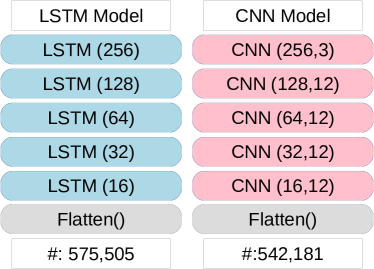
Figure 1: Diagram of LSTM and CNN used for benchmarking of proposed deep MLP; the number inside the bracket denoted the number of units (nodes); the second number on CNN denotes kernel size, # denotes number of trainable parameters.

III-B Proposed Method: Deep MLP

Fig. 2 shows our proposed deep MLP structure. The MLP used here similar to the definition of connectionist learning proposed by Hinton [19]. As the benchmarked methods, deep MLP also has five layers with the same number of units as previous. The only difference of the layer structure from the previous is the absent of flatten layer since the output of the last MLP layers can be coupled directly to three one-unit dense layers. While the previous LSTM and CNN used batch normalization layer in the beginning (input) to speed-up computation process, this deep MLP structure did not use that layer since the implementation only need a minute to run on a CPU-based machine.

We used the same batch size, tolerance for early stopping criteria, optimizer, and maximum number of iteration as the benchmarked methods. While the benchmarked methods used CCC the as loss function, the proposed deep MLP method used a mean square error (MSE) as the cost function,

$$MSE=\dfrac{1}{n}\sum_{i=1}^{n}(y_{i}-x_{i})^{2}.$$ (7)

The total loss function is given as an average of MSE scores from valence, arousal, and dominance,

$$MSE_{T}=\dfrac{1}{3}(MSE_{V}+MSE_{A}+MSE_{D}).$$ (8)

There are no weighting factors used here since we do not find a way to implement it via scikit-learn toolkit [20], in which the proposed deep MLP is implemented. The same reason applied for the selection of MSE over CCC for the loss function. The Python implementation codes for both proposed and benchmarked methods are available at https://github.com/bagustris/deep_mlp_ser.

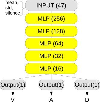
Figure 2: Diagram of proposed deep MLP with five layers; the number inside the bracket denoted the number of units.

IV Experiment Results and Discussion

CCC is the standard metric used in affective computing to measure the performance of dimensional emotion recognition. We presented our results in that metric in two different groups; within-corpus and mixed-corpus evaluation. The results are shown in Table III and IV.

Table III shows CCC scores of valence (V), arousal (A), dominance (D) and its average from different datasets, scenarios, and methods. The proposed deep MLP method outperforms benchmarked methods by remarkable margins. On every emotion dimensions and averaged score, the proposed deep MLP gained the highest CCC score for both speaker-dependent and speaker-independent scenarios (typed in bold). On IEMOCAP dataset, the score of speaker-dependent is only slightly higher than speaker-independent due to the nature of dataset structure. The utterances in IEMOCAP dataset is already in order by its session when it is sorted by file names. The change from speaker-dependent to speaker-independent is done by changing the number of train/test partitions. In contrast, the file naming of utterances in MSP-IMPROV made the arrangement of the sessions not in order when utterances are sorted by its file names. We did the sorting process to assure the pair of features and labels. The gap between speaker-dependent and speaker-independent in MSP-IMPROV is larger than in IEMOCAP which may be caused by those different files organization. A case where our deep MLP method gained a lower score is on dominance part of MSP-IMPROV speaker-dependent scenario, however, the averaged CCC score, in that case, is still the highest.

TABLE III: Results of CCC scores on within-corpus evaluation

Dataset	Method	V	A	D	Mean
IEMOCAP	speaker-dependent
	LSTM	0.222	0.508	0.432	0.387
	CNN	0.086	0.433	0.401	0.307
	MLP	0.335	0.599	0.473	0.469
	speaker-independent (LOSO)
	LSTM	0.210	0.474	0.394	0.359
	CNN	0.113	0.460	0.410	0.328
	MLP	0.316	0.488	0.454	0.453
MSP-IMPROV	speaker-dependent
	LSTM	0.392	0.629	0.524	0.515
	CNN	0.346	0.623	0.522	0.497
	MLP	0.438	0.650	0.519	0.536
	speaker-independent (LOSO)
	LSTM	0.210	0.483	0.313	0.335
	CNN	0.216	0.524	0.387	0.375
	MLP	0.269	0.551	0.401	0.407

Table IV shows the results from the mixed-corpus dataset. This corpus is concatenation of IEMOCAP with MSP-IMPROV as listed in Table I, for both speaker-dependent and speaker-independent scenarios. In this mixed-corpus, the proposed deep MLP method also outperformed LSTM and CNN in all emotion dimensions and averaged CCC scores. The score on speaker-dependent in that mixed-corpus is in between the score of speaker-dependent in IEMOCAP and MSP-IMPROV within-corpus. For speaker-independent, the score is lower than in within-corpus. This low score suggested that speaker variability (in different sessions) affected the result, even with the z-normalization process. Instead of predicting one different session (LOSO), the test set in the mixed-corpus consists of two different sessions, each from IEMOCAP and MSP-IMPROV, which made regression task more difficult.

We showed that our proposed deep MLP functioned to overcome the requirement of modern neural network architectures since it surpassed the results obtained by those architectures. Using a small dimension of feature size, i.e., 47-dimensional data, our deep MLP with five layers, excluding input and output layers, achieved the highest performance. Modern deep learning architectures require high computation hardware, e.g., GPU card, which costs expensive. We showed that using a small deep MLP architecture, which does not require high computation load, better performance can be achieved. Our proposed deep MLP method gained a higher performance than benchmarked methods not only on both within-corpus and mixed-corpus but also on both speaker-dependent and speaker-independent scenarios. Although the proposed method used the different loss function from the benchmarked methods, i.e., MSE versus CCC loss, we presumed that our proposed deep MLP will achieve higher performance if it used the CCC loss since the evaluation metric is CCC.

TABLE IV: Results of CCC scores on mixed-corpus evaluation

Method	V	A	D	Mean
speaker-dependent
LSTM	0.262	0.518	0.424	0.401
CNN	0.198	0.494	0.424	0.372
MLP	0.395	0.640	0.461	0.499
speaker-independent (LOSO)
LSTM	0.118	0.270	0.242	0.210
CNN	0.073	0.265	0.249	0.196
MLP	0.212	0.402	0.269	0.294

V Conclusions

This paper demonstrated that the use of deep MLP with proper parameter choices outperformed the more modern neural network architectures with the same number of layers. For both speaker-dependent and speaker-independent, the proposed deep MLP gained the consistent highest performance among evaluated methods. The proposed deep MLP also gained the highest score on both within-corpus and mixed-corpus scenarios. Based on the results of these investigations, there is no high requirements on computing power to obtain outstanding results on dimensional speech emotion recognition. The proper choice of feature (i.e., using small size feature) and the classifier can leverage the performance of conventional neural networks. Future research can be directed to investigate the performance of the proposed method on cross-corpus evaluations, which is not evaluated in this paper.

References

- [1] Y. Gao, Z. Pan, H. Wang, and G. Chen, “Alexa, My Love: Analyzing Reviews of Amazon Echo,” in 2018 IEEE SmartWorld, Ubiquitous Intell. Comput. Adv. Trust. Comput. Scalable Comput. Commun. Cloud Big Data Comput. Internet People Smart City Innov. IEEE, oct 2018, pp. 372–380. [Online]. Available: https://ieeexplore.ieee.org/document/8560072/
- [2] V. A. Petrushin, “Emotion In Speech: Recognition And Application To Call Centers,” Proc. Artif. neural networks Eng., vol. 710, pp. 22–30, 1999.
- [3] C. Nass, I. M. Jonsson, H. Harris, B. Reaves, J. Endo, S. Brave, and L. Takayama, “Improving automotive safety by pairing driver emotion and car voice emotion,” in Conf. Hum. Factors Comput. Syst. - Proc., 2005.
- [4] J. A. Russell, “Affective space is bipolar,” J. Pers. Soc. Psychol., 1979.
- [5] I. Bakker, T. van der Voordt, P. Vink, and J. de Boon, “Pleasure, Arousal, Dominance: Mehrabian and Russell revisited,” Curr. Psychol., vol. 33, no. 3, pp. 405–421, 2014.
- [6] B. T. Atmaja, D. Arifianto, and M. Akagi, “Speech recognition on Indonesian language by using time delay neural network,” ASJ Spring Meet., pp. 1291–1294, 2019.
- [7] C. Busso, M. Bulut, C.-C. C. Lee, A. Kazemzadeh, E. Mower, S. Kim, J. N. Chang, S. Lee, and S. S. Narayanan, “IEMOCAP: Interactive emotional dyadic motion capture database,” Lang. Resour. Eval., vol. 42, no. 4, pp. 335–359, 2008.
- [8] S. Parthasarathy and C. Busso, “Jointly Predicting Arousal, Valence and Dominance with Multi-Task Learning,” in Interspeech, 2017, pp. 1103–1107.
- [9] F. Eyben, K. R. Scherer, B. W. Schuller, J. Sundberg, E. Andre, C. Busso, L. Y. Devillers, J. Epps, P. Laukka, S. S. Narayanan, and K. P. Truong, “The Geneva Minimalistic Acoustic Parameter Set (GeMAPS) for Voice Research and Affective Computing,” IEEE Trans. Affect. Comput., vol. 7, no. 2, pp. 190–202, apr 2016.
- [10] G. Sahu and D. R. Cheriton, “Multimodal Speech Emotion Recognition and Ambiguity Resolution,” Tech. Rep. [Online]. Available: http://tinyurl.com/y55dlc3m
- [11] J. D. Moore, L. Tian, and C. Lai, “Word-level emotion recognition using high-level features,” in Int. Conf. Intell. Text Process. Comput. Linguist. Springer, 2014, pp. 17–31.
- [12] Y. Xie, R. Liang, Z. Liang, and L. Zhao, “Attention-based dense LSTM for speech emotion recognition,” IEICE Trans. Inf. Syst., vol. E102D, no. 7, pp. 1426–1429, 2019.
- [13] M. Schmitt, N. Cummins, and B. W. Schuller, “Continuous Emotion Recognition in Speech — Do We Need Recurrence?” in Interspeech 2019. ISCA: ISCA, sep 2019, pp. 2808–2812.
- [14] B. T. Atmaja and M. Akagi, “Speech Emotion Recognition Based on Speech Segment Using LSTM with Attention Model,” in 2019 IEEE Int. Conf. Signals Syst. IEEE, jul 2019, pp. 40–44.
- [15] L. I.-K. Lin, “A concordance correlation coefficient to evaluate reproducibility,” Biometrics, vol. 45, no. 1, pp. 255–68, 1989.
- [16] D. P. Kingma and J. Ba, “Adam: A Method for Stochastic Optimization,” 3rd Int. Conf. Learn. Represent. ICLR 2015 - Conf. Track Proc., dec 2014. [Online]. Available: http://arxiv.org/abs/1412.6980
- [17] S. Chetlur, C. Woolley, P. Vandermersch, J. Cohen, J. Tran, B. Catanzaro, and E. Shelhamer, “cuDNN: Efficient Primitives for Deep Learning,” Tech. Rep., oct 2014.
- [18] F. Chollet and Others, “Keras,” https://keras.io, 2015.
- [19] G. E. Hinton, “Connectionist learning procedures,” Artif. Intell., vol. 40, no. 1-3, pp. 185–234, 1989.
- [20] F. Pedregosa, G. Varoquaux, A. Gramfort, V. Michel, B. Thirion, O. Grisel, M. Blondel, P. Prettenhofer, R. Weiss, V. Dubourg, J. Vanderplas, A. Passos, D. Cournapeau, M. Brucher, M. Perrot, and E. Duchesnay, “Scikit-learn: Machine Learning in Python,” J. Mach. Learn. Res., vol. 12, pp. 2825–2830, 2011.