Thermodynamics of rotating quantum matter in the virial expansion

Abstract

We characterize the high-temperature thermodynamics of rotating bosons and fermions in two- (2D) and three-dimensional (3D) isotropic harmonic trapping potentials. We begin by calculating analytically the conventional virial coefficients $b_{n}$ for all $n$ in the noninteracting case, as functions of the trapping and rotational frequencies. We also report on the virial coefficients for the angular momentum and associated moment of inertia. Using the $b_{n}$ coefficients, we analyze the deconfined limit (in which the angular frequency matches the trapping frequency) and derive explicitly the limiting form of the partition function, showing from the thermodynamic standpoint how both the 2D and 3D cases become effectively homogeneous 2D systems. To tackle the virial coefficients in the presence of weak interactions, we implement a coarse temporal lattice approximation and obtain virial coefficients up to third order.

I Introduction

The exploration of the phases of matter in regimes governed by quantum mechanics, i.e. quantum matter, is now carried out with increasing accuracy and controllability in ultracold-atom experiments Review1 ; Review2 ; ExpReviewLattices . The ability to tune the interaction strength via Feshbach resonances ResonancesReview , introduce imbalances such as mass and polarization Chevy2010 , vary the number of internal degrees of freedom, and control the temperature and external trapping potential, have led to a huge parameter space that experimentalists can realize and manipulate RevExp . These have in turn enabled a large body of work that continues to grow both qualitatively and quantitatively, toward elucidating the properties of quantum systems in extreme conditions as a function of internal as well as thermodynamic parameters.

Most notably, experiments already more than two decades ago achieved the first realizations of atomic Bose-Einstein condensates BEC1995 ; PhysRevLett.75.3969 and about a decade later fermionic superfluids PhysRevLett.92.040403 ; PhysRevLett.92.120403 , and since then experimentalists have continued to probe these systems in the various ways mentioned above and more. In particular, for both bosonic and fermionic systems, experimentalists early on realized rotating condensates and observed vortices and vortex lattices Matthews ; Madison ; FermiVortices , the latter widely regarded as the ‘smoking gun’ for superfluidity. From the condensed matter standpoint, the interest in rotating condensates is often associated with the realization of exotic strongly correlated states (such as those associated with the fractional quantum Hall effect; see e.g. Cooper2008 ). In those systems, the limit of large vortex number, i.e. large angular momentum, corresponds to the ‘deconfinement limit’ in which the angular frequency matches the trapping frequency, and is of particular interest as it admits a simple description (in the case of weak interactions) in terms of Landau levels.

While there exists a considerable body of work on such rotating condensates (see e.g. Cooper2008 ; RMPFetter for reviews), i.e. work addressing the ground state and low-temperature phases, less is known about the specifics of the high-temperature behavior of these systems. In particular, little is known about the quantum-classical crossover and how strong correlations (which play a crucial role in determining the shape of the phase diagram Stringari ) affect the normal phase of rotating strongly coupled matter.

In this work we provide another piece of the puzzle by analyzing the high-temperature thermodynamics of rotating Bose and Fermi gases in 2D and 3D. To that end, we use the virial expansion and implement a coarse temporal lattice approximation recently put forward in Refs. ShillDrut ; HouEtAl ; MorrellEtAl . The approximation allows us to bypass the requirement of solving the $n$-body problem to access the $n$-th order virial coefficient, which will be essential to address the effects of interactions. For the sake of simplicity, we will furthermore focus on systems with two particle species with a contact interaction across species (i.e. no intra-species interaction). Along the way, we present in detail several results for noninteracting systems which, while easy to obtain and should be textbook material, do not appear in the literature to the best of our knowledge. Previous work addressing the high-temperature thermodynamics of rotating quantum gases, e.g. in interacting Mulkerin2012_1 ; Mulkerin2012_2 as well as noninteracting Li2016 ; LiGu2016 regimes, present different analyses which are complementary to the present work.

II Hamiltonian and formalism

As our focus is on systems with short-range interactions, such as dilute atomic gases or dilute neutron matter, the Hamiltonian reads

$$\hat{H}=\hat{H}_{0}+\hat{V}_{\text{int}},$$ (1)

where

$$\hat{H}_{0}=\hat{T}+\hat{V}_{\text{ext}}-\omega_{z}\hat{L}_{z},$$ (2)

and

$$\hat{T}\!=\!\sum_{s=1,2}{\int{d^{d}x\,\hat{\psi}^{\dagger}_{s}({\bf x})\left(-\frac{\hbar^{2}\nabla^{2}}{2m}\right)\hat{\psi}_{s}({\bf x})}},$$ (3)

is the kinetic energy,

$$\hat{V}_{\text{ext}}\!=\!\frac{1}{2}m\omega_{\text{tr}}^{2}\int{d^{d}x}\,{\bf x}^{2}\,(\hat{n}_{1}({\bf x})+\hat{n}_{2}({\bf x})),$$ (4)

is the spherically symmetric external trapping potential,

$$\hat{V}_{\text{int}}\!=\!-g_{d}\!\int{d^{d}x\,\hat{n}_{1}({\bf x})\hat{n}_{2}({\bf x})},$$ (5)

is the interaction, and

$$\hat{L}_{z}\!=\!-i\sum_{s=1,2}{\int{d^{d}x\,\hat{\psi}^{\dagger}_{s}({\bf x})\left(x\partial_{y}-y\partial_{x}\right)\hat{\psi}_{s}({\bf x})}},$$ (6)

is the angular momentum operator in the $z$ direction. In polar or spherical coordinates, the differential operator in the above second-quantized form becomes simply $-i\partial/\partial\phi$ where $\phi$ is the azimuthal angle. In the above equations, the field operators $\hat{\psi}_{s},\hat{\psi}^{\dagger}_{s}$ correspond to particles of species $s=1,2$, and $\hat{n}_{s}({\bf x})$ are the coordinate-space densities. In the remainder of this work, we will take $\hbar=k_{\text{B}}=m=1$.

II.1 Thermodynamics and the virial expansion

The equilibrium thermodynamics of our quantum many-body system is captured by the grand-canonical partition function, namely

$$\mathcal{Z}=\mathrm{tr}\left[e^{-\beta(\hat{H}-\mu\hat{N})}\right]=e^{-\beta\Omega},$$ (7)

where $\beta$ is the inverse temperature, $\Omega$ is the grand thermodynamic potential, $\hat{N}$ is the total particle number operator, and $\mu$ is the chemical potential for both species.

At this point, it is useful to review the parameters that control our system, including the thermodynamic ones; they are: $\beta$, $\mu$, $\omega_{\text{tr}}$, $\omega_{z}$, and $g_{d}$. We may then form dimensionless parameters, which we may choose to be $\beta\mu$, $\beta\omega_{\text{tr}}$, $\beta\omega_{z}$, and $\lambda$, where the latter will typically involve a scattering length and will depend on whether we are examining the 2D or 3D problems (see below).

As the calculation of $\mathcal{Z}$ is a formidable problem in the presence of interactions, we resort to approximations and numerical evaluations in order to access the thermodynamics. To that end, in this work we will explore the virial expansion (see Ref. VirialReview for a review), which is an expansion around the dilute limit $z\to 0$, where $z=e^{\beta\mu}$ is the fugacity, i.e. it is a low-fugacity expansion. The coefficients accompanying the powers of $z$ in the expansion $\Omega$ are the virial coefficients $b_{n}$:

$$-\beta\Omega=\ln{\mathcal{Z}}=Q_{1}\sum_{n=1}^{\infty}b_{n}z^{n},$$ (8)

where $Q_{1}$ is the one-body partition function. Using the fact that $\mathcal{Z}$ is itself a sum over canonical partition functions $Q_{N}$ of all possible particle numbers $N$, namely

$$\mathcal{Z}=\sum_{N=0}^{\infty}z^{N}Q_{N},$$ (9)

we obtain expressions for the virial coefficients

$$b_{1} = 1,$$ (10)

$$b_{2} = \frac{Q_{2}}{Q_{1}}-\frac{Q_{1}}{2!},$$ (11)

$$b_{3} = \frac{Q_{3}}{Q_{1}}-b_{2}Q_{1}-\frac{Q_{1}^{2}}{3!},$$ (12)

and so on. In this work we will not pursue the virial expansion beyond $b_{3}$. The $Q_{N}$ can themselves be written in terms of the partition functions $Q_{a,b}$ for $a$ particles of type 1 and $b$ particles of type 2:

$$Q_{1} = 2Q_{1,0},$$ (13)

$$Q_{2} = 2Q_{2,0}+Q_{1,1},$$ (14)

$$Q_{3} = 2Q_{3,0}+2Q_{2,1},$$ (15)

and so on for higher orders. In the absence of intra-species interactions, only the $Q_{1,1}$ and $Q_{2,1}$ are affected, such that the change in $b_{2}$ and $b_{3}$ due to interactions is entirely given by

$$\Delta b_{2} = \frac{\Delta Q_{1,1}}{Q_{1}},$$ (16)

$$\Delta b_{3} = \frac{2\Delta Q_{2,1}}{Q_{1}}-\Delta b_{2}Q_{1}.$$ (17)

We will use these expressions to access the high-temperature thermodynamics of bosons and fermions. To calculate $\Delta Q_{1,1}$ and $\Delta Q_{2,1}$, we will implement a coarse temporal lattice approximation, as described in the next section. Once we obtain the virial coefficients, we will rebuild the grand-canonical potential $\Omega$ to access the thermodynamics of the system as a function of the various parameters. In order to connect to the physical parameters of the systems at hand, one may use the value of $\Delta b_{2}$ as a renormalization condition by relying on the exact answer, which is known at $\omega_{z}=0$; namely,

$$\Delta b_{2}^{\text{(2D)}} = \frac{e^{-\beta\omega_{\text{tr}}}}{2}\sum_{n=0}^{\infty}\left[e^{-\beta\omega_{\text{tr}}2\nu_{n}(\lambda)}-e^{-\beta\omega_{\text{tr}}2n}\right],$$ (18)

$$\Delta b_{2}^{\text{(3D)}} = \frac{e^{-\beta\omega_{\text{tr}}3/2}}{2}\sum_{n=0}^{\infty}\left[e^{-\beta\omega_{\text{tr}}2\nu_{n}(\lambda)}-e^{-\beta\omega_{\text{tr}}2n}\right].$$ (19)

[see Ref. Exact2DHu for the 2D case and BuschEtAl for the 3D case], where $\omega_{\text{tr}}(2\nu_{n}(\lambda)+d/2)$ is the energy of the $d$-dimensional two-body problem in the center-of-mass frame. Using these expressions, one may fix the value of the dimensionless coupling for each system, for a given $\beta\omega_{\text{tr}}$. The use of $\Delta b_{2}$ as a physical quantity to renormalize the coupling constant was advocated in Refs. ShillDrut ; HouEtAl ; MorrellEtAl .

II.2 Single-particle basis and single-particle partition function in 2D and 3D

In evaluating the results of the coarse temporal lattice approximation presented below, we will use the eigenstates of $\hat{H}_{0}$ in 2D and 3D, in polar and spherical coordinates, respectively. We therefore present them in detail here for future reference, along with the corresponding single-particle partition function.

II.2.1 Two spatial dimensions

In 2D, the single-particle eigenstates of $\hat{H}_{0}$ in 2D are given by

$$\langle{\bf x}|{\bf k}\rangle=\frac{1}{\sqrt{2\pi}}R_{km}(\rho)e^{-im\phi},$$ (20)

where

$$R_{km}(\rho)=N_{km}^{(\text{2D})}{\omega^{1/2}_{\text{tr}}}\;e^{-\rho^{2}/2}\rho^{|m|}L_{k}^{|m|}(\rho^{2}),$$ (21)

where $\rho={\omega^{1/2}_{\text{tr}}}\;r$, and

$$N_{km}^{(\text{2D})}=\sqrt{2}\sqrt{\frac{k!}{(k+|m|)!}},$$ (22)

with $L_{k}^{|m|}$ the associated Laguerre functions. We have used polar coordinates $r,\phi$, and a collective quantum number ${\bf k}=(k,m)$, with $k=0,1,\dots$ and $m$ can take any integer value. The corresponding energy is

$$E_{km}=\omega_{\text{tr}}(2k+|m|+1)+\omega_{z}m.$$ (23)

With this spectrum, it is a simple matter to calculate $Q_{1}$, which by definition is

$$Q_{1}=\sum_{{\bf k}}e^{-\beta E_{\bf k}}.$$ (24)

Thus, in 2D,

$$Q_{1}=2\sum_{k,m}e^{-\beta E_{km}}=\frac{2\,e^{-\beta\omega_{\text{tr}}}}{(1-e^{-\beta\omega_{+}})(1-e^{-\beta\omega_{-}})},$$ (25)

where $\omega_{\pm}=\omega_{\text{tr}}\pm\omega_{z}$ and the overall factor of 2 reflects the fact that we have two particle species.

II.2.2 Three spatial dimensions

In 3D, the single-particle eigenstates of $\hat{H}_{0}$ in 3D are

$$\langle{\bf x}|{\bf k}\rangle=R_{kl}(\rho)P_{l}^{m}(\cos\theta)e^{-im\phi},$$ (26)

where $P_{l}^{m}(x)$ are the associated Legendre functions and

$$R_{kl}(\rho)=N_{kl}^{(\text{3D})}\omega^{3/4}_{\text{tr}}e^{-\rho^{2}/2}\rho^{l}L_{k}^{l+1/2}(\rho^{2}),$$ (27)

where

$$N_{kl}^{(\text{3D})}=\sqrt{\frac{1}{\sqrt{4\pi}}\frac{2^{k+2l+3}\,k!}{(2k+2l+1)!!}}.$$ (28)

Here, we have used spherical coordinates $r,\theta,\phi$, where $\theta$ is the polar angle, and $\phi$ the azimuthal angle. The collective quantum number ${\bf k}=(k,l,m)$ is such that $k\geq 0$, $l\geq 0$, and $-l\leq m\leq l$. The corresponding energy is

$$E_{klm}=\omega_{\text{tr}}(2k+l+3/2)+\omega_{z}m.$$ (29)

Here, the corresponding single-particle partition function is given by

$$Q_{1} = \frac{2e^{-\beta\omega_{\text{tr}}3/2}}{(1-e^{-\beta\omega_{\text{tr}}})(1-e^{-\beta\omega_{+}})(1-e^{-\beta\omega_{-}})}.$$ (30)

II.3 Coarse temporal lattice approximation

To calculate the interaction-induced change in the canonical partition functions $\Delta Q_{1,1}$ and $\Delta Q_{2,1}$, we propose an approximation which consists in keeping only the leading term in the Magnus expansion:

$$e^{-\beta(\hat{H}_{0}+\hat{V}_{\text{int}})}=e^{-\beta\hat{H}_{0}}e^{-\beta\hat{V}_{\text{int}}}\times e^{-\frac{\beta^{2}}{2}[\hat{H}_{0},\hat{V}_{\text{int}}]}\times\dots,$$ (31)

where the higher orders involve exponentials of nested commutators of $\hat{H}_{0}$ with $\hat{V}_{\text{int}}$. Thus, the LO in this expansion consists in setting $[\hat{H}_{0},\hat{V}_{\text{int}}]=0$, which becomes exact in the limit where either $\hat{H}_{0}$ or $\hat{V}_{\text{int}}$ can be ignored (i.e. respectively the strong- and weak-coupling limits). Previous explorations of this approximation, by us and others ShillDrut ; HouEtAl ; MorrellEtAl ; HouDrut , indicate that LO-level results (the so-called semiclassical approximation) for trapped systems are not only qualitatively but also quantitatively correct at weak coupling.

II.3.1 Two-body contribution $\Delta Q_{1,1}$.

To calculate $\Delta b_{2}$ we will need the above result for $Q_{1}$ but also $\Delta Q_{1,1}$. At leading order in our coarse temporal lattice approximation,

$$Q_{1,1} = \mathrm{tr}_{1,1}\left[e^{-\beta\hat{H}_{0}}e^{-\beta\hat{V}_{\text{int}}}\right]$$ (32)

$$= \sum_{{\bf k}_{1},{\bf k}_{2},{\bf x}_{1},{\bf x}_{2}}\langle{\bf k}_{1}{\bf k}_{2}|e^{-\beta\hat{H}_{0}}|{\bf x}_{1}{\bf x}_{2}\rangle\langle{\bf x}_{1}{\bf x}_{2}|e^{-\beta\hat{V}_{\text{int}}}|{\bf k}_{1}{\bf k}_{2}\rangle$$

$$= \sum_{{\bf k}_{1},{\bf k}_{2},{\bf x}_{1},{\bf x}_{2}}e^{-\beta(E_{{\bf k}_{1}}+E_{{\bf k}_{2}})}M_{{\bf x}_{1},{\bf x}_{2}}|\langle{\bf k}_{1}{\bf k}_{2}|{\bf x}_{1}{\bf x}_{2}\rangle|^{2},$$

where we have inserted complete sets of states in coordinate space $\{|{\bf x}_{1}{\bf x}_{2}\rangle\}$ and in the basis $\{|{\bf k}_{1}{\bf k}_{2}\rangle\}$ of eigenstates of $\hat{H}_{0}$, whose single-particle eigenstates $|{\bf k}\rangle$ have eigenvalues $E_{\bf k}$. We have also made use of the fact that $\hat{V}_{\text{int}}$ is diagonal in coordinate space, such that

$$M_{{\bf x}_{1},{\bf x}_{2}}=1+C\ell^{-d}\delta_{{\bf x}_{1},{\bf x}_{2}},$$ (33)

where $C=\ell^{d}\left(e^{\beta g_{d}}-1\right)$ and we have introduced a spatial lattice spacing $\ell$ as a regulator.

Thus,

$$\Delta Q_{1,1}=C\sum_{{\bf k}_{1},{\bf k}_{2},{\bf x}}\ell^{d}e^{-\beta(E_{{\bf k}_{1}}+E_{{\bf k}_{2}})}|\langle{\bf k}_{1}{\bf k}_{2}|{\bf x}\,{\bf x}\rangle|^{2}.$$ (34)

The computationally demanding part of this calculation is the overlap function $|\langle{\bf k}_{1}{\bf k}_{2}|{\bf x}\,{\bf x}\rangle|^{2}$. In this particular case, i.e. for $\Delta Q_{1,1}$, the overlap function can be factorized as $|\langle{\bf k}_{1}|{\bf x}\rangle|^{2}|\langle{\bf k}_{2}|{\bf x}\rangle|^{2}$. Upon summing over ${\bf k}_{1},{\bf k}_{2}$, we obtain a simpler expression

$$\Delta Q_{1,1}=C\sum_{{\bf x}}\ell^{d}n_{\beta}^{2}({\bf x})$$ (35)

where

$$n_{\beta}({\bf x})=\sum_{{\bf k}}e^{-\beta E_{\bf k}}|\langle{\bf k}|{\bf x}\rangle|^{2}.$$ (36)

The exponential decay with the energy will enable us to cut off the sum over $\bf k$ without significantly losing precision. We show a representative example of such cutoff effects in Fig. 1.

Notice that $n_{\beta}({\bf x})$ has units of $\omega_{\text{tr}}^{d/2}$ [which corresponds to $(\text{length})^{-d}$] and it is a function of the dimensionless ratio $\rho={\omega^{1/2}_{\text{tr}}}\;r$ (see below for 2D and 3D examples), where $r=|{\bf x}|$. Upon taking the continuum limit,

$$\Delta Q_{1,1}\to\frac{C}{\lambda_{T}^{d}}\int d^{d}{\bf\bar{x}}\;{(2\pi\beta\omega_{\text{tr}})}^{d/2}\,\frac{n_{\beta}^{2}({\bf\bar{x}})}{\omega_{\text{tr}}^{d}},$$ (37)

where ${\bf\bar{x}}={\omega^{1/2}_{\text{tr}}}\;{\bf x}$ is dimensionless, and

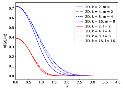
Figure 1: $n_{\beta}^{2}({\bf x})/\omega_{\text{tr}}^{d}$ as a function of the radial coordinate $\rho$, for several cutoff values of the quantum numbers $k,m$ in 2D (blue) and $k,l$ in 3D (red); in the latter case, the quantum number $m$ is summed over its full range $[-l,l]$. In this plot, $\omega_{z}/\omega_{\text{tr}}=1/2$.

Thus, in 2D,

$$n_{\beta}({\bf x})=\omega_{\text{tr}}\frac{e^{-\rho^{2}}}{2\pi}\sum_{k,m}e^{-\beta E_{km}}f^{\text{2D}}_{km}(\rho^{2}),$$ (38)

whose units come from the prefactor $\omega_{\text{tr}}$ and, as expected from symmetry considerations, is only a function of the radial coordinate (concentric with the trapping potential). Here,

$$f^{\text{2D}}_{km}(\rho^{2})\equiv\frac{2\,k!}{(k+|m|)!}\rho^{2|m|}\left(L_{k}^{|m|}(\rho^{2})\right)^{2},$$ (39)

Similarly, in 3D,

$$n_{\beta}({\bf x})=\omega_{\text{tr}}^{3/2}\frac{e^{-\rho^{2}}}{\sqrt{4\pi}}\sum_{k,l,m}e^{-\beta E_{klm}}f^{\text{3D}}_{kl}(\rho^{2})(P^{m}_{l}(\cos\theta))^{2}$$ (40)

where

$$f^{\text{3D}}_{kl}(\rho^{2})\equiv\frac{2^{k+2l+3}\,k!}{(2k+2l+1)!!}\rho^{2l}\left(L_{k}^{l+1/2}(\rho^{2})\right)^{2}$$ (41)

Using the above results, together with Eq. (16) for $\Delta b_{2}$, we solve for the dimensionless quantity $B/\lambda_{T}^{d}$ in terms of $\Delta b_{2}$:

$$\frac{C}{\lambda_{T}^{d}}=\Delta b_{2}\frac{Q_{1}}{(2\pi\beta\omega_{\text{tr}})^{d/2}}\left({\int d^{d}{\bf\bar{x}}\;\,\frac{n_{\beta}^{2}({\bf\bar{x}})}{\omega_{\text{tr}}^{d}}}\right)^{-1}.$$ (42)

II.3.2 Three-body sector: $\Delta Q_{2,1}$ for fermions

Following the same steps outlined above, it is straightforward to show that

$$\Delta Q_{2,1} = \frac{C}{2}\sum_{{\bf k}_{1}{\bf k}_{2}{\bf k}_{3}}e^{-\beta(E_{{\bf k}_{1}}+E_{{\bf k}_{2}}+E_{{\bf k}_{3}})}$$ (43)

$$\ \ \times\sum_{{\bf x}_{1}{\bf x}_{2}}|\langle{\bf x}_{1}{\bf x}_{2}{\bf x}_{1}|{\bf k}_{1}{\bf k}_{2}{\bf k}_{3}\rangle|^{2}.$$

The overlap can be simplified slightly by factoring across distinguishable species:

$$\langle{\bf x}_{1}{\bf x}_{2}{\bf x}_{1}|{\bf k}_{1}{\bf k}_{2}{\bf k}_{3}\rangle = \langle{\bf x}_{1}{\bf x}_{2}|{\bf k}_{1}{\bf k}_{2}\rangle\langle{\bf x}_{1}|{\bf k}_{3}\rangle,$$ (44)

where the matrix element $\langle{\bf x}_{1}{\bf x}_{2}|{\bf k}_{1}{\bf k}_{2}\rangle$ is a Slater determinant of single-particle states:

$$\langle{\bf x}_{1}{\bf x}_{2}|{\bf k}_{1}{\bf k}_{2}\rangle=\langle{\bf x}_{1}|{\bf k}_{1}\rangle\langle{\bf x}_{2}|{\bf k}_{2}\rangle-\langle{\bf x}_{2}|{\bf k}_{1}\rangle\langle{\bf x}_{1}|{\bf k}_{2}\rangle.$$ (45)

As in the case of $\Delta Q_{1,1}$, we will sum over the energy eigenstates first, and then perform the spatial sum. To that end, it is useful to define

$$n^{F}_{\beta}({\bf x}_{1},{\bf x}_{2})=n_{\beta}({\bf x}_{1})\sum_{{\bf k}_{1}{\bf k}_{2}}e^{-\beta(E_{{\bf k}_{1}}+E_{{\bf k}_{2}})}|\langle{\bf x}_{1}{\bf x}_{2}|{\bf k}_{1}{\bf k}_{2}\rangle|^{2},$$ (46)

such that,

$$\Delta Q_{2,1} = \frac{C}{2}\sum_{{\bf x}_{1}{\bf x}_{2}}n^{F}_{\beta}({\bf x}_{1},{\bf x}_{2}).$$ (47)

As in the case of $n_{\beta}({\bf x})$, the exponential decay with the energy allows us to cutoff the double sum in $n^{F}_{\beta}({\bf x}_{1},{\bf x}_{2})$ without significantly affecting the precision of the whole calculation.

II.3.3 Three-body sector: $\Delta Q_{2,1}$ for bosons

The bosonic case differs from the fermionic case in that we must use a permanent rather than a Slater determinant. Thus,

$$n^{B}_{\beta}({\bf x}_{1},{\bf x}_{2})=n_{\beta}({\bf x}_{1})\sum_{{\bf k}_{1}{\bf k}_{2}}e^{-\beta(E_{{\bf k}_{1}}+E_{{\bf k}_{2}})}|\langle{\bf x}_{1}{\bf x}_{2}|{\bf k}_{1}{\bf k}_{2}\rangle|^{2},$$ (48)

where the two-body overlap is now symmetric in its arguments, as befits bosons:

$$\langle{\bf x}_{1}{\bf x}_{2}|{\bf k}_{1}{\bf k}_{2}\rangle=\langle{\bf x}_{1}|{\bf k}_{1}\rangle\langle{\bf x}_{2}|{\bf k}_{2}\rangle+\langle{\bf x}_{2}|{\bf k}_{1}\rangle\langle{\bf x}_{1}|{\bf k}_{2}\rangle.$$ (49)

II.3.4 Gaussian quadrature

As shown above, the single-particle wavefunctions [c.f. Eqs. (20) and (26)] and the associated density functions $n_{\beta}({\bf x})$, $n^{F,B}_{\beta}({\bf x}_{1},{\bf x}_{2})$, are governed in the radial variable by a Gaussian decay. For that reason, it is appropriate to calculate the corresponding integrals using Gauss-Hermite quadrature. The corresponding $M$ points $x_{i}$ and $M$ weights $w_{i}$ allow us to estimate integrals according to

$$\int_{-\infty}^{\infty}dx\,e^{-x^{2}}f(x)=\sum_{i=0}^{M-1}w_{i}f(x_{i}).$$ (50)

In this work we use the same quadrature points and weights as in our previous work of Refs. Casey1 ; Casey2 ; Casey3 .

III Results

III.1 Noninteracting virial coefficients at finite angular momentum

For future reference, and because we have not been able to locate these results elsewhere in the literature, we present here the calculation of the noninteracting virial expansion when $\omega_{z}\neq 0$. We begin with the well-known result for the partition function of spin-$1/2$ fermions in terms of the single-particle energies $E$:

$$\ln\mathcal{Z}=2\sum_{E}\ln\left(1+ze^{-\beta E}\right),$$ (51)

which is valid for arbitrary positive $z$, whereas for (doubly degenerate) bosons

$$\ln\mathcal{Z}=2\sum_{E}\ln\left(\frac{1}{1-ze^{-\beta E}}\right),$$ (52)

which is valid for arbitrary $z<\exp(\beta E_{0})$, where $E_{0}$ is the ground-state energy [$z=\exp(\beta E_{0})$ being the well-known limit of Bose-Einstein condensation]. From these expressions, it is easy to see that the virial coefficients $b_{n}$ for noninteracting bosons and fermions differ by a factor of $(-1)^{n+1}$. As is well known, for homogeneous, nonrelativistic fermions in $d$ dimensions, $b_{n}=(-1)^{n+1}n^{-(d+2)/2}$. Below, we address the generalization of this formula to harmonically trapped systems at finite angular momentum in 2D and 3D.

III.1.1 Two spatial dimensions

In 2D, $E=E_{km}=\omega_{\text{tr}}(2k+|m|+1)+\omega_{z}m$, where $k\geq 0$ and $m$ is summed over all integers. Thus, we may write the sum by Taylor-expanding the logarithm as

$$\ln\mathcal{Z} = 2\sum_{n=1}^{\infty}\frac{(-1)^{n+1}}{n}{z^{n}e^{-n\beta\omega_{\text{tr}}}}\sum_{k=0}^{\infty}e^{-\beta\omega_{\text{tr}}2kn}\times$$ (53)

$$\left[\sum_{m=0}^{\infty}e^{-\beta\omega_{+}mn}+\sum_{\bar{m}=1}^{\infty}e^{-\beta\omega_{-}\bar{m}n}\right].$$

where $\omega_{\pm}=\omega_{\text{tr}}\pm\omega_{z}$. Carrying out the sums over $k,m,\bar{m}$, we obtain

$$\ln\mathcal{Z}=Q_{1}\sum_{n=1}^{\infty}b_{n}z^{n},$$ (54)

where

$$Q_{1}b_{n}=\frac{2\,(-1)^{n+1}}{n}\frac{e^{-n\beta\omega_{\text{tr}}}}{(1-e^{-n\beta\omega_{+}})(1-e^{-n\beta\omega_{-}})}.$$ (55)

Finally, to determine $b_{n}$ we use $Q_{1}$ as derived above in Eqs. (25) and (30), such that

$$b_{n} = \frac{(-1)^{n+1}}{n}e^{-\beta\omega_{\text{tr}}(n-1)}\frac{(1\!-\!e^{-\beta\omega_{+}})(1\!-\!e^{-\beta\omega_{-}})}{(1\!-\!e^{-n\beta\omega_{+}})(1\!-\!e^{-n\beta\omega_{-}})}.$$ (56)

Note that the $b_{n}$ are always finite, in particular in the ‘deconfinement limit’ referred to in the introduction where $\omega_{-}\to 0$,

$$b_{n}\to b_{n}^{\text{DL2D}}\equiv\frac{(-1)^{n+1}}{n^{2}}e^{-\beta\omega_{\text{tr}}(n-1)}\frac{(1-e^{-2\beta\omega_{\text{tr}}})}{(1-e^{-2n\beta\omega_{\text{tr}}})}.$$ (57)

On the other hand, $Q_{1}$ diverges in that limit, because the energy spectrum then becomes independent from $m$. Simply put, in that limit the centrifugal motion due to rotation is strong enough to overcome the trapping potential and the system escapes to infinity. In terms of $\ln\mathcal{Z}$, the divergence may be regarded as a phase transition at $\omega_{z}=\omega_{\text{tr}}$. Below we further interpret this limit, considering the 2D and 3D cases simultaneously.

We can now derive a virial expansion for the angular momentum and the $z$ component of the moment of inertia:

$$\langle\hat{L}_{z}\rangle=\frac{\partial\ln\mathcal{Z}}{\partial(\beta\omega_{z})}=Q_{1}\sum_{n=1}^{\infty}L_{n}z^{n},$$ (58)

where

$$L_{n}=\frac{1}{Q_{1}}\frac{\partial\left(Q_{1}b_{n}\right)}{\partial(\beta\omega_{z})}=nb_{n}\frac{e^{-n\beta\omega_{-}}-e^{-n\beta\omega_{+}}}{(1-e^{-n\beta\omega_{+}})(1-e^{-n\beta\omega_{-}})},$$ (59)

and

$$I_{z}=\frac{\partial^{2}\ln\mathcal{Z}}{\partial(\beta\omega_{z})^{2}}=Q_{1}\sum_{n=1}^{\infty}I_{n}z^{n},$$ (60)

where

$$I_{n} = \frac{1}{Q_{1}}\frac{\partial(Q_{1}L_{n})}{\partial(\beta\omega_{z})}$$

$$= \!\!-nL_{n}\!\!\left[\frac{e^{-n\beta\omega_{+}}\!+\!e^{-n\beta\omega_{-}}}{e^{-n\beta\omega_{+}}\!-\!e^{-n\beta\omega_{-}}}\!+\!\frac{2(e^{-n\beta\omega_{+}}\!-\!e^{-n\beta\omega_{-}})}{(1\!-\!e^{-n\beta\omega_{+}})(1\!-\!e^{-n\beta\omega_{-}})}\right].$$

Note that, correctly, $L_{n}\to 0$ at $\omega_{+}=\omega_{-}$, which corresponds to $\omega_{z}=0$, i.e. no rotation. On the other hand, as may be expected from our previous discussion $L_{n}\to\infty$ as $\omega_{-}\to 0$, as in that limit the induced rotation overpowers the external potential that holds the system together. Furthermore, at $\omega_{z}=0$, a finite moment of inertia remains:

$$I_{n}\to 2n(-1)^{n+1}e^{-(2n-1)\beta\omega_{\text{tr}}}\frac{(1-e^{-\beta\omega_{\text{tr}}})^{2}}{(1-e^{-n\beta\omega_{\text{tr}}})^{4}},$$ (62)

which characterizes the static response to small rotation frequencies within the virial expansion, as a function of $\beta\omega_{\text{tr}}$.

III.1.2 Three spatial dimensions

In 3D, $E=E_{klm}=\omega_{\text{tr}}(2k+l+3/2)+\omega_{z}m$, where $k\geq 0$, $l\geq 0$, and $-l\leq m\leq l$. Therefore, analyzing the problem as in the 2D case, we obtain

$$Q_{1}b_{n}=\frac{2\,(-1)^{n+1}}{n}\frac{e^{-\frac{3}{2}n\beta\omega_{\text{tr}}}}{(1\!-\!e^{-n\beta\omega_{\text{tr}}})(1\!-\!e^{-n\beta\omega_{+}})(1\!-\!e^{-n\beta\omega_{-}})},$$ (63)

and

$$b_{n} = \frac{(-1)^{n+1}}{n}e^{-\frac{3}{2}\beta\omega_{\text{tr}}(n-1)}\times$$ (64)

$$\frac{(1-e^{-\beta\omega_{\text{tr}}})(1-e^{-\beta\omega_{+}})(1-e^{-\beta\omega_{-}})}{(1-e^{-n\beta\omega_{\text{tr}}})(1-e^{-n\beta\omega_{+}})(1-e^{-n\beta\omega_{-}})}.$$

As in the 2D case, the $b_{n}$ are always finite and, in particular in the deconfinement limit $\omega_{-}\to 0$,

$$b_{n}\to b_{n}^{\text{DL3D}} \equiv \frac{(-1)^{n+1}}{n^{2}}e^{-\frac{3}{2}\beta\omega_{\text{tr}}(n-1)}$$ (65)

$$\times\frac{(1-e^{-\beta\omega_{\text{tr}}})}{(1-e^{-n\beta\omega_{\text{tr}}})}\frac{(1-e^{-2\beta\omega_{\text{tr}}})}{(1-e^{-2n\beta\omega_{\text{tr}}})},$$

whereas $Q_{1}$ diverges in that limit. In this case, the problem can be traced back to the infinite sequence of states for which $\ell=-m$. We can also obtain expressions for the virial expansion of the angular momentum and the moment of inertia. Because the dependence of $Q_{1}b_{n}$ on $\omega_{+}$ and $\omega_{-}$ is the same in 2D and 3D, the relationship between $L_{n}$ and $b_{n}$ is identical in 2D and 3D, i.e. Eq. (59) is valid in 3D, as long as the $b_{n}$ corresponding to 3D is used in the right-hand side. Similarly, Eq. (III.1.1) for $I_{n}$ carries over to 3D, as long as the $L_{n}$ corresponding to 3D is used in the right-hand side. As expected, and as in the 2D case, $L_{n}\to 0$ at $\omega_{z}=0$, whereas

$$I_{n}\to 2n(-1)^{n+1}e^{-\frac{1}{2}\beta\omega_{\text{tr}}(5n-3)}\frac{(1-e^{-\beta\omega_{\text{tr}}})^{3}}{(1-e^{-n\beta\omega_{\text{tr}}})^{5}}.$$ (66)

The impact of rotation, i.e. a finite $\beta\omega_{z}$ on a noninteracting system is displayed in Fig. 2, where we show the ratio of the rotating to non-rotating virial coefficients. This ratio is the same for bosons and fermions in the noninteracting case and it drastically increases as $\omega_{z}$ approaches $\omega_{\text{tr}}$. At large $n$, this ratio becomes

$$\frac{b_{n}}{b_{n}(\beta\omega_{z}=0)}\to\frac{(1-e^{-\beta\omega_{+}})(1-e^{-\beta\omega_{-}})}{(1-e^{-\beta\omega_{\text{tr}}})^{2}}.$$ (67)

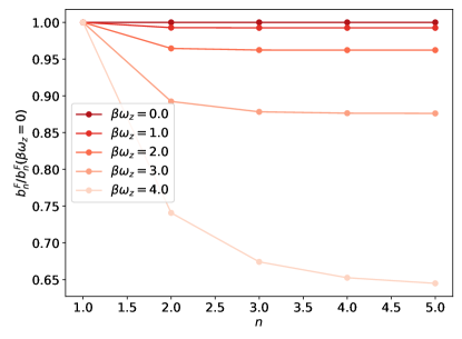
Figure 2: Noninteracting $b_{n}$ normalized by their non-rotating, noninteracting values $b_{n}(\beta\omega_{z}=0)$, as functions of $n$ for a few values of $\beta\omega_{z}$ and fixed $\beta\omega_{\text{tr}}=5$. The ratio $b_{n}/b_{n}(\beta\omega_{z}=0)$ is the same for bosons and fermions, and is the same in 2D and 3D.

Naturally, the total angular momentum will increase with $\omega_{z}$. For a noninteracting system the result is shown in Fig. 3 as a function of $\omega_{z}/\omega_{\text{tr}}$, at several temperatures $\beta\omega_{\text{tr}}$. At small $\omega_{z}$, we find the linear response regime from which we can extract the moment of inertia $I_{z}$, as shown in Fig. 4. At the lowest temperatures (highest values of $\beta\omega_{\text{tr}}$), the response of the system to rotation is highly suppressed, as seen in both Fig. 3 and Fig. 4. On the other hand, at high temperatures (low $\beta\omega_{\text{tr}}$), where response is higher, we find a mild non-linear regime in which $I_{z}$ varies as a function of $\omega_{z}/\omega_{\text{tr}}$.

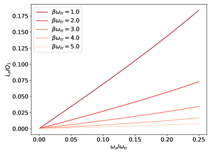
Figure 3: Noninteracting $L_{z}/Q_{1}$ in for bosons in 3D, as a function of $\omega_{z}/\omega_{\text{tr}}$ for a few different temperatures $\beta\omega_{\text{tr}}$, at third order in the virial expansion.

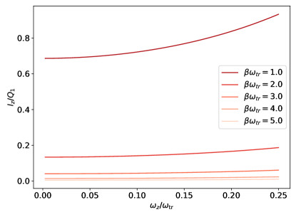
Figure 4: Noninteracting $I_{z}/Q_{1}$ in for bosons in 3D, as a function of $\omega_{z}/\omega_{\text{tr}}$ for a few different temperatures $\beta\omega_{\text{tr}}$, at third order in the virial expansion.

III.1.3 The virial expansion in the deconfinement limit

Using the limiting expressions for the trapped, rotating $b_{n}$ in 2D and 3D, namely Eqs. (57) and (65), respectively, we may analyze the behavior of the system in that limit. To that end, we analyze those equations isolating their asymptotic form, which dominates the behavior of the virial expansion series:

$$b_{n}^{\text{DL2D}}\simeq 2\frac{(-1)^{n+1}}{n^{2}}e^{-\beta\omega_{\text{tr}}n}\sinh(\beta\omega_{\text{tr}}),$$ (68)

$$b_{n}^{\text{DL3D}}\simeq 4\frac{(-1)^{n+1}}{n^{2}}e^{-\frac{3}{2}\beta\omega_{\text{tr}}n}\sinh(\beta\omega_{\text{tr}}/2)\sinh(\beta\omega_{\text{tr}}),$$ (69)

We thus see that the thermodynamics of the deconfined limit is governed in 2D by

$$\frac{\ln\mathcal{Z}}{Q_{1}}\simeq-2\sinh(\beta\omega_{\text{tr}})\;\text{Li}_{2}(-e^{-\beta\omega_{\text{tr}}}z),$$ (70)

where $\text{Li}_{n}(x)$ is the polylogarithm function of order $n$. Similarly, in 3D we obtain

$$\frac{\ln\mathcal{Z}}{Q_{1}}\simeq-4\sinh(\beta\omega_{\text{tr}}/2)\sinh(\beta\omega_{\text{tr}})\;\text{Li}_{2}(-e^{-\frac{3}{2}\beta\omega_{\text{tr}}}z).$$ (71)

Notably, and prefactors aside, both the 2D and 3D cases are completely captured by the same polylogarithm function. More specifically, $\text{Li}_{2}(x)$ is the same function that characterizes the 2D homogeneous quantum gas (both fermions and bosons). We therefore see explicitly how, in the deconfined limit, the maximized angular momentum flattens the (3D) system and effectively turns it into a homogeneous 2D gas, with a shifted chemical potential. While above we have written the results for fermions, analogous expressions are valid for bosons.

III.2 Interaction effects on the virial expansion

In this section we use our results for $\Delta b_{2}$ and $\Delta b_{3}$ to calculate the angular momentum equation of state, as well as the static response encoded in the moment of inertia. Denoting the noninteracting grand canonical partition function by $\mathcal{Z}_{0}$, we have

$$\ln\left(\mathcal{Z}/\mathcal{Z}_{0}\right)=Q_{1}\sum_{n=2}^{\infty}\Delta b_{n}z^{n},$$ (72)

such that the interaction effect on the angular momentum virial coefficient $L_{n}$ is

$$\Delta L_{n}=\frac{1}{Q_{1}}\frac{\partial\left(Q_{1}\Delta b_{n}\right)}{\partial(\beta\omega_{z})}=\frac{\partial\left(\Delta b_{n}\right)}{\partial(\beta\omega_{z})}+\Delta b_{n}\frac{\partial\left(\ln Q_{1}\right)}{\partial(\beta\omega_{z})},$$ (73)

and its counterpart for the moment of inertia is

$$\Delta I_{n}=\frac{1}{Q_{1}}\frac{\partial\left(Q_{1}\Delta L_{n}\right)}{\partial(\beta\omega_{z})}=\frac{\partial\left(\Delta L_{n}\right)}{\partial(\beta\omega_{z})}+\Delta L_{n}\frac{\partial\left(\ln Q_{1}\right)}{\partial(\beta\omega_{z})},$$ (74)

where, using the previous equation for $\Delta L_{n}$,

$$\frac{\partial\left(\Delta L_{n}\right)}{\partial(\beta\omega_{z})}=\frac{\partial^{2}\left(\Delta b_{n}\right)}{\partial(\beta\omega_{z})^{2}}+\frac{\partial\left(\Delta b_{n}\right)}{\partial(\beta\omega_{z})}\frac{\partial\left(\ln Q_{1}\right)}{\partial(\beta\omega_{z})}+\Delta b_{n}\frac{\partial^{2}\left(\ln Q_{1}\right)}{\partial(\beta\omega_{z})^{2}}.$$ (75)

Using the above formulas, along with the expressions obtained above for $\Delta b_{2}$ and $\Delta b_{3}$ in the coarse temporal lattice approximation, we readily obtain expressions for the interaction-induced change in the second- and third-order virial coefficients for the angular momentum and moment of inertia, namely $\Delta L_{2}$, $\Delta L_{3}$, $\Delta I_{2}$, and $\Delta I_{3}$. Based on those, we can rebuild $\langle\hat{L}_{z}\rangle/Q_{1}$ and $I_{z}/Q_{1}$ and explore their change due to interactions in the virial region, which we show for fermions in Figs. 5 and 6. In both figures we find that interactions change the response to rotation: both the angular momentum and the moment of inertia are modified by correlations, and the effect increases with $\omega_{z}$. In particular, attractive interactions tend to make the system more compact (i.e. they reduce the size of the cloud) thus reducing the moment of inertia and the total angular momentum, for a given rotational frequency. The corresponding opposite behavior is found for repulsive interactions.

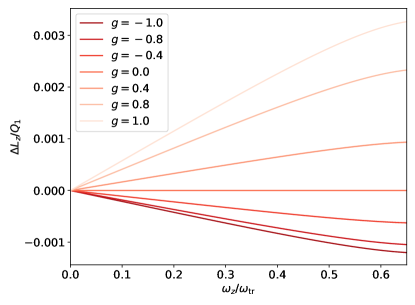
Figure 5: Interaction-induced change in the angular momentum of a 3D Fermi gas with attractive and repulsive contact interactions, as a function of the rotation frequency $\omega_{z}$ in units of the trapping frequency $\omega_{\text{tr}}$, at $z=\exp(-2.0)$.

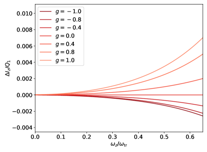
Figure 6: Interaction-induced change in the moment of inertia of a 3D Fermi gas with attractive and repulsive contact interactions, as a function of the rotation frequency $\omega_{z}$ in units of the trapping frequency $\omega_{\text{tr}}$, at $z=\exp(-2.0)$.

IV Summary and Conclusions

In this work, we have characterized the thermodynamics of rotating Bose and Fermi gases in 2D and 3D using the virial expansion. To that end, we calculated the effect of rotation on the virial coefficients $b_{n}$ corresponding to the pressure and density equations of state, as well as on the virial coefficients for the angular momentum $L_{n}$ and moment of inertia $I_{n}$. We carried out calculations for interacting as well as noninteracting systems.

In the absence of interactions, we obtained analytic formulas for $b_{n}$, $L_{n}$, and $I_{n}$ in 2D and 3D, which were absent from the literature to the best of our knowledge. We noted that, while the $b_{n}$ remain finite when $\omega_{z}$ approaches $\omega_{\text{tr}}$, the $L_{n}$, and $I_{n}$ coefficients diverge, as does the single-particle partition function $Q_{1}$. The origin of the divergence is traced back to the fact that the system becomes unstable at $\omega_{z}=\omega_{\text{tr}}$; in that deconfinement limit, the high angular velocity enables particles to escape the trapping potential. By exploring the asymptotic behavior of $b_{n}$ in that limit, we found that (up to overall factors) it corresponds to that of a homogeneous 2D gas with a chemical potential shifted by the zero-point energy of the trapping potential.

To address the interacting cases, we implemented a coarse temporal lattice approximation, which allowed us to bypass solving the rotating $n$-body problem to calculate the $n$-th order virial coefficient, which we accessed at second and third orders. Based on those results, we obtained qualitative estimates for the angular momentum as well as the moment of inertia, as functions of the angular velocity $0<\omega_{z}<\omega_{\text{tr}}$ and temperature $\beta\omega_{\text{tr}}$. Notably, we find that both the interacting and noninteracting cases display linear response to rotation at low $\omega_{z}$, as expected, but we are also able to distinguish a non-linear regime in which $I_{z}$ varies with $\omega_{z}$; this is most evident at high temperatures and above $\omega_{z}/\omega_{\text{tr}}\simeq 0.1$.

Our work represents a step toward characterizing the properties of rotating matter in high-temperature regimes. Future studies using increased computational power should be able to explore higher-order corrections to the coarse lattice approximation presented here.

This material is based upon work supported by the National Science Foundation under Grant No. PHY1452635 (Computational Physics Program). C.E.B. acknowledges support from the United States Department of Energy through the Computational Science Graduate Fellowship (DOE CSGF) under grant number DE-FG02-97ER25308.

Appendix A Single-particle basis in 2D

For completeness, in this appendix we show the solution of the Schrödinger equation for a harmonically trapped particle coupled to the $z$ component of angular momentum in 2D. The purpose of presenting this information is to establish our notation and to provide a reference point for future work.

We begin with the Schrödinger equation in polar coordinates:

$$\left(-\frac{\partial^{2}}{\partial r^{2}}-\frac{1}{r}\frac{\partial}{\partial r}-\frac{1}{r^{2}}\frac{\partial^{2}}{\partial\phi^{2}}+m^{2}\omega_{\text{tr}}^{2}r^{2}-2mE\right)\Psi(r,\phi) = 0$$

We then change variables such that $\rho=m\sqrt{\omega_{\text{tr}}}r$, and $m,\hbar=1$, which yields

$$r \to \frac{1}{\sqrt{\omega_{\text{tr}}}}\rho,$$

$$\frac{\partial}{\partial r} \to \sqrt{\omega_{\text{tr}}}\frac{\partial}{\partial\rho},$$

$$\frac{\partial^{2}}{\partial r^{2}} \to \omega_{\text{tr}}\frac{\partial^{2}}{\partial\rho^{2}}.$$

With those replacements, we write $\Psi(\rho,\phi)$ as a product of functions of two individual variables, $\Psi(\rho,\phi)=R(\rho)\Phi(\phi)$, such that

$$\left[-\left(\rho^{2}\frac{\partial^{2}}{\partial\rho^{2}}+\rho\frac{\partial}{\partial\rho}+\frac{\partial^{2}}{\partial\phi^{2}}\right)+\rho^{4}-2\rho^{2}\frac{E}{\omega_{\text{tr}}}\right]R(\rho)\Phi(\phi)=0,$$

This decouples our partial differential equation into two ordinary equations, each of which must be equal to a constant $\widetilde{m}^{2}$:

$$-\frac{1}{\Phi(\phi)}\frac{\partial^{2}}{\partial\phi^{2}}\Phi(\phi)=\widetilde{m}^{2},$$

$$-\frac{\rho^{2}}{R(\rho)}\frac{\partial^{2}R(\rho)}{\partial\rho^{2}}-\frac{\rho}{R(\rho)}\frac{\partial R(\rho)}{\partial\rho}+\rho^{4}-2\rho^{2}\frac{E}{\omega_{\text{tr}}}=-\widetilde{m}^{2}.$$

We can solve the equation for $\Phi(\phi)$ straightforwardly: $\Phi(\phi)\propto e^{i\widetilde{m}\phi}$, with the constraint that $\widetilde{m}$ must be an integer to ensure the solution is not multivalued.

The equation for $\rho$, setting $\widetilde{E}={E}/{\omega_{\text{tr}}}$, is then

$$-\rho^{2}\frac{\partial^{2}R(\rho)}{\partial\rho^{2}}-\rho\frac{\partial R(\rho)}{\partial\rho}+\left(\widetilde{m}^{2}+\rho^{4}-2\rho^{2}\widetilde{E}\right)R(\rho)=0.$$ (76)

At long distances ($\rho\rightarrow\infty$) we have a harmonic oscillator equation

$$-\frac{\partial^{2}R(\rho)}{\partial\rho^{2}}+\rho^{2}R(\rho)=2\widetilde{E}R(\rho),$$ (77)

which indicates that at long distances the solution behaves as a Gaussian.

At short distances ($\rho\ll 1$), on the other hand, our equation reduces to

$$-\rho^{2}\frac{\partial^{2}R(\rho)}{\partial\rho^{2}}-\rho\frac{\partial R(\rho)}{\partial\rho}+\widetilde{m}^{2}R(\rho)=0.$$ (78)

We can approach this by proposing proposing $R(\rho)=R_{0}\rho^{c}$, which leads to an equation for the power $c$ in terms of our constant $\widetilde{m}$:

$$-c^{2}=\widetilde{m}^{2},\ c=\pm\widetilde{m}.$$ (79)

The case $\widetilde{m}=0$ yields two solutions: a constant $R(\rho)=R_{0}$ and $R(\rho)=\ln\rho$. We can discard the second one since it diverges at the origin, which our wave function should not do. For the same reason we discard the case $\widetilde{m}<0$. Therefore, the short-distance behavior is $R(\rho)\propto\rho^{|\widetilde{m}|}$.

Based on the above analysis, we propose for the full solution the form:

$$R(\rho)=e^{-\rho^{2}/2}\rho^{|\widetilde{m}|}F(\rho),$$ (80)

where $F(\rho)$ is a function to be determined. This captures the behavior of $R(\rho)$ in our limiting cases. With that form, the radial equation becomes

$$\rho^{2}\frac{\partial^{2}F(\rho)}{\partial\rho^{2}}+\frac{\partial F(\rho)}{\partial\rho}(b_{\widetilde{m}}\rho-2\rho^{3})-2a_{\widetilde{m}}\rho^{2}F(\rho)=0,$$ (81)

where $a_{\widetilde{m}}\equiv 1-\widetilde{E}+|\widetilde{m}|$ and $b_{\widetilde{m}}\equiv 2|\widetilde{m}|+1$. We propose a power series form

$$F(\rho)=\sum_{k=0}^{\infty}\rho^{k}c_{k}$$ (82)

and obtain algebraic equations for $c_{k}$ from Eq. (81). Analyzing the lowest powers we obtain the following conditions: From the lowest two powers of $\rho$, we find that $c_{0}$ is not fixed but that $c_{1}=0$. The remaining coefficients are related by the recursion

$$c_{k+2}=\frac{2(k+a_{\widetilde{m}})}{(k+2)(k+1+b_{\widetilde{m}})}c_{k}$$ (83)

Thus, if both $c_{0}$ and $c_{1}$ vanish, then the solution vanishes identically. On the other hand, setting $c_{0}=1$, only the odd coefficients vanish and we obtain the remaining coefficients recursively. The overall normalization can be set after the fact since the equation is linear. The series terminates if $k=a_{\widetilde{m}}$ for some $k=2n\geq 0$ (recall only the even $k$ survive), which yields the quantization condition:

$$\frac{E}{\omega_{\text{tr}}} = 2n+|\widetilde{m}|+1.$$ (84)

References

- (1) S. Giorgini, L.P. Pitaevskii, S. Stringari, Theory of ultracold Fermi gases, Rev. Mod. Phys. 80, 1215 (2008).
- (2) I. Bloch, J. Dalibard, W. Zwerger Many-Body Physics with Ultracold Gases, Rev. Mod. Phys. 80, 885 (2008).
- (3) M. Lewenstein, A. Sanpera, V. Ahufinger, Ultracold Atoms in Optical Lattices: Simulating Quantum Many-body Systems, (Oxford University Press, New York, 2012)
- (4) C. Chin, R. Grimm, P. Julienne, and E. Tiesinga, Feshbach resonances in ultracold gases, Rev. Mod. Phys. 82, 1225 (2010).
- (5) F. Chevy and C. Mora, Ultra-cold polarized Fermi gases, Rep. Prog. Phys. 73, 112401 (2010)
- (6) Ultracold Fermi Gases, Proceedings of the International School of Physics “Enrico Fermi”, Course CLXIV, Varenna, June 20 – 30, 2006, M. Inguscio, W. Ketterle, C. Salomon (Eds.) (IOS Press, Amsterdam, 2008).
- (7) M. H. Anderson, J. R. Ensher, M. R. Matthews, C. E. Wieman, E. A. Cornell, Observation of Bose-Einstein Condensation in a Dilute Atomic Vapor, Science 269, 198 (1995).
- (8) Davis, K. B. and Mewes, M. -O. and Andrews, M. R. and van Druten, N. J. and Durfee, D. S. and Kurn, D. M. and Ketterle, W., Bose-Einstein Condensation in a Gas of Sodium Atoms, Phys. Rev. Lett. 75, 3969 (1995)
- (9) Regal, C. A. and Greiner, M. and Jin, D. S., Observation of Resonance Condensation of Fermionic Atom Pairs, Phys. Rev. Lett. 92, 040403 (2004).
- (10) Zwierlein, M. W. and Stan, C. A. and Schunck, C. H. and Raupach, S. M. F. and Kerman, A. J. and Ketterle, W., Condensation of Pairs of Fermionic Atoms near a Feshbach Resonance, Phys. Rev. Lett. 92, 120403 (2004).
- (11) Matthews, M. R., B. P. Anderson, P. C. Haljan, D. S. Hall, M. J. Holland, J. E. Williams, C. E. Wieman, and E. A. Cornell, Watching a Superfluid Untwist Itself: Recurrence of Rabi Oscillations in a Bose-Einstein Condensate, Phys. Rev. Lett. 83, 3358 (1999).
- (12) Madison, K. W., F. Chevy, W. Wohlleben, and J. Dalibard, Vortex Formation in a Stirred Bose-Einstein Condensate, Phys. Rev. Lett. 84, 806 (2000).
- (13) M.W. Zwierlein, J.R. Abo-Shaeer, A. Schirotzek, C.H. Schunck, W. Ketterle, Vortices and Superfluidity in a Strongly Interacting Fermi Gas, Nature 435, 1047-1051 (2005).
- (14) N. Cooper, Rapidly rotating atomic gases, Advances in Physics, 57, 539 (2008).
- (15) A. L. Fetter, Rotating trapped Bose-Einstein condensates, Rev. Mod. Phys. 81, 647 (2009).
- (16) S. Stringari Phase Diagram of Quantized Vortices in a Trapped Bose-Einstein Condensed Gas, Phys. Rev. Lett. 82, 4371 (1999).
- (17) X.-J. Liu, Virial expansion for a strongly correlated Fermi system and its application to ultracold atomic Fermi gases, Phys. Rep. 524, 37 (2013).
- (18) E. Beth and G. E. Uhlenbeck, The quantum theory of the non-ideal gas. II. Behaviour at low temperatures, Physica (Utrecht) 4, 915 (1937).
- (19) X.J. Liu, H. Hu, and P. D. Drummond Exact few-body results for strongly correlated quantum gases in two dimensions, Phys. Rev. B 82, 054524 (2010).
- (20) T. Busch, B.-G. Englert, K. Rza̧żewski, and M. Wilkens, Foundations of Physics 28, 549 (1998).
- (21) C. R. Shill, J. E. Drut, Virial coefficients of 1D and 2D Fermi gases by stochastic methods and a semiclassical lattice approximation, Phys. Rev. A 98, 053615 (2018).
- (22) Y. Hou, A. Czejdo, J. DeChant, C. R. Shill, J. E. Drut, Leading-order semiclassical approximation to the first seven virial coefficients of spin-1/2 fermions across spatial dimensions, Phys. Rev. A 100, 063627 (2019).
- (23) K. J. Morrell, C. E. Berger, and J. E. Drut, Third- and fourth-order virial coefficients of harmonically trapped fermions in a semiclassical approximation, Phys. Rev. A 100, 063626 (2019).
- (24) B. C. Mulkerin, C. J. Bradly, H. M. Quiney, and A. M. Martin, Universality in rotating strongly interacting gases, Phys. Rev. A 85, 053636 (2012).
- (25) B. C. Mulkerin, C. J. Bradly, H. M. Quiney, and A. M. Martin, Universality and itinerant ferromagnetism in rotating strongly interacting Fermi gases, Phys. Rev. A 86, 053631 (2012)
- (26) Y. Li, Rotating ideal Fermi gases under a harmonic potential, Physica B 481, 38 (2016).
- (27) Y. Li and Q. Gu The particle flow oscillations of rotating non-interacting gases in a two-dimensional harmonic trap, Phys. Lett. A 380, 353 (2016).
- (28) Y. Hou, J. E. Drut, Semiclassical approximation to virial coefficients beyond the leading order, arXiv:1908.00174.
- (29) C. E. Berger, E. R. Anderson, and J. E. Drut, Energy, contact, and density profiles of one-dimensional fermions in a harmonic trap via nonuniform-lattice Monte Carlo calculations, Phys. Rev. A 91, 053618 (2015).
- (30) C. E. Berger, J. E. Drut, and W. J. Porter, Hard-wall and non-uniform lattice Monte Carlo approaches to one-dimensional Fermi gases in a harmonic trap, Comput. Phys. Commun. 208, 103 (2016).
- (31) Z. Luo, C. E. Berger, and J. E. Drut, Harmonically trapped fermions in two dimensions: Ground-state energy and contact of SU(2) and SU(4) systems via a nonuniform lattice Monte Carlo method, Phys. Rev. A 93, 033604 (2016).