Precision angular diameters for 16 southern stars with VLTI/PIONIER

Abstract

In the current era of Gaia and large, high signal to noise stellar spectroscopic surveys, there is an unmet need for a reliable library of fundamentally calibrated stellar effective temperatures based on accurate stellar diameters. Here we present a set of precision diameters and temperatures for a sample of 6 dwarf, 5 sub-giant, and 5 giant stars observed with the PIONIER beam combiner at the VLTI. Science targets were observed in at least two sequences with five unique calibration stars each for accurate visibility calibration and to reduce the impact of bad calibrators. We use the standard PIONIER data reduction pipeline, but bootstrap over interferograms, in addition to employing a Monte-Carlo approach to account for correlated errors by sampling stellar parameters, limb darkening coefficients, and fluxes, as well as predicted calibrator angular diameters. The resulting diameters were then combined with bolometric fluxes derived from broadband Hipparcos-Tycho photometry and MARCS model bolometric corrections, plus parallaxes from Gaia to produce effective temperatures, physical radii, and luminosities for each star observed. Our stars have mean angular diameter and temperatures uncertainties of 0.8% and 0.9% respectively, with our sample including diameters for 10 stars with no pre-existing interferometric measurements. The remaining stars are consistent with previous measurements, with the exception of a single star which we observe here with PIONIER at both higher resolution and greater sensitivity than was achieved in earlier work.

1 Introduction

Precision determination of fundamental stellar properties is a critical tool in the astronomers’ toolkit in their mission to understand the night sky. Among the most useful of these properties are the effective temperature (or surface temperature) and physical radius of a star, which, for an individual star, provides insight into its evolutionary state, and aids in the understanding of exoplanetary systems - particularly for putting limits on stellar irradiation or for situations where planet properties are known only relative to their star, as is the case for radii from transits (e.g. Baines et al., 2008; van Belle & von Braun, 2009; von Braun et al., 2011, 2012). More broadly, when looking at populations of stars, well-constrained parameters offer observational constraints for stellar interior and evolution models (e.g. Andersen, 1991; Torres et al., 2010; Piau et al., 2011; Chen et al., 2014), the calibration of empirical relations (e.g. the photometric colour-temperature scale, Casagrande et al., 2010), and detailed study of exoplanet population demographics (e.g. Howard et al., 2012; Fressin et al., 2013; Petigura et al., 2013; Fulton & Petigura, 2018). However, the utility of knowing these properties precisely is matched by the difficulty inherent in measuring them. Precision observations are complicated, and most methods exist only as indirect probes of these properties, or have substantial model dependencies, limiting us to only a small subset of the stars in the sky.

Long-baseline optical interferometry, with its high spatial resolutions, is one such technique, capable of spatially resolving the photospheric discs of the closest and largest of stars. These arrays of telescopes have resolutions an order of magnitude better than the world’s current largest optical telescopes fed by extreme adaptive optics systems (${\sim}10\,$mas), and several orders of magnitude better than those unable to correct for the effect of atmospheric seeing at all (${\sim}1-2\,$arcsec). This amounts to a resolution finer than $0.5-1.0\,$mas for modern interferometers, with typical errors of a few percent. When combined with bolometric flux measurements and precision parallaxes, temperature and physical radii can be determined with a similar few percent level of precision (e.g. Huber et al., 2012; White et al., 2018; Karovicova et al., 2018).

Increasing the sample of stars with fundamentally calibrated effective temperatures is critical in the era of Gaia (Gaia Collaboration et al., 2016) and ground based high-SNR spectroscopic surveys such as GALAH (De Silva et al., 2015), APOGEE (Allende Prieto et al., 2008), and the upcoming SDSS-V (Kollmeier et al., 2017)). Internal errors on modern techniques for spectroscopic temperature determination are at the level of $<1.5\%$ (e.g. using the Cannon, Ho et al. 2016, trained on values from more fundamental techniques, see Nissen & Gustafsson 2018 for a summary), meaning that in order to be useful, diameter calibration at the level of $<1\%$ is required to put these surveys on an absolute scale. Whilst possible to measure $T_{\rm eff}$ spectroscopically, it is not yet possible to calibrate temperature scales at the $<100\,$K level from spectra alone (particularly when using different analysis techniques, e.g. Lebzelter et al. 2012), as non-local thermodynamic equilibrium and 3D effects become important, and particularly for where $\log g$ and [Fe/H] remain uncertain (e.g. Yong et al., 2004; Bensby et al., 2014). Angular diameters offer a direct approach to determining $T_{\rm eff}$ when combined with precision flux measurements, such as those readily available from the Hipparcos-Tycho (Høg et al., 2000), Gaia (Gaia Collaboration et al., 2016; Brown et al., 2018), and WISE (Wright et al., 2010) space missions.

Here we present precision angular diameters, effective temperatures, and radii for 16 southern dwarf and subgiant stars, 10 of which have no prior angular diameter measurements. We accomplish this using PIONIER, the Precision Integrated-Optics Near-infrared Imaging ExpeRiment (Bouquin et al., 2011), the shortest-wavelength ($H$-band, $\lambda{\sim}1.6\,\mu$m), highest precision beam combiner at the Very large Telescope Interferometer (VLTI), on the longest available baselines in order to extend the very small currently available library of 1% level diameters.

2 Observations and Data Reduction

2.1 Target Selection

The primary selection criteria for our target sample was for southern dwarf or subgiant stars lacking existing precision interferometric measurements with predicted angular diameters $>1.0\,$mas such that they could be sufficiently resolved using the longest baselines of the VLTI. Stars were checked for known multiplicity using SIMBAD, the Washington Double Star Catalogue (Mason et al., 2001), the Sixth Catalog of Orbits of Visual Binary Stars (Hartkopf et al., 2001), and the 9th Catalogue of Spectroscopic Binary Orbits (Pourbaix et al., 2004) and ruled out accordingly. The list of science targets can be found in Table 1 along with literature spectroscopic $T_{\rm eff}$, $\log g$, and [Fe/H]. All targets are brighter than $H{\sim}3.1$, limiting available high precision photometry to the space-based Hipparcos-Tycho, Gaia, and WISE missions, with 2MASS notably being saturated for most targets. Where uncertainties on $\log g$, and [Fe/H] were not available, conservative uncertainties of 0.2 dex and 0.1 dex were adopted respectively.

Figure 1 presents a $(B-V)$ colour-magnitude diagram of the same targets using Tycho-2 $B_{\rm T}$ and $V_{\rm T}$ photometry (converted using the relations from Bessell 2000), and Gaia DR2 parallaxes to calculate the absolute $V_{\rm T}$ magnitudes. Overplotted are $\sim$Solar metallicity (Z=0.058) BASTI evolutionary tracks (Pietrinferni et al., 2004). Given that these targets are within the extent of the Local Bubble ($\lesssim 70\,$pc, e.g. Leroy, 1993; Lallement et al., 2003), we assume that they are unreddened. Distances are calculated incorporating the systematic parallax offset of $-82\pm 33\,\mu$as found by Stassun & Torres (2018).

$\tau$ Cet, $\epsilon$ Eri, $\delta$ Eri, 37 Lib, and $\beta$ Aql form part of an overlap sample with the PAVO beam combiner (Ireland et al., 2008) on the northern CHARA array (ten Brummelaar et al., 2005), with diameters to be published in White et al. (in prep) enabling consistency checks between the northern and southern diameter sample.

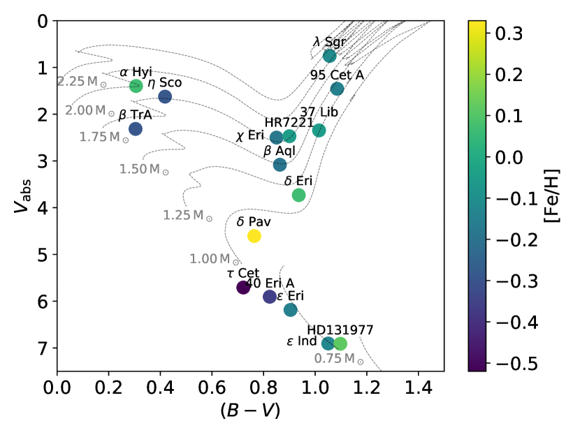
Figure 1: $(B-V)$ colour magnitude diagram for science targets with overplotted BASTI evolutionary tracks for Z$=0.058$

Table 1: Science targets

Star	HD	RAa	DECa	SpTb	$V_{\rm T}^{c}$	$H^{d}$	$T_{\rm eff}$	$\log g$	[Fe/H]	$v\sin i$	Plxa	Refs
		(hh mm ss.ss)	(dd mm ss.ss)		(mag)	(mag)	(K)	(dex)	(dex)	(km s-1)	(mas)
$\tau$ Cet	10700	01 44 02.23	-16 03 58.32	G8V	3.57	1.8	5310 $\pm$ 17	4.44 $\pm$ 0.03	-0.52 $\pm$ 0.01	1.60	277.52 $\pm$ 0.52	1,1,1,2
$\alpha$ Hyi	12311	01 58 46.77	-62 25 48.93	F0IV	2.87	1.9	7165 $\pm$ 64	3.67 $\pm$ 0.20	0.07 $\pm$ 0.10	118.00	51.55 $\pm$ 0.83	3,4,4,5
$\chi$ Eri	11937	01 55 58.59	-52 23 32.60	G8IV	3.80	1.9	5135 $\pm$ 80	3.42 $\pm$ 0.10	-0.18 $\pm$ 0.07	4.50	57.38 $\pm$ 0.33	6,6,6,7
95 Cet A	20559	03 18 22.68	-1 04 10.02	-	5.60	-	4684 $\pm$ 71	2.64 $\pm$ 0.14	-0.15 $\pm$ 0.05	1.60	15.63 $\pm$ 0.18	8,8,8,9
$\epsilon$ Eri	22049	03 32 54.82	-10 32 30.58	K2V	3.81	1.9	5049 $\pm$ 48	4.45 $\pm$ 0.09	-0.15 $\pm$ 0.03	4.08	312.22 $\pm$ 0.47	1,1,1,10
$\delta$ Eri	23249	03 43 14.80	-10 14 23.33	K0+IV	3.62	1.7	5027 $\pm$ 48	3.66 $\pm$ 0.10	0.07 $\pm$ 0.03	6.79	110.22 $\pm$ 0.42	1,1,1,10
40 Eri A	26965	04 15 13.98	-8 19 56.63	K0V	4.51	2.6	5098 $\pm$ 32	4.35 $\pm$ 0.10	-0.36 $\pm$ 0.02	2.10	198.57 $\pm$ 0.51	1,1,1,2
37 Lib	138716	15 34 11.03	-11 56 04.05	K1III-IV	4.72	2.3	4816 $\pm$ 70	3.05 $\pm$ 0.19	-0.05 $\pm$ 0.06	4.50	35.19 $\pm$ 0.25	8,8,8,9
$\beta$ TrA	141891	15 55 08.13	-64 34 03.16	F1V	2.85	2.2	7112 $\pm$ 64	4.22 $\pm$ 0.07	-0.29 $\pm$ 0.10	69.63	79.43 $\pm$ 0.58	3,11,4,10
$\lambda$ Sgr	169916	18 27 58.19	-26 34 39.01	K1IIIb	2.92	0.4	4778 $\pm$ 37	2.66 $\pm$ 0.10	-0.11 $\pm$ 0.03	3.81	38.78 $\pm$ 0.63	12,13,12,14
$\delta$ Pav	190248	20 08 46.71	-67 48 47.04	G8IV	3.62	2.0	5604 $\pm$ 38	4.26 $\pm$ 0.06	0.33 $\pm$ 0.03	0.32	164.05 $\pm$ 0.36	1,1,1,10
$\epsilon$ Ind	209100	22 03 29.14	-57 12 11.15	K5V	4.83	2.3	4649 $\pm$ 74	4.63 $\pm$ 0.01	-0.13 $\pm$ 0.06	2.00	274.80 $\pm$ 0.25	1,8,1,15
HD131977	131977	14 57 29.15	-22 34 37.56	K4V	5.88	3.1	4507 $\pm$ 58	4.76 $\pm$ 0.06	0.12 $\pm$ 0.03	7.68	170.01 $\pm$ 0.09	16,17,17,10
$\eta$ Sco	155203	17 12 09.22	-44 45 34.45	F5IV	3.36	2.3	6724 $\pm$ 106	3.65 $\pm$ 0.20	-0.29 $\pm$ 0.10	150.00	45.96 $\pm$ 0.44	18,4,4,19
$\beta$ Aql	188512	19 55 18.84	06 24 16.90	G8IV	3.81	1.9	5062 $\pm$ 57	3.54 $\pm$ 0.14	-0.19 $\pm$ 0.05	22.28	74.76 $\pm$ 0.36	8,8,8,10
HR7221	177389	19 09 53.30	-69 34 31.31	K0IV	5.41	3.1	5061 $\pm$ 26	3.49 $\pm$ 0.09	-0.05 $\pm$ 0.02	-	27.04 $\pm$ 0.09	12,12,12,-

Notes: ^aGaia Brown et al. (2018) - note that Gaia parallaxes listed here have not been corrected for the zeropoint offset, ^bSIMBAD, ^cTycho Høg et al. (2000), ^d2MASS Skrutskie et al. (2006)

References for spectroscopic $T_{\rm eff}$, $\log g$, [Fe/H], and $v\sin i$: 1. Delgado Mena et al. (2017), 2. Jenkins et al. (2011), 3. Blackwell & Lynas-Gray (1998), 4. Erspamer & North (2003), 5. Royer et al. (2007), 6. Fuhrmann et al. (2017), 7. Schröder et al. (2009), 8. Ramírez et al. (2013), 9. Massarotti et al. (2008), 10. Martínez-Arnáiz et al. (2010), 11. Allende Prieto et al. (2004), 12. Alves et al. (2015), 13. Liu et al. (2007), 14. Hekker & Meléndez (2007), 15. Torres et al. (2006), 16. Boyajian et al. (2012b), 17. Valenti & Fischer (2005), 18. Casagrande et al. (2011), 19. Mallik et al. (2003),

2.2 Calibration Strategy

The principal data product for the interferometric measurement of stellar angular diameter measurements is the fringe visibility, $V$, which can be defined as the ratio of the amplitude of interference fringes, and their average intensity as follows:

$$V=\frac{\rm fringe~{}amplitude}{\rm average~{}fringe~{}intensity}$$ (1)

where $V$ varies between 0, for completely resolved targets (e.g. resolved discs, well-separated binary components), and 1 for completely unresolved targets (i.e. a point source). $V$ is a function of both the projected baseline and the wavelength of observation, combining to give a characteristic spatial frequency at which observations are made.

When performing ground-based interferometric observations in real conditions, the combined effect of atmospheric turbulence and instrumental factors (e.g. optical aberrations) is to reduce the measured science target visibility $V_{\rm sci,measured}$ from its true value. To account for this, calibrator stars are observed to obtain a measure of the combined atmospheric and instrumental transfer function $V_{\rm system}$ in order to calibrate the $V_{\rm sci,measured}$ and determine their true value of $V_{\rm sci,corrected}$. Ideal calibrators meet four criteria: they are single unresolved point-sources to the interferometer, have no close companions or other asymmetries (e.g. oblate due to rapid rotation), and are both proximate on sky and close in magnitude to the science target. Being close on sky ensures they are similarly affected by atmospheric turbulence (and thus suffer from the same systematics), and similar in magnitude ensures the detector can be operated in the same mode (e.g. same exposure time and gain). Their status of isolated or single stars means that their observation is insensitive to projected baseline geometry.

With all of these criteria met, and calibrator observations taking place immediately before or after science target observations, the measured calibrator visibility $V_{\rm cal,measured}$ can be used to determine $V_{\rm system}$ provided a prediction of the true calibrator visibility $V_{\rm cal,predicted}$ is available in the from of a predicted limb darkened angular diameter $\theta_{\rm LD,cal}$. In practice the significance of the dependency on knowing the (typically unmeasured) diameter of a calibrator is minimised by choosing calibrators much smaller in angular size than their respective science targets (ideally $\theta_{\rm LD,cal}\leq\frac{1}{2}\theta_{\rm LD,sci}$ in practice), such that even large $\theta_{\rm LD,cal}$ uncertainties do not significantly change $V_{\rm cal,measured}$ for the mostly/entirely unresolved calibrator. This is formalised below in Equations 2 and 3:

$$V_{\rm sci,corrected}=\frac{V_{\rm tar,measured}}{V_{\rm system}}$$ (2)

with

$$V_{\rm system}=\frac{V_{\rm cal,measured}}{V_{\rm cal,predicted}}$$ (3)

This is not feasible in practice, particularly for stars as bright as those considered here, where it is difficult to find unresolved (yet bright) neighbouring stars. Given this limitation, the decision was made to observe a total of five calibrators per science target which, on average, meet the criteria. This lead to the observation of two separate CAL-SCI-CAL-SCI-CAL sequences - one for bright, but often more distant and resolved, stars, and another for those more faint, but closer and less resolved. Calibrators from bright and faint sequences have $\theta_{\rm LD,cal}$, on average, $0.59\theta_{\rm LD,sci}$, and $0.47\theta_{\rm LD,sci}$ respectively. This large number of calibrators allows for the possibility of unforeseen bad calibrators (e.g. resolved binaries) without compromising on the ability to calibrate the scientific observations.

Calibrators were selected using SearchCal (Bonneau et al., 2006; Bonneau et al., 2011), and the pavo_ptsrc IDL calibrator code (maintained within the CHARA/PAVO collaboration), with the the list of calibrators used detailed in Table 6.

Interstellar extinction was computed for stars more distant than 70 pc using intrinsic stellar colours from Pecaut & Mamajek (2013) for the main sequence and Aller et al. (1982) for spectral types III, II, Ia, Ib, with the subgiant branch interpolated as being halfway between spectral types V and III. We note that this approach is, at best, an approximation, but more complete or modern catalogues of intrinsic stellar colours are not available, and 3-dimensional dust maps (e.g. Green et al., 2015, 2018) are incomplete for the southern hemisphere. With intrinsic colours in hand, $B$, $V$, $H_{\rm P}$, $B_{\rm T}$, $V_{\rm T}$, and $R_{\rm P}$ photometry could be corrected for the effect of reddening using the extinction law of Cardelli et al. (1989) implemented in the extinction python package. This approach was not applied to WISE photometry however for the joint reasons of being less subject to extinction in the infrared, and what extinction (or even emission, e.g. Fritz et al., 2011) occurs being difficult to parameterise and not covered by the same relations that hold at optical wavelengths.

Angular diameters for calibrators were predicted using surface brightness relations from Boyajian et al. (2014), prioritising those with WISE $W3$ or $W4$ magnitudes to minimise the effect of interstellar reddening. A $(V-W3)$ relation was used for 59 stars, the majority of our calibrator sample, with Johnson $V$ band magnitudes converted from $Tycho-2$ catalogue $V_{\rm T}$ band (Høg et al., 2000) per the conversion outlined in Bessell (2000), and another three with unavailable or saturated $W3$ using a $(V-W4)$ relation.

The remaining three stars lacked WISE magnitudes altogether, and whilst a $(B-V)-$[Fe/H] relation (converting $B_{\rm T}$ to $B$, also per Bessell 2000) from Boyajian et al. (2014) was used for HD 16970A ([Fe/H]=0.0, Gray et al. 2003), HD 20010A and HD 24555 lack literature measurements of [Fe/H] which the simpler $(B-V)$ relation is highly sensitive to. To get around both this sensitivity and the saturated nature of 2MASS photometry for such bright stars, $(V-K)$ was computed from $(V_{\rm T}-R_{\rm P})$ via a third order polynomial fit to the photometry of a million synthetic stars ($4,500<T_{\rm eff}<7,500$, $2<\log g<5$, $-1<[Fe/H]<0.5$) using the methodology and software of Casagrande & VandenBerg (2014, 2018a). This fit was:

$$Y=0.2892625+0.643771X+2.5184359X^{2}-1.121815X^{3}$$ (4)

where $Y$ and $X$ are the $(V-K)$ and $(V_{\rm T}-R_{\rm P})$ colours respectively.

2.3 Interferometric Observations

VLTI (Haguenauer et al., 2010) PIONIER (Bouquin et al., 2011) observations were undertaken in service mode during ESO periods 99, 101, and 102 (2017-2019), using the four 1.8 m Auxiliary Telescopes on the two largest configurations: A0-G1-J2-J3 and A0-G1-J2-K0 (58-132 m and 49-129 m baselines respectively). The service mode observations had the constraint of clear skies and better than 1.2 arcsec seeing. Two 45 min CAL-SCI-CAL-SCI-CAL sequences were observed per target, with each target having five calibrator stars in total (with one shared between each sequence). In practice this looked something like CAL1-SCI-CAL2-SCI-CAL3 and CAL1-SCI-CAL4-SCI-CAL5, but with the calibrators in each sequence ordered by their respective sidereal time constraints (i.e. by taking into account shadowing from the four Unit Telescopes). PIONIER was operated in GRISM mode (6 spectral channels) for the entirety of the program.

PIONIER observations are summarised in Table 2. Note that $\delta$ Eri, 40 Eri A, and $\beta$ TrA were reobserved to complete both bright and faint sequences, with both $\tau$ Cet, and $\epsilon$ Ind serving as useful inter-period diagnostics of identical sequences.

We note that all targets had sequences observed over at least two nights, with the exception of 37 Lib and $\beta$ Aql which had their bright and faint sequences observed on the same night. As discussed in detail by Lachaume et al. (2019), there are correlated uncertainties for observations taken within a given night (e.g. atmospheric effects, instrumental drifts), reducing the accuracy of the resulting diameter fits. The consequence of this for these two stars is that any systematics in wavelength scale calibration are the same for both sequences.

Table 2: Observing log. Note that five unique calibrators were observed per science target, though some later needed to be excluded due to factors such as binarity.

Star	UT Date	ESO	Sequence	Baseline	Calibrator	Calibrators
		Period	Type		HD	Used
$\epsilon$ Ind	2017-07-22	99	faint	A0-G1-J2-K0	205935, 209952, 212878	3
$\alpha$ Hyi	2017-07-24	99	faint	A0-G1-J2-K0	1581, 15233, 19319	2
$\chi$ Eri	2017-07-24	99	bright	A0-G1-J2-K0	1581, 11332, 18622	2
$\beta$ TrA	2017-07-25	99	bright	A0-G1-J2-K0	128898, 136225, 165040	3
37 Lib	2017-07-25	99	bright	A0-G1-J2-K0	132052, 141795, 149757	3
37 Lib	2017-07-25	99	faint	A0-G1-J2-K0	136498, 139155, 149757	3
$\alpha$ Hyi	2017-07-26	99	bright	A0-G1-J2-J3	1581, 11332, 18622	2
$\chi$ Eri	2017-07-27	99	faint	A0-G1-J2-J3	10019, 11332, 18622	2
$\epsilon$ Ind	2017-08-17	99	bright	A0-G1-J2-K0	197051, 209952, 219571	3
$\tau$ Cet	2017-08-17	99	faint	A0-G1-J2-K0	9228, 10148, 18978	3
$\lambda$ Sgr	2017-08-26	99	faint	A0-G1-J2-J3	166464, 167720, 175191	2
$\tau$ Cet	2017-08-26	99	bright	A0-G1-J2-J3	9228, 17206, 18622	2
95 Cet A	2017-08-26	99	bright	A0-G1-J2-J3	16970A, 19994, 22484	3
$\delta$ Pav	2017-08-27	99	faint	A0-G1-J2-J3	192531, 197051, 197359	3
95 Cet A	2017-09-01	99	faint	A0-G1-J2-J3	16970A, 19866, 20699	3
$\epsilon$ Eri	2017-09-04	99	faint	A0-G1-J2-J3	16970A, 21530, 25725	2
40 Eri A	2017-09-04	99	faint	A0-G1-J2-J3	24780, 26409, 27487	3
$\epsilon$ Eri	2017-09-05	99	bright	A0-G1-J2-J3	16970A, 20010A, 24555	3
$\lambda$ Sgr	2017-09-08	99	bright	A0-G1-J2-J3	165634, 169022, 175191	2
$\delta$ Pav	2017-09-12	99	bright	A0-G1-J2-J3	169326, 197051, 191937	3
$\delta$ Eri	2017-09-24	99	faint	A0-G1-J2-J3	16970A, 23304, 26464	3
$\beta$ TrA	2018-04-18	101	faint	A0-G1-J2-J3	128898, 140018, 143853	3
$\beta$ Aql	2018-06-04	101	bright	A0-G1-J2-J3	182835, 189188, 194013	3
$\beta$ Aql	2018-06-04	101	faint	A0-G1-J2-J3	182835, 193329, 189533	3
$\epsilon$ Ind	2018-06-04	101	bright	A0-G1-J2-J3	197051, 209952, 219571	3
HD131977	2018-06-05	101	faint	A0-G1-J2-J3	129008, 133649, 133670	3
HR7221	2018-06-05	101	bright	A0-G1-J2-J3	161955, 165040, 188228	3
$\epsilon$ Ind	2018-06-06	101	faint	A0-G1-J2-J3	205935, 209952, 212878	3
$\eta$ Sco	2018-06-06	101	bright	A0-G1-J2-J3	135382, 158408, 160032	2
HD131977	2018-06-06	101	bright	A0-G1-J2-J3	129502, 133627, 133670	3
HR7221	2018-06-06	101	faint	A0-G1-J2-J3	165040, 172555, 173948	2
$\eta$ Sco	2018-06-07	101	faint	A0-G1-J2-J3	152236, 152293, 158408	1
$\tau$ Cet	2018-08-06	101	bright	A0-G1-J2-J3	4188, 9228, 17206	3
$\beta$ TrA	2018-08-07	101	bright	A0-G1-J2-J3	128898, 136225, 165040	3
$\tau$ Cet	2018-08-07	101	faint	A0-G1-J2-J3	9228, 10148, 18978	3
$\delta$ Eri	2018-11-25	102	bright	A0-G1-J2-J3	16970A, 20010A, 24555	3
$\delta$ Eri	2018-11-26	102	faint	A0-G1-J2-J3	16970A, 23304, 26464	3
40 Eri A	2018-11-26	102	bright	A0-G1-J2-J3	26409, 26464, 33111	3
40 Eri A	2018-11-26	102	faint	A0-G1-J2-J3	24780, 26409, 27487	3

2.4 Wavelength Calibration

The accuracy of model fits to visibility measurements depends not only on the uncertainties in the observed visibilities, but the spatial frequencies at which we measure them. The spatial frequencies here are also the working resolution of the interferometer, and any uncertainties in the baseline length or wavelength scale will affect the results. Uncertainties in the wavelength scale dominate this, with the effective wavelength conservatively having an accuracy of $\pm 1\%$ (Bouquin et al., 2011) or even $\pm 2\%$ (per the PIONIER manual), whereas the VLTI baseline lengths are known to cm precision resulting in an uncertainty of $\pm 0.02\%$ for the shortest baselines.

PIONIER’s spectral dispersion is known to change with time, and is calibrated once per day by the instrument operations team at Paranal. This calibration is identical to a single target observation in all respects save its use of an internal laboratory light source, with the resulting fringes used as a Fourier transform spectrometer to measure the effective wavelength of each channel. Effective wavelengths, accurate to $\sim$$1.5\%$, are then assumed ‘constant’ for all subsequent observations that night. Calibration data were downloaded from the ESO Archive where, at least for service mode observations, they are stored under the program ID 60.A-9209(A).

Another aspect of instrumental stability to be considered is whether the piezo hardware used to construct each interferometric scan of path delay is constant with respect to time. This is not a standard part of the instrument’s daily calibration routine however, and PIONIER lacks the internal laser source required to simply perform this procedure. As such, particularly given the potential for this being a limiting factor in high precision observations, several studies have sought to investigate the stability of PIONIER via a variety of means.

Kervella et al. (2017), seeking to measure the radii and limb darkening of $\alpha$ Centauri A and B, were limited by this uncertainty, and spent time investigating both its magnitude and long term stability. They used the binary system HD 123999, well constrained from two decades of monitoring (Boden et al., 2000, 2005; Tomkin & Fekel, 2006; Konacki et al., 2010; Behr et al., 2011), as a dimensional calibrator, and compared literature orbital solutions to those derived from their PIONIER observations. The result was a wavelength scaling factor determined through comparison of best-fit semi-major axis values from Boden et al. (2005), Konacki et al. (2010), and the authors’ of $\gamma=1.00481\pm 0.00412$, where $\gamma$ is a multiplicative offset in the PIONIER wavelength scale, and its uncertainty the fractional standard deviation of each measurement of the semi-major axis. This uncertainty of $0.41\%$ was then added in quadrature with all derived angular diameters instead of the 2% quoted in the PIONIER manual. These results were also found to be consistent (within $0.8\sigma$) with another binary, HD 78418, also studied by Konacki et al. (2010) yielding $\gamma=1.00169$, though with only two points this served only as a check.

Gallenne et al. (2018), as part of their investigation into red-clump stars, also spent time confirming the wavelength scale of PIONIER using a different approach: through spectral calibration in conjunction with the second generation VLTI instrument GRAVITY (Eisenhauer et al., 2011). Through interleaved observations with both instruments over two half nights of the previously characterised binary TZ For (Gallenne et al., 2016), they studied the orbital separation of the binary, taking advantage of GRAVITY’s internal laser reference source (accurate to $<0.02\%$) for calibration. Combining data they found a relative difference of $0.35\%$ in the measured separations, consistent with Kervella et al. (2017), which was taken to be the systematic uncertainty of the PIONIER wavelength calibration. The authors do not report a systematic offset equivalent to $\gamma$ from Kervella et al. (2017), only a relative uncertainty, with subsequent work involving authors of both investigations using only this relative value (Gallenne et al., 2019).

Lachaume et al. (2019), and the associated Rabus et al. (2019), undertook investigation into the statistical uncertainties and systematics when using PIONIER to measure diameters for under-resolved low-mass stars. They make use of the findings of Gallenne et al. (2018) and take the uncertainty on the central wavelength of each spectral channel, and thus the spatial frequency itself, to be $\pm$0.35%. Rather than applying this uncertainty to the x-axis spatial frequency values during modelling, they instead translate the error to a y-axis uncertainty in visibility. During modelling, the uncertainties are sampled and treated as a correlated systematic source of error for all observations taken on a single night with the same configuration, and uncorrelated otherwise.

With these recent results in mind, the wavelength calibration strategy for this work is to use the spectral dispersion information calibration available on each night, and adopt an uncertainty of 0.35% on our wavelength scale per the conclusions of Kervella et al. (2017) and Gallenne et al. (2018). Following the approach of subsequent investigations (Rabus et al., 2019; Lachaume et al., 2019; Gallenne et al., 2019), we do not consider a systematic offset in the wavelength scale. For the results described here, this relative uncertainty is added in quadrature with all bootstrapped angular diameter uncertainties.

2.5 Data Reduction

A single CAL-SCI-CAL-SCI-CAL sequence generates five interferogram and a single dark exposure per target (each consisting of 100 scans), plus a set of flux splitting calibration files known as a ‘kappa matrix’ (consisting of four files, each with a separate telescope shutter open). This produces 34 files per observational sequence, though this can be more in practice if more observations are required to replace those of poor quality. This raw data can be accessed and downloaded in bulk through the ESO archive .

pndrs Bouquin et al. (2011), the standard PIONIER data reduction pipeline, was used to go from raw data to calibrated squared visibility ($V^{2}$) measurements of our science targets. During reduction the exposures are averaged together, to produce 36 V² points for each of the two science target observation (six wavelength channels on six independent baselines), resulting in 72 V² points for the entire sequence. pndrs uses the calibrators in the bracketed sequence to determine the instrumental and atmospheric transfer function by interpolating in time.

The python package reach, written for this project, was used to interface with pndrs to perform simple tasks such as providing files of calibrator estimated diameters, and using the standard pndrs script reading functionality to exclude bad calibrators (e.g. binaries) or baselines (e.g. lost tracking) from being using for calibration. reach also exists to perform the more complex task of accurate $V^{2}$ uncertainty estimation considering correlated or non-Gaussian errors. Similar to the approach of Lachaume et al. (2014); Lachaume et al. (2019), we perform a bootstrapping algorithm on the calibrated interferograms within each given CAL-SCI-CAL-SCI-CAL sequence, in combination with Monte Carlo sampling of the predicted calibrator angular diameters, and science target stellar parameters ($T_{\rm eff}$, $\log g$, and [Fe/H]) and magnitudes, for calculation of limb darkening coefficients, bolometric fluxes (see Sections 3.1-3.5), radii, and luminosities.

Our bootstrapping implementation samples (with repeats) the five interferograms of each science or calibrator target in the sequence independently, rather than sampling from the combined 10 science and 15 calibrator interferograms respectively. In addition, predicted calibrator angular diameters are sampled at each step from a normal distribution using the uncertainties on the colour-angular diameter relations. The results as presented here were bootstrapped 5,000 times, fitting for both $\theta_{\rm UD,sci}$ and $\theta_{\rm LD,sci}$, and calculating $f_{\rm bol}$, $T_{\rm eff}$, radius ($R$), and luminosity ($L$) once per iteration. Final values for each parameter, as well as each ${V_{\rm tar,corrected}}^{2}$ point (for the plots in Figure 2), and their uncertainties were calculated through the mean and standard deviations of the resulting probability distributions. The Monte-Carlo/diameter fitting process was then completed once more in its entirety, but sampling our interferometry derived $T_{\rm eff}$ values in place of their literature equivalents from Table 1. The effect of this is for our limb darkening coefficients and bolometric fluxes to be sampled with less scatter by using values with smaller and more consistent uncertainties, in effect ‘converging’ to the final reported values in Table 4.

3 Results

3.1 Limb Darkened Angular Diameters

A linearly-limb darkened disc model is a poor fit to both real and model stellar atmospheres, but in order to properly resolve the intensity profile and take advantage of higher order limb darkening laws (e.g. Equation 5 below, from Claret 2000), one must resolve beyond the first lobe of the visibility profile:

$$\frac{I(\mu)}{I(1)}=1-\sum_{k=1}^{4}a_{k}(1-\mu^{\frac{k}{2}})$$ (5)

where $I(1)$ is the specific intensity at the centre of the stellar disc, $\mu=\cos\left(\gamma\right)$ with angle $\gamma$ between the line of sight and emergent intensity, $k$ the polynomial order, and $a_{k}$ the associated coefficient.

In the first and second lobes, the visibilities of a 4-term limb darkening law are nearly indistinguishable from linearly darkened model of slightly different diameter and appropriate coefficient. We thus model the intensity profile with a four term law, interpolating the 3D stagger grid of model atmospheres (Magic et al., 2015) initially with the $T_{\rm eff}$, $\log g$, and [Fe/H] given in Table 1, then a second and final time using the resulting estimate of the interferometric $T_{\rm eff}$. Note that stagger assumes $v\sin i=0\,$km s^-1, however the fastest rotating stars in our sample are too hot for the grid (discussed below), minimising the influence of this limitation.

For the results presented here, obtained at the highest resolution possible at the VLTI, we resolve only the first lobe for all stars bar $\lambda$ Sgr (see Section 3.2). This means that we do not resolve the intensity profile well enough to take full advantage of higher order polynomial limb darkening laws. Given this limitation, the best approach, which can be considered analogous to reducing the resolution of the model to the resolution of the data available, would be an equivalent linear coefficient to the four term model described above. The so called ‘equivalent linear coefficient’ is the coefficient that gives the same side-lobe height for both models, though with a slightly smaller value of $\theta_{\rm LD}$ of the order $0.4-0.5\%$, corrected for by the scaling factor $s_{\lambda}$. This is formalised in White et al. (in prep).

For each target we fitted a modified linearly limb darkened disc model per Hanbury Brown et al. (1974):

$$V^{2}=C{\Bigg{(}\bigg{(}\frac{1-u_{\lambda}}{2}+\frac{u_{\lambda}}{3}\bigg{)}^{-1}\bigg{[}(1-u_{\lambda})\frac{J_{1}(x)}{x}+u_{\lambda}(\pi/2)^{1/2}\frac{J_{3/2}(x)}{x^{3/2}}\bigg{]}\Bigg{)}}^{2}$$ (6)

with

$$x=\pi Bs_{\lambda}\theta_{\rm LD}\lambda^{-1}$$ (7)

where $V$ is the calibrated fringe visibility, $C$ is an intercept scaling term, $u_{\lambda}$ is the wavelength dependent linear limb darkening coefficient, $s_{\lambda}$ the wavelength dependent diameter scaling term, $J_{n}(x)$ is the $n^{th}$ order Bessel function of the first kind, $B$ is the projected baseline, and $\lambda$ is the observational wavelength. Fitting was performed using scipy’s fmin minimisation routine with a $\chi^{2}$ loss function.

The intercept term $C$, and diameter scaling parameter $s_{\lambda}$, are the sole modifications to the standard linearly darkened disc law. In the ideal case where all calibrators are optimal and the system transfer function is estimated perfectly, $C$ would not be required as the calibrated visibilities would never be greater than 1. With non-ideal calibrators however, the calibration is imperfect and this is no longer the case. Deviations from $V^{2}\leq 1$ are generally small, but in the case of our bright science targets with faint calibrators, pndrs had significant calibration issues, something discussed further in Section 3.3. Thus whilst the fitting was done simultaneously on data from all sequences, each sequence of data was fit with a separate value of $C$. We also fit for the uniform disc diameter $\theta_{\rm UD}$ using Equation 6, but set $u_{\lambda}=0$ for the case of no limb darkening.

Usage of the stagger grid also confers another advantage: the ability to compute $u_{\lambda}$ for each wavelength channel of PIONIER, rather than the grid being defined broadly for the entire $H$-band as in Claret & Bloemen (2011). Thus when fitting Equation 6, $u_{\lambda}$ is actually a vector of length 6 - one for each of the PIONIER wavelength channels ($\lambda\approx 1.533,1.581,1.629,1.677,1.7258,1.773\,\mu$m). stagger however covers a limited parameter space, with the coolest stars in our sample ($\epsilon$ Ind, HD 131977), and the hottest ($\alpha$ Hyi, $\eta$ Sco, $\beta$ Aql), falling outside the grid bounds. For these stars, the grid of Claret & Bloemen (2011) is interpolated (with microturbulent velocity of $2\,$km s^-1) for the sampled parameters and used instead, which in practice means $u_{\lambda,1-6}$ are identical, and $s_{\lambda,1-6}=1.0$. Table 9 quantifies the difference in $\theta_{\rm LD}$ obtained using each of these two approaches.

Figure 2 shows $V^{2}$ fits for each of our science targets, with point colour corresponding to the observational wavelength (where darker points correspond to redder wavelengths). Note that fitting for both $\theta_{\rm UD}$ and $\theta_{\rm LD}$ was done once per bootstrapping iteration, such that these plots use the mean and standard deviations of the final distributions for each $V^{2}$ point, $C$, $u_{\lambda}$, $s_{\lambda}$, and $\theta_{\rm LD}$. To aid readability by showing only a single diameter fit for each star, each sequence of data has been normalised by its corresponding value of $C$.

Final values for $\theta_{\rm UD}$ and $\theta_{\rm LD}$ fits, with the systematic uncertainty of PIONIER’s wavelength scale added in quadrature, are presented in Table 4, and adopted $u_{\lambda}$ and $s_{\lambda}$ in Table 10.

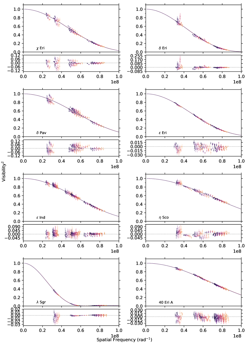
Figure 2: $V^{2}$ fits using final means and standard deviations from bootstrapped distributions. Point colour corresponds to one of the six PIONIER wavelength channels, with darker points being redder wavelengths.

Figure 3: continued

3.2 Limb Darkening of $\lambda$ Sgr

Figure 4 shows a zoomed in plot of the $\lambda$ Sgr fit, focusing on the resolved sidelobe. Comparing the model fits to the uniform disc curve, the effect of limb darkening is clear. However, with only a single star from our sample being this well resolved, it is difficult to comment on whether the observed limb darkening is consistent with models. Using PIONIER Kervella et al. (2017) found their $\alpha$ Centauri A and B results to be significantly less limb darkened than both 1D and 3D model atmosphere predictions. A similar investigation at the CHARA Array is ongoing, with results to be published as White et al. (in prep).

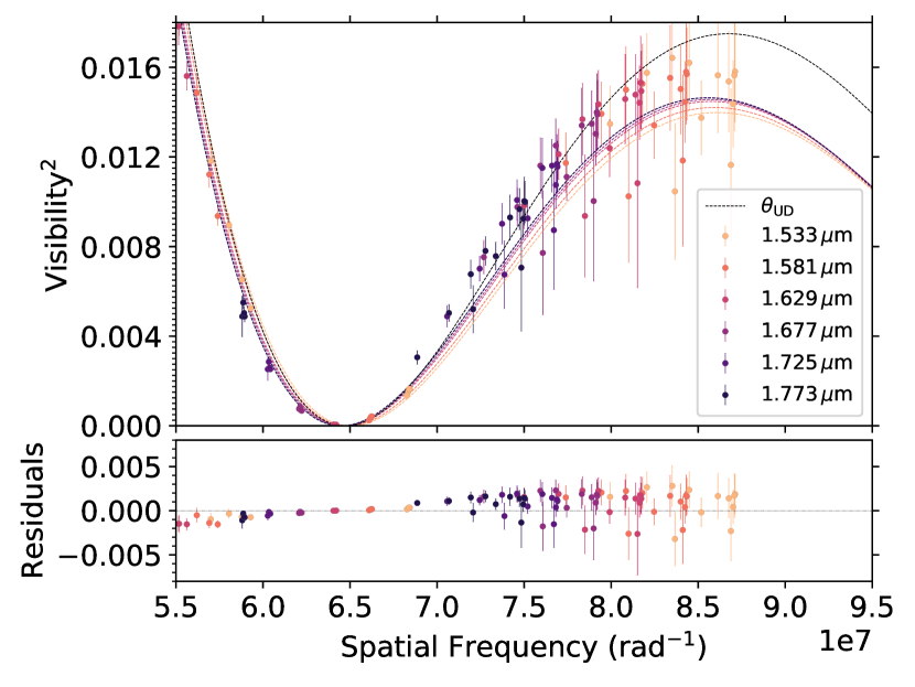
Figure 4: Zoomed in view of $\lambda$ Sgr sidelobe and limb darkening effects.

3.3 Transfer Function Calibration

In the case of perfect calibration, that is to say the influence of the system transfer function on the measured visibilities has been entirely removed, $V^{2}$ should be $0\leq V^{2}\leq 1$ and consistent with a limb darkened disc model for single stars. For many of our sequences, this was not the case, resulting in significant calibration issues where measured $V^{2}$ was systematically higher than the model, necessitating our modification of the intercept for the standard linear limb darkening law in Equation 6.

Table 3 shows the best fit intercept parameter for each observational sequence, where every star in a given sequence was observed with the same integration time. Recalling that bright sequences were those preferencing similarity in science and calibrator target magnitudes, and faint sequences were those prioritising science-calibrator on-sky separation, our mean $C$ values are as follows: $C_{\rm bright}=1.04\pm 0.03$, $C_{\rm faint}=1.05\pm 0.03$. This difference is marginal, but is not without precedent (as discussed below), and indeed non-linear behaviour at high visibility due to the difference in brightness between science and calibrator is a known, if unaddressed, issue with PIONIER.

Wittkowski et al. (2017) encountered high $V^{2}$ at short baselines, systematically above model predictions, when imaging both the carbon AGB star R Scl ($H{\sim}0.49$), and the nearby resolved K5/M0 giant $\upsilon$ Cet ($H{\sim}0.27$) for comparison and validation. Both targets were observed with the same selection of calibrators: HD 6629 ($H{\sim}2.90$), HR 400 ($H{\sim}1.85$), $\xi$ Scl ($H{\sim}2.65$), HD 8887 ($H{\sim}4.29$), HD 9961 ($H{\sim}3.91$), HD 8294 ($H{\sim}4.36$), and HR 453 ($H{\sim}3.72$), on average being nearly 3 magnitudes fainter than the science and check targets. They conclude the systematic as being most likely caused by either this difference in magnitude or airmasses between the science and calibrator targets, and took it into account by excluding the short baseline $V^{2}$ data during modelling and image synthesis.

Observations to image granulation on $\pi$ Gru ($H{\sim}-1.71$) in Paladini et al. (2018) were also subject to the same systematic. The two calibrators used, HD 209688 ($H{\sim}1.44$) and HD 215104 ($H{\sim}2.61$), were both substantially fainter than the science target by $\geq 3$ magnitudes. The authors do not go into detail about how they addressed the miscalibration other than adding a flat 5% systematic relative uncertainty to their data.

The corresponding mean difference between our science target and ‘good’ (i.e. used) calibrator magnitudes in $H$ is $\Delta H_{\rm bright}=0.95$, and $\Delta H_{\rm faint}=1.69$. If the issue indeed stems from $\Delta H$ being large, then the marginal difference we observe in $C$ is at least consistent with the bright sequences on average having a lower $\Delta H$.

Table 3: Fitted intercept parameter $C$ for each observational sequence.

Star	Period	Sequence	$C_{\rm LD}$	$C_{\rm UD}$
37 Lib	99	bright	1.007 $\pm$ 0.007	1.006 $\pm$ 0.007
37 Lib	99	faint	1.045 $\pm$ 0.006	1.045 $\pm$ 0.006
95 Cet A	99	bright	1.028 $\pm$ 0.010	1.027 $\pm$ 0.010
95 Cet A	99	faint	1.064 $\pm$ 0.006	1.063 $\pm$ 0.006
HD131977	101	bright	1.009 $\pm$ 0.007	1.009 $\pm$ 0.007
HD131977	101	faint	1.034 $\pm$ 0.009	1.034 $\pm$ 0.009
HR7221	101	bright	1.032 $\pm$ 0.008	1.031 $\pm$ 0.008
HR7221	101	faint	1.010 $\pm$ 0.007	1.009 $\pm$ 0.007
$\tau$ Cet	99	bright	1.021 $\pm$ 0.013	1.018 $\pm$ 0.013
$\tau$ Cet	101	bright	1.067 $\pm$ 0.012	1.064 $\pm$ 0.012
$\tau$ Cet	99	faint	1.108 $\pm$ 0.014	1.105 $\pm$ 0.014
$\tau$ Cet	101	faint	1.072 $\pm$ 0.011	1.070 $\pm$ 0.011
$\alpha$ Hyi	99	bright	1.044 $\pm$ 0.008	1.043 $\pm$ 0.008
$\alpha$ Hyi	99	faint	1.016 $\pm$ 0.018	1.015 $\pm$ 0.018
$\beta$ Aql	101	bright	1.017 $\pm$ 0.008	1.014 $\pm$ 0.008
$\beta$ Aql	101	faint	1.051 $\pm$ 0.010	1.048 $\pm$ 0.010
$\beta$ TrA	99	bright	1.064 $\pm$ 0.010	1.064 $\pm$ 0.010
$\beta$ TrA	101	bright	1.090 $\pm$ 0.007	1.089 $\pm$ 0.007
$\beta$ TrA	101	faint	1.041 $\pm$ 0.009	1.040 $\pm$ 0.009
$\chi$ Eri	99	bright	1.090 $\pm$ 0.022	1.087 $\pm$ 0.022
$\chi$ Eri	99	faint	1.073 $\pm$ 0.009	1.070 $\pm$ 0.009
$\delta$ Eri	102	bright	1.091 $\pm$ 0.023	1.084 $\pm$ 0.023
$\delta$ Eri	99	faint	1.055 $\pm$ 0.006	1.050 $\pm$ 0.006
$\delta$ Eri	102	faint	1.020 $\pm$ 0.005	1.015 $\pm$ 0.005
$\delta$ Pav	99	bright	1.049 $\pm$ 0.022	1.048 $\pm$ 0.022
$\delta$ Pav	99	faint	1.018 $\pm$ 0.029	1.017 $\pm$ 0.029
$\epsilon$ Eri	99	bright	1.011 $\pm$ 0.008	1.008 $\pm$ 0.008
$\epsilon$ Eri	99	faint	1.049 $\pm$ 0.008	1.046 $\pm$ 0.008
$\epsilon$ Ind	99	bright	1.004 $\pm$ 0.008	1.003 $\pm$ 0.008
$\epsilon$ Ind	101	bright	1.043 $\pm$ 0.009	1.042 $\pm$ 0.009
$\epsilon$ Ind	99	faint	1.080 $\pm$ 0.024	1.079 $\pm$ 0.024
$\epsilon$ Ind	101	faint	1.005 $\pm$ 0.008	1.003 $\pm$ 0.008
$\eta$ Sco	101	bright	1.061 $\pm$ 0.010	1.060 $\pm$ 0.010
$\eta$ Sco	101	faint	1.169 $\pm$ 0.029	1.169 $\pm$ 0.029
$\lambda$ Sgr	99	bright	1.029 $\pm$ 0.027	0.994 $\pm$ 0.027
$\lambda$ Sgr	99	faint	1.036 $\pm$ 0.022	1.003 $\pm$ 0.023
40 Eri A	102	bright	0.998 $\pm$ 0.011	0.997 $\pm$ 0.011
40 Eri A	99	faint	1.078 $\pm$ 0.006	1.077 $\pm$ 0.006
40 Eri A	102	faint	1.045 $\pm$ 0.005	1.043 $\pm$ 0.005

3.4 Bolometric Fluxes

Determination of $T_{\rm eff}$ requires measurement of $f_{\rm bol}$, the bolometric flux received at Earth, which can be done through one of several techniques, each with precedent in optical interferometry literature. All are only accurate to the few percent level, primarily due to uncertainties on the adopted zero points used to convert fluxes, either real or synthetic, to magnitudes and vice versa.

The least model dependent approach is to use a combination of spectrophotometry and broadband photometry from the science target itself, in combination with synthetic equivalents for missing or contaminated regions, to construct the flux calibrated spectral energy distribution of the star from which $f_{\rm bol}$ can be determined. White et al. (2018) implemented this procedure, using the methodology outlined in Mann et al. (2015).

A related technique is to employ a library of flux calibrated template spectra covering a range of spectral types, e.g. the Pickles Atlas (115-2500 nm, Pickles 1998), in lieu of spectrophotometry from the targets themselves. Fits are then performed to target broadband photometry using library spectra of adjacent spectral types. This was the approach taken by e.g. van Belle et al. (2007, 2008); Boyajian et al. (2012a, b, 2013); White et al. (2013), which lacks the limitations associated with synthetic spectra (e.g. due to modelling assumptions such as one-dimensional and hydrostatic models, or models satisfying local thermodynamic equilibrium). However, it is limited in its use of a relatively coarse, non-interpolated grid of only 131 spectra of mostly Solar metallicity, with potential errors from reddened spectra and correlated errors associated with the photometric calibration.

In lieu of a template library, the previous approach can be conducted using a grid of purely synthetic spectra. By linearly interpolating the spectral grid in $T_{\rm eff}$, $\log g$, and [Fe/H] and fitting to available broadband photometry, $f_{\rm bol}$ can be determined as the total flux from the best-fit spectrum. This was the method employed by Rabus et al. (2019), who used PHOENIX model atmospheres (Husser et al., 2013), assuming [Fe/H] $=0$ for all targets (likely to avoid degeneracies between $T_{\rm eff}$ and [Fe/H] for cool star spectra), as well as Huber et al. (2012) using the MARCS grid of model atmospheres (Gustafsson et al., 2008). This technique has the advantage of being unaffected by instrumental or atmospheric effects, and allowing for a much finer grid, but makes the results more susceptible to potential inaccuracies within the models themselves. We note however that synthetic photometry from the MARCS grid has previously been shown to be valid using the colours from both globular and open clusters, across the HR diagram and over a wide range of metallicities ($-2.4\lesssim{\rm[Fe/H]}\lesssim+0.3$, Brasseur et al. 2010; VandenBerg et al. 2010).

The final approach to be discussed here, and the one employed for this work, computes $f_{\rm bol}$ using broadband photometry and the appropriate bolometric correction derived from model atmospheres using literature values of $T_{\rm eff}$, $\log g$, and [Fe/H]. This method saw use in Karovicova et al. (2018), and in White et al. (2018) who found it to have excellent consistency with results derived from pure spectrophotometry for all but one of their stars. Casagrande & VandenBerg (2018a) evaluated the validity of using bolometric corrections in this manner by comparing results to the $\sim$1% precision CALSPEC library (Bohlin, 2007) of Hubble Space Telescope spectrophotometry. This demonstrated that bolometric fluxes could be recovered from computed bolometric corrections to the 2% level, a value typically halved when combining the results from more photometric bands (as we do here, corresponding to roughly $\pm 12.5\,$K uncertainty on $T_{\rm eff}$ for a 5,000 K star with a 1% error on flux).

Given that all have been demonstrated successfully in the literature, we opt for the bolometric correction technique because of limited available well calibrated photometry for our bright targets. Bolometric fluxes were computed for all stars by way of the bolometric-corrections software (Casagrande & VandenBerg, 2014, 2018a; Casagrande et al., 2018). For a given set of $T_{\rm eff}$, $\log g$, and [Fe/H] the software produces synthetic bolometric corrections in different filters by interpolating the MARCS grid of synthetic spectra (Gustafsson et al., 2008). $f_{\rm bol}$ is obtained using Equation 8 (Casagrande & VandenBerg, 2018a):

$$f_{\rm bol}=\frac{\pi L_{\odot}}{1.296\times 10^{9}{\rm au}}10^{-0.4({\rm BC_{\zeta}}-M_{\rm bol,\odot}+m_{\zeta}-10)}$$ (8)

where $f_{\rm bol}$ is the stellar bolometric flux received at Earth in erg s${}^{-1}\,$cm^-2, $L_{\odot}$ is the Solar bolometric luminosity in erg s^-1 (IAU 2015 Resolution B3, $3.828\times 8^{33}\,$erg s${}^{-1}\,$cm^-2), au is the astronomical unit (IAU 2012 Resolution B2, $1.495978707\times 10^{13}\,$cm), BC_ζ and m_ζ are the bolometric correction and apparent magnitudes respectively in filter band $\zeta$, and $M_{\rm bol}=4.75$ is the adopted Solar bolometric magnitude.

Calculation of $f_{\rm bol,\zeta}$ is done at each iteration of the aforementioned bootstrapping and Monte Carlo algorithm for each of $H_{\rm P}$, $B_{\rm T}$, and $V_{\rm T}$ filter bands using the sampled stellar parameters and magnitudes, overwhelmingly consistent to within $1\sigma$ uncertainties. An instantaneous value of $f_{\rm bol,final}$ is calculated by averaging the fluxes obtained from each filter, with final values obtained as the mean and standard deviation of the respective distributions. Note that, with the goal of consistency in mind, Gaia $G$, $B_{\rm P}$, and $R_{\rm P}$ were avoided due to saturation for a portion of our sample (and a magnitude-dependent offset for bright targets as noted in Casagrande & VandenBerg 2018b).

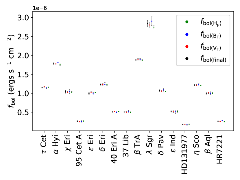
Figure 8: Comparison of $f_{\rm bol}$ calculated from Hipparcos-Tycho $H_{\rm P}$, $B_{\rm T}$, $V_{\rm T}$, as compared to the final average value adopted.

The final calculated bolometric fluxes for each band are reported in Table 8 and visualised in Figure 8, with the adopted average values in Table 4.

3.5 Fundamental Stellar Properties

The strength of measuring stellar angular diameters through interferometry is the ability to measure $T_{\rm eff}$ independent of distance in an almost entirely model independent way (the exceptions being the adopted limb darkening law, and ${\sim}1$% precision bolometric fluxes). With measures of stellar angular diameter and flux, $T_{\rm eff}$ can be calculated as follows:

$$T_{\rm eff}={\bigg{(}\frac{4f_{\rm bol}}{\sigma{\theta_{\rm LD}}^{2}}\bigg{)}}^{1/4}$$ (9)

where $T_{\rm eff}$ is the stellar effective temperature in K, $f_{\rm bol}$ is the bolometric stellar flux in ergs s${}^{-1}\,$cm^-2, and $\sigma$ is the Stefan-Boltzmann constant, taken to be $\sigma=5.6704\times 10^{-5}\,$ergs s${}^{-1}\,$cm${}^{-2}\,$K$\,{}^{-4}$.

The same measure of flux can be combined with the distance to the star to calculate the bolometric luminosity:

$$L=4\pi f_{\rm bol}D^{2}$$ (10)

where $D$ is again the distance to the star. Dividing this value by $L_{\odot}$ gives the luminosity in Solar units.

Finally, the measured angular diameter and distance can be combined to determine the physical radius of a star:

$$R=\frac{1}{2}\theta_{\rm LD}D$$ (11)

and its uncertainty:

$$\sigma_{R}=R\sqrt{{\bigg{(}\frac{\sigma_{\theta}}{\theta_{\rm LD}}\bigg{)}}^{2}+{\bigg{(}\frac{\sigma_{D}}{D}\bigg{)}}^{2}}$$ (12)

where $R$ is the physical radius of the star, $\theta_{\rm LD}$ is the limb darkened angular diameter, $D$ is the distance to the star, and $\sigma_{\theta}$ and $\sigma_{D}$ are their respective uncertainties. These can be put into Solar units using pc$=3.0857\times 10^{13}\,$km, and R${}_{\odot}=6.957\times 10^{5}\,$km.

These parameters, alongside the final angular diameters, are reported in Table 4.

Table 4: Final fundamental stellar parameters

Star	$\theta_{\rm UD}$	$\theta_{\rm LD}$	$R$	$f_{\rm bol}$	$T_{\rm eff}$	$L$
	(mas)	(mas)	($R_{\odot}$)	(10${}^{-8}\,$ergs s-1 cm -2)	(K)	($L_{\odot}$)
$\tau$ Cet	2.005 $\pm$ 0.011	2.054 $\pm$ 0.011	0.796 $\pm$ 0.004	115.0 $\pm$ 1.2	5347 $\pm$ 18	0.47 $\pm$ 0.01
$\alpha$ Hyi	1.436 $\pm$ 0.016	1.460 $\pm$ 0.016	3.040 $\pm$ 0.058	179.0 $\pm$ 3.0	7087 $\pm$ 47	21.00 $\pm$ 0.75
$\chi$ Eri	2.079 $\pm$ 0.011	2.134 $\pm$ 0.011	3.993 $\pm$ 0.027	104.0 $\pm$ 4.0	5115 $\pm$ 49	9.84 $\pm$ 0.39
95 Cet A	1.244 $\pm$ 0.012	1.280 $\pm$ 0.012	8.763 $\pm$ 0.128	26.2 $\pm$ 1.7	4678 $\pm$ 75	33.18 $\pm$ 2.27
$\epsilon$ Eri	2.087 $\pm$ 0.011	2.144 $\pm$ 0.011	0.738 $\pm$ 0.003	99.8 $\pm$ 2.5	5052 $\pm$ 33	0.32 $\pm$ 0.01
$\delta$ Eri	2.343 $\pm$ 0.009	2.411 $\pm$ 0.009	2.350 $\pm$ 0.010	123.2 $\pm$ 3.4	5022 $\pm$ 34	3.17 $\pm$ 0.09
40 Eri A	1.449 $\pm$ 0.012	1.486 $\pm$ 0.012	0.804 $\pm$ 0.006	50.8 $\pm$ 0.9	5126 $\pm$ 30	0.40 $\pm$ 0.01
37 Lib	1.639 $\pm$ 0.009	1.684 $\pm$ 0.010	5.133 $\pm$ 0.043	50.6 $\pm$ 2.6	4809 $\pm$ 62	12.71 $\pm$ 0.69
$\beta$ TrA	1.438 $\pm$ 0.013	1.462 $\pm$ 0.013	1.976 $\pm$ 0.021	188.2 $\pm$ 2.1	7171 $\pm$ 35	9.30 $\pm$ 0.17
$\lambda$ Sgr	3.910 $\pm$ 0.014	4.060 $\pm$ 0.015	11.234 $\pm$ 0.181	283.9 $\pm$ 8.7	4768 $\pm$ 36	58.79 $\pm$ 2.61
$\delta$ Pav	1.785 $\pm$ 0.025	1.828 $\pm$ 0.025	1.197 $\pm$ 0.016	107.2 $\pm$ 2.5	5571 $\pm$ 48	1.24 $\pm$ 0.03
$\epsilon$ Ind	1.758 $\pm$ 0.012	1.817 $\pm$ 0.013	0.711 $\pm$ 0.005	51.5 $\pm$ 3.7	4649 $\pm$ 84	0.21 $\pm$ 0.02
HD131977	1.098 $\pm$ 0.014	1.130 $\pm$ 0.014	0.715 $\pm$ 0.009	17.6 $\pm$ 1.1	4505 $\pm$ 76	0.19 $\pm$ 0.01
$\eta$ Sco	1.392 $\pm$ 0.017	1.416 $\pm$ 0.017	3.307 $\pm$ 0.050	121.6 $\pm$ 2.0	6533 $\pm$ 46	17.94 $\pm$ 0.45
$\beta$ Aql	2.079 $\pm$ 0.011	2.133 $\pm$ 0.012	3.064 $\pm$ 0.020	100.3 $\pm$ 2.9	5071 $\pm$ 37	5.60 $\pm$ 0.17
HR7221	1.088 $\pm$ 0.014	1.117 $\pm$ 0.015	4.428 $\pm$ 0.058	26.5 $\pm$ 0.7	5023 $\pm$ 47	11.24 $\pm$ 0.33

4 Discussion

4.1 Comparison with Previous Interferometric Measurements

Six of our sample, HD 131977, 40 Eri A, $\epsilon$ Ind, $\tau$ Ceti, $\beta$ Aql, and $\epsilon$ Eri, have literature angular diameter measurements (Table 5), which we find to be consistent with our own to within ${\sim}1\sigma$ uncertainties for all but one star (Figure 5). Our value for $\epsilon$ Ind however is substantially discrepant to the VINCI diameter by ${\sim}4\sigma$. Comparing our $V^{2}$ fits to the literature results in Demory et al. (2009) reveal that we place tighter constraints on the angular diameter by better resolving the star down to $V^{2}$ of ${\sim}0.2$ versus ${\sim}0.5$ for previous results. We expect the discrepancy is largely caused by this, plus the fact that these observations were taken at lower sensitivity using two 35 cm test siderostats during the early years of the VLTI rather than the four $1.8\,$m ATs we have access to now.

None of these prior measurements were made with PIONIER, meaning that our results offer high precision agreement between not only different VLTI beam combiners (AMBER and VINCI), but also as different facilities altogether (NPOI and CHARA/FLUOR). Given the relatively sparse overlaps however, we are not able to say anything substantial about potential systematics. We await the upcoming White et al. (in prep) which will be able to compare PIONIER to CHARA/PAVO for $\tau$ Cet, $\epsilon$ Eri, $\delta$ Eri, 37 Lib, and $\beta$ Aql. This study will also possibly enable the ability to investigate the effect of limb darkening at different wavelengths since PAVO is an $R$-band instrument, thus significantly improving the sensitivity to systematic errors. Furthermore, PAVO data for additional dwarf and giant stars, including $\beta$ Aql, but also many stars not observed here, is to be published soon in Karovicova et al. (in prep.) and a following series of papers.

Table 5: Comparison of angular diameters reported here with stars measured previously in the literature.

Star	$\theta_{\rm LD}$	Facility	Instrument	Ref
	(mas)
$\tau$ Cet	1.971 $\pm$ 0.05	VLTI	VINCI	1
	2.078 $\pm$ 0.031	VLTI	VINCI	2
	2.015 $\pm$ 0.011	CHARA	FLUOR	3
$\epsilon$ Eri	2.148 $\pm$ 0.029	VLTI	VINCI	2
	2.126 $\pm$ 0.014	CHARA	FLUOR	3
	2.153 $\pm$ 0.028	NPOI	NPOI	4
40 Eri A	1.437 $\pm$ 0.039	VLTI	AMBER	5
$\epsilon$ Ind	1.881 $\pm$ 0.017	VLTI	VINCI	5
HD131977	1.177 $\pm$ 0.029	VLTI	VINCI	5
$\beta$ Aql	2.18 $\pm$ 0.09	NPOI	NPOI	6

References. 1. Pijpers et al. (2003); 2. Di Folco et al. (2004); 3. di Folco et al. (2007); 4. Baines & Armstrong (2012); 5. Demory et al. (2009); 6. Nordgren et al. (1999)

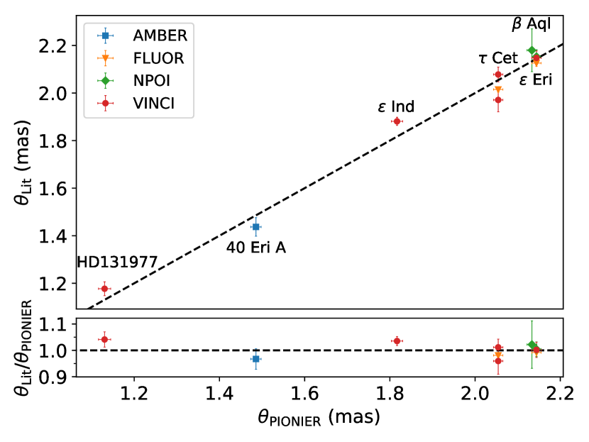
Figure 5: Comparison of PIONIER diameters as reported here, to stars with literature measurements from other interferometers or beam-combiners

4.2 Comparison with Colour-$\theta_{\rm LD}$ Relations

Figure 6 shows a comparison between our fitted diameters, and the $(V-W3)$, $(V-W4)$, and the [Fe/H] dependent $(B-V)$ colour-$\theta_{LD}$ relations from Boyajian et al. (2014) used to predict calibrator angular diameters. All three sets of relations are consistent within errors with our results (despite several of our sample being marginally too red for the [Fe/H] dependent $(B-V)$ relation), which bodes well for the accuracy of the relations. However, there appears a clear systematic offset for the $(V-W3)$ relation, plus a less severe offset for the $(V-W4)$ relation. There does not appear to be a trend in either [Fe/H] with any of these relations.

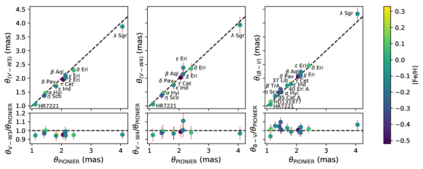
Figure 6: Comparison of $\theta_{\rm LD}$ as reported here as compared to predicted diameters from Boyajian et al. (2014). Left: $(V-W3)$ relation, Centre: $(V-W4)$ relation, Right: [Fe/H] dependent $(B-V)$ relation. Note that not all stars have WISE photometry, whereas all stars have available Tycho-2 magnitudes.

4.3 $T_{\rm eff}$ From Empirical Relations

Unfortunately comparison of the $T_{\rm eff}$ values derived here to those from IR Flux method (Casagrande et al., 2010) is not possible due to saturated 2MASS photometry - the critical source of infrared photometry. Another source of comparison is to use the empirical relations provided by the same study, which give an empirical mapping between select colour indices and $T_{\rm eff}$. Figure 7 presents $T_{\rm eff}$ as a function of $(B_{\rm T}-V_{\rm T})$, uncertainties $\pm 79\,$K, and demonstrates $1\sigma$ agreement for all stars, with the exceptions of HD 131977 and $\beta$ TrA. Inspecting the photometry for both stars, values of $f_{\rm bol}$ derived from different filter bands are consistent, and rotation does not appear to be a significant factor when considering literature $v\sin i$ presented Table 1. We note however that our interferometric temperatures are consistent with the literature spectroscopic values also listed in Table 1 for these two stars.

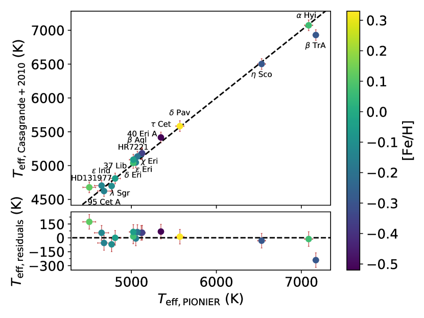
Figure 7: Comparison of $T_{\rm eff}$ as reported here and those calculated from $(B_{\rm T}-V_{\rm T})$ using the empirical relations of Casagrande et al. (2010)

5 Conclusions

We have used long-baseline optical interferometry to measure the angular diameters for a sample of 16 southern stars (6 dwarf, 5 sub-giant, and 5 giants) with exquisite precision using the PIONIER instrument on the VLTI. The limb darkened diameters reported have a mean uncertainty of $\sim$0.82$\%$, and were obtained using a robust calibration strategy, and a data analysis pipeline implementing both bootstrapping and Monte-Carlo sampling to take into account correlated uncertainties in the interferometric data. In addition to this, we also report derived $T_{\rm eff}$, physical radii, bolometric fluxes, and luminosities for all stars, with mean uncertainties of $\sim$0.9$\%$, $\sim$1.0$\%$, $\sim$3.3$\%$, and $\sim$3.7$\%$ respectively.

Ten of these stars did not have measured angular diameters prior to the results presented here, and the majority of the remaining six have values in agreement with previous literature measurements, with the sole outlier being observed at higher resolution and with greater sensitivity here. These are some of the closest and most well studied stars, and this work hopes to elevate them further to the level of spectral type standards, where they can provide constraints to theoretical models and empirical relations.

Appendix A Calibrators

Table 6: Calibrator stars

HD	SpT		$V_{\rm T}^{c}$	$H^{d}$	$E(B-V)$	$\theta_{\rm pred}$	$\theta_{\rm LD}$ Rel	Used	Plx	Target/s
	(Actual)a	(Adopted)b	(mag)	(mag)	(mag)	(mas)			(mas)
9228	K2III	K2III	6.08	3.13	0.186	1.336 $\pm$ 0.07	VW3	Y	5.99 $\pm$ 0.06e	$\tau$ Cet
10148	F0V	F0V	5.61	4.83	0.029	0.461 $\pm$ 0.02	VW3	Y	13.89 $\pm$ 0.11e	$\tau$ Cet
18978	A3IV-V	A3IV	4.09	3.54	0.000	0.719 $\pm$ 0.04	VW3	Y	38.58 $\pm$ 0.39e	$\tau$ Cet
17206	F7V	F7V	4.52	3.24	0.000	0.904 $\pm$ 0.05	VW3	Y	70.74 $\pm$ 0.45e	$\tau$ Cet
18622	-	A3IV	-	-	-	-	-	Nf	-	$\alpha$ Hyi, $\chi$ Eri, $\tau$ Cet
1581	F9.5V	F9V	4.29	2.74	0.000	1.151 $\pm$ 0.06	VW3	Y	117.17 $\pm$ 0.33e	$\alpha$ Hyi, $\chi$ Eri
15233	F2II/III	F2II	5.40	4.51	0.000	0.543 $\pm$ 0.03	VW3	Y	21.01 $\pm$ 0.10e	$\alpha$ Hyi
19319	F0III/IV	F0III	5.16	4.28	0.000	0.580 $\pm$ 0.03	VW3	Nf	23.36 $\pm$ 0.12e	$\alpha$ Hyi
11332	K0III	K0III	6.25	3.71	0.004	0.795 $\pm$ 0.04	VW3	Y	6.88 $\pm$ 0.03e	$\alpha$ Hyi, $\chi$ Eri
10019	G8III	G8III	6.95	4.76	0.013	0.573 $\pm$ 0.03	VW3	Y	5.61 $\pm$ 0.03e	$\chi$ Eri
16970A	A2Vn	A2V	3.55	-	0.000	0.754 $\pm$ 0.03	BV-feh	Y	43.60 $\pm$ 0.82e	$\delta$ Eri, $\epsilon$ Eri, 95 Cet A
19866	K0III	K0III	7.21	4.73	0.178	0.583 $\pm$ 0.03	VW3	Y	5.88 $\pm$ 0.04e	95 Cet A
20699	K0III	K0III	6.83	4.75	-0.048	0.580 $\pm$ 0.03	VW3	Y	6.24 $\pm$ 0.04e	95 Cet A
19994	F8.5V	F8V	5.13	3.77	0.000	0.785 $\pm$ 0.04	VW3	Y	44.37 $\pm$ 0.20e	95 Cet A
22484	F9IV-V	F9IV	4.35	2.92	0.000	1.127 $\pm$ 0.06	VW3	Y	71.62 $\pm$ 0.54c	40 Eri A, 95 Cet A
21530	K2II/III	K2II	5.85	3.33	-0.177	1.101 $\pm$ 0.06	VW3	Y	10.59 $\pm$ 0.09e	$\epsilon$ Eri
25725	M7+II	M7II	8.74	-0.32	-	-	VW4	Nh	2.28 $\pm$ 0.68c	$\epsilon$ Eri
20010A	F6V	F6V	3.98	2.32	0.000	1.247 $\pm$ 0.06	VK	Y	71.68 $\pm$ 0.31e	$\delta$ Eri, $\epsilon$ Eri
24555	G6.5III	G6III	4.80	2.47	-0.007	1.414 $\pm$ 0.07	VK	Y	10.11 $\pm$ 0.24e	$\delta$ Eri, $\epsilon$ Eri
23304	K0III	K0III	7.33	4.88	0.102	0.546 $\pm$ 0.03	VW3	Y	5.25 $\pm$ 0.07e	$\delta$ Eri
26464	K1III	K1III	5.81	3.55	-0.011	1.039 $\pm$ 0.05	VW3	Y	10.01 $\pm$ 0.09e	$\delta$ Eri, 40 Eri A
24780	K4/5III	K4III	8.49	4.84	0.129	0.664 $\pm$ 0.03	VW3	Y	1.66 $\pm$ 0.05e	40 Eri A
26409	G8III	G8III	5.55	3.59	0.002	1.011 $\pm$ 0.05	VW3	Y	9.10 $\pm$ 0.11e	40 Eri A
27487	G8III	G8III	6.83	4.75	-0.011	0.560 $\pm$ 0.03	VW3	Y	4.96 $\pm$ 0.04e	40 Eri A
33111	A3IV	A3IV	2.78	2.44	0.000	1.241 $\pm$ 0.06	VW3	Y	36.50 $\pm$ 0.42c	40 Eri A
136498	K2III	K2III	7.89	4.67	0.222	0.629 $\pm$ 0.03	VW3	Y	2.27 $\pm$ 0.05e	37 Lib
139155	K2/3IV	K2IV	8.64	5.00	0.472	0.548 $\pm$ 0.03	VW3	Y	1.69 $\pm$ 0.06e	37 Lib
149757	O9.2IVnn	O9IV	2.55	2.67	0.335	0.940 $\pm$ 0.05	VW3	Y	5.83 $\pm$ 1.02e	37 Lib
132052	F2V	F2V	4.50	3.82	0.000	0.753 $\pm$ 0.04	VW3	Y	36.31 $\pm$ 0.26e	37 Lib
141795	kA2hA5mA7V	A5V	3.71	3.44	0.000	0.789 $\pm$ 0.04	VW3	Y	48.08 $\pm$ 0.57e	37 Lib
128898	A7VpSrCrEu	A7V	3.19	2.47	0.000	1.157 $\pm$ 0.06	VW3	Y	62.94 $\pm$ 0.43e	$\beta$ TrA
140018	K1/2III	K1III	7.01	3.97	0.290	0.847 $\pm$ 0.04	VW3	Y	1.96 $\pm$ 0.03e	$\beta$ TrA
143853	K1III	K1III	7.24	3.92	0.268	0.706 $\pm$ 0.04	VW3	Y	2.05 $\pm$ 0.04e	$\beta$ TrA
136225	K3III	K3III	7.30	3.66	0.305	0.969 $\pm$ 0.05	VW3	Y	1.22 $\pm$ 0.04e	$\beta$ TrA
165040	kA4hF0mF2III	F0III	4.36	3.80	0.000	0.681 $\pm$ 0.03	VW3	Y	24.78 $\pm$ 0.31e	$\beta$ TrA, HR7221
166464	K0III	K0III	5.08	2.71	0.059	1.433 $\pm$ 0.07	VW3	Y	12.63 $\pm$ 0.24e	$\lambda$ Sgr
167720	K2III	K2III	5.97	2.43	0.392	1.790 $\pm$ 0.09	VW3	Y	3.02 $\pm$ 0.17e	$\lambda$ Sgr
175191	B2V	B2V	-	-	-	-	-	Nf	-	$\lambda$ Sgr
165634	G7:IIIbCN-1CH-3.5HK+1	G7III	4.66	2.19	0.010	1.620 $\pm$ 0.08	VW3	Y	9.83 $\pm$ 0.34e	$\lambda$ Sgr
169022	B9.5III	B9III	1.81	1.77	0.000	1.569 $\pm$ 0.11	VW4	Y	22.76 $\pm$ 0.24c	$\lambda$ Sgr
192531	K0III	K0III	6.40	3.85	0.055	0.781 $\pm$ 0.04	VW3	Y	7.73 $\pm$ 0.03e	$\delta$ Pav
197051	A7III	A7III	3.43	2.79	0.000	0.982 $\pm$ 0.05	VW3	Y	25.64 $\pm$ 0.33e	$\delta$ Pav, $\epsilon$ Ind
197359	K0/1III	K0III	6.82	4.47	0.074	0.674 $\pm$ 0.03	VW3	Y	6.26 $\pm$ 0.03e	$\delta$ Pav
169326	K2III	K2III	6.09	3.50	0.028	1.089 $\pm$ 0.06	VW3	Y	6.66 $\pm$ 0.08e	$\delta$ Pav
191937	K3III	K3III	6.72	3.57	0.157	1.084 $\pm$ 0.06	VW3	Y	3.99 $\pm$ 0.03e	$\delta$ Pav

Table 7: continued

Calibrator stars HD SpT $V_{\rm T}^{c}$ $H^{d}$ $E(B-V)$ $\theta_{\rm pred}$ $\theta_{\rm LD}$ Rel Used Plx Target/s (Actual)^a (Adopted)^b (mag) (mag) (mag) (mas) (mas) 205935 K0II/III K0II 6.45 3.95 -0.016 0.829 $\pm$ 0.04 VW3 Y 4.96 $\pm$ 0.03^e $\epsilon$ Ind 209952 B6V B6V 1.76 2.03 0.000 1.112 $\pm$ 0.08 VW4 Y 32.29 $\pm$ 0.21^c $\epsilon$ Ind 212878 G8III G8III 6.98 4.81 0.035 0.553 $\pm$ 0.03 VW3 Y 5.11 $\pm$ 0.04^e $\epsilon$ Ind 219571 F4V F4V 4.03 3.08 0.000 1.077 $\pm$ 0.05 VW3 Y 42.32 $\pm$ 0.25^e $\epsilon$ Ind 4188 K0III K0III 4.88 2.67 0.000 1.476 $\pm$ 0.08 VW3 Y 14.41 $\pm$ 0.37^e $\tau$ Cet 129008 G8III/IV G8III 7.25 4.88 0.029 0.546 $\pm$ 0.03 VW3 Y 5.88 $\pm$ 0.05^e HD131977 133649 K0III K0III 7.81 4.96 0.188 0.528 $\pm$ 0.03 VW3 Y 2.81 $\pm$ 0.05^e HD131977 133670 K0III K0III 6.25 3.83 0.000 0.851 $\pm$ 0.04 VW3 Y 15.41 $\pm$ 0.06^e HD131977 129502 F2V F2V 3.91 3.07 0.000 1.087 $\pm$ 0.06 VW3 Y 54.79 $\pm$ 0.51^e HD131977 133627 K0III K0III 6.86 4.33 0.041 0.709 $\pm$ 0.04 VW3 Y 6.58 $\pm$ 0.05^e HD131977 152236 B1Ia-0ek B1Ia 4.82 3.34 0.615 - - N^g 0.71 $\pm$ 0.24^e $\eta$ Sco 152293 F3II F3II 5.91 4.25 0.294 0.604 $\pm$ 0.03 VW3 Y 0.31 $\pm$ 0.16^e $\eta$ Sco 158408 B2IV B2IV 2.62 3.11 0.051 - - N^f 5.66 $\pm$ 0.18^c $\eta$ Sco 135382 A1V A1V 2.85 2.53 0.000 1.090 $\pm$ 0.06 VW3 Y 16.50 $\pm$ 0.73^e $\eta$ Sco 160032 F4V F4V 4.80 3.70 0.000 0.743 $\pm$ 0.04 VW3 Y 47.10 $\pm$ 0.29^e $\eta$ Sco 182835 F2Ib F2Ib 4.73 2.87 0.339 1.063 $\pm$ 0.05 VW3 Y 1.29 $\pm$ 0.22^e $\beta$ Aql 193329 K0III K0III 6.16 3.83 0.091 0.910 $\pm$ 0.05 VW3 Y 7.90 $\pm$ 0.07^e $\beta$ Aql 189533 G8II G8II 6.84 3.74 0.295 0.864 $\pm$ 0.04 VW3 Y 2.42 $\pm$ 0.04^e $\beta$ Aql 189188 K2III K2III 6.89 3.73 0.071 0.857 $\pm$ 0.04 VW3 Y 4.49 $\pm$ 0.04^e $\beta$ Aql 194013 G8III-IV G8III 5.41 3.31 0.038 1.143 $\pm$ 0.06 VW3 Y 12.59 $\pm$ 0.14^e $\beta$ Aql 172555 A7V A7V 4.79 4.25 0.000 0.792 $\pm$ 0.04 VW3 N^g 35.29 $\pm$ 0.23^e HR7221 173948 B2Ve B2V 4.18 4.32 0.051 0.419 $\pm$ 0.02 VW3 Y 4.80 $\pm$ 0.45^e HR7221 161955 K0/1III K0III 6.58 4.10 0.100 0.746 $\pm$ 0.04 VW3 Y 6.85 $\pm$ 0.04^e HR7221 188228 A0Va A0V 3.94 3.76 0.000 0.571 $\pm$ 0.03 VW3 Y 31.87 $\pm$ 0.33^e HR7221 Notes: ^aSIMBAD, ^bAdopted for intrinsic colour grid interpolation,^cTycho Høg et al. (2000), ^d2MASS Skrutskie et al. (2006), ^eGaia Brown et al. (2018), ^fBinarity, ^gIR excess, ^hInconsistent photometry

Appendix B Bolometric Fluxes

Table 8: Calculated bolometric fluxes

Star	HD	$f_{\rm bol}$ (MARCS)	$\sigma_{f_{\rm bol}}(\zeta)$
		(10${}^{-8}\,$ergs s-1 cm -2)	(%)
$\tau$ Cet	10700	$<>$: 114.976	1.08
		Hp: 116.099	0.40
		BT: 114.227	1.64
		VT: 116.981	0.94
$\alpha$ Hyi	12311	$<>$: 178.994	1.66
		Hp: 175.530	1.12
		BT: 181.304	2.23
		VT: 177.571	1.43
$\chi$ Eri	11937	$<>$: 103.957	3.85
		Hp: 102.641	2.02
		BT: 104.834	5.15
		VT: 102.741	2.33
95 Cet A	20559	$<>$: 26.195	6.37
		Hp: 26.783	3.91
		BT: 25.803	8.16
		VT: 25.088	4.65
$\epsilon$ Eri	22049	$<>$: 99.817	2.52
		Hp: 101.793	1.36
		BT: 98.500	3.40
		VT: 102.539	1.76
$\delta$ Eri	23249	$<>$: 123.239	2.75
		Hp: 122.583	1.45
		BT: 123.676	3.66
		VT: 123.326	1.82
40 Eri A	26965	$<>$: 50.797	1.84
		Hp: 51.708	0.92
		BT: 50.189	2.56
		VT: 52.095	1.31
37 Lib	138716	$<>$: 50.601	5.23
		Hp: 49.763	3.00
		BT: 51.159	6.76
		VT: 50.133	3.54
$\beta$ TrA	141891	$<>$: 188.174	1.14
		Hp: 187.285	0.82
		BT: 188.766	1.60
		VT: 189.549	1.20
$\lambda$ Sgr	169916	$<>$: 283.889	3.08
		Hp: 274.369	1.77
		BT: 290.236	3.99
		VT: 280.120	2.19
$\delta$ Pav	190248	$<>$: 107.160	2.33
		Hp: 104.741	1.03
		BT: 108.773	3.23
		VT: 105.819	1.37
$\epsilon$ Ind	209100	$<>$: 51.481	7.18
		Hp: 51.882	4.50
		BT: 51.214	9.04
		VT: 52.269	5.45
HD131977	131977	$<>$: 17.554	6.40
		Hp: 18.572	4.77
		BT: 16.876	8.07
		VT: 18.358	4.82
$\eta$ Sco	155203	$<>$: 121.621	1.62
		Hp: 120.550	0.97
		BT: 122.336	2.28
		VT: 121.489	1.32
$\beta$ Aql	188512	$<>$: 100.299	2.90
		Hp: 100.388	1.49
		BT: 100.239	3.93
		VT: 101.120	1.81
HR7221	177389	$<>$: 26.462	2.81
		Hp: 24.930	1.53
		BT: 27.484	3.65
		VT: 25.323	1.92

Appendix C Limb Darkening

Table 9: Comparison between $\theta_{\rm LD}$ derived using Claret & Bloemen (2011) linear limb darkening coefficients and Magic et al. (2015) equivalent linear limb darkening coefficients. The absolute median percentage difference is 0.14%, with no obvious systematic observed. The largest discrepancy is for $\lambda$ Sgr, our most well resolved star.

Star	$\theta_{\rm LD,CB11}$	$\theta_{\rm LD,\textsc{stagger}}$	$\sigma_{\theta_{\rm LD}}$
	(mas)	(mas)	(%)
$\tau$ Cet	2.053 $\pm$ 0.011	2.054 $\pm$ 0.011	-0.07
$\chi$ Eri	2.139 $\pm$ 0.012	2.134 $\pm$ 0.011	0.25
95 Cet A	1.277 $\pm$ 0.012	1.280 $\pm$ 0.012	-0.26
$\epsilon$ Eri	2.146 $\pm$ 0.012	2.144 $\pm$ 0.011	0.08
$\delta$ Eri	2.413 $\pm$ 0.010	2.411 $\pm$ 0.009	0.08
40 Eri A	1.489 $\pm$ 0.012	1.486 $\pm$ 0.012	0.23
37 Lib	1.687 $\pm$ 0.010	1.684 $\pm$ 0.010	0.14
$\lambda$ Sgr	4.074 $\pm$ 0.019	4.060 $\pm$ 0.015	0.35
$\delta$ Pav	1.826 $\pm$ 0.025	1.828 $\pm$ 0.025	-0.07
$\beta$ Aql	2.137 $\pm$ 0.012	2.133 $\pm$ 0.012	0.18
HR7221	1.116 $\pm$ 0.015	1.117 $\pm$ 0.015	-0.14

Table 10: Limb darkening coefficients

Star	CB11	Equivalent Linear Limb Darkening Coefficient						$\theta_{\rm LD}$ Scaling Term
	uλ	u${}_{\lambda_{1}}$	u${}_{\lambda_{2}}$	u${}_{\lambda_{3}}$	u${}_{\lambda_{4}}$	u${}_{\lambda_{5}}$	u${}_{\lambda_{6}}$	s${}_{\lambda_{1}}$	s${}_{\lambda_{2}}$	s${}_{\lambda_{3}}$	s${}_{\lambda_{4}}$	s${}_{\lambda_{5}}$	s${}_{\lambda_{6}}$
$\tau$ Cet	-	0.247 $\pm$ 0.001	0.234 $\pm$ 0.001	0.221 $\pm$ 0.001	0.215 $\pm$ 0.001	0.210 $\pm$ 0.001	0.212 $\pm$ 0.001	0.994	0.995	0.995	0.995	0.995	0.995
$\alpha$ Hyi	0.211 $\pm$ 0.015	-	-	-	-	-	-	-	-	-	-	-	-
$\chi$ Eri	-	0.267 $\pm$ 0.006	0.251 $\pm$ 0.005	0.233 $\pm$ 0.005	0.227 $\pm$ 0.004	0.221 $\pm$ 0.004	0.226 $\pm$ 0.004	0.994	0.994	0.994	0.994	0.995	0.995
95 Cet A	-	0.313 $\pm$ 0.007	0.292 $\pm$ 0.006	0.268 $\pm$ 0.006	0.260 $\pm$ 0.006	0.253 $\pm$ 0.005	0.253 $\pm$ 0.005	0.993	0.993	0.993	0.994	0.994	0.994
$\epsilon$ Eri	-	0.275 $\pm$ 0.003	0.258 $\pm$ 0.002	0.243 $\pm$ 0.002	0.237 $\pm$ 0.002	0.231 $\pm$ 0.002	0.232 $\pm$ 0.002	0.994	0.994	0.994	0.994	0.994	0.994
$\delta$ Eri	-	0.282 $\pm$ 0.004	0.264 $\pm$ 0.004	0.245 $\pm$ 0.004	0.239 $\pm$ 0.003	0.232 $\pm$ 0.003	0.237 $\pm$ 0.003	0.994	0.994	0.994	0.994	0.994	0.994
40 Eri A	-	0.263 $\pm$ 0.002	0.248 $\pm$ 0.002	0.234 $\pm$ 0.002	0.227 $\pm$ 0.002	0.222 $\pm$ 0.002	0.224 $\pm$ 0.001	0.994	0.994	0.994	0.994	0.995	0.995
37 Lib	-	0.298 $\pm$ 0.007	0.279 $\pm$ 0.006	0.257 $\pm$ 0.006	0.250 $\pm$ 0.005	0.243 $\pm$ 0.005	0.245 $\pm$ 0.005	0.993	0.994	0.994	0.994	0.994	0.994
$\beta$ TrA	0.209 $\pm$ 0.011	-	-	-	-	-	-	-	-	-	-	-	-
$\lambda$ Sgr	-	0.307 $\pm$ 0.004	0.287 $\pm$ 0.003	0.263 $\pm$ 0.003	0.256 $\pm$ 0.003	0.248 $\pm$ 0.003	0.249 $\pm$ 0.003	0.993	0.993	0.994	0.994	0.994	0.994
$\delta$ Pav	-	0.251 $\pm$ 0.004	0.239 $\pm$ 0.004	0.226 $\pm$ 0.004	0.219 $\pm$ 0.004	0.213 $\pm$ 0.004	0.218 $\pm$ 0.003	0.994	0.995	0.995	0.995	0.995	0.995
$\epsilon$ Ind	0.382 $\pm$ 0.021	-	-	-	-	-	-	-	-	-	-	-	-
HD131977	0.359 $\pm$ 0.031	-	-	-	-	-	-	-	-	-	-	-	-
$\eta$ Sco	0.215 $\pm$ 0.017	-	-	-	-	-	-	-	-	-	-	-	-
$\beta$ Aql	-	0.266 $\pm$ 0.005	0.250 $\pm$ 0.004	0.233 $\pm$ 0.004	0.227 $\pm$ 0.004	0.221 $\pm$ 0.004	0.225 $\pm$ 0.003	0.994	0.994	0.994	0.995	0.995	0.995
HR7221	-	0.290 $\pm$ 0.004	0.271 $\pm$ 0.003	0.251 $\pm$ 0.003	0.245 $\pm$ 0.003	0.238 $\pm$ 0.003	0.241 $\pm$ 0.003	0.993	0.994	0.994	0.994	0.994	0.994

References

- Allende Prieto et al. (2004) Allende Prieto C., Barklem P. S., Lambert D. L., Cunha K., 2004, Astronomy and Astrophysics, 420, 183
- Allende Prieto et al. (2008) Allende Prieto C., et al., 2008, Astronomische Nachrichten, 329, 1018
- Aller et al. (1982) Aller L. H., et al., 1982. p. 54, http://adsabs.harvard.edu/abs/1982lbg6.conf.....A
- Alves et al. (2015) Alves S., et al., 2015, Monthly Notices of the Royal Astronomical Society, 448, 2749
- Andersen (1991) Andersen J., 1991, Astronomy and Astrophysics Review, 3, 91
- Astropy Collaboration et al. (2013) Astropy Collaboration et al., 2013, Astronomy and Astrophysics, 558, A33
- Baines & Armstrong (2012) Baines E. K., Armstrong J. T., 2012, \apj, 744, 138
- Baines et al. (2008) Baines E. K., McAlister H. A., ten Brummelaar T. A., Turner N. H., Sturmann J., Sturmann L., Goldfinger P. J., Ridgway S. T., 2008, The Astrophysical Journal, 680, 728
- Behr et al. (2011) Behr B. B., Cenko A. T., Hajian A. R., McMillan R. S., Murison M., Meade J., Hindsley R., 2011, The Astronomical Journal, 142, 6
- Bensby et al. (2014) Bensby T., Feltzing S., Oey M. S., 2014, Astronomy and Astrophysics, 562, A71
- Bessell (2000) Bessell M. S., 2000, Publications of the Astronomical Society of the Pacific, 112, 961
- Blackwell & Lynas-Gray (1998) Blackwell D. E., Lynas-Gray A. E., 1998, Astronomy and Astrophysics Supplement Series, 129, 505
- Boden et al. (2000) Boden A. F., Creech-Eakman M. J., Queloz D., 2000, The Astrophysical Journal, 536, 880
- Boden et al. (2005) Boden A. F., Torres G., Hummel C. A., 2005, The Astrophysical Journal, 627, 464
- Bohlin (2007) Bohlin R. C., 2007. eprint: arXiv:astro-ph/0608715, p. 315, http://adsabs.harvard.edu/abs/2007ASPC..364..315B
- Bonneau et al. (2006) Bonneau D., et al., 2006, Astronomy and Astrophysics, 456, 789
- Bonneau et al. (2011) Bonneau D., Delfosse X., Mourard D., Lafrasse S., Mella G., Cetre S., Clausse J.-M., Zins G., 2011, Astronomy and Astrophysics, 535, A53
- Bouquin et al. (2011) Bouquin J.-B. L., et al., 2011, Astronomy & Astrophysics, 535, A67
- Boyajian et al. (2012a) Boyajian T. S., et al., 2012a, The Astrophysical Journal, 746, 101
- Boyajian et al. (2012b) Boyajian T. S., et al., 2012b, The Astrophysical Journal, 757, 112
- Boyajian et al. (2013) Boyajian T. S., et al., 2013, The Astrophysical Journal, 771, 40
- Boyajian et al. (2014) Boyajian T. S., van Belle G., von Braun K., 2014, The Astronomical Journal, 147, 47
- Brasseur et al. (2010) Brasseur C. M., Stetson P. B., VandenBerg D. A., Casagrande L., Bono G., Dall’Ora M., 2010, The Astronomical Journal, 140, 1672
- Brown et al. (2018) Brown A. G. A., Vallenari A., Prusti T., Bruijne J. H. J. d., 2018, Astronomy & Astrophysics
- Cardelli et al. (1989) Cardelli J. A., Clayton G. C., Mathis J. S., 1989, The Astrophysical Journal, 345, 245
- Casagrande & VandenBerg (2014) Casagrande L., VandenBerg D. A., 2014, Monthly Notices of the Royal Astronomical Society, 444, 392
- Casagrande & VandenBerg (2018a) Casagrande L., VandenBerg D. A., 2018a, Monthly Notices of the Royal Astronomical Society, 475, 5023
- Casagrande & VandenBerg (2018b) Casagrande L., VandenBerg D. A., 2018b, Monthly Notices of the Royal Astronomical Society, 479, L102
- Casagrande et al. (2010) Casagrande L., Ramírez I., Meléndez J., Bessell M., Asplund M., 2010, Astronomy and Astrophysics, 512, A54
- Casagrande et al. (2011) Casagrande L., Schönrich R., Asplund M., Cassisi S., Ramírez I., Meléndez J., Bensby T., Feltzing S., 2011, Astronomy and Astrophysics, 530, A138
- Casagrande et al. (2018) Casagrande L., Wolf C., Mackey A. D., Nordlander T., Yong D., Bessell M., 2018, arXiv:1810.09581 [astro-ph]
- Chen et al. (2014) Chen Y., Girardi L., Bressan A., Marigo P., Barbieri M., Kong X., 2014, Monthly Notices of the Royal Astronomical Society, 444, 2525
- Claret (2000) Claret A., 2000, Astronomy and Astrophysics, 363, 1081
- Claret & Bloemen (2011) Claret A., Bloemen S., 2011, Astronomy and Astrophysics, 529, A75
- De Silva et al. (2015) De Silva G. M., et al., 2015, Monthly Notices of the Royal Astronomical Society, 449, 2604
- Delgado Mena et al. (2017) Delgado Mena E., Tsantaki M., Adibekyan V. Z., Sousa S. G., Santos N. C., González Hernández J. I., Israelian G., 2017, Astronomy and Astrophysics, 606, A94
- Demory et al. (2009) Demory B.-O., et al., 2009, Astronomy and Astrophysics, 505, 205
- Di Folco et al. (2004) Di Folco E., Thévenin F., Kervella P., Domiciano de Souza A., Coudé du Foresto V., Ségransan D., Morel P., 2004, Astronomy and Astrophysics, 426, 601
- Eisenhauer et al. (2011) Eisenhauer F., et al., 2011, The Messenger, 143, 16
- Erspamer & North (2003) Erspamer D., North P., 2003, Astronomy & Astrophysics, 398, 1121
- Fressin et al. (2013) Fressin F., et al., 2013, The Astrophysical Journal, 766, 81
- Fritz et al. (2011) Fritz T. K., et al., 2011, \apj, 737, 73
- Fuhrmann et al. (2017) Fuhrmann K., Chini R., Kaderhandt L., Chen Z., 2017, The Astrophysical Journal, 836, 139
- Fulton & Petigura (2018) Fulton B. J., Petigura E. A., 2018, preprint, p. arXiv:1805.01453
- Gaia Collaboration et al. (2016) Gaia Collaboration et al., 2016, Astronomy and Astrophysics, 595, A2
- Gallenne et al. (2016) Gallenne A., et al., 2016, Astronomy and Astrophysics, 586, A35
- Gallenne et al. (2018) Gallenne A., et al., 2018, arXiv:1806.09572 [astro-ph]
- Gallenne et al. (2019) Gallenne A., et al., 2019, Astronomy and Astrophysics, 622, A164
- Gray et al. (2003) Gray R. O., Corbally C. J., Garrison R. F., McFadden M. T., Robinson P. E., 2003, \aj, 126, 2048
- Green et al. (2015) Green G. M., et al., 2015, The Astrophysical Journal, 810, 25
- Green et al. (2018) Green G. M., et al., 2018, Monthly Notices of the Royal Astronomical Society, 478, 651
- Gustafsson et al. (2008) Gustafsson B., Edvardsson B., Eriksson K., Jørgensen U. G., Nordlund Å., Plez B., 2008, Astronomy and Astrophysics, 486, 951
- Haguenauer et al. (2010) Haguenauer P., et al., 2010. p. 773404, doi:10.1117/12.857070, http://adsabs.harvard.edu/abs/2010SPIE.7734E..04H
- Hanbury Brown et al. (1974) Hanbury Brown R., Davis J., Lake R. J. W., Thompson R. J., 1974, Monthly Notices of the Royal Astronomical Society, 167, 475
- Hartkopf et al. (2001) Hartkopf W. I., Mason B. D., Worley C. E., 2001, The Astronomical Journal, 122, 3472
- Hekker & Meléndez (2007) Hekker S., Meléndez J., 2007, Astronomy and Astrophysics, 475, 1003
- Ho et al. (2016) Ho A. Y. Q., Ness M., Hogg D. W., Rix H.-W., 2016, Astrophysics Source Code Library, p. ascl:1602.010
- Høg et al. (2000) Høg E., et al., 2000, Astronomy and Astrophysics, 355, L27
- Howard et al. (2012) Howard A. W., et al., 2012, The Astrophysical Journal Supplement Series, 201, 15
- Huber et al. (2012) Huber D., et al., 2012, The Astrophysical Journal, 760, 32
- Hunter (2007) Hunter J. D., 2007, Computing in Science Engineering, 9, 90
- Husser et al. (2013) Husser T.-O., Wende-von Berg S., Dreizler S., Homeier D., Reiners A., Barman T., Hauschildt P. H., 2013, Astronomy and Astrophysics, 553, A6
- Ireland et al. (2008) Ireland M. J., et al., 2008. p. 701324, doi:10.1117/12.788386, http://adsabs.harvard.edu/abs/2008SPIE.7013E..24I
- Jenkins et al. (2011) Jenkins J. S., et al., 2011, Astronomy and Astrophysics, 531, A8
- Jones et al. (2016) Jones E., Oliphant T., Peterson P., 2016, SciPy: Open source scientific tools for Python, 2001
- Karovicova et al. (2018) Karovicova I., et al., 2018, Monthly Notices of the Royal Astronomical Society
- Kervella et al. (2017) Kervella P., Bigot L., Gallenne A., Thévenin F., 2017, Astronomy and Astrophysics, 597, A137
- Kollmeier et al. (2017) Kollmeier J. A., et al., 2017, preprint, 1711, arXiv:1711.03234
- Konacki et al. (2010) Konacki M., Muterspaugh M. W., Kulkarni S. R., Hełminiak K. G., 2010, The Astrophysical Journal, 719, 1293
- Lachaume et al. (2014) Lachaume R., Rabus M., Jordán A., 2014, in Optical and Infrared Interferometry IV. International Society for Optics and Photonics, p. 914631, doi:10.1117/12.2057447, https://www.spiedigitallibrary.org/conference-proceedings-of-spie/9146/914631/An-accurate-assessment-of-uncertainties-in-model-fits-of-interferometric/10.1117/12.2057447.short
- Lachaume et al. (2019) Lachaume R., Rabus M., Jordán A., Brahm R., Boyajian T., von Braun K., Berger J.-P., 2019, Monthly Notices of the Royal Astronomical Society, 484, 2656
- Lallement et al. (2003) Lallement R., Welsh B. Y., Vergely J. L., Crifo F., Sfeir D., 2003, Astronomy & Astrophysics, 411, 447
- Lebzelter et al. (2012) Lebzelter T., et al., 2012, \aap, 547, A108
- Leroy (1993) Leroy J. L., 1993, \aap, 274, 203
- Liu et al. (2007) Liu Y. J., Zhao G., Shi J. R., Pietrzyński G., Gieren W., 2007, Monthly Notices of the Royal Astronomical Society, 382, 553
- Magic et al. (2015) Magic Z., Weiss A., Asplund M., 2015, Astronomy and Astrophysics, 573, A89
- Mallik et al. (2003) Mallik S. V., Parthasarathy M., Pati A. K., 2003, Astronomy and Astrophysics, 409, 251
- Mann et al. (2015) Mann A. W., Feiden G. A., Gaidos E., Boyajian T., von Braun K., 2015, The Astrophysical Journal, 804, 64
- Martínez-Arnáiz et al. (2010) Martínez-Arnáiz R., Maldonado J., Montes D., Eiroa C., Montesinos B., 2010, Astronomy & Astrophysics, 520, A79
- Mason et al. (2001) Mason B. D., Wycoff G. L., Hartkopf W. I., Douglass G. G., Worley C. E., 2001, The Astronomical Journal, 122, 3466
- Massarotti et al. (2008) Massarotti A., Latham D. W., Stefanik R. P., Fogel J., 2008, The Astronomical Journal, 135, 209
- McKinney (2010) McKinney W., 2010. pp 51–56, http://conference.scipy.org/proceedings/scipy2010/mckinney.html
- Nissen & Gustafsson (2018) Nissen P. E., Gustafsson B., 2018, \aapr, 26, 6
- Nordgren et al. (1999) Nordgren T. E., et al., 1999, The Astronomical Journal, 118, 3032
- Oliphant (2006) Oliphant T. E., 2006, A guide to NumPy. Vol. 1, Trelgol Publishing USA
- Paladini et al. (2018) Paladini C., et al., 2018, Nature, 553, 310
- Pecaut & Mamajek (2013) Pecaut M. J., Mamajek E. E., 2013, The Astrophysical Journal Supplement Series, 208, 9
- Perez & Granger (2007) Perez F., Granger B. E., 2007, Computing in Science Engineering, 9, 21
- Petigura et al. (2013) Petigura E. A., Howard A. W., Marcy G. W., 2013, Proceedings of the National Academy of Science, 110, 19273
- Piau et al. (2011) Piau L., Kervella P., Dib S., Hauschildt P., 2011, Astronomy and Astrophysics, 526, A100
- Pickles (1998) Pickles A. J., 1998, Publications of the Astronomical Society of the Pacific, 110, 863
- Pietrinferni et al. (2004) Pietrinferni A., Cassisi S., Salaris M., Castelli F., 2004, The Astrophysical Journal, 612, 168
- Pijpers et al. (2003) Pijpers F. P., Teixeira T. C., Garcia P. J., Cunha M. S., Monteiro M. J. P. F. G., Christensen-Dalsgaard J., 2003, Astronomy and Astrophysics, 406, L15
- Pourbaix et al. (2004) Pourbaix D., et al., 2004, Astronomy and Astrophysics, 424, 727
- Rabus et al. (2019) Rabus M., et al., 2019, Monthly Notices of the Royal Astronomical Society
- Ramírez et al. (2013) Ramírez I., Allende Prieto C., Lambert D. L., 2013, The Astrophysical Journal, 764, 78
- Royer et al. (2007) Royer F., Zorec J., Gómez A. E., 2007, Astronomy and Astrophysics, 463, 671
- Schröder et al. (2009) Schröder C., Reiners A., Schmitt J. H. M. M., 2009, Astronomy and Astrophysics, 493, 1099
- Skrutskie et al. (2006) Skrutskie M. F., et al., 2006, The Astronomical Journal, 131, 1163
- Stassun & Torres (2018) Stassun K. G., Torres G., 2018, \apj, 862, 61
- Tomkin & Fekel (2006) Tomkin J., Fekel F. C., 2006, The Astronomical Journal, 131, 2652
- Torres et al. (2006) Torres C. a. O., Quast G. R., da Silva L., de La Reza R., Melo C. H. F., Sterzik M., 2006, Astronomy and Astrophysics, 460, 695
- Torres et al. (2010) Torres G., Andersen J., Giménez A., 2010, Astronomy and Astrophysics Review, 18, 67
- Valenti & Fischer (2005) Valenti J. A., Fischer D. A., 2005, The Astrophysical Journal Supplement Series, 159, 141
- VandenBerg et al. (2010) VandenBerg D. A., Casagrande L., Stetson P. B., 2010, The Astronomical Journal, 140, 1020
- White et al. (2013) White T. R., et al., 2013, Monthly Notices of the Royal Astronomical Society, 433, 1262
- White et al. (2018) White T. R., et al., 2018, arXiv:1804.05976 [astro-ph]
- Wittkowski et al. (2017) Wittkowski M., et al., 2017, Astronomy and Astrophysics, 601, A3
- Wright et al. (2010) Wright E. L., et al., 2010, The Astronomical Journal, 140, 1868
- Yong et al. (2004) Yong D., Lambert D. L., Prieto C. A., Paulson D. B., 2004, The Astrophysical Journal, 603, 697
- di Folco et al. (2007) di Folco E., et al., 2007, Astronomy and Astrophysics, 475, 243
- ten Brummelaar et al. (2005) ten Brummelaar T. A., et al., 2005, The Astrophysical Journal, 628, 453
- van Belle & von Braun (2009) van Belle G. T., von Braun K., 2009, The Astrophysical Journal, 694, 1085
- van Belle et al. (2007) van Belle G. T., Ciardi D. R., Boden A. F., 2007, The Astrophysical Journal, 657, 1058
- van Belle et al. (2008) van Belle G. T., et al., 2008, The Astrophysical Journal Supplement Series, 176, 276
- von Braun et al. (2011) von Braun K., et al., 2011, The Astrophysical Journal Letters, 729, L26
- von Braun et al. (2012) von Braun K., et al., 2012, The Astrophysical Journal, 753, 171