Studying particle acceleration from driven magnetic reconnection at the termination shock of a relativistic striped wind using particle-in-cell simulations

Abstract

A rotating pulsar creates a surrounding pulsar wind nebula (PWN) by steadily releasing an energetic wind into the interior of the expanding shockwave of supernova remnant or interstellar medium. At the termination shock of a PWN, the Poynting-flux-dominated relativistic striped wind is compressed. Magnetic reconnection is driven by the compression and converts magnetic energy into particle kinetic energy and accelerating particles to high energies. We carrying out particle-in-cell (PIC) simulations to study the shock structure as well as the energy conversion and particle acceleration mechanism. By analyzing particle trajectories, we find that many particles are accelerated by Fermi-type mechanism. The maximum energy for electrons and positrons can reach hundreds of TeV.

1 Introduction

In recent observations, high-energy emissions have been detected in both young pulsar wind nebulae (PWNe) such as the Crab nebula and mid-age PWNe such as the Geminga nebulaPositron_CR_Yueksel2009 . The high-energy emissions is likely due to the high-energy electrons scattering off the cosmic microwave background (CMB) photonsVHE_Amenomori2019 ; VHE_Abeysekara2019 . The high-energy electrons and positrons need to be produced by a particle acceleration in the nebulaPositron_Abeysekara2017 . How pulsar winds efficiently accelerate electrons and positrons to high energies is a major puzzle and holds the key of understanding the near-earth positron anomalyPositron_CR_Yueksel2009 ; Positron_Accardo2014 ; Positron_Hooper2017 ; Positron_Abeysekara2017 as well as gamma rays from the Galactic CenterCR_Abdo2007 ; Positron_CR_Yueksel2009 ; CR_Linden2018 . In the synchrotron spectra of PWNe, the spectral break between the radio and the X-ray cannot be explained by synchrotron cooling and is believed to be attributed to the particle acceleration at the termination shockTSacc_Rees1974 ; TSacc_Kennel1984 ; TSacc_MHD_Kennel1984 . How the electromagnetic energy is converted into non-thermal particle acceleration at the termination shock is not fully understood.

In the case of an obliquely rotating pulsar, a radially propagating relativistic flow is continuously launched. Asymptoticly near the equatorial plane, such a flow is modeled as a striped wind containing a series of drifting Harries current sheetsStriped_Coroniti1990 ; Striped_Kirk2003 with opposite polarity magnetic fields in between. Numerical simulations including magnetohydrodynamicsTSacc_MHD_Kennel1984 ; MHD_Porth2014 ; MHD_Olmi2015 ; MHD_Porth2016 , particle-in-cell (PIC)Sironi2011 and test-particle simulationsTrajectory_Giacinti2018 have been used for modeling the termination shock of PWNe. Magnetic reconnection driven by the termination shock may dissipate the magnetic energy and accelerates particlesStriped_Petri2007 ; Sironi2011 . Particle acceleration in relativistic magnetic reconnection has been a recent topic of strong interests. Two candidate mechanisms of particle accelerationReconn_Sironi2014 ; Reconn_Guo2014 ; Reconn_Guo2015 ; Reconn_Werner2015 ; Reconn_Guo2019 are direct acceleration surrounding X-points and Fermi acceleration in flows generated within the reconnection layer. While several analysesReconn_Sironi2014 ; Reconn_Guo2014 ; Reconn_Guo2015 ; Reconn_Werner2015 have shown that Fermi acceleration dominates particle acceleration to high energies in a spontaneous reconnection with weak guide field, this has not been studied in a shock-driven reconnection.

In this paper, we carry out two-dimensional particle-in-cell (PIC) simulations to model the relativistic striped wind interacting with the termination shock near the equatorial plane of obliquely rotating pulsars. The magnetic reconnection driven by the precursor perturbation from the shock converts the magnetic energy into particle energy and accelerates particles into a power-law energy spectrum. The maximum energy for electrons and positrons can reach hundreds of TeV if the wind has a bulk Lorentz factor $\gamma_{0}\approx 10^{6}$ and upstream magnetization parameter $\sigma_{0}=10$.

2 Simulation setup

We use the PIC code EPOCH2DEPOCH_Arber2015 to study the kinetic processes in the termination shock of a relativistic striped wind. To ensure that the magnetic reconnection is driven by the physical perturbation from the shock instead of numerical instabilities such as numerical Cherenkov instability (NCI), the code is modified by the authors to use a piecewise polynomial force interpolation scheme with time-step dependencyNCI_Lu2019 . The relativistic striped wind is a steady magnetized electron-positron flow propagating along $-\hat{\boldsymbol{x}}$. The spatial profile of the electromagnetic field in the downstream rest frame $S$ is

$$B_{y}= B_{0}\tanh\bigg{\{}\frac{1}{\delta}\bigg{[}\alpha+\cos\bigg{(}\frac{2\pi(x+\beta_{0}ct)}{\lambda}\bigg{)}\bigg{]}\bigg{\}}$$ (1)

$$E_{z}= \beta_{0}B_{0}\tanh\bigg{\{}\frac{1}{\delta}\bigg{[}\alpha+\cos\bigg{(}\frac{2\pi(x+\beta_{0}ct)}{\lambda}\bigg{)}\bigg{]}\bigg{\}}$$

where $\beta_{0}$ is the velocity of the wind normalized by the speed of light $c$, and $\lambda$ is the wavelength of the stripes in the wind. The dimensionless parameters $\delta$ and $\alpha$ are such that the half thickness of the current sheet is $\Delta\approx\lambda\delta/(2\pi)$ (actually $\Delta=(\lambda\delta)/(2\pi\sqrt{1-\alpha^{2}})$ as shown later in this paragraph), and $B_{y}$ averaged over one wavelength is $\langle B_{y}\rangle_{\lambda}=B_{0}[1-2(\arccos\alpha)/\pi]$. We use the variable $\xi=\frac{1}{\delta}\big{[}\alpha+\cos\big{(}2\pi(x+\beta_{0}ct)/\lambda\big{)}\big{]}$ for the phase of the electromagnetic field. The location of current sheets is determined by setting $\xi=0$, i.e. $x+\beta_{0}ct=(\lambda/(2\pi))\arccos[-\alpha]$. And the location of the transitional field is determined by setting $\xi=\pm 1$, i.e. $x+\beta_{0}ct=(\lambda/2\pi)\arccos[-\alpha\pm\delta]$. By subtracting the coordinates we get the half thickness of the current sheet $\Delta=(\lambda\delta)/(2\pi\sqrt{1-\alpha^{2}})$. To make sure $\Delta\ll\lambda$, we need to have $\delta/\sqrt{1-\alpha^{2}}\ll 1$. The background cold electron/positron plasma in the wind is uniform, with constant density $n_{e,p}^{\mathrm{cold}}=n_{c0}/2$ and constant temperature $kT_{e,p}^{\mathrm{cold}}=0.04m_{e}c^{2}$. The hot electron/positron plasma balances the magnetic pressure and keeps the steady profile of the electromagnetic field. Besides frame $S$ which is also the downstream rest, there are several reference frames, including the center-of-mass (CM) frame $S^{\prime}$ of the wind, the CM frame $S_{e}^{\prime\prime}$ of the hot electrons, and the CM frame $S_{p}^{\prime\prime}$ of the hot positrons. The space-time coordinate transform between $S$ and $S^{\prime}$ isLandau1963

$$\begin{cases}x&=\gamma_{0}(x^{\prime}-\beta_{0}ct^{\prime})\\ t&=\gamma_{0}(t^{\prime}-\beta_{0}\frac{x^{\prime}}{c})\end{cases}\qquad\begin{cases}x^{\prime}&=\gamma_{0}(x+\beta_{0}ct)\\ t^{\prime}&=\gamma_{0}(t+\beta_{0}\frac{x}{c})\end{cases}$$ (2)

where $\gamma_{0}=1/\sqrt{1-\beta_{0}^{2}}$ is the Lorentz factor for the transformation between $S$ and $S^{\prime}$.

The electromagnetic field in frame $S^{\prime}$ can be derived by the Lorentz transform of electromagnetic fieldLandau1963

$$E_{x}^{\prime} =E_{x}=0$$ (3)

$$E_{y}^{\prime} =\gamma_{0}(E_{y}+\beta_{0}B_{z})=0$$

$$E_{z}^{\prime} =\gamma_{0}(E_{z}-\beta_{0}B_{y})=0$$

$$B_{x}^{\prime} =B_{x}=0$$

$$B_{y}^{\prime} =\gamma_{0}(B_{y}-\beta_{0}E_{z})=\frac{B_{0}}{\gamma_{0}}\tanh\xi=\frac{B_{0}}{\gamma_{0}}\tanh\bigg{\{}\frac{1}{\delta}\bigg{[}\alpha+\cos\bigg{(}\frac{2\pi x^{\prime}}{\lambda\gamma_{0}}\bigg{)}\bigg{]}\bigg{\}}$$

$$B_{z}^{\prime} =\gamma_{0}(B_{z}+\beta_{0}E_{y})=0$$

In $S^{\prime}$ frame, the electric field is zero everywhere, the half thickness of the current sheet is $\Delta^{\prime}=\gamma_{0}\Delta$, and the wavelength is $\lambda^{\prime}=\gamma_{0}\lambda$.

We assume $S_{p}^{\prime\prime}$ is moving at speed $\beta_{h}\hat{z}$ with respect to $S^{\prime}$. The charge density-current tensor $(\rho_{hp}^{\prime\prime},0,0,0)$ in $S_{p}^{\prime\prime}$ frame can be transformed into the charge density-current tensor $(\rho_{hp}^{\prime},j_{hp,x}^{\prime},j_{hp,y}^{\prime},j_{hp,z}^{\prime})$ in $S^{\prime}$ frame and $(\rho_{hp},j_{hp,x},j_{hp,y},j_{hp,z})$ in $S$ frame

$$\begin{cases}\rho_{hp}^{\prime}&=\gamma_{h}(\rho_{hp}^{\prime\prime}+\frac{\beta_{h}}{c}j_{hp,z}^{\prime\prime})=\gamma_{h}\rho_{hp}^{\prime\prime}\\ j_{hp,x}^{\prime}&=j_{hp,x}^{\prime\prime}=0\\ j_{hp,y}^{\prime}&=j_{hp,y}^{\prime\prime}=0\\ j_{hp,z}^{\prime}&=\gamma_{h}(j_{hp,z}^{\prime\prime}+\beta_{h}c\rho_{hp}^{\prime\prime})=\gamma_{h}\beta_{h}c\rho_{hp}^{\prime\prime}\end{cases}\qquad\begin{cases}\rho_{hp}&=\gamma_{0}(\rho_{hp}^{\prime}+\frac{\beta_{0}}{c}j_{hp,x}^{\prime})=\gamma_{0}\gamma_{h}\rho_{hp}^{\prime\prime}\\ j_{hp,x}&=\gamma_{0}(j_{hp,x}^{\prime}+\beta_{0}c\rho_{hp}^{\prime})=\gamma_{0}\beta_{0}\gamma_{h}c\rho_{hp}^{\prime\prime}\\ j_{hp,y}&=j_{hp,y}^{\prime}=0\\ j_{hp,z}&=j_{hp,z}^{\prime}=\gamma_{h}\beta_{h}c\rho_{hp}^{\prime\prime}\end{cases}$$ (4)

where $\gamma_{h}=1/\sqrt{1-\beta_{h}^{2}}$. The velocity of $S_{p}^{\prime\prime}$ in $S$ is

$$(v_{hp,x},v_{hp,y},v_{hp,z})=(j_{hp,x}/\rho_{hp},j_{hp,y}/\rho_{hp},j_{hp,z}/\rho_{hp})=c(\beta_{0},0,\beta_{h}/\gamma_{0})$$ (5)

Assuming the density of the hot electrons/positrons in the current sheet in $S$ frame is $n_{he,hp}=n_{h0}/(2\cosh^{2}\xi)$, where $n_{h0}/n_{c0}=\eta$ is the overdensity relative to the cold particles outside the layer and is set to be $\eta=3$Striped_Kirk2003 ; Sironi2011 ; Reconn_Sironi2014 . Then in $S_{he,hp}^{\prime\prime}$ frame we have $n_{he,hp}^{\prime}=n_{h0}/(\gamma_{0}\gamma_{h})/(2\cosh^{2}\xi)$.

The temperature of hot component is $kT_{h}=\eta_{T}m_{e}c^{2}$. In $S^{\prime}$ frame, the sum magnetic pressure and hot component thermal pressure in $x$ direction is

$$p_{x}^{\prime}=\frac{B_{y}^{\prime 2}}{8\pi}+n_{he}^{\prime\prime}k_{B}T_{h}+n_{pe}^{\prime\prime}k_{B}T_{h}=\frac{B_{0}^{2}}{8\pi\gamma_{0}^{2}}\tanh^{2}\xi+\frac{n_{c0}\eta\eta_{T}m_{e}c^{2}}{\gamma_{0}\gamma_{h}\cosh^{2}\xi}$$ (6)

To ensure pressure balance we need $B_{0}^{2}/(8\pi\gamma_{0}^{2})=(n_{c0}\eta_{n}\eta_{T}m_{e}c^{2})/(\gamma_{0}\gamma_{h})$, thus $\eta_{T}=\frac{\sigma_{0}\gamma_{h}}{2\eta_{n}}$ where the magnetization parameter is $\sigma_{0}=\frac{B_{0}^{2}}{4\pi\gamma_{0}n_{c0}m_{e}c^{2}}$.

The drift velocity $\beta_{h}\hat{z}$ of the hot particles is determined by keeping the steady profile of electromagnetic field, i.e. in the rest frame of the wind $\nabla\times\boldsymbol{B}^{\prime}=(4\pi/c)\boldsymbol{J}^{\prime}$ is satisfied so that the electric field stays zero. Thus

$$J_{z}^{\prime} =-\rho_{he}^{\prime\prime}c\beta_{h}\gamma_{h}+\rho_{hp}^{\prime\prime}c\beta_{h}\gamma_{h}e=\frac{\eta n_{c0}c\beta_{h}\cosh^{-2}\xi}{\gamma_{0}}$$

$$=\frac{1}{4\pi}\partial_{x^{\prime}}B_{y}^{\prime}=-\frac{B_{0}}{2\lambda\gamma_{0}^{2}\delta}\cosh^{-2}\xi\sin\bigg{(}\frac{2\pi x^{\prime}}{\lambda\gamma_{0}}\bigg{)}$$ (7)

Thus

$$\beta_{h}=-\frac{B_{0}}{2\lambda\gamma_{0}\delta e\eta_{n}n_{c0}c}\sin\bigg{(}\frac{2\pi(x+\beta_{0}ct)}{\lambda}\bigg{)}=-\frac{\sin\bigg{(}\frac{2\pi(x+\beta_{0}ct)}{\lambda}\bigg{)}}{\sqrt{1-\alpha^{2}}}\frac{\sqrt{\sigma}(c/\omega_{p})}{(\eta_{n}\gamma_{0})\Delta}$$ (8)

where $\omega_{p}=\sqrt{4\pi n_{c0}e^{2}/(\gamma_{0}m_{e})}$ is the plasma frequency of the cold background plasma. The time in our simulation is normalized by $1/\omega_{p}$, and the spatial coordinates in our simulation are normalized by $c/\omega_{p}$.

The boundary at $x=0$ is reflecting for particles and conducting for fields. The shock is self-consistently generated by the interaction between the reflected flow and the incoming flow. The simulation is periodic in $y$ direction. In the run we show in this paper, we have $\alpha=0.1$, $\Delta=d_{e}$, $\lambda=640d_{e}$, $\gamma_{0}=10^{4}$ and $\sigma_{0}=10$. The length of the simulation box in $y$ direction is $L_{y}=400d_{e}$.

3 Results

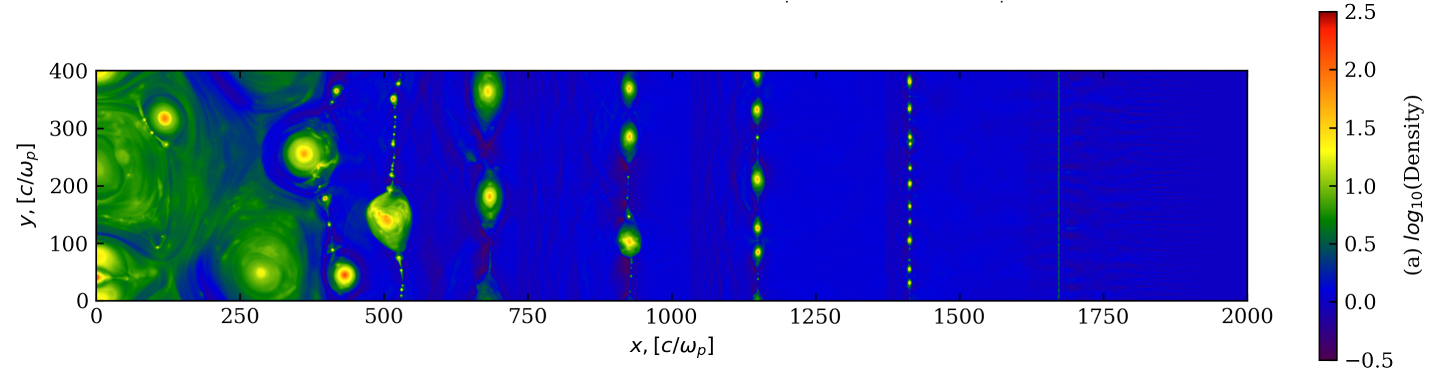
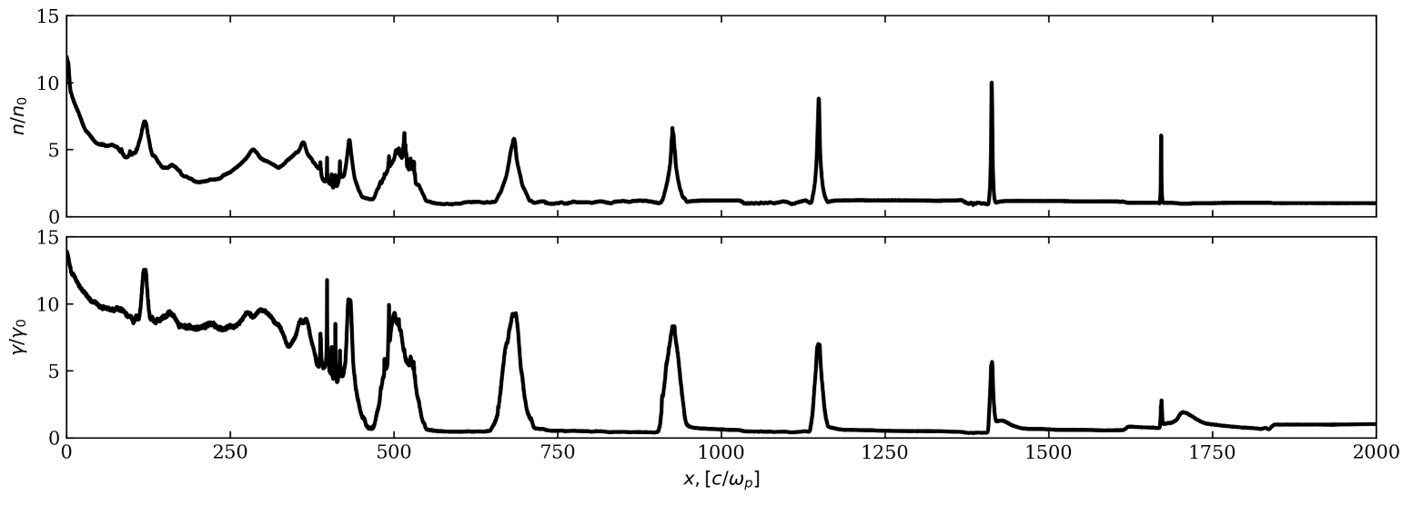
Figure 1: Top: 2D spatial profile of logarithm of particle number density normalized by $n_{c0}$ at time $\omega_{p}t=2000$. Middle: 1D spatial profile (averaged over $y$) of particle number density normalized by $n_{c0}$ at time $\omega_{p}t=2000$. Bottom: 1D spatial profile of average $\gamma$ of all particles normalized by $\gamma_{0}$ at time $\omega_{p}t=2000$.

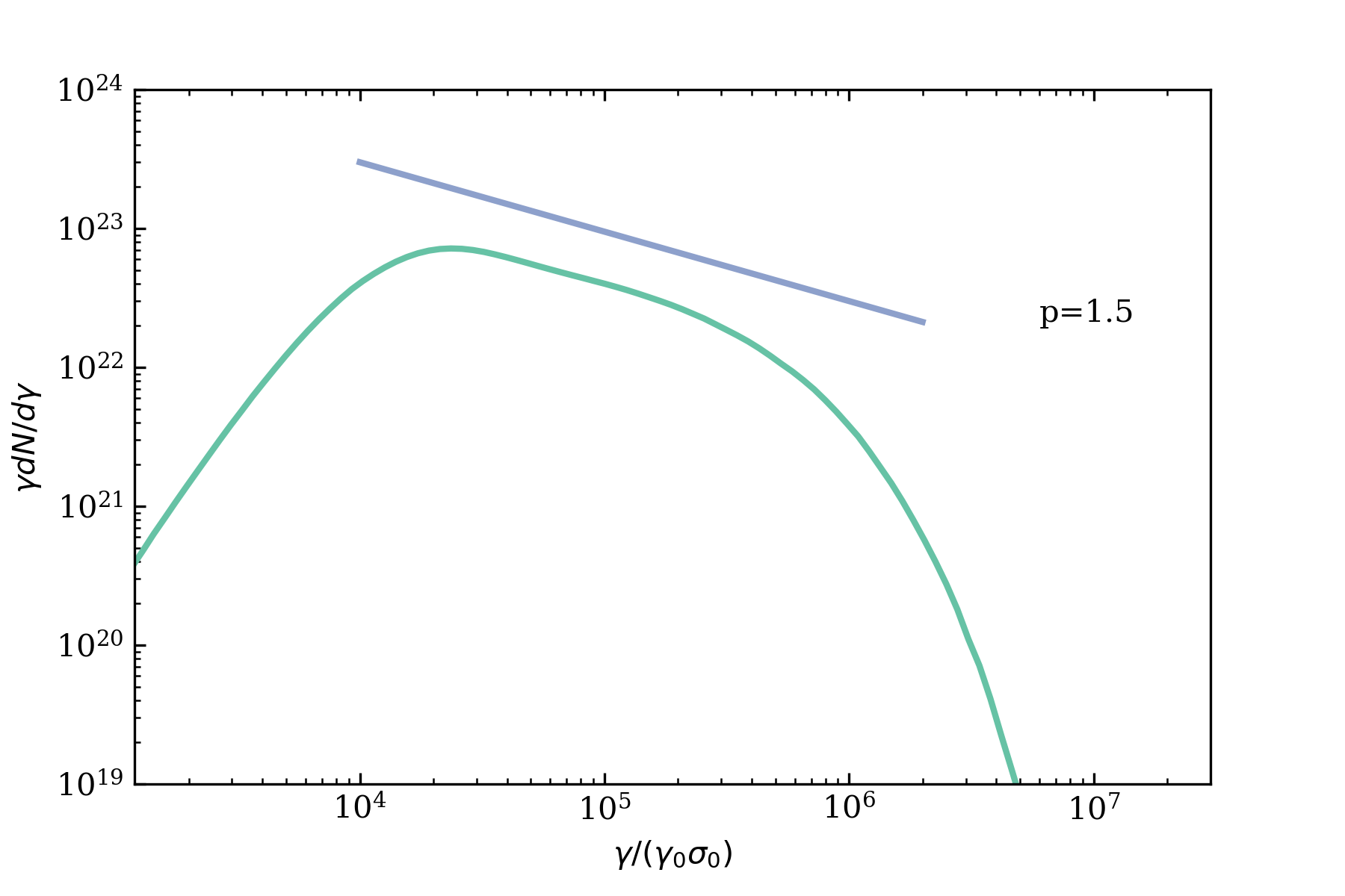
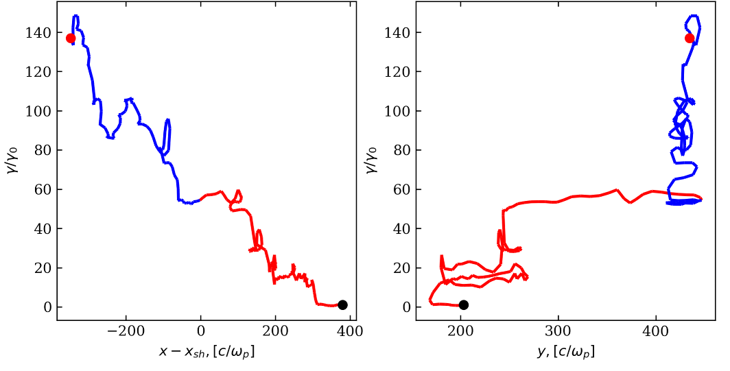
Figure 2: Left: particle energy distribution $\gamma dN/d\gamma$ for all the electrons and positrons in downstream region $0<x<354c/\omega_{p}$ at $\omega_{p}t=2000$. Middle and right: particle trajectory for a particle in the simulation. The middle column is particle Lorentz factor (normalized by $\gamma_{0}$) vs. $x-x_{\mathrm{sh}}$ coordinate where the location of the shock jump is approximately at $x_{\mathrm{sh}}\approx(ct-1000c/\omega_{p})/(2\sqrt{2})$, and the right column is particle Lorentz factor (normalized by $\gamma_{0}$) vs. $y$ coordinate. The red line is the trajectory where the particle is in the upstream, and the red line is the trajectory where the particle is in the downstream. The black dots are for particles at $t=0$, and the red dots are for particles at $\omega_{p}t=2000$.

As shown in Figure 1, the shock forms self-consistently, and propagates to the right side of the simulation box, compresses and decelerates the current sheets. The results are consistent with the previous studySironi2011 . The shock converts the magnetic energy into the particle kinetic energy, resulting in an average particle Lorentz factor $\langle\gamma\rangle\approx\gamma_{0}(1+\sigma_{0})$ in the downstream, which is consistent with the jump condition of ultra-relativistic magnetized shock. The location of the shock is approximately $x_{sh}\approx(ct-1000c/\omega_{p})/(2\sqrt{2})$, moving at speed approximately $c/(2\sqrt{2})$. In the upstream, the current sheets start to continuously break into a series of magnetic islands separated by X-points. The islands coalesce, grow to larger size, and further grow after passing the shock front.

The energy distribution function at downstream of the shock follows a power law $f(\varepsilon)\propto\varepsilon^{-p+1}$ with $p=1.5$ as shown in Figure 2. The trajectory for a typical tracer particle that feels the self-consistent electromagnetic field is shown in Figure 2. The trajectories of most high-energy tracer particles are similar to the one in Figure 2. Those tracer particles (i) bounce several times in the upstream and then travel into the downstream, or (ii) travel into the downstream and bounce several times in the downstream, or (iii) do (i) followed by (ii). Few particles get bounced between upstream and downstream, i.e after a particle travels into the downstream of the shock it rarely travels back into the upstream. The fact that we get a $p=1.5$ power law is consistent with the picture that Fermi mechanism in the reconnection islands is much more efficient than the diffusive shock acceleration.

4 Conclusions and discussions

While a growing body of research using PIC methods focus on the particle acceleration in the spontaneous relativistic magnetic reconnection in the magnetically dominated regime, in this work we extended the study by setting up a simulation with shock driven magnetic reconnection at the termination shock of relativistic striped wind. The analysis shows that many particles are accelerated by Fermi-type mechanism. It is known that PIC simulations only covers a small region in the termination shock, while in reality there is enormous scale separation between the system size and the dynamical scale such as $c/\omega_{p}$. However, to model the particle acceleration during magnetic reconnection in a macroscopic system, it is important to determine the dominant acceleration mechanism.

Research presented in this paper was supported by the Center for Space and Earth Science (CSES) program, Laboratory Directed Research and Development (LDRD) program 20200367ER of Los Alamos National Laboratory (LANL) and NASA ATP program through grant NNH17AE68I. The research by P. K. was also supported by CSES. CSES is funded by LANL’s LDRD program under project number 20180475DR. The simulations were performed with LANL Institutional Computing which is supported by the U.S. Department of Energy National Nuclear Security Administration under Contract No. 89233218CNA000001.

References

- (1) H. Yuksel, M.D. Kistler, T. Stanev, Physical Review Letters 103 (2009)
- (2) M. Amenomori, Y. Bao, X. Bi, D. Chen, T. Chen, W. Chen, X. Chen, Y. Chen, Cirennima, S. Cui et al., Physical Review Letters 123 (2019)
- (3) A.U. Abeysekara, A. Albert, R. Alfaro, C. Alvarez, J.D. Álvarez, J.R.A. Camacho, R. Arceo, J.C. Arteaga-Velázquez, K.P. Arunbabu, D.A. Rojas et al., The Astrophysical Journal 881, 134 (2019)
- (4) A.U. Abeysekara, A. Albert, R. Alfaro, C. Alvarez, J.D. Álvarez, R. Arceo, J.C. Arteaga-Velázquez, D.A. Rojas, H.A.A. Solares, A.S. Barber et al., Science 358, 911 (2017)
- (5) L. Accardo, M. Aguilar, D. Aisa, B. Alpat, A. Alvino, G. Ambrosi, K. Andeen, L. Arruda, N. Attig, P. Azzarello et al., Physical Review Letters 113 (2014)
- (6) D. Hooper, I. Cholis, T. Linden, K. Fang, Physical Review D 96 (2017)
- (7) A.A. Abdo, B. Allen, D. Berley, S. Casanova, C. Chen, D.G. Coyne, B.L. Dingus, R.W. Ellsworth, L. Fleysher, R. Fleysher et al., The Astrophysical Journal 664, L91 (2007)
- (8) T. Linden, B.J. Buckman, Physical Review Letters 120 (2018)
- (9) M.J. Rees, J.E. Gunn, Monthly Notices of the Royal Astronomical Society 167, 1 (1974)
- (10) C.F. Kennel, F.V. Coroniti, The Astrophysical Journal 283, 694 (1984)
- (11) C.F. Kennel, F.V. Coroniti, The Astrophysical Journal 283, 710 (1984)
- (12) F.V. Coroniti, The Astrophysical Journal 349, 538 (1990)
- (13) J.G. Kirk, O. Skjaraasen, The Astrophysical Journal 591, 366 (2003)
- (14) O. Porth, S.S. Komissarov, R. Keppens, Monthly Notices of the Royal Astronomical Society 438, 278 (2014), 1310.2531
- (15) B. Olmi, L.D. Zanna, E. Amato, N. Bucciantini, Monthly Notices of the Royal Astronomical Society 449, 3149 (2015)
- (16) O. Porth, M.J. Vorster, M. Lyutikov, N.E. Engelbrecht, Monthly Notices of the Royal Astronomical Society 460, 4135 (2016)
- (17) L. Sironi, A. Spitkovsky, The Astrophysical Journal 741, 39 (2011)
- (18) G. Giacinti, J.G. Kirk, The Astrophysical Journal 863, 18 (2018)
- (19) J. Pétri, Y. Lyubarsky, Astronomy & Astrophysics 473, 683 (2007)
- (20) L. Sironi, A. Spitkovsky, The Astrophysical Journal 783, L21 (2014)
- (21) F. Guo, H. Li, W. Daughton, Y.H. Liu, Physical Review Letters 113 (2014)
- (22) F. Guo, Y.H. Liu, W. Daughton, H. Li, The Astrophysical Journal 806, 167 (2015)
- (23) G.R. Werner, D.A. Uzdensky, B. Cerutti, K. Nalewajko, M.C. Begelman, The Astrophysical Journal 816, L8 (2015)
- (24) F. Guo, X. Li, W. Daughton, P. Kilian, H. Li, Y.H. Liu, W. Yan, D. Ma, The Astrophysical Journal 879, L23 (2019)
- (25) T.D. Arber, K. Bennett, C.S. Brady, A. Lawrence-Douglas, M.G. Ramsay, N.J. Sircombe, P. Gillies, R.G. Evans, H. Schmitz, A.R. Bell et al., Plasma Physics and Controlled Fusion 57, 113001 (2015)
- (26) Y. Lu, P. Kilian, F. Guo, H. Li, E. Liang (2019), http://arxiv.org/abs/1909.09613v1
- (27) L.D. Landau, E.M. Lifshitz, C.H. Holbrow, Physics Today 16, 72 (1963)