STREAmS: a high-fidelity accelerated solver for direct numerical simulation of compressible turbulent flows

Abstract

We present STREAmS, an in-house high-fidelity solver for large-scale, massively parallel direct numerical simulations (DNS) of compressible turbulent flows on graphical processing units (GPUs). STREAmS is written in the Fortran 90 language and it is tailored to carry out DNS of canonical compressible wall-bounded flows, namely turbulent plane channel, zero-pressure gradient turbulent boundary layer and supersonic oblique shock-wave/boundary layer interactions. The solver incorporates state-of-the-art numerical algorithms, specifically designed to cope with the challenging problems associated with the solution of high-speed turbulent flows and can be used across a wide range of Mach numbers, extending from the low subsonic up to the hypersonic regime. The use of cuf automatic kernels allowed an easy and efficient porting on the GPU architecture minimizing the changes to the original CPU code, which is also maintained. We discuss a memory allocation strategy based on duplicated arrays for host and device which carefully minimizes the memory usage making the solver suitable for large scale computations on the latest GPU cards. Comparison between different CPUs and GPUs architectures strongly favor the latter, and executing the solver on a single NVIDIA Tesla P100 corresponds to using approximately 330 Intel Knights Landing CPU cores. STREAmS shows very good strong scalability and essentially ideal weak scalability up to 2048 GPUs, paving the way to simulations in the genuine high-Reynolds number regime, possibly at friction Reynolds number $Re_{\tau}>10^{4}$. The solver is released open source under GPLv3 license and is available at https://github.com/matteobernardini/STREAmS.

1 Introduction

Compressible flows are ubiquitous in aerospace applications and in recent years there has been a renewed interest in the field, owing to the rising investments in high-speed flight and space exploration. These technological challenges call attention to high-fidelity numerical methods for compressible wall-bounded flows which have proved to be a valuable tool to unveil the complexity of these flows.

The flow physics of compressible wall-bounded turbulence is undoubtedly richer than that of incompressible flows. The hyperbolic nature of the equations allows for the presence of propagating disturbances and discontinuities such as shock waves, which interact with the underlying turbulence, leading to flow phenomena that are absent in the incompressible case. This additional complexity has affected and slowed down the development of numerical methods for compressible flows, as compared to the incompressible ones. Baseline numerical algorithms for direct numerical simulation (DNS) of incompressible flows were mainly developed between the sixties and the eighties ¹, ², ³, ⁴, and basically settled since then. The reliability of these algorithms and the advent of the open-source software promoted the development of several incompressible open-source solvers for fluid dynamics, both multi-purpose solvers as OpenFOAM ⁵, Nek5000 ⁶ and Nektar++ ⁷ and academic solvers as AFiD ⁸ and CaNS ⁹. These solvers are based on central processing units (CPUs) and message passing interface (MPI) parallelization, which has been the standard approach in high-performance computing (HPC) ¹⁰ in the past twenty years. However, in the race towards exascale computing, the HPC architectures are showing consistent trend towards the use of graphical processing units (GPUs). In the last decade, GPUs have become the favorite solution to achieve accelerated cutting-edge performance with high energy efficiency. In particular, in the latest Top500 survey ¹¹, which reports the ranking of the most powerful 500 machines worldwide, 136 machines are NVIDIA GPU-Accelerated ¹² for a total of about $40\%$ of the total power supplied. In addition, NVIDIA GPUs power $90\%$ of the top 30 supercomputers on the Green500 ¹³, a list of HPC systems with high performance and improved energy efficiency. The incompressible DNS community has already benefited from improved computational performance of GPUs, with two available in-house solvers AFiD-GPU ¹⁴ and CaNS-GPU ¹⁵.

Numerical algorithms for compressible flow DNS are less standardized then the incompressible ones, as several formulations of the underlying equations are possible ¹⁶, ¹⁷, each proving numerical advantages depending on the flow physics involved. For this reason fewer CPUs-based open-source compressible flow solvers are available, compared to the incompressible case. Examples include popular multi-purpose open-source packages ⁵, ¹⁸, ¹⁹, ⁷ and OpenSBLI ²⁰, a Python framework for the automated derivation of finite differences solvers both for CPUs and GPUs architectures. Another option is the use of the recent programming paradigm Legion ²¹ which allows to use the same solver on different HPC architectures (including GPUs), without requiring extensive code restructuring. A recent example of compressible flow solver using Legion is HTR ²², designed for hypersonic reacting flows. To our best knowledge, no open-source GPUs-based compressible solver is currently available, and the aim of this work is to fill this gap by adapting our CPUs-based compressible finite differences flow solver to run on multi-GPU clusters. The CPUs solver stems from 20 years experience of our group on compressible wall-bounded flows and has been used to carry out several seminal DNS studies of canonical flows including supersonic boundary layer ²³, ²⁴, shock/boundary layer interaction (SBLI) ²⁵, ²⁶, supersonic roughness-induced transition ²⁷ and supersonic internal flows ²⁸, ²⁹, ³⁰. The solver was already ported to compute unified device architecture (CUDA) ³¹ for the previous generation of GPUs, which required extensive code re-structuring and optimization.

In this work we present STREAmS (Supersonic TuRbulEnt Accelerated navier stokes Solver) a CUDA Fortran version of our compressible flow solver developed and optimized for the latest generation of GPU clusters. We focus on three canonical wall-bounded turbulent flows, namely the supersonic plane channel, the zero-pressure-gradient boundary layer developing over a flat plate and the oblique shock wave/turbulent boundary layer interaction. We discuss the CUDA implementation strategy and we compare the computational performance with the standard CPU implementation and with the incompressible solvers AFiD-GPU and CaNS-GPU.

2 Methodology

STREAmS solves the fully compressible Navier-Stokes equations for a perfect heat-conducting gas

$$\frac{\partial\rho}{\partial t}+\frac{\partial\rho u_{i}}{\partial x_{i}} =0,$$ (1a)

$$\frac{\partial\rho u_{i}}{\partial t}+\frac{\partial\rho u_{i}u_{j}}{\partial x_{j}} =-\frac{\partial p}{\partial x_{i}}+\frac{\partial\sigma_{ij}}{\partial x_{j}}+f\delta_{i1},$$ (1b)

$$\frac{\partial\rho E}{\partial t}+\frac{\partial\rho u_{j}H}{\partial x_{j}} =-\frac{\partial q_{j}}{\partial x_{j}}+\frac{\partial\sigma_{ij}u_{i}}{\partial x_{j}}+fu_{1},$$ (1c)

where $u_{i}$, $i=1,2,3$, is the velocity component in the i-th direction, $\rho$ the density, $p$ the pressure, $E=c_{v}T+u_{i}u_{i}/2$ the total energy per unit mass, and $H=E+p/\rho$ is the total enthalpy. The components of the heat flux vector $q_{j}$ and of the viscous stress tensor $\sigma_{ij}$ are

$$\sigma_{ij}=\mu\left(\frac{\partial u_{i}}{\partial x_{j}}+\frac{\partial u_{j}}{\partial x_{i}}-\frac{2}{3}\frac{\partial u_{k}}{\partial x_{k}}\delta_{ij}\right),$$ (2)

$$q_{j}=-k\frac{\partial T}{\partial x_{j}},$$ (3)

where the dependence of the viscosity coefficient on temperature is accounted for through Sutherland’s law and $k=c_{p}\mu/\mbox{{Pr}}$ is the thermal conductivity, with $\mbox{{Pr}}=0.72$. The forcing term $f$ in equation (1b) is added in the plane channel flow simulations and is evaluated at each time step in order to discretely enforce constant mass-flow-rate in time. The corresponding power spent is added to the right-hand-side of the total energy equation.

2.1 Spatial discretization

The convective terms in the Navier–Stokes equations are discretized using a hybrid energy-conservative shock-capturing scheme in locally conservative form ³². Let us consider the convective flux in one space direction (say $x$)

$$f_{x}=\rho u\varphi,$$ (4)

where $\varphi$ is the transported quantity, namely $\varphi=1$ for the mass equation, $\varphi=u_{j}$ for the momentum equation and $H$ for the total energy equation. The numerical discretization of the streamwise derivative of the flux $f_{x}$ on a uniform mesh with spacing $\Delta x$ relies on the identification of a numerical flux $\hat{f}_{x\,i+1/2}$ defined at the intermediate nodes such that

$$\frac{\partial f_{x}}{\partial x}\bigg{|}_{i}=\frac{1}{\Delta x}\left(\hat{f}_{x,\,i+1/2}-\hat{f}_{x,\,i-1/2}\right).$$ (5)

Figure 1: Sketch of the computational stencil in one space direction.

An energy-conserving numerical flux at the interface $i+1/2$ (figure 1) can be obtained by defining the three-point averaging operator ³²

$$\left(\widetilde{F,G,H}\right)_{i,l}=\frac{1}{8}\left(F_{i}+F_{i+l}\right)\left(G_{i}+G_{i+l}\right)\left(H_{i}+H_{i+l}\right),$$ (6)

and recasting in conservative form the split formulation of the Eulerian fluxes ³³

$$\hat{f}_{x,\,i+1/2}=2\,\sum_{l=1}^{L}a_{l}\sum_{m=0}^{l-1}\left(\widetilde{\rho,u,\varphi}\right)_{i-m,l},$$ (7)

where the $a_{l}$ are the standard coefficients for central finite-difference approximations of the first derivative, yielding order of accuracy $2\,L$. In smooth (shock-free) regions of the flow we use a fourth-order energy-consistent flux (7), which guarantees that the total kinetic energy is discretely conserved in the limit case of inviscid incompressible flow ²⁶. The locally conservative formulation allows straightforward hybridization of the central flux with classical shock-capturing reconstructions. In our case, shock-capturing capabilities rely on the use of Lax-Friedrichs flux vector splitting, whereby the components of the positive and negative characteristic fluxes are reconstructed at the interfaces using a weighted essentially non-oscillatory (WENO) reconstruction ³⁴. To judge on the local smoothness of the numerical solution we rely on a classical shock sensor ³⁵

$$\theta=\max{\left(\frac{-\nabla\cdot{u}}{\sqrt{{\nabla\cdot u}^{2}+{\nabla\times u}^{2}+u_{0}^{2}/L_{0}}},0\right)}\in[0,1],$$ (8)

where $u_{0}$ and $L_{0}$ are suitable velocity and length scales ²³, defined such that $\theta\approx 0$ in smooth zones, and $\theta\approx 1$ in the presence of shocks. The viscous terms are expanded to Laplacian form and also approximated with fourth-order formulas to avoid odd-even decoupling phenomena,

$$\begin{split}\frac{\partial}{\partial x}\left(\mu\frac{\partial u}{\partial x}\bigg{|}_{i}\right)\bigg{|}_{i}=\frac{\partial\mu}{\partial x}\bigg{|}_{i}\frac{\partial u}{\partial x}\bigg{|}_{i}+\mu\frac{\partial^{2}u}{\partial x^{2}}\bigg{|}_{i}=\\ \frac{1}{{\Delta x}^{2}}\sum_{l=-L}^{L}a_{l}^{2}\mu_{i+l}u_{i+l}+\mu_{i}\frac{1}{{\Delta x}^{2}}\sum_{l=-L}^{L}b_{l}u_{i+l},\end{split}$$ (9)

where $b_{l}$ are the finite differences coefficient for the second derivative of order $2\,L$.

2.2 Time integration

A semi-discrete system of ordinary differential equations stems from discretization of the spatial derivatives,

$$\frac{\mathrm{d}\mathbf{w}}{\mathrm{d}t}=\mathbf{R}(\mathbf{w})$$ (10)

where $\mathbf{w}=[\rho,\rho u,\rho v,\rho w,\rho E]$ is the vector of the conservative variables and $\mathbf{R}$ the vector of the residuals. The system is advanced in time using Wray’s three-stage third-order scheme ³⁶,

$$\mathbf{w}^{(\ell+1)}=\mathbf{w}^{(\ell)}+\alpha_{\ell}\Delta t\mathbf{R}^{(\ell-1)}+\beta_{\ell}\Delta t\mathbf{R}^{(\ell)},\quad\ell=0,1,2,$$ (11)

$\mathbf{w}^{(0)}=\mathbf{w}^{n}$, $\mathbf{w}^{n+1}=\mathbf{w}^{(3)}$ and the integration coefficient are $\alpha_{\ell}=(0,17/60,-5/12)$, $\beta_{\ell}=(8/15,5/12,3/4)$.

3 Validation

STREAmS has been tailored to carry out three types of canonical compressible flow configurations, namely supersonic plane channel flow, supersonic boundary layer and shock wave/boundary layer interaction. In the following we validate the solver for these three flows and compare the results to experimental and numerical data available in the literature. We use both Reynolds ($\phi=\overline{\phi}+\phi^{\prime}$) and Favre ($\phi=\widetilde{\phi}+\phi^{\prime\prime}$, $\widetilde{\phi}=\overline{\rho\phi}/\overline{\rho}$) decompositions, where the overline symbol denotes averaging in the homogeneous space directions and in time.

3.1 Supersonic plane channel flow

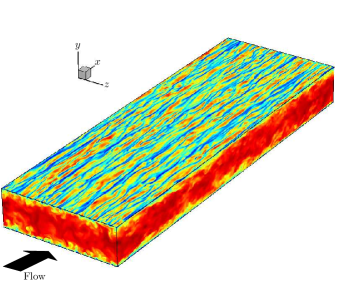
Figure 2: Instantaneous streamwise velocity for plane supersonic channel flow at $\mbox{{Re}}_{\tau}=500$ and $M_{b}=1.5$. The wall-parallel plane is at $y^{+}=15$.

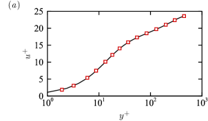
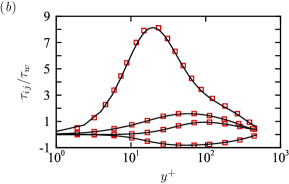
Figure 3: Supersonic plane channel flow at $M_{b}=1.5$ and $\mbox{{Re}}_{\tau}=490$. (a) Mean streamwise velocity profile, $u^{+}=u/u_{\tau}$ as a function of $y^{+}=y/\delta_{v}$. (b) Density scaled turbulent stresses $\tau_{ij}/\tau_{w}$ as a function of $y^{+}$. Present DNS data (black solid) are compared to previous DNS data obtained with the same numerical algorithm ²⁸ (red dashed).

We carry out DNS of plane supersonic channel flow at bulk Mach number $M_{b}=u_{b}/c_{w}=1.5$ and bulk Reynolds number $\mbox{{Re}}_{b}=2\rho_{b}u_{b}h/\mu_{w}=14725$, where $\rho_{b}=1/V\int_{V}\rho\mathrm{d}V$ is the bulk density and $u_{b}=1/(\rho_{b}V)\int_{V}\rho u\mathrm{d}V$ is the bulk velocity in the channel (both exactly constant in time), and $\mu_{w}$ and $c_{w}$ are the dynamic viscosity coefficient and the speed of sound at the wall temperature, respectively. This configuration corresponds to a friction Reynolds number $\mbox{{Re}}_{\tau}=\rho_{w}u_{\tau}h/\mu_{w}=489$, where $u_{\tau}=\sqrt{\tau_{w}/\rho_{w}}$ is the friction velocity and $\tau_{w}$ is the wall shear stress. The computational domain is a rectangular box with size $6\pi h\times 2h\times 2\pi h$ in the $x,y,z$ coordinate directions, respectively and $h$ is the channel half-height. The mesh spacing is constant in the wall-parallel directions, and an error-function mapping is used to cluster mesh points towards the walls. The number of mesh points in the three directions is $N_{x}=1024$, $N_{y}=256$, $N_{z}=512$, corresponding to a mesh spacing in wall units $\Delta x^{+}=9$, $\Delta y^{+}=0.8$–$5.7$ and $\Delta z^{+}=6$. Periodicity is enforced in the homogeneous wall-parallel directions, and no-slip isothermal conditions are imposed at the channel walls. The mesh in the wall-normal direction is staggered such that the wall coincides with an intermediate node, where the convective fluxes are identically zero. This approach guarantees correct telescoping of the numerical fluxes and exact conservation of the total mass, with the further benefit of doubling the maximum allowed time step ²⁸. The simulation is initiated with a parabolic streamwise velocity profile with superposed random perturbations and large-scale sinusoidal perturbations, corresponding to streamwise-aligned rollers. The channel flow simulation is carried out using the central, energy-preserving flux only, as shock waves do not occur in this configuration. Figure 2 shows the instantaneous streamwise velocity in a cross-stream, a streamwise and a wall-parallel plane at $y^{+}=y/\delta_{v}=15$. The instantaneous flow field exhibits the flow organization typical of incompressible wall turbulence, whereby the wall-parallel plane is populated by low- and high-speed streaks associated with sweeps and ejections in the cross-stream plane. Figure 3 shows the mean velocity and Reynolds stress profiles. Excellent agreement between result obtained with STREAmS-GPU and previous DNS carried out with CPU implementation of the solver ²⁸ is found.

3.2 Supersonic turbulent boundary layer

We now consider a spatially-developing zero-pressure-gradient supersonic turbulent boundary layer evolving over a flat plate. A direct numerical simulation is carried out at free-stream Mach number $M_{\infty}=2$ and Reynolds number in the low-moderate regime, up to a momentum thickness Reynolds number $Re_{\delta_{2}}\approx 1900$, corresponding to a friction Reynolds number $Re_{\tau}\approx 600$. As for the case of supersonic channel flow only the energy conservative flux is used as no shock wave discontinuities are present in the flow. To properly capture the large scale structures of the boundary layer (known as superstructures), the simulation is carried out in a long and wide computational box, which extends for $L_{x}=105\delta_{in}$, $L_{y}=12\delta_{in}$, $L_{z}=10\delta_{in}$, in the streamwise (x), wall-normal (y) and spanwise (z) directions, $\delta_{in}$ being the boundary layer thickness at the inflow station, computed considering the $99\%$ of the free-stream velocity. The computational domain is discretized with a mesh consisting of $N_{x}=4096$, $N_{y}=256$, $N_{z}=512$ grid nodes. Uniform mesh spacing is used in the wall-parallel directions, and hyperbolic sine stretching is used in the wall-normal direction to cluster grid points towards to the wall, with wall spacing $\Delta y_{w}^{+}=0.8$. The boundary conditions are specified as follows. At the upper and outflow boundaries non-reflecting boundary conditions are imposed by performing characteristic decomposition in the direction normal to the boundary. Similar characteristic wave treatment is also applied at the no-slip wall boundary, where temperature is set equal to its nominal recovery value $T_{r}/T_{\infty}=1+(\gamma-1)/2\,r\,M_{\infty}^{2}$, with $r=Pr^{1/3}$. In the spanwise direction the flow is assumed to be statistically homogeneous and periodic boundary conditions are applied. A critical issue in the simulation of spatially evolving turbulent flows is the prescription of the inflow turbulence generation method. In STREAmS, velocity fluctuations at the inlet plane are imposed by means of a synthetic digital filtering (DF) approach ³⁷, extended to the compressible case thanks to the use of the strong Reynolds analogy ³⁸. An efficient implementation of the method is achieved using an optimized DF procedure ³⁹, whereby the filtering operation is decomposed in a sequence of fast one-dimensional convolutions. The implementation requires the specification of the Reynolds stress tensor at the inflow plane, which is interpolated by a dataset of previous DNS of supersonic boundary layer performed by the same group ⁴⁰. The computation is initialized by prescribing a mean fully developed turbulent compressible boundary layer obtained by applying the van Driest transformation ⁴¹ to an incompressible profile of the Musker family ⁴².

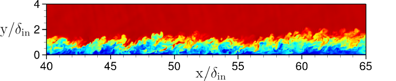
Figure 4: Instantaneous density field in a streamwise wall-normal plane. Contour levels are shown in the range $0.55<\rho/\rho_{\infty}<1.05$.

In figure 4 we show a snapshot of the instantaneous density field in a streamwise wall-normal plane. The figure highlights the main features of the turbulent boundary layer and its multi-scale structure, characterized by an extremely intermittent behavior in the outer layer, with regions of relatively quiescent, high-speed irrotational fluid interspersed with slower, large-scale rotational bulges.

\psfrag{x}[0.8]{$y^{+}$}\psfrag{y}[0.8]{$u_{VD}^{+}$}\includegraphics[width=106.69783pt,angle={270},clip]{./uvd.eps}

\psfrag{x}[0.8]{$y^{+}$}\psfrag{y}[0.8]{$u_{VD}^{+}$}\psfrag{y}[0.8]{$\overline{\rho}\widetilde{u_{i}^{\prime\prime}u_{j}^{\prime\prime}}/\tau_{w}$}\includegraphics[width=106.69783pt,angle={270},clip]{./rey.eps}

Figure 5: Comparison of van-Driest transformed mean streamwise velocity (a) and fluctuating velocity statistics (b) scaled in wall units, with reference incompressible DNS ⁴³, ⁴⁴ data at similar friction Reynolds number. Solid line, present DNS; symbols, reference data. The dashed lines in (a) denote the linear $\overline{u}^{+}=y^{+}$ and log-law $\overline{u}^{+}=5.+2.44\ln y^{+}$.

The distributions of the van Driest transformed mean streamwise velocity profile and velocity fluctuation intensities at a reference station ($x_{\textrm{ref}}=90\delta_{\textrm{in}}$) are reported in figure 5 in inner scaling. The DNS data are compared with the incompressible boundary layer datasets ⁴³, ⁴⁴ at similar friction Reynolds number ($Re\approx 580$). The figure shows near collapse of compressible and incompressible DNS data, after density variations are accounted for.

3.3 Shock-wave/turbulent boundary layer interaction

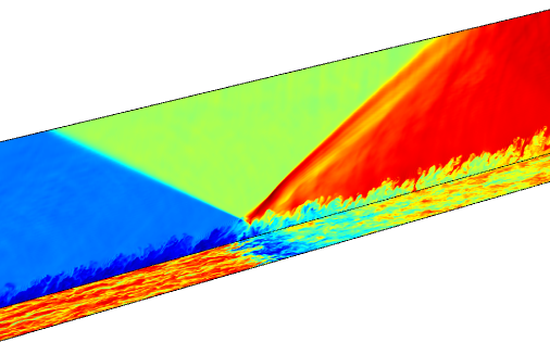
Figure 6: Visualization of main SBLI features. Contours of the instantaneous density field in a streamwise wall-normal plane, superposed with contours of streamwise velocity in a wall-parallel plane at $y^{+}=30$.

\psfrag{x}[t][0.8]{$(x-x_{\textrm{imp}})/L$}\psfrag{y}[b][0.8]{$(\overline{p}_{w}-p_{\infty})/(p_{2}-p_{\infty})$}\includegraphics[width=106.69783pt,angle={270},clip]{./pwall.eps}

\psfrag{x}[t][0.8]{$(x-x_{\textrm{imp}})/L$}\psfrag{y}[b][0.8]{$(\overline{p}_{w}-p_{\infty})/(p_{2}-p_{\infty})$}\psfrag{y}[b][0.8]{$\sqrt{\widetilde{u^{\prime\prime}u^{\prime\prime}}}/u_{\infty}$}\includegraphics[width=106.69783pt,angle={270},clip]{./urms.eps}

Figure 7: Distribution of (a) mean wall pressure and (b) streamwise turbulent fluctuation intensity at $y=0.1L$ as a function of the scaled interaction coordinate $(x-x_{\textrm{imp}})/L$. Solid line, DNS data; open triangles, reference experiment ⁴⁵.

We present a third flow case to test the shock-capturing capabilities of STREAmS. We carry out DNS of shock-wave/turbulent boundary layer interaction to replicate the flow conditions of reference experiments ⁴⁵, characterized by a free-stream Mach number $M=2.28$ and incidence angle of the shock generator $\phi=8^{\circ}$.

The simulation is performed in a computational domain of size $L_{x}\times L_{y}\times L_{z}=[100\times 12\times 6]\delta_{\textrm{in}}$ discretised using $N_{x}\times N_{y}\times N_{z}=[4096\times 384\times 288]$ grid points. Here $\delta_{\textrm{in}}$ represents the thickness of the incoming boundary layer upstream of the interaction. The specification of the boundary condition follows the setup adopted for the previous flow case, except for the upper boundary of the computational domain, where the shock is artificially generated by imposing the inviscid oblique shock solution corresponding to the selected flow deflection.

The flow organization in the investigated SBLI is given by figure 6, where contours of the density field are shown in a streamwise-wall-normal plane superposed with contours of the streamwise velocity fluctuations in a wall-parallel plane. The figure shows the complex structure of the interaction, characterized by the presence of an impinging and a reflected shock, which cause thickening of the incoming boundary layer, and the formation of a small recirculation bubble. The typical pattern of high- and low-speed streaks that characterizes the organization of the streamwise velocity disappears across the interaction region, and reform towards the end of the computational domain, where the boundary layer gradually relaxes to the equilibrium state.

A comparison of DNS data with the reference experiment is reported in Fig  7, where the distribution of the mean wall pressure and of the streamwise fluctuation intensity is shown across the interaction zone, in terms of the scaled interaction coordinate $(x-x_{imp})/L$, $L$ being the distance between the nominal impingement point of the incoming shock and the apparent origin of the reflected shock. It turns out that the structure of the interaction zone is well captured by the simulation, which predicts a wall pressure rise in excellent agreement with the available experimental data. Similarly, very good agreement is observed for the root-mean-square of the streamwise fluctuation intensity, whose increase in the interaction region is associated with the amplification of turbulence caused by the adverse pressure gradient imparted by the shock system.

4 GPU Implementation and computational performance

4.1 Parallelization and GPU porting

HPC is currently facing a major transition as the majority of systems in operation is still based on CPUs, but GPU-based systems are experiencing rapid growth. For this reason in this phase it is very useful to have a code which can be used on different architectures without requiring further modifications. Tuning the code for different architectures typically involves considerable commitment, including management effort in maintaining, updating or modifying multiple versions of the same code. For this reason we design STREAmS to efficiently work on the most common HPC architectures operating today. The code is written in the Fortran language – mostly using Fortran 90 features – which is widely used in HPC, and it is parallelized using the MPI paradigm. Domain decomposition is carried out in two directions – streamwise and spanwise – in order to limit the amount of data transferred for updating the ghost nodes, considering that the communication times may become important when using a large number of tasks.

STREAmS has been developed to support the use of multi-GPUs architectures, while retaining the possibility to compile and use the code on standard CPU based systems. To achieve this goal, different programming approaches are possible. A first option is using directives, for instance OpenACC ⁴⁶ or OpenMP ⁴⁷, which allows to keep the CPU code completely unchanged. A second approach relies on the use of specialized platforms for a specific hardware, which for NVIDIA GPUs are CUDA ⁴⁸ and CUDA-Fortran ⁴⁹. A third strategy is to use more portable but more inconvenient or less popular tools, such as OpenCL ⁵⁰ or HIP: C ++ Heterogeneous-Compute Interface for Portability ⁵¹.

For these reasons in STREAmS we opt for CUDA-Fortran as this allows us to achieve good parallel performance while limiting the changes to the initial CPU code. In particular, the use of the cuf automatic kernels allows the large majority of the code to remain unaltered, thus avoiding keeping different versions of the code. The GPU-specific parts of the solver are marked by the #ifdef USE_CUDA preprocessing directive. This strategy resembles the approach adopted by other popular codes in the field of incompressible turbulence such as AFiD ¹⁴ and CaNS ⁹.

Another important part of the GPU porting is represented by the memory management between CPU and GPU. AFiD employs duplicated arrays residing on host and device, e.g. w and w_gpu, respectively. The device arrays are distinguished using the CUDA Fortran device attribute and are active only when CUDA compilation is enabled, i.e. declared in modules inside preprocessing regions marked by USE_CUDA tokens. When using device variables in the computing procedures, the variables are renamed inside USE_CUDA regions using module aliasing so that the computations can always work with the normal (host) names, i.e. use param, only: w => w_gpu. If the variables are passed, the declaration of the dummy arguments must also be distinguished by adding attributes (device) inside USE_CUDA regions. CaNS instead uses a more recent approach based on CUDA managed memory. The managed memory potentially allows to avoid completely the declaration of the CPU and GPU versions of the same variable that can instead be used both in CPU and GPU code sections. However, the use of managed memory requires particular care to optimize the underlying transfers and to avoid undesired automatic transfers. To achieve a good managed memory implementation, some information must be provided to the CUDA platform, for example through the cudaMemAdvise and cudaMemPrefetchAsync functions, which in our opinion reduce the readability of the code. For this reason in STREAmS we followed a different approach, based on the following strategy. For each array, two versions are declared inside the Fortran module: a baseline array w and the corresponding computing array w_gpu. The latter resides on the device, i.e. has the device attribute, only if the code is compiled by activating CUDA.

real, allocatable, dimension(:,:,:;:) :: w, w_gpu
#ifdef USE_CUDA
attributes(device) :: w_gpu
#endif

Moreover, w_gpu is explicitly allocated only if CUDA compilation is active.

#ifdef USE_CUDA
allocate(w_gpu(1:nx, 1:ny, 1:nz, 5))
#endif

The baseline array w is used during the code initialization and finalization stages while w_gpu is used during the time marching section. To this aim, before starting the time evolution it is necessary to ensure that w_gpu contains the same data as w. If CUDA is active, this is achieved by making a CPU-to-GPU copy managed transparently by CUDA-Fortran. If CUDA is not active, Fortran’s move_alloc procedure is used, which allows to move the allocation from w to w_gpu, both on CPU.

#ifdef USE_CUDA
w_gpu = w
#else
call move_alloc(w, w_gpu)
#endif

A similar procedure is applied for the reverse transfer from GPU to CPU. In conclusion, with this memory management the changes to the original solver are limited to variable declaration and allocation and data transfer between CPU and GPU at the beginning and at the end of the computation, while all the other parts of the code remain mostly unchanged. Specification of the CUDA kernels is done by using automatic cuf syntax,

!$cuf kernel do(3) <<<*,*>>>
 do k=1,nz
  do j=1,ny
   do i=1,nx
    do m=1,nv
     w_gpu(m,i,j,k) = w_gpu(m,i,j,k)+fln_gpu(m,i,j,k)
    enddo
   enddo
  enddo
 enddo
!@cuf iercuda=cudaDeviceSynchronize()

therefore only minor changes to the loops are needed. In particular, interdependent loops have been avoided as well as small loops, which have been converted into scalar variables.

Large computational domains require the use of multiple GPUs, in which each MPI process typically manages one graphic card. Communication between multiple GPUs can be carried out in two main fashions. The first option relies on manual copy between host and GPU to guarantee that the MPI communications always occur between variables residing on the host. The second option relies on the so-called CUDA-Aware MPI implementations which allow the user to call MPI application programming interface (API) passing device-resident variables. STREAmS has been parallelized to support both data communication patterns, selectable according to compilation options. This allows to correctly run in environments where CUDA-Aware implementations are not available. MPI communications between multiple GPUs can negatively affect the parallel performance of the solver, depending on the network speed between the computing nodes. To improve the scalability performance, the GPU implementation of STREAmS optionally supports asynchronous patterns in which the GPU computation is overlapped with the swapping procedure necessary to exchange information across adjacent blocks. This is done by exploiting the built-in asynchrony of the CUDA kernels and the capabilities of the CUDA streams. In this regard, two slightly different strategies were implemented depending on the availability of the CUDA-Aware MPI. As an example, in Figure 8 a sketch of the time-lines corresponding to the evaluation of the streamwise convective fluxes are represented. Basically, the evaluation for internal points can be performed before receiving the ghost nodes and for this reason can be overlapped with MPI communications. Following this idea, the CUDA-Aware MPI implementation (left) is straightforward while the standard MPI implementation (right) requires asynchronous CPU-GPU transfers using cudaMemcpyAsync in a specific CUDA stream. After receiving the data on ghost nodes, the boundary values can be computed.

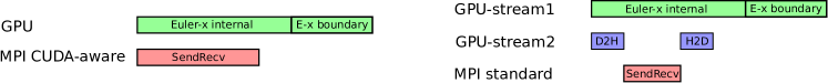
Figure 8: Sketch of asynchronous time-lines for the evaluation of convective fluxes: internal fluxes evaluation (Euler-x internal), boundary fluxes evaluation (E-x boundary), host-to-device transfers (H2D), device-to-host transfers (D2H), MPI communications (SendRecv). CUDA-Aware MPI based time-line is shown on the left while standard MPI time-line is provided on the right.

4.2 Performance results

In this section we discuss the parallel performance of STREAmS, reporting both weak and strong scaling of the code. We have carried out test runs at CINECA on the HPC cluster DAVIDE, an energy-aware Petaflops Class High Performance Cluster based on Power 8 Architecture and coupled with NVIDIA Tesla Pascal GPUs P100 with NVLink. We first report the STREAmS performance on a single GPU card, comparing the elapsed time per time step to a single CPU node, for different HPC architectures, figure 9. For the CPU version of the code, we use the Intel compiler. For this test we use a computational mesh with $1008\times 251\times 234$, corresponding to about 10GB of memory allocation on a GPU. On the top axis figure 9 we report the release dates for each processing unit, highlighting that GPUs present a more significant improvement over the years with respect to CPUs.

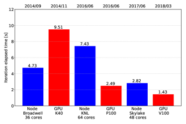
Figure 9: Comparison of STREAmS performance – elapsed time per iteration vs – using different HPC architectures: elapsed time per iteration versus the used processing unit is provided. For CPU-based runs a single computing node is employed using the MPI parallelization. For GPU-based runs a single GPU is used. The grid size is 1008$\times$251$\times$234 (1008$\times$251$\times$236 for KNL run). Improvement of processing unit power over years is underlined by the release dates in the upper horizontal axis.

As for the solver performance on multiple nodes/GPUs we note that communications between GPUs could result in lower performance compared to CPUs, due to the additional data transfer between CPU and GPU. On the other hand, this additional computational cost is typically mitigated due to the use of fewer MPI processes when running on GPUs with respect to CPUs. Figure 10 shows the speed-up of the synchronous and asynchronous versions of the code keeping constant the number of grid points $2560\times 251\times 512$ and using 4 GPUs (one computing node) as reference. Two additional speed-up curves are also reported, corresponding to artificially reduced performance of the interconnection. Low-performance interconnection was emulated by intentionally reiterating the MPI communications seven times. CUDA-Aware MPI was used.

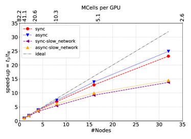
Figure 10: Strong scaling of STREAmS using GPU P100 based cluster D.A.V.I.D.E.: the speed-up of execution compared to the reference case is plotted against the number of used nodes. The grid size is 2560$\times$251$\times$512. The reference case employs one computational node equipped with 4 GPUs. On the upper horizontal axis the millions of cells residing on each GPU is provided to understand the link between the GPU filling and the performances. Four types of MPI parallelization are considered: synchronous, asynchronous, synchronous with artificially slow network and asynchronous with artificially slow network.

Strong scalability is very good up to 4 computing nodes (16 GPUs) and good up to 16 nodes. After that, the speed-up still increases but efficiency degradation is significant. We find that for both network conditions the asynchronous version of the code is slightly faster than the regular one. On the top axis we report the millions of cells processed by each GPU which shows that 10 millions points per GPU are a reasonable threshold to guarantee optimal efficiency.

In Figure 11 we provide a measure of the weak-scaling performance, i.e. by keeping constant the number of cells processed by each GPU. The reference case has again a mesh with $2560\times 251\times 512$ points, but the grid is scaled as the number of nodes increases. We report the number of cells updated per second and per GPU, which should be constant when increasing the total number of GPUs. The performance of the synchronous and asynchronous version of the solver for the case with the real (fast) network are both excellent. In the case of artificially slow network, the synchronous version shows performance degradation, whereas the asynchronous code completely hides the communication times. It may be concluded that using the asynchronous version of the code is always recommended, although the performance improvement is not always significant.

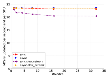
Figure 11: Weak scaling of STREAmS using the GPU P100 based cluster D.A.V.I.D.E.: the millions of cells processed by each GPU per second are plotted against the number of computing nodes. Four types of MPI parallelizations are considered: synchronous, asynchronous, synchronous with artificially slow network and asynchronous with artificially slow network.

Given the availability of recently developed GPU solver for the simulation of canonical incompressible turbulent flows, i.e. AFiD and CaNS, it is interesting to attempt a comparison with the STREAmS performance. The comparison is physically significant in the low-Mach-number limit (say $M_{\infty}<0.2$), at which the results of incompressible and compressible solvers are basically identical ⁵². Obviously, compressible solvers require the evaluation of a much more complex right-hand side and use of smaller time step owing to the acoustic time step restriction. On the other hand, incompressible solvers requires the solution of a Poisson equation at each time step, which is the most computation-intensive part of the solver, implying extensive use of all-to-all MPI communications. AFiD solves the incompressible Navier-Stokes equations with the Boussinesq approximation for temperature with implicit treatment of the diffusive terms. CaNS solves the incompressible equations without the scalar equation, and can be compiled with explicit or implicit treatment of the diffusive terms. The measured clock times per iteration of STREAmS, AFiD and CaNS are compared in Table 1, in a weak scaling test with base computational mesh of 8.39 million of points, and with up to 2048 GPUs. The benchmarks were performed using the CSCS Piz-Daint cluster featuring one P100 GPU per node. Asynchronous standard MPI compilation of STREAmS was employed.

# GPUs	1	2	8	32	128	512	2048
STREAmS	3.65	3.65	3.65	3.65	3.65	3.65	3.65
AFiD	0.84	1.59	1.76	2.17	3.19	5.5	6
CaNS	0.36	1.67	2.1	1.37	1.8	2.34	-

Table 1: Performances of STREAmS compared to popular CFD CUDA-enabled codes AFiD and CaNS. Seven computational grids are provided in the weak scaling spirit starting from 8.39 million grid points case. Correspondingly, the number of employed GPUs ranges from 1 to 2048. For CaNS, explicit compilation for diffusive terms is considered.

Although actual code comparison should also consider the accuracy of the numerical methods needed to achieve equivalent results, it is possible to attempt an interpretation of the trends. First it is observed that, when using a small number of GPUs, the time required by STREAmS for single iteration is larger that for AFiD and for the explicit version of CaNS. On the other hand, since STREAmS shows nearly ideal weak scalability, the performance gap with the incompressible solvers is reduced as the number of GPUs increases, eventually reversing for the AFiD implicit diffusion code. Albeit in a limited and partial context, and depending on the Mach number, this trend suggests that compressible solvers can potentially become competitive with classical incompressible solvers in massively parallel calculations on HPC platforms with thousands of GPUs.

5 Conclusions

We heve presented a recent version of our in-house compressible flow solver STREAmS, that has been been ported to CUDA-Fortran and tailored to canonical wall-bounded flows, namely compressible channel, supersonic boundary layer and SBLI. STREAmS stems from two decades experience of our research group on DNS of compressible wall-bounded flows and a baseline version of the solver, is released open-source under GPLv3 license with the aim to provide the fluid dynamics community with a highly-parallel compressible flow solver. The use of CUDA-Fortran with the use of cuf automatic kernels allowed us to largely minimize the changes to the original flow solver and to compile and run the code on different HPC architectures. The tests carried out on the GPU cluster DAVIDE at CINECA show very good scalability performance, proving that the solver can be used to carry out large scale direct numerical simulations. Interestingly STREAmS shows improved weak scalability performance compared to the state-of-the-art incompressible GPU solvers. Although it is well known that compressible flow solvers typically show better scalability than the incompressible ones, in our experience the difference in performance is less marked on CPUs. This preliminary results show that for large scale simulations using thousands of GPUs the use of compressible flow solvers operating at low Mach number could potentially become competitive with incompressible solvers, despite the substantial overhead in terms of floating point operations, and the restriction on the acoustic time step limitation.

The availability of the GPU version of the solver will allow to take advantage of the contemporary pre-Exascale systems and the next generation of Exascale supercomputers currently under development, allowing to significantly extend the range of simulated Reynolds number up to the genuine high-Reynolds number regime ($Re_{\tau}>10^{4}$). This opportunity will allow the flow community to provide definite answers to key issues, as the presence of a logarithmic range of variation of the streamwise velocity variance with the wall distance, as predicted in the overlap layer by the attached eddy hypothesis, and for which partial support comes from high-Reynolds-number experiments.

Acknowledgements
M. Bernardini was supported by the Scientific Independence of Young Researchers program 2014 (Active Control of Shock-Wave/ Boundary-Layer Interactions project, grant RBSI14TKWU), which is funded by the Ministero Istruzione Università e Ricerca. The authors are especially grateful for the computational resources provided by the Cineca Italian Computing Center.

References

- (1) G. Patterson, S. Orszag, Spectral calculations of isotropic turbulence: Efficient removal of aliasing interactions, Phys. Fluids 14 (11) (1971) 2538–2541.
- (2) J. Kim, P. Moin, R. Moser, Turbulence statistics in fully developed channel flow at low Reynolds number, J. Fluid Mech. 177 (1987) 133–166.
- (3) F. Harlow, J. Welch, Numerical calculation of time-dependent viscous incompressible flow of fluid with free surface, Phys. Fluids 8 (12) (1965) 2182–2189.
- (4) P. Orlandi, Fluid flow phenomena: a numerical toolkit, Vol. 55, Springer Science & Business Media, 2012.
- (5) H. Weller, G. Tabor, H. Jasak, C. Fureby, A tensorial approach to computational continuum mechanics using object-oriented techniques, Comput. Phys. 12 (6) (1998) 620–631.
-
(6)
P. Fisher, J. Kruse, J. Mullen, H. Tufo, J. Lottes, S. Kerkemeier,
NEK5000: open source
spectral element CFD solver (2008).
URL http://nek5000.mcs.anl.gov/index.php/MainPage - (7) C. Cantwell, D. Moxey, A. Comerford, A. Bolis, G. Rocco, G. Mengaldo, D. D. Grazia, S. Yakovlev, J.-E. Lombard, D. Ekelschot, B. Jordi, H. Hu, Y. Mohamied, C. Eskilsson, B. Nelson, P. Vos, C. Biotto, R. Kirby, S. Sherwin, Nektar++: An open-source spectral/hp element framework, Comput. Phys. Commun. 192 (2015) 205–219.
- (8) E. van der Poel, R. Ostilla-Mónico, J. Donners, R. Verzicco, A pencil distributed finite difference code for strongly turbulent wall-bounded flows, Comput. Fluids 116 (2015) 10–16.
- (9) P. Costa, A FFT-based finite-difference solver for massively-parallel direct numerical simulations of turbulent flows, Comput. Math. Appl. 76 (8) (2018) 1853–1862.
- (10) V. Lee, C. Kim, J. Chhugani, M. Deisher, D. Kim, A. Nguyen, N. Satish, M. Smelyanskiy, S. Chennupaty, P. Hammarlund, R. Singhal, P. Dubey, Debunking the 100X GPU vs. CPU myth: an evaluation of throughput computing on CPU and GPU, in: ISCA ‘10: proceedings of the 37th annual international symposium on computer architecture. New York, NY, USA, Vol. 38, ACM, 2010, pp. 451–460.
-
(11)
J. Dongarra, P. Luszczek,
TOP500, Springer US,
Boston, MA, 2011.
doi:10.1007/978-0-387-09766-4_157.
URL https://doi.org/10.1007/978-0-387-09766-4_157 - (12) 136 GPU-Accelerated Supercomputers Feature in TOP500 | NVIDIA Blog, https://blogs.nvidia.com/blog/2019/11/19/record-gpu-accelerated-supercomputers-top500/, accessed: 2020-01-16.
- (13) The GREEN 500, https://www.top500.org/green500/, accessed: 2020-01-16.
- (14) X. Zhu, E. Phillips, V. Spandan, J. Donners, G. Ruetsch, J. Romero, R. Ostilla-Mónico, Y. Yang, D. Lohse, R. Verzicco, M. Fatica, R. Stevens, AFiD-GPU: a versatile Navier–Stokes solver for wall-bounded turbulent flows on GPU clusters, Comput. Phys. Commun 229 (2018) 199–210.
- (15) P. Costa, E. Phillips, L. Brandt, M. Fatica, GPU acceleration of CaNS for massively-parallel direct numerical simulations of canonical fluid flows, arXiv preprint arXiv:2001.05234.
- (16) A. Honein, P. Moin, Higher entropy conservation and numerical stability of compressible turbulence simulations, J. Comput. Phys. 201 (2) (2004) 531–545.
- (17) G. Coppola, F. Capuano, S. Pirozzoli, L. de Luca, Numerically stable formulations of convective terms for turbulent compressible flows, J. Comput. Phys. 382 (2019) 86–104.
- (18) D. Modesti, S. Pirozzoli, A low-dissipative solver for turbulent compressible flows on unstructured meshes, with OpenFOAM implementation, Comput. Fluids 152 (2017) 14–23.
- (19) T. Economon, F. Palacios, S. Copeland, T. Lukaczyk, J. Alonso, SU2: An open-source suite for multiphysics simulation and design, AIAA Journal 54 (3) (2015) 828–846.
- (20) C. Jacobs, S. Jammy, N. Sandham, OpenSBLI: A framework for the automated derivation and parallel execution of finite difference solvers on a range of computer architectures, J. Comput. Sci. 18 (2017) 12–23.
- (21) Legion webpage, https://legion.stanford.edu/, accessed: 2020-03-313131.
- (22) M. D. Renzo, L. Fu, J. Urzay, HTR solver: An open-source exascale-oriented task-based multi-GPU high-order code for hypersonic aerothermodynamics, Comput. Phys. Commun. (2020) 107262.
- (23) S. Pirozzoli, M. Bernardini, Turbulence in supersonic boundary layers at moderate Reynolds number, J. Fluid Mech. 688 (2011) 120–168.
- (24) S. Pirozzoli, M. Bernardini, Probing high-Reynolds-number effects in numerical boundary layers, Phys. Fluids 25 (2) (2013) 021704.
- (25) S. Pirozzoli, F. Grasso, Direct numerical simulation of impinging shock wave/turbulent boundary layer interaction at M, Phys. Fluids 18 (6) (2006) 065113.
- (26) S. Pirozzoli, M. Bernardini, F. Grasso, Direct numerical simulation of transonic shock/boundary layer interaction under conditions of incipient separation, J. Fluid Mech. 657 (2010) 361–393.
- (27) M. Bernardini, S. Pirozzoli, P. Orlandi, Compressibility effects on roughness-induced boundary layer transition, Int. J. Heat and Fluid Flow 35 (2012) 45–51.
- (28) D. Modesti, S. Pirozzoli, Reynolds and Mach number effects in compressible turbulent channel flow, Int. J. Heat Fluid Flow 59 (2016) 33–49.
- (29) D. Modesti, S. Pirozzoli, Direct numerical simulation of supersonic pipe flow at moderate Reynolds number, Int. J. Heat Fluid Flow 76 (2019) 100–112.
- (30) D. Modesti, S. Pirozzoli, F. Grasso, Direct numerical simulation of developed compressible flow in square ducts, Int. J. Heat Fluid Flow 76 (2019) 130–140.
- (31) F. Salvadore, M. Bernardini, M. Botti, GPU accelerated flow solver for direct numerical simulation of turbulent flows, J. Comput. Phys. 235 (2013) 129–142.
- (32) S. Pirozzoli, Generalized conservative approximations of split convective derivative operators, J. Comput. Phys. 229 (19) (2010) 7180–7190.
- (33) C. Kennedy, A. Gruber, Reduced aliasing formulations of the convective terms within the Navier-Stokes equations for a compressible fluid, J. Comput. Phys. 227 (3) (2008) 1676–1700.
- (34) G. S. Jiang, C. W. Shu, Efficient implementation of weighted eno schemes, J. Comput. Phys. 126 (1996) 202.
- (35) F. Ducros, V. Ferrand, F. Nicoud, C. Weber, D. Darracq, D. Gacherieu, T. Poinsot, Large-eddy simulation of the shock/turbulence interaction, J. Comput. Phys. 152 (2) (1999) 517–549.
- (36) P. Spalart, R. Moser, M. Rogers, Spectral methods for the Navier-Stokes equations with one infinite and two periodic directions, J. Comput. Phys. 96 (2) (1991) 297–324.
- (37) M. Klein, A. Sadiki, J. Janicka, A digital filter based generation of inflow data for spatially developing direct numerical or large eddy simulations, J. Comput. Phys. 186 (2) (2003) 652–665.
- (38) E. Touber, N. D. Sandham, Large-eddy simulation of low-frequency unsteadiness in a turbulent shock-induced separation bubble., Theoretical and Computational Fluid Dynamics 23 (2009) 79–107.
- (39) A. Kempf, S. Wysocki, M. Pettit, An efficient, parallel low-storage implementation of Klein’s turbulence generator for les and dns, Computers & fluids 60 (2012) 58–60.
- (40) S. Pirozzoli, M. Bernardini, Supersonic turbulent boundary layers - DNS database, http://newton.dma.uniroma1.it/dnsm2 (2011).
- (41) S. A.J., J. Dussauge, Turbulent Shear Layers in Supersonic Flow, American Institute of Physics, New York, 2006.
- (42) E. expression for the smooth wall velocity distribution in a turbulent boundary layer, Musker, a.j., AIAA J. 17 (1979) 655–657.
- (43) M. Simens, J. Jimenez, S. Hoyas, Y. Mizuno, A high-resolution code for turbulent boundary layers, J. Comput. Phys. 228 (2009) 4218–4231.
- (44) J. Jimenez, S. Hoyas, M. Simens, Y. Mizuno, Turbulent boundary layers and channels at moderate Reynolds numbers, J. Fluid Mech. 657 (2010) 335–360.
- (45) P. Dupont, C. Haddad, J. Debiéve, Space and time organization in a shock-induced separated boundary layer, J. Fluid Mech. 559 (2006) 255–277.
- (46) OpenACC, https://www.openacc.org/, accessed: 2020-01-16.
- (47) OpenMP, https://www.openmp.org/, accessed: 2020-01-16.
- (48) CUDA, https://developer.nvidia.com/cuda-zone, accessed: 2020-01-16.
- (49) CUDA FORTRAN, https://developer.nvidia.com/cuda-fortran, accessed: 2020-01-16.
- (50) OpenCL, https://www.khronos.org/opencl/, accessed: 2020-01-16.
- (51) HIP : C++ Heterogeneous-Compute Interface for Portability, https://gpuopen.com/compute-product/hip-convert-cuda-to-portable-c-code/, accessed: 2020-01-16.
- (52) D. Modesti, S. Pirozzoli, An efficient semi-implicit solver for direct numerical simulation of compressible flows at all speeds, J. Sci. Comput. 75 (2018) 308–331.