Random walkers on a deformable medium

Abstract

We consider random walkers that deform the medium as they move, enabling a faster motion in regions which have been recently visited. This induces an effective attraction between walkers mediated by the medium, which can be regarded as a space metric, giving rise to a statistical mechanics toy model either for gravity, motion through deformable matter or adaptable geometry. In the strong-deformability regime, we find that diffusion is initially described by the porous medium equation, thus yielding subdiffusive behavior of an initially localized cloud of particles. Indeed, while the average width of a single cloud will sustain a $\sigma\sim t^{1/2}$ growth, the combined width of the whole ensemble will grow like $\sigma\sim t^{1/3}$ in a certain time regime. This difference can be accounted for by the strong correlations between the particles, which we explore indirectly through the fluctuations of the center of mass of the cloud and the expected value of the experienced density, defined as the average density measured by the particles themselves.

I Introduction

Let us consider random walkers in a forest leaving some trail behind them, which they may come across again at a later time. The walkers may then choose to avoid that trail or, otherwise, be attracted towards it. Thus, the walkers interact with the medium, which will interact with the walkers in its turn. Alternatively, we may consider the walkers to have a memory of past events, changing their behavior appropriately.

Random walkers with a memory, which are also called non-Markovian, have been described thoroughly. Specially interesting is the elephant random walk (ERW), in which the random walker copies the step taken some random time ago note_erw ; schutz.04 ; kumar.10 ; dasilva.14 ; kearney.18 . Random walkers can be interpreted as foragers gathering food, and in that case they may decide from time to time to jump to a previous point in their search path, where they were specially successful. This gives rise to the random walks with relocation boyer.14 ; boyer.14.2 ; boyer.16 , which are very useful to describe animal motion, and to develop search algorithms campos.15 ; falcon.17 .

Self-avoiding walks, on the other hand, were developed in the context of polymer science degennes.79 . The walk is assigned a probability globally, not step-by-step, which becomes zero when the walk intersects itself amit.83 . Alternatively, random walkers can be either forbidden to cross their previous path, thus allowing them to become trapped, or they may receive an energy penalty for each self-cross domb.72 ; stanley.83 .

Yet, random walkers may present an affinity towards already visited sites, as it is the case with taxis in biology othmer.97 ; permantle.07 , forming reinforced random-walks where the walker finds it more likely to step on an already visited site, with memory sometimes fading with time, often to the extreme of only remembering the last step davis.90 ; sapozhnikov.94 ; ordemann.01 ; foster.09 . Random walkers may also create a potential well around the visited sites, thus energetically encouraging future visits huang.02 ; tan.02 . Moreover, they may interact by leaving a tracing chemical substance, in the process known as chemotaxis Schweitzer.19 . Such reinforced random-walks may present lack of self-averaging and give rise to interesting open problems, such as the determination of the trapping probability kozma.12 . Similar ideas have been successfully applied to the design of optimization algorithms on complex landscapes, such as the ant colony optimizationant_colony or the river formation heuristicsriver_formation .

In this work we consider random walkers that reduce the waiting time associated with a link each time they traverse it miyazama.87 ; bouchaud.90 ; li.17 . This can be considered equivalent to a change in the local speed of light or, in other words, a deformation in the space-time metric. Thus, walkers move faster in regions which have been recently visited. Yet, we will consider the metric to present a tendency to return to its undeformed state when the walkers are not disturbing it. Interestingly, the random walkers will feel an effective attraction mediated by the metric deformations, giving rise to strongly correlated clusters which suggest that the system may serve as a toy model for stochastic gravity hu.04 .

In the continuum limit, the position-dependent waiting times map to an inhomogeneous diffusivity. Thus, we can write a generalized diffusion equation with two fields: matter is described by the probability distribution for the walker positions, and the medium or geometry is described by the diffusivity field. The associated partial differential equations are non-linear, and in the strong coupling limit we will show that they are ruled by the porous medium equation vazquez.91 , with non-trivial scaling exponents showing subdiffusive behavior.

This article is organized as follows. Section II describes our discrete 1D random-walk model on a deformable medium (RWDM). The continuum limit of this model is considered in Sec. III, which discusses the expected scaling properties. Extensive numerical simulations are performed and discussed in Sec. IV, which give rise to a physical picture which is discussed in Sec. V. Sec. VI provides a summary of the conclusions and proposals for further work.

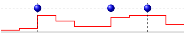
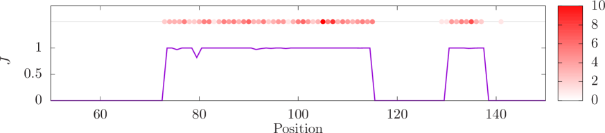
Figure 1: Top: Illustration of the RWDM model. Walkers are represented by the balls, while the hopping probabilities between neighboring sites are represented by the red line. Bottom: A configuration for ${\cal J}_{0}=10^{-6}$, ${\cal J}_{1}=1$, $t_{0}=10$ and $N_{P}=200$ particles on $L=200$ sites, after $T=10^{8}$ time-steps. The purple line denotes the hopping probabilities, red balls represent the positions of the particles, and the color intensity denotes the number of particles at a certain site. Notice that most hopping probabilities are near ${\cal J}_{0}$ or ${\cal J}_{1}$, and that the particles are neatly divided into two blocks.

II Random-Walk on Deformable Medium

Let us describe our model, which will be called the random walk on a deformable medium (RWDM). We consider $N_{P}$ random walkers on a chain. When a walker is standing on site $i$, it has a certain probability per unit time $J_{i,i-1}$ of hopping towards site $i-1$, and $J_{i,i+1}$ of hopping towards site $i+1$. We will assume that probabilities are symmetric, i.e. $J_{i,i+1}=J_{i+1,i}$, and we will introduce the convenient notation $J_{i}\equiv J_{i,i+1}$. The set of $\{J_{p}\}$ values will be called the medium or the metric. Notice that the hopping process on a single link follows a Poissonian law, and that the expected waiting time before hopping is inversely proportional to the hopping rate. Thus, the walker may take either its left link with hopping rate $J_{i-1}$ or its right link with hopping rate $J_{i}$. The top panel of Fig. 1 provides an illustration.

The $N_{P}$ particles are initially placed at the center of a size $L$ chain with periodic boundaries and all hopping probabilities $J_{i}={\cal J}_{0}$ numerical . A suitable time-step is chosen, $\Delta t$. At each turn, we select a random particle and look up its location, $i$. We decide whether to attempt a jump to the left or to the right with equal probabilities. The jump attempt will succeed with probability $P=J_{k}\Delta t$, where $k=i-1$ for a left jump, or $k=i$ for a right jump. After a successful jump attempt, the link will increase its hopping probability according to the rule

$$J_{k}\to J_{k}+{\Delta t\over t_{0}}\left({\cal J}_{1}-J_{k}\right),$$ (1)

where ${\cal J}_{1}\geq{\cal J}_{0}$, thus completing the turn. After a round of $N_{P}$ turns, we assert that time has advanced by a time-step $\Delta t$. Then, all links which have not been updated during this round are subject to the relaxation rule,

$$J_{k}\to J_{k}-{\Delta t\over t_{0}}\left(J_{k}-{\cal J}_{0}\right).$$ (2)

Notice that, in the continuum limit, rules (1) and (2) correspond respectively to an exponential increase or decrease towards the maximum and minimum values, ${\cal J}_{1}$ and ${\cal J}_{0}$, with the same characteristic time $t_{0}$. A typical configuration after a long simulation time can be seen in the bottom panel of Fig. 1.

If ${\cal J}_{1}={\cal J}_{0}$, the metric becomes rigid and the particles will follow a standard random walk. Thus, in this limit we expect that the particle cloud will behave diffusively, i.e. the expected deviation of the particle positions will scale like $\sigma\sim t^{1/2}$. If ${\cal J}_{1}>{\cal J}_{0}$ then the particles will present a trend to hop on already used links, thus spending more time on the regions already visited. This may lead to self-localization of the particle cloud, through interaction with the medium. In this case, we may still expect a power-law behavior, with the traversed distance growing like $t^{\alpha}$ and $\alpha<1/2$.

Our model can be considered as a type of reinforced random walk model, and as such it may show absence of self-averaging. Yet, our system presents an important difference. In a typical reinforced random walk model particles are more likely to jump on sites already visited davis.90 , sometimes through an energy advantage huang.02 ; tan.02 . In our model the medium is deformed through a change in the hopping rates. Sites do not attract particles, instead they move faster through recently visited regions.

Fig. 2 (a) shows two histories, using $\Delta t=1$, $t_{0}=10$, ${\cal J}_{0}=10^{-6}$ and ${\cal J}_{1}=1$ on a $L=200$ chain with $N_{P}=200$ particles. The X-axis represents time in logarithmic scale, while the Y-axis represents the position. Color intensity denotes the hopping probabilities $J_{i}$, where we can see that most values are close to either ${\cal J}_{0}$ or ${\cal J}_{1}$. The width of the cloud at a certain time can be estimated from the vertical range of the high hopping region, ${\cal H}\equiv\{i|J_{i}\approx{\cal J}_{1}\}$. Indeed, the cloud stays localized at the center up to times of order $\approx 3000$. Afterwards, it increases its width for some time, and then either opens up (top) or drifts laterally (bottom). Two trajectories of individual particles have been traced, showing that the walkers spread all over the high-hopping region.

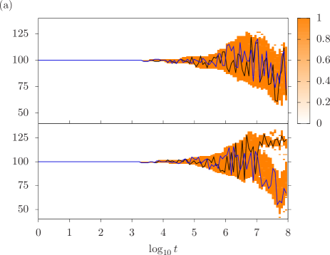
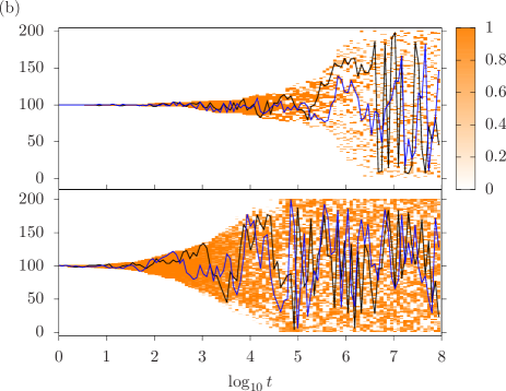
Figure 2: (a) Two system histories, using $N_{P}=200$ particles, ${\cal J}_{0}=10^{-6}$, ${\cal J}_{1}=1$, $t_{0}=10$ and $L=200$. Time is represented in the horizontal axis, in logarithmic scale, while the Y-axis stands for positions along the chain. Color denotes the local hopping probability, and two particle histories (out of $N_{P}=200$) are depicted with continuous lines. (b) Similar results using ${\cal J}_{0}=10^{-4}$ (top) and ${\cal J}_{0}=10^{-2}$ (bottom). Notice that larger values of ${\cal J}_{0}$ give rise to sparse distributions of the particle cloud.

Fig. 2 (b) shows the same data for ${\cal J}_{0}=10^{-4}$ (top) and ${\cal J}_{0}=10^{-2}$ (bottom). Notice that the clouds are much more sparse, suggesting that the particles do not constitute a compact cluster in this case.

III Mean-field Continuum description

In order to determine the macroscopic behavior of our model, we will assume that matter can be described through a density function, $P(x,t)$, such that the expected number of particles in a region ${\cal A}$ will be given by

$$\left<N_{\cal A}(t)\right>=N_{P}\int_{\cal A}dx\;P(x,t).$$ (3)

where $P(x,t)$ will be assumed to be smooth. Moreover, the hopping terms will be described by a smooth function too, $J(x,t)$, which we will call the metric field.

The evolution of the density function will be ruled by a diffusion equation through an inhomogeneous medium vazquez.91

$$\partial_{t}P(x,t)=\partial_{x}\Big{(}J(x,t)\partial_{x}P(x,t)\Big{)}.$$ (4)

This equation can be understood as a diffusion equation on a metric of the form

$$ds^{2}=J^{2}(x,t)\,\left(-dt^{2}+dx^{2}\right),$$ (5)

which is conformally equivalent to the Minkowski metric, $ds^{2}=-dt^{\prime 2}+dx^{\prime 2}$, upon a change of coordinates of the form

$$dx^{\prime} =J(x,t)\,dx,$$

$$dt^{\prime} =J(x,t)\,dt.$$ (6)

Moreover, we observe that Eq. (4) transforms into the standard heat equation,

$$\partial_{t^{\prime}}P(x^{\prime},t^{\prime})=\partial^{2}_{x^{\prime}}P(x^{\prime},t^{\prime}).$$ (7)

Yet, the metric field $J(x,t)$ is not fixed beforehand in our model. Instead, it depends dynamically on the matter field $P(x,t)$, giving rise to a back-reaction of the matter into the metric. Indeed, we may claim that the geometry tells matter how to move through Eq. (4), while matter tells geometry how to curve through an equation that will be deduced next.

Wherever there are moving particles over a link, the hopping probability increases up to ${\cal J}_{1}$, and where there are no particles, the hopping probability decays to ${\cal J}_{0}$. Thus, we can propose the following equation

$$\partial_{t}J(x,t) =K_{0}P(x,t)\Big{[}{\cal J}_{1}-J(x,t)\Big{]}$$

$$+ K_{1}\Big{(}1-P(x,t)\Big{)}\Big{[}{\cal J}_{0}-J(x,t)\Big{]},$$ (8)

where $K_{0}$ and $K_{1}$ are the increasing and decreasing rates, respectively. In our microscopic model, $K_{1}=K_{0}=K\approx 1/t_{0}$. Thus, we can reorganize the terms,

$$\partial_{t}J(x,t)=K\Big{[}P(x,t)({\cal J}_{1}-{\cal J}_{0})+{\cal J}_{0}-J(x,t)\Big{]}.$$ (9)

Let us consider the limit of very fast back-reaction between the metric and the matter fields, $K\to\infty$ or $t_{0}\to 0$. In that limit, the term in parenthesis in Eq. (9) must vanish, and we have

$$J(x,t)=P(x,t)\Big{(}{\cal J}_{1}-{\cal J}_{0}\Big{)}+{\cal J}_{0},$$ (10)

Plugging this equation into our original inhomogeneous diffusion Eq. (4), we can find a non-linear equation for the matter field alone,

$$\partial_{t}P(x,t) =\Delta{\cal J}(\partial_{x}P(x,t))^{2}$$

$$+ \Big{[}{\cal J}_{0}+\Delta{\cal J}P(x,t)\Big{]}\partial^{2}_{x}P(x,t),$$ (11)

where $\Delta{\cal J}\equiv{\cal J}_{1}-{\cal J}_{0}$. We can also solve for $J(x,t)$, resulting in

$$\partial_{t}J(x,t)=\partial_{x}\Big{(}J(x,t)\partial_{x}J(x,t)\Big{)}.$$ (12)

Furthermore, in the limit in which ${\cal J}_{0}\to 0$ and $\Delta{\cal J}\to{\cal J}_{1}$ we reach an effective equation for the matter field,

$$\partial_{t}P(x,t) ={\cal J}_{1}\Big{[}(\partial_{x}P(x,t))^{2}+P(x,t)\partial^{2}_{x}P(x,t)\Big{]}$$

$$={{\cal J}_{1}\over 2}\partial^{2}_{x}\left(P^{2}(x,t)\right).$$ (13)

This last equation is a parabolic partial differential equation known as the porous medium equation (PME) vazquez.91 , which is a non-linear relative of the heat equation. Opposite to the heat equation, the PME is causal, presenting a well-defined light-cone. Also, the scaling properties are very different from the heat equation. Indeed, it has solutions of the form

$$P(x,t)=t^{-1/3}P\left(xt^{-1/3},1\right)=t^{-1/3}F\left(xt^{-1/3}\right),$$ (14)

where $F$ is a universal function which is provided in Appendix A Pattle.59 . We have checked numerically the validity of Eq. (14) in Fig. 3. In order to perform the check, we have obtained numerically the solution of the PME, Eq. (13), with a Dirac delta function as the initial condition, $P(x,0)=\delta(x)$. The solution is suitably rescaled, showing $t^{1/3}P(x,t)$ as a function of $xt^{-1/3}$ for several values of $t$. The different curves collapse into the universal function $F$, as predicted.

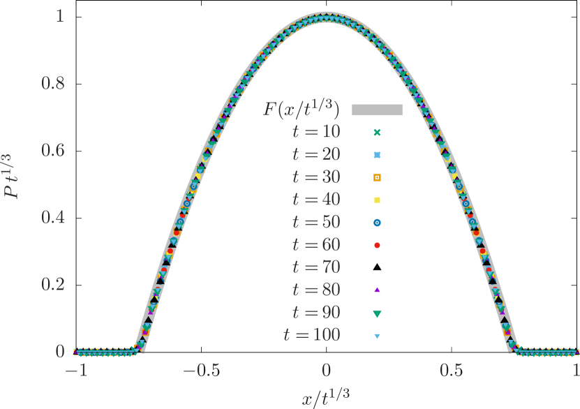
Figure 3: Rescaled solutions of the porous medium equation, Eq. (13) with a Dirac delta function as the initial condition, showing the collapse predicted in Eq. (14).

Note that this theoretical framework suggests that the spread of the particle cloud will grow sub-diffusively, $\sigma\sim t^{1/3}$.

It is relevant to ask ourselves about the validity regime of the previous approximation. For example, we have considered the limit $t_{0}\to 0$ in the determination of Eq. (10). This approximation is valid when $t_{0}$ is small compared to the time scale required for particles to jump over a ${\cal J}_{0}$ link, i.e. ${\cal J}_{0}^{-1}$, which will be the case for all our simulations. Moreover, we assume that the probability distribution and the hopping rates are smooth enough, which need not be the case for a single sample, but will be true for the ensemble average.

IV Numerical Simulations

We have considered an $L=200$ chain with periodic boundaries, using ${\cal J}_{1}=1$, $t_{0}=10$ and $\Delta t=1$, similarly to the two histories shown in Fig. 2 (a). In our simulations $N_{P}=25$, $50$, 100 or 200 particles, and ${\cal J}_{0}=10^{-6}$, $10^{-4}$ or $10^{-2}$. In all cases, we have simulated up to time $T_{\text{max}}=10^{8}$, taking $N_{S}=2000$ samples (unless otherwise stated). Throughout this section we define $x_{p,s}(t)$ as the position of particle $p$ in sample $s$ at time $t$, and $J_{i,s}(t)$ as the hopping probability between sites $i$ and $i+1$ in sample $s$ at time $t$. The initial condition is given by

$$x_{p,s}(0)=L/2,\qquad p s$$ for all and , (15)

$$J_{i,s}(0)={\cal J}_{0},\qquad i s$$ for all and . (16)

We must make a distinction between averaging over all particles within each sample, $E_{P}[\cdot]$, averaging over all samples, $E_{S}[\cdot]$, and averaging over both simultaneously, $E_{SP}[\cdot]$, defined as

$$E_{S}[q_{s}] \equiv{1\over N_{S}}\sum_{s=1}^{N_{S}}q_{s},$$ (17)

$$E_{P}[q_{p}] \equiv{1\over N_{P}}\sum_{p=1}^{N_{P}}q_{p},$$ (18)

$$E_{SP}[q_{p,s}] \equiv E_{S}[E_{P}[q_{p,s}]]=E_{P}[E_{S}[q_{p,s}]],$$ (19)

where $q_{s}$, $q_{p}$ and $q_{p,s}$ are observables associated to each sample, each particle or both. Also, we can define the corresponding variances, $\sigma_{\cal O}^{2}[X]\equiv E_{\cal O}[X^{2}]-E_{\cal O}[X]^{2}$, for ${\cal O}\in\{S,P,SP\}$.

We have considered the evolution of the average width of the particle cloud, defined in two alternative ways. First of all, we can consider the global deviation of the positions of all particles in all samples,

$$W_{\text{all}}(t)=\sigma_{SP}[x_{p,s}(t)],$$ (20)

and we can compare it with the average value of the widths of each sample, which is defined as

$$W^{2}_{\text{av}}(t)=E_{S}[\sigma^{2}_{P}[x_{p,s}(t)]].$$ (21)

Necessarily, the deviation of the whole ensemble of particle positions must exceed (or be equal to) the average of the deviations within each sample,

$$W_{\text{all}}(t)\geq W_{\text{av}}(t).$$ (22)

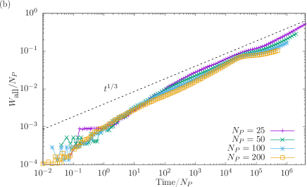
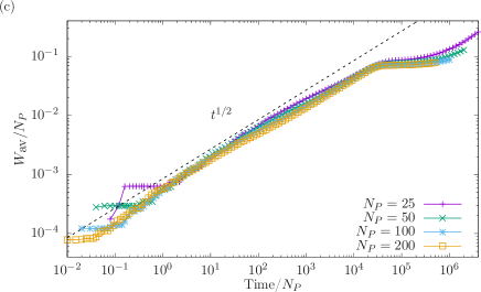
Figure 4: Average width of the particle cloud, as a function of time. (a) Comparison of $W_{\text{all}}(t)$, Eq. (20), and $W_{\text{av}}(t)$, Eq. (21), using $N_{P}=200$ and three different values for ${\cal J}_{0}=10^{-6}$, $10^{-4}$ and $10^{-2}$. The top straight line shows a $t^{1/2}$ behavior, and the lower one $t^{1/3}$. Notice that inequality (22) holds exactly in all cases. (b) $W_{\text{all}}$ as a function of time for ${\cal J}_{0}=10^{-6}$, both rescaled with the number of particles $N_{P}$, showing the power-law $t^{1/3}$. (c) $W_{\text{av}}$ as a function of time for ${\cal J}_{0}=10^{-6}$, rescaled in the same way, while the dashed line represents $t^{1/2}$.

Fig. 4 (a) shows both widths using $N_{P}=200$ and three different values of ${\cal J}_{0}$. Both widths grow approximately as a power-law for a broad range of times. For ${\cal J}_{0}=10^{-2}$ both widths coincide, growing diffusively (dashed-dotted line denotes $t^{1/2}$) up to a certain saturation time, while for ${\cal J}_{0}=10^{-4}$ we observe a significant difference between $W_{\text{all}}$ and $W_{\text{av}}$ only for short times (notice that the vertical axis is in logarithmic scale), and a wide time range in which both grow as $t^{1/3}$. For ${\cal J}_{0}=10^{-6}$, on the other hand, we see a more significant difference between both widths. After an initial transient time, $W_{\text{av}}$ grows diffusively up to times $\sim 10^{7}$ whereas the growth of $W_{\text{all}}$ is mostly subdiffusive, particularly in the interval $t\approx 5\cdot 10^{5}$ to $t\approx 10^{7}$. From that moment on, $W_{\text{av}}$ approximately saturates whereas $W_{\text{all}}$ keeps growing. The next sections will provide a physical picture for that complex behavior. Indeed, we contend that $W_{\text{all}}$ corresponds approximately to the expected behavior for the width of the particle cloud predicted in by the continuum approximation for very low ${\cal J}_{0}$, provided by the scaling of the PME, Eq. (13), as we can see in Eq. (14). The reasons for the gap between $W_{\text{all}}$ and $W_{\text{av}}$ will be discussed in the next section, and are related to the absence of self-averaging.

In Fig. 4 (b) and (c) we see that both $W_{\text{all}}$ (b) and $W_{\text{av}}$ (c) collapse approximately for ${\cal J}_{0}=10^{-6}$ when the time and width axes are rescaled dividing by the number of particles $N_{P}$.

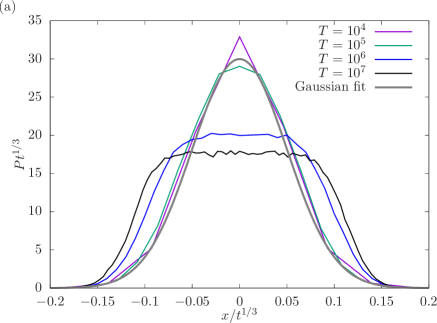
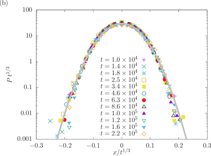
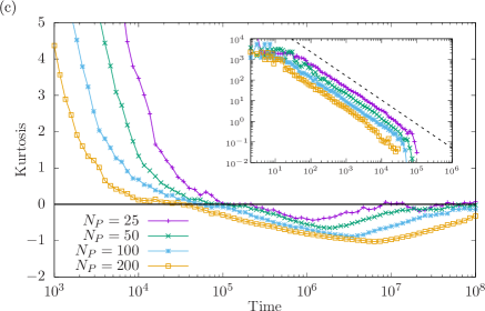
Figure 5: Rescaled particle histograms for different times using $N_{P}=200$ and ${\cal J}_{0}=10^{-6}$. (a) Histograms for the particle positions obtained for $N_{S}=2000$ samples, scaled using Eq. (14), as in Fig. 3. We can observe that short-term histograms collapse up to $t\sim 10^{5}$, when they start flattening. For even longer times, $t\sim 10^{8}$, the scaled histogram becomes closer to the initial collapse. (b) Scaled histogram data for 12 different times between $t=10^{4}$ and $t=2.2\cdot 10^{5}$, in logarithmic scale, showing that the collapse extends also to low probability values. The continuous line corresponds to a Gaussian distribution. (c) Time evolution of the (excess) kurtosis of the particle histograms for different values of $N_{P}$. Inset: log-log plot of the same data, showing a scaling law, Kurt $\sim t^{-7/6}$.

The full histogram for the particle positions, considering all $N_{S}=2000$ samples simultaneously, is provided in Fig. 5, for different times using $N_{P}=200$. The histograms are rescaled following Eq. (14), as in Fig. 3. For short times, the histograms collapse, increasing their width substantially between $t\sim 10^{5}$ and $10^{7}$. The accuracy of the collapse can be appreciated in Fig. 5 (b), where we can see the rescaled histograms for 20 times chosen between $t=10^{4}$ and $t=2\cdot 10^{5}$ in logarithmic scale. Remarkably, also the low probabilities seem to collapse around a Gaussian shape, as seen in the continuous line. Interestingly, the scaling function predicted by the PME is not a Gaussian but an inverted parabola (see Appendix A).

Further information about the histograms can be obtained by measuring the (excess) kurtosis, defined as

$$\text{Kurt}[x_{p,s}]={E_{SP}\left[\left(x_{p,s}-E_{SP}[x_{p,s}]\right)^{4}\right]\over\left(\sigma_{SP}[x_{p,s}]\right)^{4}}-3,$$ (23)

which is shown in Fig. 5 (c). We can observe that, for short times, the distributions are extremely leptokurtic (peaked), with the kurtosis decreasing approximately as $\kappa\sim t^{-7/6}$ for short times. Afterwards, it becomes negative (platykurtic, square-like) and evolves slowly towards zero, i.e. Gaussian-like.

IV.1 Active hoppings

The size of the cloud can be accessed also through an analysis of the set of hopping probabilities, $\{J_{i}\}_{i=1}^{L}$. Let us consider the observable

$$N_{J}={1\over{\cal J}_{1}-{\cal J}_{0}}\sum_{i=1}^{L}(J_{i}-{\cal J}_{0}).$$ (24)

If all $J_{i}$ are either ${\cal J}_{0}$ or ${\cal J}_{1}$, $N_{J}$ measures the number of ${\cal J}_{1}$ values. Fig. 6 (a) represents the expected value, $E_{S}[N_{J}]$, scaled with the number of particles $N_{P}$, as a function of time, also divided by $N_{P}$. We observe a similar behavior to $W_{\text{av}}(t)$, with a time range presenting $t^{1/2}$ scaling followed by saturation. We may also ask about the fluctuations in the size of the particle cloud, by measuring $\sigma_{S}[N_{J}]$, which appears in Fig. 6 (b). In this case, the curves for different $N_{P}$ do not collapse unless we scale differently the time axis (dividing by $N_{P}$) and $\sigma_{S}[N_{J}]$, which should be divided by $N_{P}^{1/2}$, as we show in the inset, in logarithmic scale. We observe a steady increase of $\sigma_{S}[N_{J}]$ with time, presenting two different scaling regimes: an initial $t^{1/2}$ followed by a $t^{1/4}$ regime, before reaching a quick decay at the saturation time towards a constant value. This behavior points at a possible dynamical phase transition at the saturation point. The physical reason for this behavior will be clarified in the next section, after several other observables have been considered.

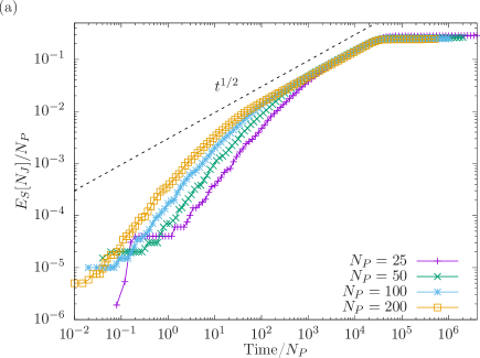
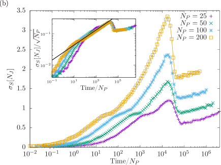
Figure 6: (a) Average number of active hopping probabilities as a function of time using ${\cal J}_{0}=10^{-6}$, both scaled with the number of particles $N_{P}$, compare to Fig. 4 (c). The continuous line corresponds to a $t^{1/2}$ scaling. (b) Sample-to-sample deviation of that magnitude. Inset: scaling with the square root of the number of particles makes the curves collapse around the peak. The continuous line represents a scaling of $t^{1/4}$.

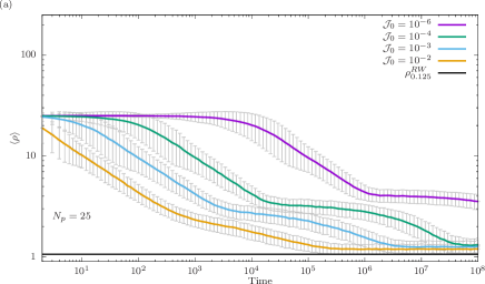
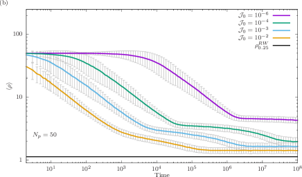
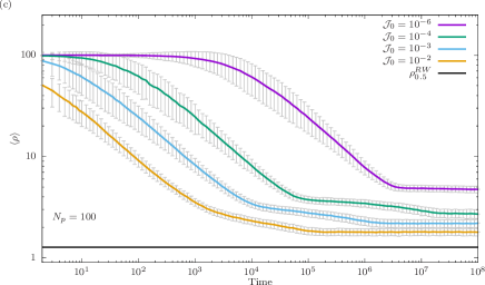
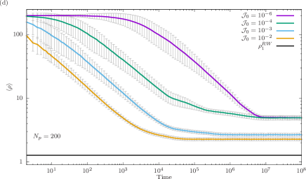
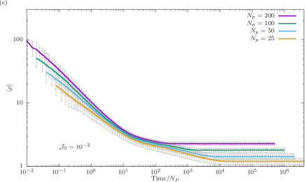
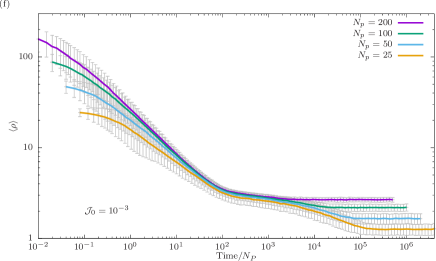
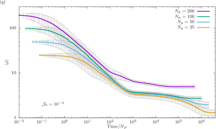
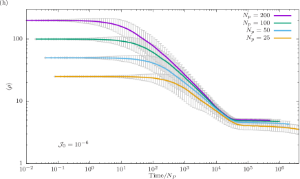
Figure 7: Average population-weighted density, $\left<\rho\right>$, as defined by Eq. (25), for (a) $N_{P}=25$, (b) $N_{P}=50$, (c) $N_{P}=100$ and (d) $N_{P}=200$ particles with different values of ${\cal J}_{0}$, and for (e) ${\cal J}_{0}=10^{-2}$, (f) ${\cal J}_{0}=10^{-3}$, (g) ${\cal J}_{0}=10^{-4}$ and (h) ${\cal J}_{0}=10^{-6}$ with different values of $N_{P}$. In the last four panels, time is divided by $N_{P}$. The minimum number of samples is $N_{S}=500$. Notice that the initial value is always $\left<\rho(0)\right>=N_{P}$. The horizontal bars in panels (a-d) correspond to the theoretical prediction for independent random walkers, Eq. (26).

IV.2 Population-averaged density

A relevant measure of particle correlations can be borrowed from demographics, where an interesting distinction is made between the average population density and the experienced density, also called population-weighted density, defined as the average local density experienced by a randomly selected individual Ottensmann.18 . For a lattice system, it can be defined from the local occupations $n_{i}$, i.e. the number of particles at site $i$,

$$\left<\rho\right>={1\over N_{P}}\sum_{i=1}^{L}n_{i}^{2},$$ (25)

in other terms, it is related to the Rényi entropy of order 2. Notice that if the occupation is homogeneous, $n_{i}=N_{P}/L$ and $\left<\rho\right>=N_{P}/L$. Fig. 7 shows the expected value of the population-weighted density of this system for different numbers of particles: (a) $N_{P}=25$, (b) $N_{P}=50$, (c) $N_{P}=100$ and (d) $N_{P}=200$, using four values of ${\cal J}_{0}=10^{-6}$, $10^{-4}$, $10^{-3}$ and $10^{-2}$. The horizontal bar in all cases corresponds to the theoretical prediction for independent random walkers for a density $\lambda\equiv N_{P}/L$,

$$\rho^{RW}_{\lambda}={\lambda\over 1-\exp(-\lambda)},$$ (26)

as it is proved in Appendix B. For very short times, $\left<\rho\right>=N_{P}$, because all particles are together at the origin. The values of $\left<\rho(t)\right>$ decay and seem to stabilize at a finite value $\rho_{\infty}$ in the $t\to\infty$ limit, which depends both on ${\cal J}_{0}$ and $N_{P}$. In all cases $\rho_{\infty}>\rho^{RW}_{\lambda}$, showing that the particles present strong interactions.

Panels (e-h) of Fig. 7 show the population-weighted density for (e) ${\cal J}_{0}=10^{-2}$, (f) ${\cal J}_{0}=10^{-3}$, (g) ${\cal J}_{0}=10^{-4}$ and (h) ${\cal J}_{0}=10^{-6}$ with the values of $N_{P}$ considered above, i.e. they show the same data as panels (a-d) organized differently. Moreover, time is divided by $N_{P}$ in all of them. We observe that $\rho_{\infty}$ grows steadily with $N_{P}$ for ${\cal J}_{0}=10^{-2}$, presents jumps with $N_{P}$ for ${\cal J}_{0}=10^{-3}$ and ${\cal J}_{0}=10^{-4}$, and sticks to a value $\rho_{\infty}\approx 5$ for all particle numbers when ${\cal J}_{0}=10^{-6}$. This value can be understood through inspection of Fig. 2 (a), where we see that the cloud occupies a region of size $L_{0}\approx 40$ sites. If the density is homogeneous in this region, the experienced density will be of order $N_{P}/L_{0}\approx 5$. This result is also compatible with the observed cloud size estimated through $W_{\text{av}}$ and $N_{J}$ which can be read from Fig. 4 and 6. Interestingly, for ${\cal J}_{0}=10^{-4}$ the system reaches the same final density, even though the width is much larger. The reason is that the cloud breaks down into clusters with the same final density, $\approx 5$. For ${\cal J}_{0}=10^{-2}$, on the other hand, the final density $\rho_{\infty}\approx 2.3$, still substantially above the value for independent random walkers, which is $\rho_{1}^{RW}\approx 1.582$ for this density $\lambda=N_{P}/L=1$ according to Eq. (26).

It is also interesting to observe the different stages shown in panels (e-h) of Fig. 7. We can distinguish a first initial stage, for which the cloud remains concentrated near a single point. This is followed by a decay stage, which corresponds to the expanding cloud and, for low ${\cal J}_{0}$, the PME phase. This stage ends in a plateau when the cloud is able to break down, at a time corresponding to the saturation of $W_{\text{av}}$ in Fig. 4 (c) and the peak of $\sigma_{S}[N_{J}]$ in Fig. 6 (b). The reader is also referred to Fig. 2, to check the typical configurations in all the cases. The plateau may still give rise to further discrete decays for intermediate values of ${\cal J}_{0}$, presumably when the island structure changes.

IV.3 Center of mass and correlations

The sub-diffusive expansion of the cloud signals an effective attraction between the particles, which is associated to strong correlations between their positions. We will characterize these correlations using the fluctuations of the center of mass (CM) as a proxy. Indeed, for every time and sample we can define

$$X_{CM,s}(t)\equiv E_{P}[x_{p,s}(t)],$$ (27)

and, along with it, the sample-to-sample fluctuations of this magnitude,

$$\sigma_{CM}(t)\equiv\sigma_{S}[E_{P}[x_{p,s}(t)]],$$ (28)

which are strongly tied to the difference between $W_{\text{all}}$ and $W_{\text{av}}$ expressed in inequality (22). Indeed,

$$W^{2}_{\text{all}}-W^{2}_{\text{av}}=E_{S}[E_{P}[x_{p,s}]^{2}]-E_{S}[E_{P}[x_{p,s}]]^{2}=\sigma^{2}_{CM},$$ (29)

i.e. they correspond to the distance between both curves in Fig. 4 (a), see inequality (22). Moreover, it can also be proved that

$$\sigma^{2}_{CM} ={1\over N_{P}^{2}}\sum_{p,q=1}^{N_{P}}\left(E_{S}[x_{p,s}x_{q,s}]-E_{S}[x_{p,s}]E_{S}[x_{q,s}]\right)$$

$$\equiv{1\over N_{P}^{2}}\sum_{p,q}C_{p,q},$$ (30)

where we have defined $C_{p,q}$ as the average over samples of the correlation between particles $p$ and $q$, and we have dropped the dependence on $t$ for convenience. Given the symmetry between particles, we must have $C_{p,q}=C_{0}\delta_{p,q}+C_{1}(1-\delta_{p,q})$. For uncorrelated random walkers $C_{1}=0$ and $C_{0}=Dt$, so we have

$$\sigma^{2}_{CM}={Dt\over N_{P}},$$ (31)

as expected. Yet, if each particle moves diffusively but correlations are as strong as possible, $C_{1}=C_{0}=Dt$, we have

$$\sigma^{2}_{CM}=Dt.$$ (32)

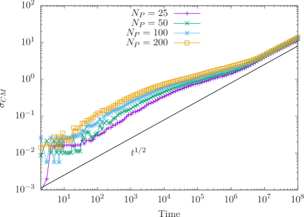
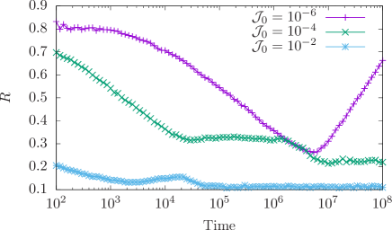
Figure 8: (a) Fluctuations of the center of mass of the particle cloud, for different numbers of particles using ${\cal J}_{0}=10^{-6}$. The straight line represent a $t^{1/2}$ growth. (b) Correlation ratio, $R$, defined in Eq. (33), as a function of time (in log scale), using $N_{P}=200$ and different values of ${\cal J}_{0}=10^{-6}$, $10^{-4}$ and $10^{-2}$.

The actual behavior of $\sigma_{CM}(t)$ is shown in Fig. 8 (a) for different numbers of particles as a function of time. We observe an intermediate regime where the fluctuations of the center of mass grow slowly, followed by a long-term diffusive scaling with $t^{1/2}$. But the most relevant observation is that, in this regime, the fluctuations of the center of mass do not depend on the number of particles, thus showing a behavior similar to Eq. (32). Each particle follows a random walk, but all particles are strongly correlated and the center of mass provides evidence for this.

Indeed, we can define a correlation ratio,

$$R\equiv{\sigma_{CM}\over W_{\text{all}}}\in[0,1],$$ (33)

which is zero for a large number of uncorrelated particles, and tends to one for strongly correlated walkers. Fig. 8 (b) shows the value of this ratio as a function of time for $N_{P}=200$ and different values of ${\cal J}_{0}=10^{-6}$, $10^{-4}$ and $10^{-2}$. Indeed, we observe that the correlation ratio is very low for large values of ${\cal J}_{0}$, which corresponds to independent random walkers. Yet, for very low ${\cal J}_{0}\approx 10^{-6}$ its behavior is more intriguing. It starts at a high value, decreasing logarithmically as the particle cloud expands until it reaches a minimum value, and starts a new logarithmic growth stage when the cloud has reached maximal expansion.

V Physical picture

The numerical data described in the previous section allow us to provide a physical picture for the statistical properties of the cloud of random walkers and the metric field in the RWDM model, based on the strong correlations between the positions of the particles, signalled by several observables, such as the difference between $W_{\text{all}}$ and $W_{\text{av}}$, the long term behavior of the population-averaged density $\left<\rho\right>$ or the correlation ratio $R$.

Evolution starts with all the particles concentrated at the center waiting to hop on a ${\cal J}_{0}$ link, which will take a time $\sim(N_{P}{\cal J}_{0})^{-1}$. The first particle taking such a hop will make other particles follow, and the particle cloud as a whole will start hopping between two neighboring sites for a while, until a second particle hops on a new ${\cal J}_{0}$ link again, thus spreading the cloud. Notice that different samples will make different choices during these initial steps. Thus, the average width of each cloud becomes much smaller than the global width of the ensemble of all clouds. Yet, both magnitudes grow at different rates: each cloud grows diffusively, with $t^{1/2}$, see Fig. 4, while the global cloud grows subdiffusively, approximately with $t^{1/3}$, which corresponds to the global behavior of the solution of the PME, see Eq. (13) and (14). Thus, we find a reasonable fit between our theoretical and numerical models for a certain time range. Yet, we ought not to forget that our model is described by a highly non-linear partial differential equation, and therefore its validity is arguably limited to certain time regions.

As the cloud expands, internal links are close to their maximum possible value, ${\cal J}_{1}$. Thus, our estimate of the number of active links, $N_{J}$, defined as in (24) and shown in Fig. 6, presents the same power-law scaling as the average width of the clouds, $W_{\text{av}}$, as shown in the central panel of Fig. 4. Yet, the clouds can not expand without limit, because the average width grows faster than the global width. Moreover, the local density will decay, as shown in Fig. 7, and when it reaches a minimal value $\rho_{\infty}$, the cloud will either stop its expansion or break up into islands. The maximum size of the clouds is, therefore, an effect related to the finite number of particles, and scales linearly with $N_{P}$, as we can see in the saturation value of both $W_{\text{av}}$ and $N_{J}$. Notice that this saturation is not related to the finite size of the system. Furthermore, beyond this saturation there is a finite probability that some links will not be occupied for a time $>t_{0}$, thus allowing them to return to their low value, ${\cal J}_{0}$, as we can check in Fig. 2 (a-b), where we can observe how it separates into two or more islands. Of course, the continuum approximation provided by the PME is not valid beyond the saturation point.

At this point we observe a signature of a dynamical phase transition in the sudden fall of the deviation of the number of active hoppings, $\sigma_{S}[N_{J}]$, shown in Fig. 6 (b). We conjecture that this fall can be explained as follows. The clouds grow unbroken before saturation, with an increasing sample-to-sample variance. As they reach their asymptotical density they stop growing and they may break up into smaller fragments which do not present a tendency to expand. Saturated clouds, whether broken or unbroken, present a nearly fixed size, thus explaining the drop in the variance of $N_{J}$. Yet, the fragments can still wander, and $W_{\text{av}}$ can still grow. Yet, when the cloud remains unbroken $W_{\text{av}}$ saturates too.

Moreover, the ensemble formed by all the clouds will continue its expansion. Indeed, the sample-to-sample fluctuations of the CM of the clouds grow diffusively, providing evidence for our claim. Yet, these fluctuations of the CM provide a proxy measurement for the particle correlations, through Eq. (30). For large times and low ${\cal J}_{0}$, the fluctuations of the CM coincide for different numbers of particles, see Fig. 8 (a), providing evidence for strong internal correlations. Indeed, the correlation ratio $R$, defined in Eq. (33), takes much larger values for low ${\cal J}_{0}$, showing that a large fraction of the fluctuations of the cloud can be accounted for by the fluctuations of the center of mass, while the cloud behaves internally as a rigid cluster.

In the long term we conjecture that the system will consist of one or several clusters which will wander through the system. If the system size is infinite, they will eventually drift away from each other. Otherwise, they will collide into each other with a certain frequency, giving rise to a steady state in which clusters split up and merge together. These final stages present some similarities with the long-term behavior of galaxies in an expanding or steady-state universe.

VI Conclusions and further work

We have considered a model of random walkers on a deformable medium (RWDM), in which random walkers interact with the medium on which they move. Indeed, the hopping probability associated to each link becomes a dynamical variable, which gets higher when it is actually used, or relaxes towards a lower equilibrium value otherwise. The reinforcement of actually used paths presents similarities with neural plasticity: neurons that fire together wire together, also known as Hebb’s rule hertz.90 . Adaptable networks appear in a variety of settings, where usage of a link tends to reinforce its strength and, thus, the probability of further usage Gross ; Sayama . Moreover, the RWDM can also serve as a toy model of stochastic gravity since the medium can be considered as a (1+1)D metric, following the principle that matter tells geometry how to curve and geometry tells matter how to move.

The RWDM can be considered as a part of the family of reinforced random walks, with several relevant differences. Indeed, reinforced random walks enhance the probability of re-visiting nodes or edges, either permanently or temporarily. The RWDM extends these ideas to allow the jumping probabilities to become a full-fledged dynamical object.

For the sake of concreteness, we have focused on the 1D case, starting with an initial condition in which all particles are concentrated at the center, and the medium starts relaxed, in the limit in which the excited hopping is much larger than the equilibrium one, and for fast relaxation. In that limit, a continuum description should be provided by the porous medium equation (PME), which presents scaling solutions in this regime: our cloud should expand subdiffusively with time, due to self-localization effects, and grows like $\sim t^{1/3}$.

Indeed, this subdiffusive growth is observed in numerical experiments, but only when we consider the global cloud consisting of all samples, i.e. an average over the whole configuration space. On the other hand, when we consider the average over samples of the width of each cloud, we typically observe a diffusive behavior, $t^{1/2}$. Yet, the global width must necessarily exceed the average width, and their difference is related to the fluctuations of the center of mass of each cloud, which can also be linked to the internal correlations within the cloud. Thus, we were able to identify a growth regime and a saturated regime (not related to the system size), where the number of active links reaches a final asymptotic value, even though the global width can still grow because the center of mass of the cloud can still wander.

Statistical mechanics of the RWDM seems to provide a wealth of behaviors which are worth exploring, such as the extension to several dimensions or the spread of different initial configurations, which can give rise to structure formation. Also, the internal dynamics of the metric field can be extended in several interesting ways, such as introducing a surface tension which would allow for the propagation of waves. It is interesting to remark that the porous medium equation ruling the spread of the RWDM cloud is causal, while the heat equation is not. This fact might bear relevance for the study of relativistic brownian motion, which is still an open problem kostadt.13 . Moreover, critical behavior on a gravity field has been extensively studied using Liouville theory, giving rise to the well-known Knizhnik-Polyakov-Zamolodchikov (KPZ) equation which evaluates how the critical exponents of a 2D conformal field theory (CFT) deform in presence of gravity kpz.88 ; ambjorn.96 . We intend to explore all these connections in the forthcoming future.

Appendix A Solution of the porous medium equation

A general solution for the porous medium equation (13) with arbitrary exponent and a concentrated initial condition can be found in Pattle.59 ; vazquez.91 . Here we will provide a simplified version for the benefit of the reader, giving rise to the exact form of $F(\eta)$, with $\eta\equiv xt^{-1/3}$, in Eq. (14).

Symmetry and scaling considerations lead to the following proposal,

$$P(x,t)=\begin{cases}\frac{t^{-1/3}}{\alpha}\left[1-\left(\frac{x}{\beta t^{1/3}}\right)^{2}\right],&\text{if }|x|\leq\beta t^{1/3}\\ 0,&\text{otherwise}.\end{cases}$$ (34)

which corresponds to

$$F(\eta)=\max(0,1-\eta^{2}).$$ (35)

Normalization as a probability distribution leads to the condition

$${\alpha\over\beta}={4\over 3}.$$ (36)

Plugging expression (34) into Eq. (13) we obtain

$$\alpha\beta^{2}=6{\cal J}_{1}.$$ (37)

Thus, the values of $\alpha$ and $\beta$ are completely determined.

Appendix B Population-averaged density for independent random walkers

In the case of random walkers, the expected value of the population-averaged density can be obtained exactly through the following argument. Let us consider $N_{P}$ particles on $L$ sites. The probability that any of the sites will be empty is given by

$$p_{E}=\left({L-1\over L}\right)^{N_{P}},$$ (38)

and thus the probability of a particle being occupied is just $p_{O}=1-p_{E}$. The expected number of occupied sites is thus $Lp_{O}$, and the population-averaged density corresponds to the expected density within that set of occupied sites, $\rho_{\infty}=N_{P}/(Lp_{O})$. When $N_{P}/L=\lambda$ we have

$$\rho(L)_{\infty}^{RW}={\lambda\over 1-\left(1-{1\over L}\right)^{N_{p}}},$$ (39)

and in the thermodynamic limit we obtain

$$\rho_{\infty}^{RW}=\lim_{L\to\infty}{\lambda\over 1-\left(1-{1\over L}\right)^{N_{p}}}={\lambda\over 1-e^{-\lambda}}.$$ (40)

References

- (1) So-called because elephants are believed to have long term memory.
- (2) G.M. Schütz, S. Trimper, Elephants can always remember: exact long-range memory effects in a non-Markovian random walk, Phys. Rev. E 70, 045101(R) (2004).
- (3) N. Kumar, U. Harbola, K. Lindenberg, Memory-induced anomalous dynamics: Emergence of diffusion, subdiffusion, and superdiffusion from a single random walk model, Phys. Rev. E 82, 021101 (2010).
- (4) M.A.A. da Silva, G.M. Viswanathan, J.C. Cressoni, Ultraslow diffusion in an exactly solvable non-Markovian random walk, Phys. Rev. E 89, 052110 (2014).
- (5) M.J. Kearney, R.J. Martin, Random walks exhibiting anomalous diffusion: elephants, urns and the limits of normality, J. Stat. Mech. 013209 (2018).
- (6) D. Boyer, J.C.R. Romo-Cruz, Solvable random-walk model with memory and its relation with Markovian models of anomalous diffusion, Phys. Rev. E 90, 042136 (2014).
- (7) D. Boyer, C. Solis-Salas, Random walks with preferential relocations to places visited in the past and their applications to biology, Phys. Rev. Lett. 112, 240601 (2014).
- (8) D. Boyer, I. Pineda, Slow Lévy Walks, Phys. Rev. E 93, 022103 (2016).
- (9) A. Falcón-Cortés, D. Boyer, L. Giuggioli, S.N. Majumdar, Localization transition induced by learning in random searches, Phys. Rev. Lett. 119, 140603 (2017).
- (10) D. Campos, V. Méndez, Phase transitions in optimal search times: how random walkers should combine resetting and flight scales, Phys. Rev. E 92, 062115 (2015).
- (11) P.-G. de Gennes, Scaling concepts in polymer physics, Cornell Univ. Press (1979).
- (12) D.J. Amit, G. Parisi, L. Peliti, Asymptotic behavior of the ”true” self-avoiding walk, Phys. Rev. B 27, 1635 (1983).
- (13) C. Domb, G.S. Joyce, Cluster expansion for a polymer chain, J. Phys. C: Solid State Phys. 5, 956 (1972).
- (14) H.E. Stanley, K. Kang, S. Redner, R.L. Blumberg, Novel superuniversal behavior of a random walk model, Phys. Rev. Lett. 51, 1223 (1983).
- (15) R. Permantle, A survey of random processes with reinforcement, Prob. Surveys 4, 1 (2007).
- (16) H.G. Othmer, A. Stevens, Aggregation, blowup and collapse: the ABC’s of taxis in reinforced random walks, SIAM J. Appl. Math. 57, 1044 (1997).
- (17) B. Davis, Reinforced random walk, Probab. Theor. Rel. Fields 84, 203 (1990).
- (18) A. Ordemann, E. Tomer, G. Berkolaiko, S. Havlin, A. Bunde, Structural properties of self-attracting walks, Phys. Rev. E, 64, 046117 (2001).
- (19) J.G. Foster, P. Grassberger, M. Paczuski, Reinforced walks in two and three dimensions, New J. Phys. 11, 023009 (2009).
- (20) V.B. Sapozhnikov, Self-attracting walk with , J. Phys. A: Math. Gen. 27, L151 (1994).
- (21) S.Y. Huang, X.W. Zou, Z.Z. Jin, Multiparticle random walks on a deformable medium, Phys. Rev. E 66, 041112 (2002)
- (22) Z.J. Tan, X.W. Zou, S.Y. Huang, W. Zhang, Z.Z. Jin, Patterns of particle distribution in multiparticle systems by random walks with memory enhancement and decay, Phys. Rev. E 66, 011101 (2002).
- (23) F. Schweitzer, An agent-based in framework biological of and active social matter systems p with applications, Eur. J. Phys. 40, 014003 (2019).
- (24) O. Angel, N. Crawford, G. Kozma, Localization for linearly edge reinforced random walks, Duke Math. J. 163, 889 (2014).
- (25) M. Dorigo, G. di Caro, Ant colony optimization: A new meta-heuristic, in Proc. of the 1999 Congress on Evolutionary Computation, CEC 1999, pp. 1470 (1999); M. Dorigo, T. Stützle, Ant Colony Optimization, The MIT Press (2004).
- (26) P. Rabanal, I. Rodríguez, F. Rubio, Using river formation dynamics to design heuristic algorithms, in International Conference on Unconventional Computation, page 163, Springer (2007); P. Rabanal, I. Rodríguez, F. Rubio, Applications of river formation dynamics, J. Comp. Science 22, 26 (2017).
- (27) T. Miyazawa, T. Izuyuma, Diffusion in one-dimensional inhomogeneous media, Phys. Rev. A 36, 5791 (1987).
- (28) J.F. Bouchaud, A. Georges, Anomalous diffusion in disordered media: statistical mechanics, models and physical applications, Phys. Rep. 195, 127 (1990).
- (29) Y. Li, O. Kahraman, C.A. Haselwandter, Distribution of randomly diffusing particles in inhomogeneous media, Phys. Rev. E 96, 032139 (2017).
- (30) B.L. Hu, E. Verdaguer, Stochastic Gravity: Theory and Applications, Living Rev. Relativity 7, (2004).
- (31) Juan Luis Vazquez, The Porous Medium equation, Clarendon Press Oxford (2007).
- (32) We would like to stress that there are more efficient numerical algorithms available for our problem, based on the evaluation of waiting times, such as J.J. Lukien, J.P.L. Segers, P.A.J. Hilbers, R.J. Gelten, A.P.J. Jansen, Efficient Monte Carlo methods for the simulation of catalytic surface reactions, Phys. Rev. E 58, 2598 (1998).
- (33) J.R. Ottensmann, On population-weighted density, available at SSRN https://ssrn.com/abstract=3119965 (2018).
- (34) R.E. Pattle, Diffusion from an instantaneous point source with a concentration-dependent coefficient, Quart. J. Mech. and App. Math 12, 4 (1959).
- (35) J. Hertz, A. Krogh, R.G. Palmer, Neural computations, Addison Wesley (1990).
- (36) T. Gross, H. Sayama, Adaptive networks, Springer (2009).
- (37) H. Sayama et al., Modeling complex systems with adaptive networks, Comp. & Math. App. 65, 1645 (2013).
- (38) P. Kostädt, M. Liu, Causality and stability of the relativistic diffusion equation, Phys. Rev. D 62, 023003 (2013).
- (39) V. Knizhnik, A. Polyakov, A. Zamolodchikov, Fractal structure of 2d quantum gravity, Mod. Phys. Lett. A 3, 819 (1988).
- (40) J. Ambjørn, K.N.Anagnostopoulos, U.Magnea, G. Thorleifsson, Geometrical interpretations of the Knizhnik-Polyakov-Zamolodchikov, Phys. Lett. B 388, 713 (1996).