Generating Hierarchical Explanations on Text Classification via Feature Interaction Detection

Abstract

Generating explanations for neural networks has become crucial for their applications in real-world with respect to reliability and trustworthiness. In natural language processing, existing methods usually provide important features which are words or phrases selected from an input text as an explanation, but ignore the interactions between them. It poses challenges for humans to interpret an explanation and connect it to model prediction. In this work, we build hierarchical explanations by detecting feature interactions. Such explanations visualize how words and phrases are combined at different levels of the hierarchy, which can help users understand the decision-making of black-box models. The proposed method is evaluated with three neural text classifiers (LSTM, CNN, and BERT) on two benchmark datasets, via both automatic and human evaluations. Experiments show the effectiveness of the proposed method in providing explanations that are both faithful to models and interpretable to humans.

1 Introduction

Deep neural networks have achieved remarkable performance in natural language processing (NLP) (Devlin et al., 2018; Howard and Ruder, 2018; Peters et al., 2018), but the lack of understanding on their decision making leads them to be characterized as blackbox models and increases the risk of applying them in real-world applications (Lipton, 2016; Burns et al., 2018; Jumelet and Hupkes, 2018; Jacovi et al., 2018).

Understanding model prediction behaviors has been a critical factor in whether people will trust and use these blackbox models (Ribeiro et al., 2016). A typical work on understanding decision-making is to generate prediction explanations for each input example, called local explanation generation. In NLP, most of existing work on local explanation generation focuses on producing word-level or phrase-level explanations by quantifying contributions of individual words or phrases to a model prediction (Ribeiro et al., 2016; Lundberg and Lee, 2017; Lei et al., 2016; Plumb et al., 2018).

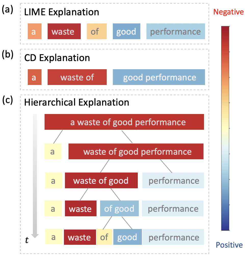
Figure 1: Different explanations for a negative movie review a waste of good performance, where the color of each block represents the contribution of the corresponding word/phrase/clause (feature) to the model prediction. From the hierarchical explanation, we obtain a set of features in each timestep ($t$), where the most important one is waste of good.

Figure 1 (a) and (b) present a word-level and a phrase-level explanation generated by the LIME (Ribeiro et al., 2016) and the Contextual Decomposition (CD) (Murdoch et al., 2018) respectively for explaining sentiment classification. Both explanations provide scores to quantify how a word or a phrase contributes to the final prediction. For example, the explanation generated by LIME captures a keyword waste and the explanation from CD identifies an important phrase waste of. However, neither of them is able to explain the model decision-making in terms of how words and phrases are interacted with each other and composed together for the final prediction. In this example, since the final prediction is negative, one question that we could ask is that how the word good or a phrase related to the word good contributes to the model prediction. An explanation being able to answer this question will give users a better understanding on the model decision-making and also more confidence to trust the prediction.

The goal of this work is to reveal prediction behaviors of a text classifier by detecting feature (e.g., words or phrases) interactions with respect to model predictions. For a given text, we propose a model-agnostic approach, called Hedge (for Hierarchical Explanation via Divisive Generation), to build hierarchical explanations by recursively detecting the weakest interactions and then dividing large text spans into smaller ones based on the interactions. As shown in Figure 1 (c), the hierarchical structure produced by Hedge provides a comprehensive picture of how different granularity of features interacting with each other within the model. For example, it shows how the word good is dominated by others in the model prediction, which eventually leads to the correct prediction. Furthermore, the scores of text spans across the whole hierarchy also help identify the most important feature waste of good, which can be served as a phrase-level explanation for the model prediction.

The contribution of this work is three-fold: (1) we design a top-down model-agnostic method of constructing hierarchical explanations via feature interaction detection; (2) we propose a simple and effective scoring function to quantify feature contributions with respect to model predictions; and (3) we compare the proposed algorithm with several competitive methods on explanation generation via both automatic and human evaluations. The experiments were conducted on sentiment classification tasks with three neural network models, LSTM Hochreiter and Schmidhuber (1997), CNN Kim (2014), and BERT Devlin et al. (2018), on the SST (Socher et al., 2013) and IMDB (Maas et al., 2011) datasets. The comparison with other competitive methods illustrates that Hedge provides more faithful and human-understandable explanations.

Our implementation is available at https://github.com/UVa-NLP/HEDGE.

2 Related Work

Over the past years, many approaches have been explored to interpret neural networks, such as contextual decomposition (CD) for LSTM (Murdoch et al., 2018) or CNN model (Godin et al., 2018), gradient-based interpretation methods (Hechtlinger, 2016; Sundararajan et al., 2017), and attention-based methods (Ghaeini et al., 2018; Lee et al., 2017; Serrano and Smith, 2019). However, these methods have limited capacity in real-world applications, as they require deep understanding of neural network architectures (Murdoch et al., 2018) or only work with specific models (Alvarez-Melis and Jaakkola, 2018). On the other hand, model-agnostic methods (Ribeiro et al., 2016; Lundberg and Lee, 2017) generate explanations solely based on model predictions and are applicable for any black-box models. In this work, we mainly focus on model-agnostic explanations.

2.1 Model-Agnostic Explanations

The core of generating model-agnostic explanations is how to efficiently evaluate the importance of features with respect to the prediction. So far, most of existing work on model-agnostic explanations focus on the word level. For example, Li et al. (2016) proposed Leave-one-out to probe the black-box model by observing the probability change on the predicted class when erasing a certain word. LIME proposed by Ribeiro et al. (2016) estimates individual word contribution locally by linear approximation from perturbed examples. A line of relevant works to ours is Shapley-based methods, where the variants of Shapley values (Shapley, 1953) are used to evaluate feature importance, such as SampleShapley (Kononenko et al., 2010), KernelSHAP (Lundberg and Lee, 2017), and L/C-Shapley (Chen et al., 2018). They are still in the category of generating word-level explanations, while mainly focus on addressing the challenge of computational complexity of Shapley values (Datta et al., 2016). In this work, inspired by an extension of Shapley values (Owen, 1972; Grabisch, 1997; Fujimoto et al., 2006), we design a function to detect feature interactions for building hierarchical model-agnostic explanations in subsection 3.1. While, different from prior work of using Shapley values for feature importance evaluation, we propose an effective and simpler way to evaluate feature importance as described in subsection 3.3, which outperforms Shapley-based methods in selecting important words as explanations in subsection 4.2.

2.2 Hierarchical Explanations

Addressing the limitation of word-level explanations (as discussed in section 1) has motivated the work on generating phrase-level or hierarchical explanations. For example, Tsang et al. (2018) generated hierarchical explanations by considering the interactions between any features with exhaustive search, which is computationally expensive.

Singh et al. (2019) proposed agglomerative contextual decomposition (ACD) which utilizes CD scores (Murdoch et al., 2018; Godin et al., 2018) for feature importance evaluation and employ a hierarchical clustering algorithm to aggregate features together for hierarchical explanation. Furthermore, Jin et al. (2019) indicated the limitations of CD and ACD in calculating phrase interactions in a formal context, and proposed two explanation algorithms by quantifying context independent importance of words and phrases.

A major component of the proposed method on feature interaction detection is based on the Shapley interaction index (Owen, 1972; Grabisch, 1997; Fujimoto et al., 2006), which is extended in this work to capture the interactions in a hierarchical structure. Lundberg et al. (2018) calculated features interactions via SHAP interaction values along a given tree structure. Chen and Jordan (2019) suggested to utilize a linguistic tree structure to capture the contributions beyond individual features for text classification. The difference with our work is that both methods (Lundberg et al., 2018; Chen and Jordan, 2019) require hierarchical structures given, while our method constructs structures solely based on feature interaction detection without resorting external structural information. In addition, different from Singh et al. (2019), our algorithm uses a top-down fashion to divide long texts into short phrases and words based on the weakest interactions, which is shown to be more effective and efficient in the experiments in section 4.

3 Method

This section explains the proposed algorithm on building hierarchical explanations (subsection 3.1) and two critical components of this algorithm: detecting feature interaction (subsection 3.2) and quantifying feature importance (subsection 3.3).

Algorithm 1 Hierarchical Explanation via Divisive Generation

1:  Input: text $\bm{x}$ with length $n$, and predicted label $\hat{y}$

2:  Initialize the original partition $\mathcal{P}_{0}\leftarrow\{\bm{x}_{(0,n]}\}$

3:  Initialize the contribution set $\mathcal{C}_{0}=\emptyset$

4:  Initialize the hierarchy $\mathcal{H}=[\mathcal{P}_{0}]$

5:  for $t=1,\dots,n-1$ do

6:     Find $\bm{x}_{(s_{i},s_{i+1}]}$ and $j$ by solving Equation 1

7:     Update the partition$\mathcal{P}_{t}^{\prime}\leftarrow\mathcal{P}_{t-1}\backslash\{\bm{x}_{(s_{i},s_{i+1}]}\}$$\mathcal{P}_{t}\leftarrow\mathcal{P}^{\prime}_{t}\cup\{\bm{x}_{(s_{i},j]},\bm{x}_{(j,s_{i+1}]}\}$

8:     $\mathcal{H}.add(\mathcal{P}_{t})$

9:     Update the contribution set $\mathcal{C}$ with$\mathcal{C}_{t}^{\prime}\leftarrow\mathcal{C}_{t-1}\cup\{(\bm{x}_{(s_{i},j]},\psi(\bm{x}_{(s_{i},j]}))\}$$\mathcal{C}_{t}\leftarrow\mathcal{C}_{t}^{\prime}\cup\{(\bm{x}_{(j,s_{i+1}]},\psi(\bm{x}_{(j,s_{i+1}]}))\}$

10:  end for

11:  Output: $\mathcal{C}_{n-1}$, $\mathcal{H}$

3.1 Generating Hierarchical Explanations

For a classification task, let $\bm{x}=(x_{1},\dots,x_{n})$ denote a text with $n$ words and $\hat{y}$ be the prediction label from a well-trained model. Furthermore, we define $\mathcal{P}=\{\bm{x}_{(0,s_{1}]},\bm{x}_{(s_{1},s_{2}]},\dots,\bm{x}_{(s_{P-1},n]}\}$ be a partition of the word sequence with $P$ text spans, where $\bm{x}_{(s_{i},s_{i+1}]}=(x_{s_{i}+1},\dots,x_{s_{i+1}})$. For a given text span $\bm{x}_{(s_{i},s_{i+1}]}$, the basic procedure of Hedge is to divide it into two smaller text spans $\bm{x}_{(s_{i},j]}$ and $\bm{x}_{(j,s_{i+1}]}$, where $j$ is the dividing point ($s_{i}<j<s_{i+1}$), and then evaluate their contributions to the model prediction $\hat{y}$.

Algorithm 1 describes the whole procedure of dividing $\bm{x}$ into different levels of text spans and evaluating the contribution of each of them. Starting from the whole text $\bm{x}$, the algorithm first divides $\bm{x}$ into two segments. In the next iteration, it will pick one of the two segments and further split it into even smaller spans. As shown in algorithm 1, to perform the top-down procedure, we need to answer the questions: for the next timestep, which text span the algorithm should pick to split and where is the dividing point?

Both questions can be addressed via the following optimization problem:

$$\min_{\bm{x}_{(s_{i},s_{i+1}]}\in\mathcal{P}}\min_{j\in(s_{i},s_{i+1})}\phi(\bm{x}_{(s_{i},j]},\bm{x}_{(j,s_{i+1}]}\mid\mathcal{P}),$$ (1)

where $\phi(\bm{x}_{(s_{i},j]},\bm{x}_{(j,s_{i+1}]}\mid\mathcal{P})$ defines the interaction score between $\bm{x}_{(s_{i},j]}$ and $\bm{x}_{(j,s_{i+1}]}$ given the current partition $\mathcal{P}$. The detail of this score function will be explained in subsection 3.2.

For a given $\bm{x}_{(s_{i},s_{i+1}]}\in\mathcal{P}$, the inner optimization problem will find the weakest interaction point to split the text span $\bm{x}_{(s_{i},s_{i+1}]}$ into two smaller ones. It answers the question about where the dividing point should be for a given text span. A trivial case of the inner optimization problem is on a text span with length 2, since there is only one possible way to divide it. The outer optimization answers the question about which text span should be picked. This optimization problem can be solved by simply enumerating all the elements in a partition $\mathcal{P}$. A special case of the outer optimization problem is at the first iteration $t=1$, where $\mathcal{P}_{0}=\{\bm{x}_{(0,n]}\}$ only has one element, which is the whole input text. Once the partition is updated, it is then added to the hierarchy $\mathcal{H}$.

The last step in each iteration is to evaluate the contributions of the new spans and update the contribution set $\mathcal{C}$ as in line 9 of the algorithm 1. For each, the algorithm evaluates its contribution to the model prediction with the feature importance function $\psi(\cdot)$ defined in Equation 5. The final output of algorithm 1 includes the contribution set $\mathcal{C}_{n-1}$ which contains all the produced text spans in each timestep together with their importance scores, and the hierarchy $\mathcal{H}$ which contains all the partitions of $\bm{x}$ along timesteps. A hierarchical explanation can be built based on $\mathcal{C}_{n-1}$ and $\mathcal{H}$ by visualizing the partitions with all text spans and their importance scores along timesteps, as Figure 1 (c) shows.

Note that with the feature interaction function $\phi(\cdot,\cdot)$, we could also design a bottom-up approach to merge two short text spans if they have the strongest interaction. Empirically, we found that this bottom-up approach performs worse than the algorithm 1, as shown in Appendix A.

3.2 Detecting Feature Interaction

For a given text span $\bm{x}_{(s_{i},s_{i+1}]}\in\mathcal{P}$ and the dividing point $j$, the new partition will be $\mathcal{N}=\mathcal{P}\backslash\{\bm{x}_{(s_{i},s_{i+1}]}\}\cup\{\bm{x}_{(s_{i},j]},\bm{x}_{(j,s_{i+1}]}\}=\{\bm{x}_{(0,s_{1}]},\dots,\bm{x}_{(s_{i},j]},\bm{x}_{(j,s_{i+1}]},\dots,\bm{x}_{(s_{P-1},n]}\}$. We consider the effects of other text spans in $\mathcal{N}$ when calculate the interaction between $\bm{x}_{(s_{i},j]}$ and $\bm{x}_{(j,s_{i+1}]}$, since the interaction between two words/phrases is closely dependent on the context (Hu et al., 2016; Chen et al., 2016). We adopt the Shapley interaction index from coalition game theory (Owen, 1972; Grabisch, 1997; Fujimoto et al., 2006) to calculate the interaction. For simplicity, we denote $\bm{x}_{(s_{i},j]}$ and $\bm{x}_{(j,s_{i+1}]}$ as $j_{1}$ and $j_{2}$ respectively. The interaction score is defined as (Lundberg et al., 2018),

$$\phi(j_{1},\!j_{2}\mid\!\mathcal{P})\!=\sum_{S\subseteq\mathcal{N}\backslash\{j_{1},j_{2}\}}\!\frac{|S|!(P-|S|-1)!}{P!}\gamma(j_{1},\!j_{2},\!S),$$ (2)

where $S$ represents a subset of text spans in $\mathcal{N}\backslash\{j_{1},j_{2}\}$, $|S|$ is the size of $S$, and $\gamma(j_{1},j_{2},S)$ is defined as follows,

$$\gamma(j_{1},\!j_{2},\!S) =\mathbb{E}[f(\bm{x}^{\prime})\!\mid\!S\cup\!\{j_{1},\!j_{2}\}]-\mathbb{E}[f(\bm{x}^{\prime})\!\mid\!S\cup\!\{j_{1}\}]$$ (3)

$$-\mathbb{E}[f(\bm{x}^{\prime})\mid S\cup\{j_{2}\}]+\mathbb{E}[f(\bm{x}^{\prime})\mid S],$$

where $\bm{x}^{\prime}$ is the same as $\bm{x}$ except some missing words that are not covered by the given subset (e.g. $S$), $f(\cdot)$ denotes the model output probability on the predicted label $\hat{y}$, and $\mathbb{E}[f(\bm{x}^{\prime})\mid S]$ is the expectation of $f(\bm{x}^{\prime})$ over all possible $\bm{x}^{\prime}$ given $S$. In practice, the missing words are usually replaced with a special token <pad>, and $f(\bm{x}^{\prime})$ is calculated to estimate $\mathbb{E}[f(\bm{x}^{\prime})|S]$ (Chen et al., 2018; Datta et al., 2016; Lundberg and Lee, 2017). We also adopt this method in our experiments. Another way to estimate the expectation is to replace the missing words with substitute words randomly drawn from the full dataset, and calculate the empirical mean of all the sampling data (Kononenko et al., 2010; Štrumbelj and Kononenko, 2014), which has a relatively high computational complexity.

With the number of text spans (features) increasing, the exponential number of model evaluations in Equation 2 becomes intractable. We calculate an approximation of the interaction score based on the assumption (Chen et al., 2018; Singh et al., 2019; Jin et al., 2019): a word or phrase usually has strong interactions with its neighbours in a sentence. The computational complexity can be reduced to polynomial by only considering $m$ neighbour text spans of $j_{1}$ and $j_{2}$ in $\mathcal{N}$. The interaction score is rewritten as

$$\phi(j_{1},\!j_{2}\!\mid\!\mathcal{P})\!=\!\sum_{S\subseteq\mathcal{N}_{m}\backslash\!\{j_{1},\!j_{2}\}}\!\frac{|S|!(M-|S|-2)!}{(M-1)!}\gamma(j_{1},\!j_{2},\!S),$$ (4)

where $\mathcal{N}_{m}$ is the set containing $j_{1}$, $j_{2}$ and their neighbours, and $M=|\mathcal{N}_{m}|$. In section 4, we set $m=2$, which performs well. The performance can be further improved by increasing $m$, but at the cost of increased computational complexity.

3.3 Quantifying Feature Importance

To measure the contribution of a feature $\bm{x}_{(s_{i},s_{i+1}]}$ to the model prediction, we define the importance score as

$$\begin{split}\psi(\bm{x}_{(s_{i},s_{i+1}]})=&f_{\hat{y}}(\bm{x}_{(s_{i},s_{i+1}]})\\ &-\max_{y^{\prime}\neq\hat{y},y^{\prime}\in\mathcal{Y}}f_{y^{\prime}}(\bm{x}_{(s_{i},s_{i+1}]}),\end{split}$$ (5)

where $f_{\hat{y}}(\bm{x}_{(s_{i},s_{i+1}]})$ is the model output on the predicted label $\hat{y}$; $\max_{y^{\prime}\neq\hat{y},y^{\prime}\in\mathcal{Y}}f_{y^{\prime}}(\bm{x}_{(s_{i},s_{i+1}]})$ is the highest model output among all classes excluding $\hat{y}$. This importance score measures how far the prediction on a given feature is to the prediction boundary, hence the confidence of classifying $\bm{x}_{(s_{i},s_{i+1}]}$ into the predicted label $\hat{y}$. Particularly in text classification, it can be interpreted as the contribution to a specific class $\hat{y}$. The effectiveness of Equation 5 as feature importance score is verified in subsection 4.2, where Hedge outperforms several competitive baseline methods (e.g. LIME (Ribeiro et al., 2016), SampleShapley (Kononenko et al., 2010)) in identifying important features.

4 Experiments

The proposed method is evaluated on text classification tasks with three typical neural network models, a long short-term memories (Hochreiter and Schmidhuber, 1997, LSTM), a convolutional neural network (Kim, 2014, CNN), and BERT (Devlin et al., 2018), on the SST (Socher et al., 2013) and IMDB (Maas et al., 2011) datasets, via both automatic and human evaluations.

4.1 Setup

Datasets.

We adopt the SST-2 (Socher et al., 2013) which has 6920/872/1821 examples in the train/dev/test sets with binary labels. The IMDB (Maas et al., 2011) also has binary labels with 25000/25000 examples in the train/test sets. We hold out 10% of the training examples as the development set.

Models.

The CNN model Kim (2014) includes a single convolutional layer with filter sizes ranging from 3 to 5. The LSTM Hochreiter and Schmidhuber (1997) has a single layer with 300 hidden states. Both models are initialized with 300-dimensional pretrained word embeddings Mikolov et al. (2013). We use the pretrained BERT model with 12 transformer layers, 12 self-attention heads, and the hidden size of 768, which was then fine-tuned with different downstream tasks to achieve the best performance. Table 1 shows the best performance of the models on both datasets in our experiments, where BERT outperforms CNN and LSTM with higher classification accuracy.

Models	Dataset
	SST	IMDB
LSTM	0.842	0.870
CNN	0.850	0.901
BERT	0.924	0.930

Table 1: The classification accuracy of different models on the SST and IMDB datasets.

Datasets	Methods	LSTM		CNN		BERT
		AOPC	Log-odds	AOPC	Log-odds	AOPC	Log-odds
SST	Leave-one-out	0.441	-0.443	0.434	-0.448	0.464	-0.723
	CD	0.384	-0.382	-	-	-	-
	LIME	0.444	-0.449	0.473	-0.542	0.134	-0.186
	L-Shapley	0.431	-0.436	0.425	-0.459	0.435	-0.809
	C-Shapley	0.423	-0.425	0.415	-0.446	0.410	-0.754
	KernelSHAP	0.360	-0.361	0.387	-0.423	0.411	-0.765
	SampleShapley	0.450	-0.454	0.487	-0.550	0.462	-0.836
	Hedge	0.458	-0.466	0.494	-0.567	0.479	-0.862
IMDB	Leave-one-out	0.630	-1.409	0.598	-0.806	0.335	-0.849
	CD	0.495	-1.190	-	-	-	-
	LIME	0.764	-1.810	0.691	-1.091	0.060	-0.133
	L-Shapley	0.637	-1.463	0.623	-0.950	0.347	-1.024
	C-Shapley	0.629	-1.427	0.613	-0.928	0.331	-0.973
	KernelSHAP	0.542	-1.261	0.464	-0.727	0.223	-0.917
	SampleShapley	0.757	-1.597	0.707	-1.108	0.355	-1.037
	Hedge	0.783	-1.873	0.719	-1.144	0.411	-1.126

Table 2: AOPCs and log-odds scores of different interpretation methods in explaining different models on the SST and IMDB datasets.

4.2 Quantitative Evaluation

We adopt two metrics from prior work on evaluating word-level explanations: the area over the perturbation curve (AOPC) (Nguyen, 2018; Samek et al., 2016) and the log-odds scores (Shrikumar et al., 2017; Chen et al., 2018), and define a new evaluation metric called cohesion-score to evaluate the interactions between words within a given text span. The first two metrics measure local fidelity by deleting or masking top-scored words and comparing the probability change on the predicted label. They are used to evaluate Equation 5 in quantifying feature contributions to the model prediction. The cohesion-score measures the synergy of words within a text span to the model prediction by shuffling the words to see the probability change on the predicted label.

AOPC.

By deleting top $k\%$ words, AOPC calculates the average change in the prediction probability on the predicted class over all test data as follows,

$$\text{AOPC}(k)=\frac{1}{N}\sum_{i=1}^{N}\{p(\hat{y}\mid\bm{x}_{i})-p(\hat{y}\mid\tilde{\bm{x}}^{(k)}_{i})\},$$ (6)

where $\hat{y}$ is the predicted label, $N$ is the number of examples, $p(\hat{y}\mid\cdot)$ is the probability on the predicted class, and $\tilde{\bm{x}}^{(k)}_{i}$ is constructed by dropping the $k\%$ top-scored words from $\bm{x}_{i}$. Higher AOPCs are better, which means that the deleted words are important for model prediction. To compare with other word-level explanation generation methods under this metric, we select word-level features from the bottom level of a hierarchical explanation and sort them in the order of their estimated importance to the prediction.

Log-odds.

Log-odds score is calculated by averaging the difference of negative logarithmic probabilities on the predicted class over all of the test data before and after masking the top $r\%$ features with zero paddings,

$$\text{Log-odds}(r)=\frac{1}{N}\sum_{i=1}^{N}\log\frac{p(\hat{y}\mid\tilde{\bm{x}}^{(r)}_{i})}{p(\hat{y}\mid\bm{x}_{i})}.$$ (7)

The notations are the same as in Equation 6 with the only difference that $\tilde{\bm{x}}^{(r)}_{i}$ is constructed by replacing the top $r\%$ word features with the special token $\langle\texttt{pad}\rangle$ in $\bm{x}_{i}$. Under this metric, lower log-odds scores are better.

Cohesion-score.

We propose cohesion-score to justify an important text span identified by Hedge. Given an important text span $\bm{x}_{(a,b]}$, we randomly pick a position in the word sequence $(x_{1},\ldots,x_{a},x_{b+1},\ldots,x_{n})$ and insert a word back. The process is repeated until a shuffled version of the original sentence $\bar{\bm{x}}$ is constructed. The cohesion-score is the difference between $p(\hat{y}\mid\bm{x})$ and $p(\hat{y}\mid\bar{\bm{x}})$. Intuitively, the words in an important text span have strong interactions. By perturbing such interactions, we expect to observe the output probability decreasing. To obtain a robust evaluation, for each sentence $\bm{x}_{i}$, we construct $Q$ different word sequences $\{\bar{\bm{x}}_{i}^{(q)}\}_{q=1}^{Q}$ and compute the average as

$$\text{Cohesion-score}=\frac{1}{N}\sum_{i=1}^{N}\frac{1}{Q}\sum_{q=1}^{Q}(p(\hat{y}\mid\bm{x}_{i})-p(\hat{y}\mid\bar{\bm{x}}_{i}^{(q)})),$$ (8)

where $\bar{\bm{x}}_{i}^{(q)}$ is the $q^{\text{th}}$ perturbed version of $\bm{x}_{i}$, $Q$ is set as 100, and the most important text span in the contribution set $\mathcal{C}$ is considered. Higher cohesion-scores are better.

4.2.1 Results

We compare Hedge with several competitive baselines, namely Leave-one-out (Li et al., 2016), LIME (Ribeiro et al., 2016), CD (Murdoch et al., 2018), Shapley-based methods, (Chen et al., 2018, L/C-Shapley), (Lundberg and Lee, 2017, KernelSHAP), and (Kononenko et al., 2010, SampleShapley), using AOPC and log-odds metrics; and use cohesion-score to compare Hedge with another hierarchical explanation generation method ACD (Singh et al., 2019).

Methods	Models	Cohesion-score
		SST	IMDB
Hedge	CNN	0.016	0.012
	BERT	0.124	0.103
	LSTM	0.020	0.050
ACD	LSTM	0.015	0.038

Table 3: Cohesion scores of Hedge and ACD in interpreting different models on the SST and IMDB datasets. For ACD, we adopt the existing application from the original paper (Singh et al., 2019) to explain LSTM on text classification.

The AOPCs and log-odds scores on different models and datasets are shown in Table 2, where $k=r=20$. Additional results of AOPCs and log-odds changing with different $k$ and $r$ are shown in Appendix B. For the IMDB dataset, we tested on a subset with 2000 randomly selected samples due to computation costs.

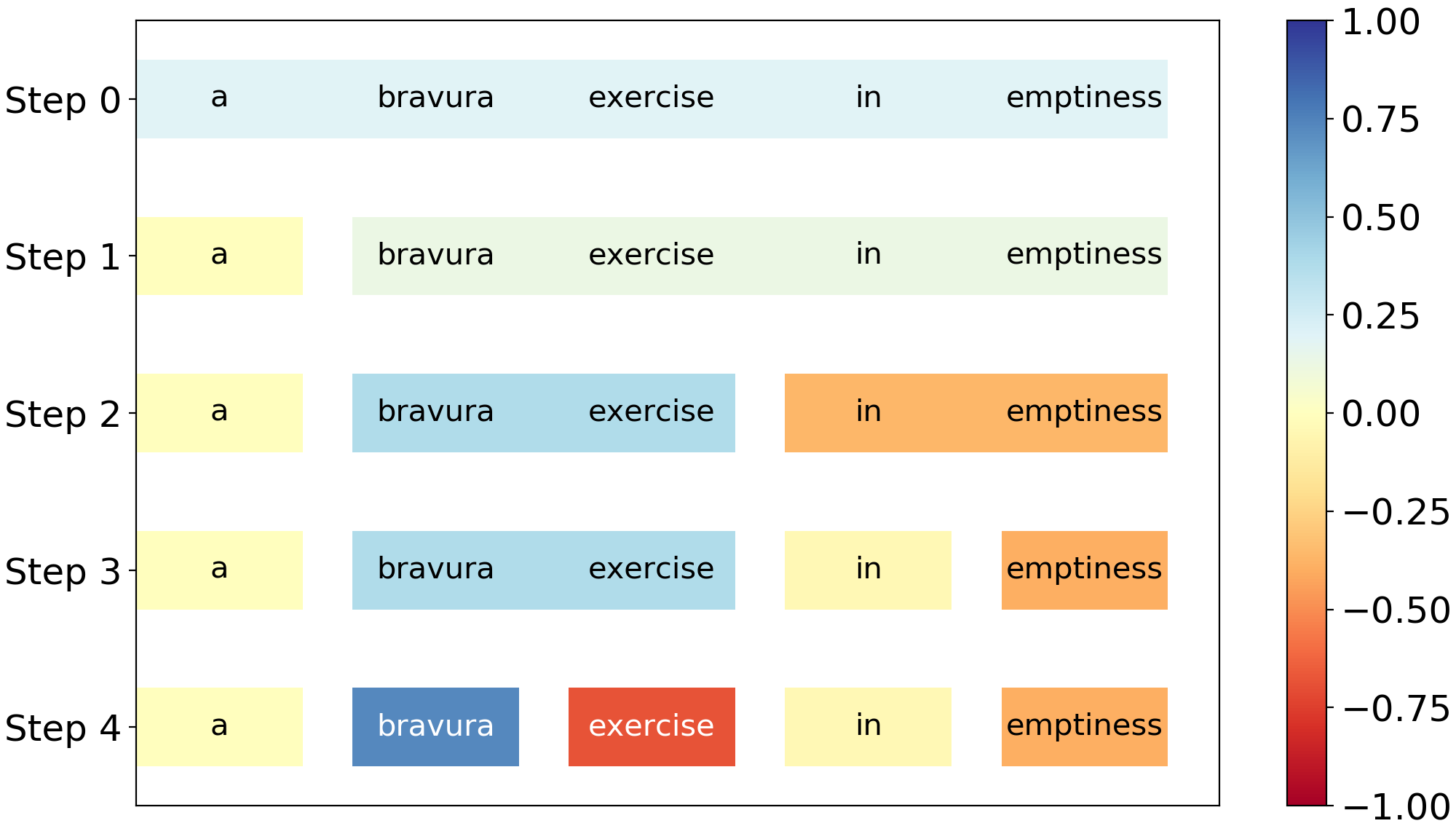
(a) Hedge for LSTM on the SST.

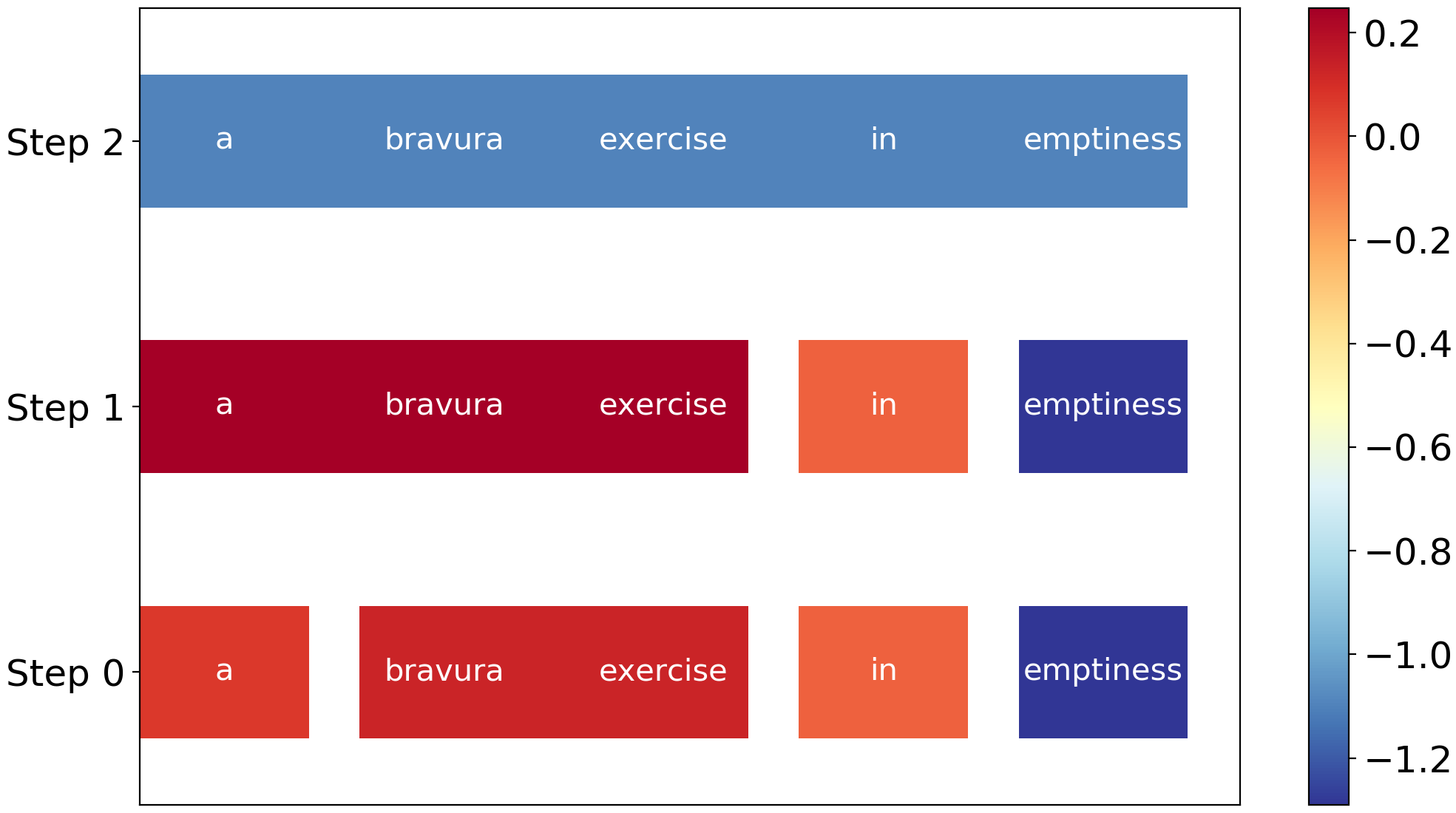
(b) ACD for LSTM on the SST.

Figure 2: Compare Hedge with ACD in interpreting the LSTM model on a negative movie review from the SST dataset, where LSTM makes a wrong prediction (positive). The importance scores of Hedge and CD scores are normalized for comparison.

Hedge achieves the best performance on both evaluation metrics. SampleShapley also achieves a good performance with the number of samples set as 100, but the computational complexity is 200 times than Hedge. Other variants, L/C-Shapley and KernelSHAP, applying approximations to Shapley values perform worse than SampleShapley and Hedge. LIME performs comparatively to SampleShapley on the LSTM and CNN models, but is not fully capable of interpreting the deep neural network BERT. The limitation of context decomposition mentioned by Jin et al. (2019) is validated by the worst performance of CD in identifying important words. We also observed an interesting phenomenon that the simplest baseline Leave-one-out can achieve relatively good performance, even better than Hedge when $k$ and $r$ are small. And we suspect that is because the criteria of Leave-one-out for picking single keywords matches the evaluation metrics. Overall, experimental results demonstrate the effectiveness of Equation 5 in measuring feature importance. And the computational complexity is only $\mathcal{O}(n)$, which is much smaller than other baselines (e.g. SampleShapley, and L/C-Shapley with polynomial complexity).

Table 3 shows the cohesion-scores of Hedge and ACD with different models on the SST and IMDB datasets. Hedge outperforms ACD with LSTM, achieving higher cohesion-scores on both datasets, which indicates that Hedge is good at capturing important phrases. Comparing the results of Hedge on different models, the cohesion-scores of BERT are significantly higher than LSTM and CNN. It indicates that BERT is more sensitive to perturbations on important phrases and tends to utilize context information for predictions.

4.3 Qualitative Analysis

For qualitative analysis, we present two typical examples. In the first example, we compare Hedge with ACD in interpreting the LSTM model. Figure 2 visualizes two hierarchical explanations, generated by Hedge and ACD respectively, on a negative movie review from the SST dataset. In this case, LSTM makes a wrong prediction (positive). Figure 2(a) shows Hedge correctly captures the sentiment polarities of bravura and emptiness, and the interaction between them as bravura exercise flips the polarity of in emptiness to positive. It explains why the model makes the wrong prediction. On the other hand, ACD incorrectly marks the two words with opposite polarities, and misses the feature interaction, as Figure 2(b) shows.

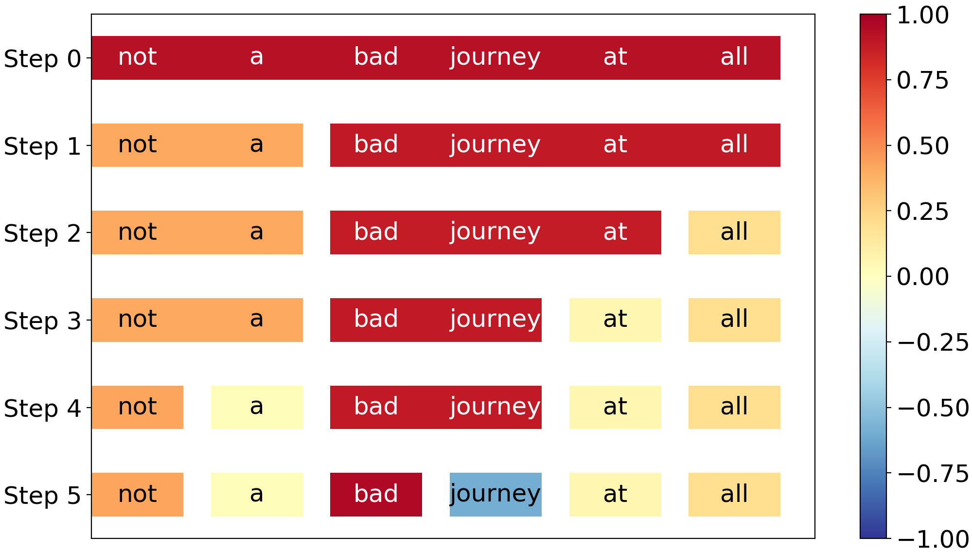
(a) Hedge for LSTM on SST.

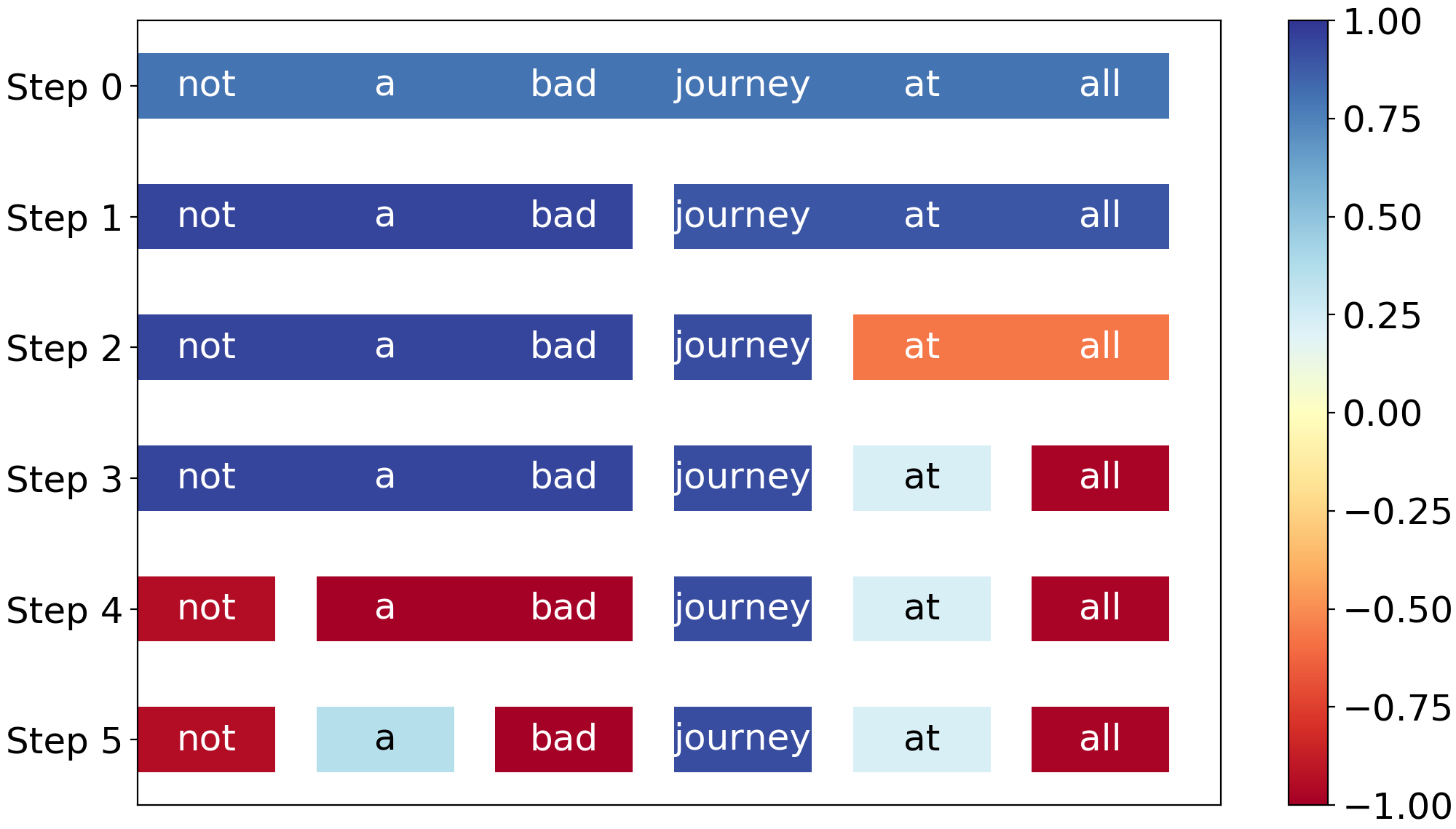
(b) Hedge for BERT on SST.

Figure 3: Compare Hedge in interpreting different models (LSTM and BERT) on a positive movie review from the SST dataset, where BERT makes the correct prediction (positive), while LSTM makes a wrong prediction (negative). Hedge explains that BERT captures the important phrase not a bad for making the correct prediction, while LSTM ignores it and is misled by the negative word bad.

In the second example, we compare Hedge in interpreting two different models (LSTM and BERT). Figure 3 visualizes the explanations on a positive movie review. In this case, BERT gives the correct prediction (positive), while LSTM makes a wrong prediction (negative). The comparison between Figure 3(a) and 3(b) shows the difference of feature interactions within the two models and explains how a correct/wrong prediction was made. Specifically, Figure 3(b) illustrates that BERT captures the key phrase not a bad at step 1, and thus makes the positive prediction, while LSTM (as shown in Figure 3(a)) misses the interaction between not and bad, and the negative word bad pushes the model making the negative prediction. Both cases show that Hedge is capable of explaining model prediction behaviors, which helps humans understand the decision-making. More examples are presented in Appendix C due to the page limitation.

4.4 Human Evaluation

We had 9 human annotators from the Amazon Mechanical Turk (AMT) for human evaluation. The features (e.g., words or phrases) with the highest importance score given by Hedge and other baselines are selected as the explanations. Note that Hedge and ACD can potentially give very long top features which are not user-friendly in human evaluation, so we additionally limit the maximum length of selected features to five. We provided the input text with different explanations in the user interface (as shown in Appendix D) and asked human annotators to guess the model’s prediction (Nguyen, 2018) from {“Negative”, “Positive”, “N/A”} based on each explanation, where “N/A” was selected when annotators cannot guess the model’s prediction. We randomly picked 100 movie reviews from the IMDB dataset for human evaluation.

There are two dimensions of human evaluation. We first compare Hedge with other baselines using the predictions made by the same LSTM model. Second, we compare the explanations generated by Hedge on three different models: LSTM, CNN, and BERT. We measure the number of human annotations that are coherent with the actual model predictions, and define the coherence score as the ratio between the coherent annotations and the total number of examples.

4.4.1 Results

Table 4 shows the coherence scores of eight different interpretation methods for LSTM on the IMDB dataset. Hedge outperforms other baselines with higher coherence score, which means that Hedge can capture important features which are highly consistent with human interpretations. LIME is still a strong baseline in providing interpretable explanations, while ACD and Shapley-based methods perform worse. Table 5 shows both the accuracy and coherence scores of different models. Hedge succeeds in interpreting black-box models with relatively high coherence scores. Moreover, although BERT can achieve higher prediction accuracy than the other two models, its coherence score is lower, manifesting a potential tradeoff between accuracy and interpretability of deep models.

Methods	Coherence Score
Leave-one-out	0.82
ACD	0.68
LIME	0.85
L-Shapley	0.75
C-Shapley	0.73
KernelSHAP	0.56
SampleShapley	0.78
Hedge	0.89

Table 4: Human evaluation of different interpretation methods with LSTM model on the IMDB dataset.

Models	Accuracy	Coherence scores
LSTM	0.87	0.89
CNN	0.90	0.84
BERT	0.97	0.75

Table 5: Human evaluation of Hedge with different models on the IMDB dataset.

5 Conclusion

In this paper, we proposed an effective method, Hedge, building model-agnostic hierarchical interpretations via detecting feature interactions. In this work, we mainly focus on sentiment classification task. We test Hedge with three different neural network models on two benchmark datasets, and compare it with several competitive baseline methods. The superiority of Hedge is approved by both automatic and human evaluations.

Appendix A Comparison between Top-down and Bottom-up Approaches

Given the sentence a waste of good performance for example, Figure 4 shows the hierarchical interpretations for the LSTM model using the bottom-up and top-down approaches respectively. Figure 4(a) shows that the interaction between waste and good can not be captured until the last (top) layer, while the important phrase waste of good can be extracted in the intermediate layer by top-down algorithm. We can see that waste flips the polarity of of good to negative, causing the model predicting negative as well. Top-down segmentation performs better than bottom-up in capturing feature interactions. The reason is that the bottom layer contains more features than the top layer, which incurs larger errors in calculating interaction scores. Even worse, the calculation error will propagate and accumulate during clustering.

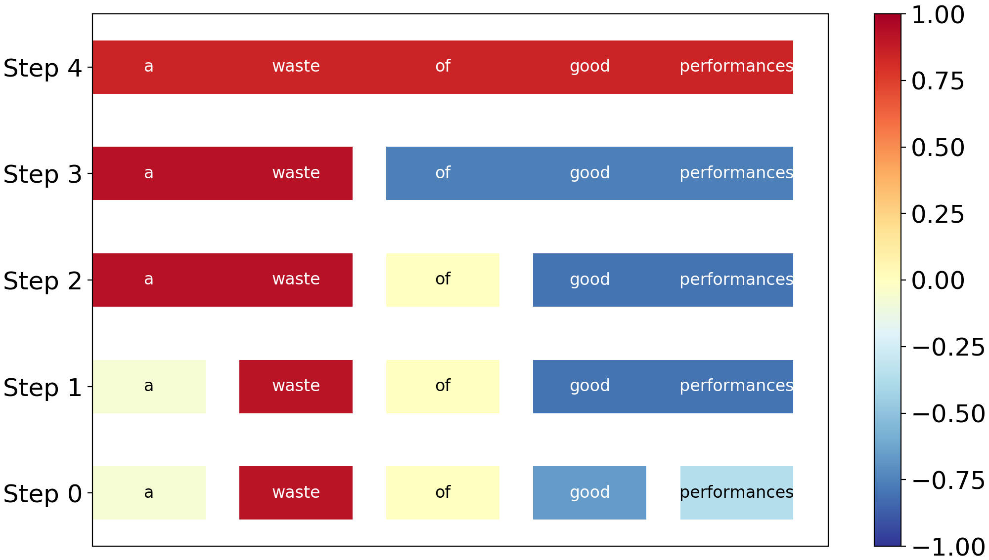
(a) Bottom-up clustering.

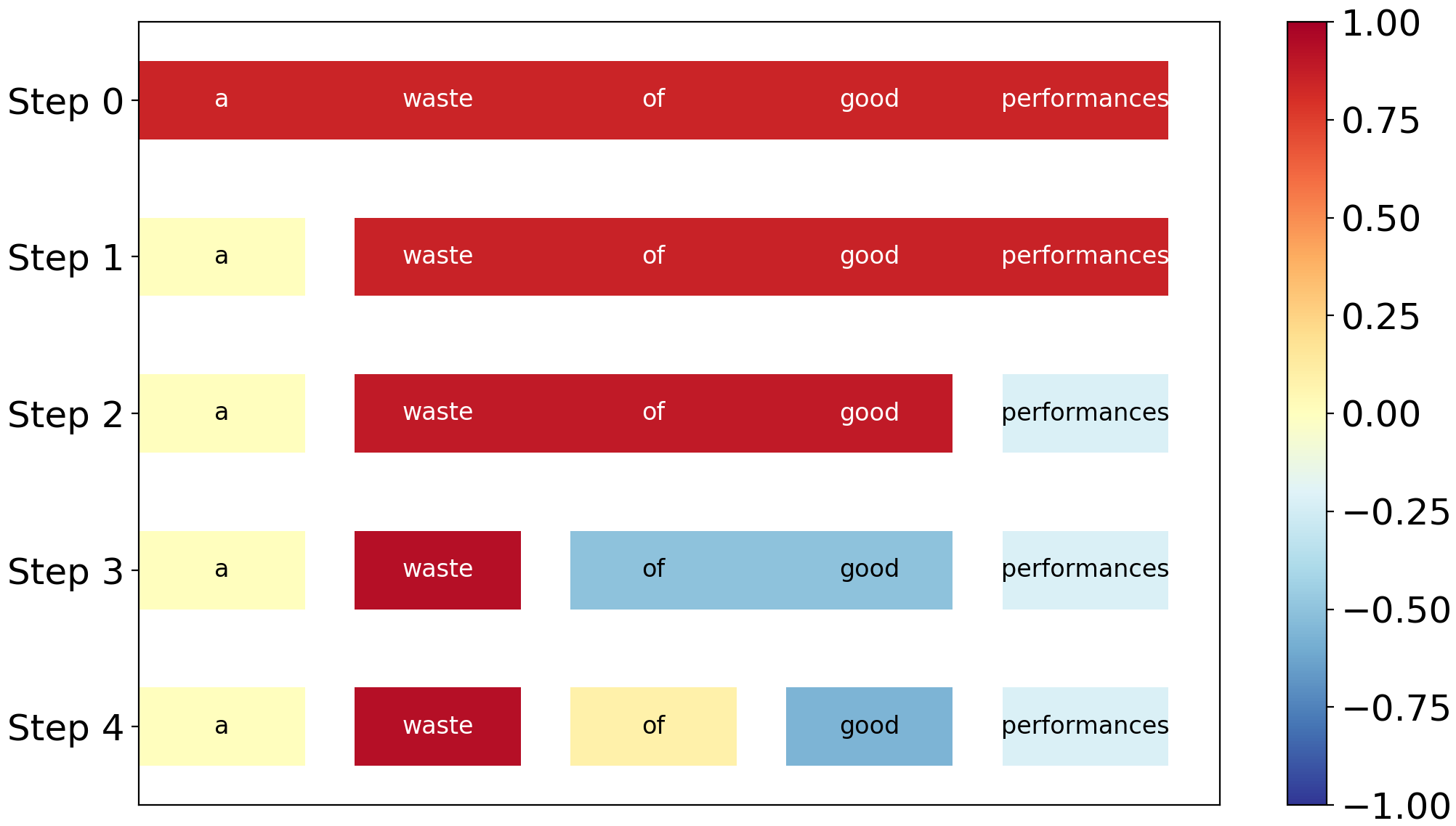
(b) Top-down segmentation.

Figure 4: Hierarchical interpretations for the LSTM model using the bottom-up and top-down approaches respectively. Red and green colors represent the negative and positive sentiments respectively.

Appendix B Results of AOPCs and log-odds changing with different $k$ and $r$

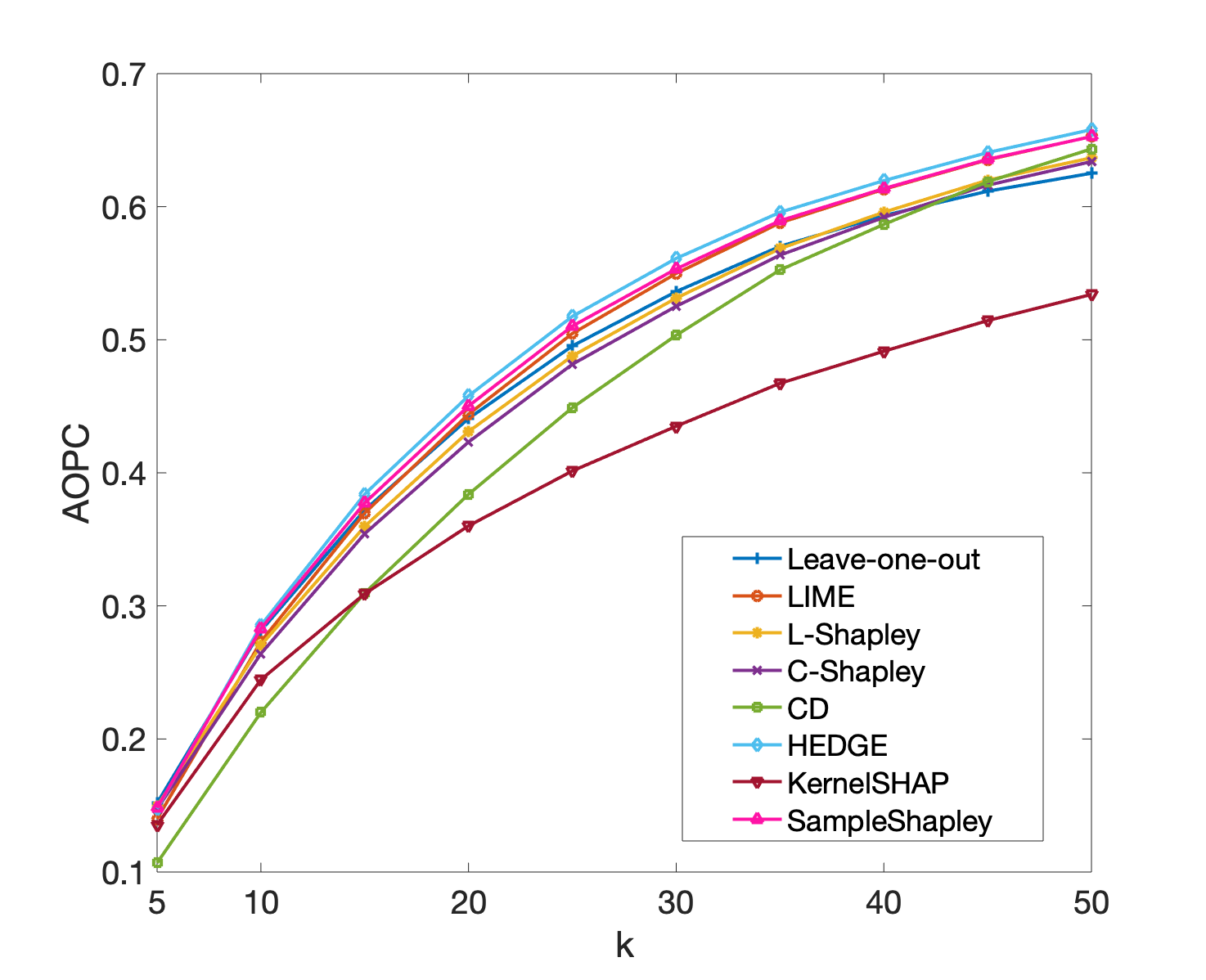
(a) AOPCs of LSTM on the SST dataset.

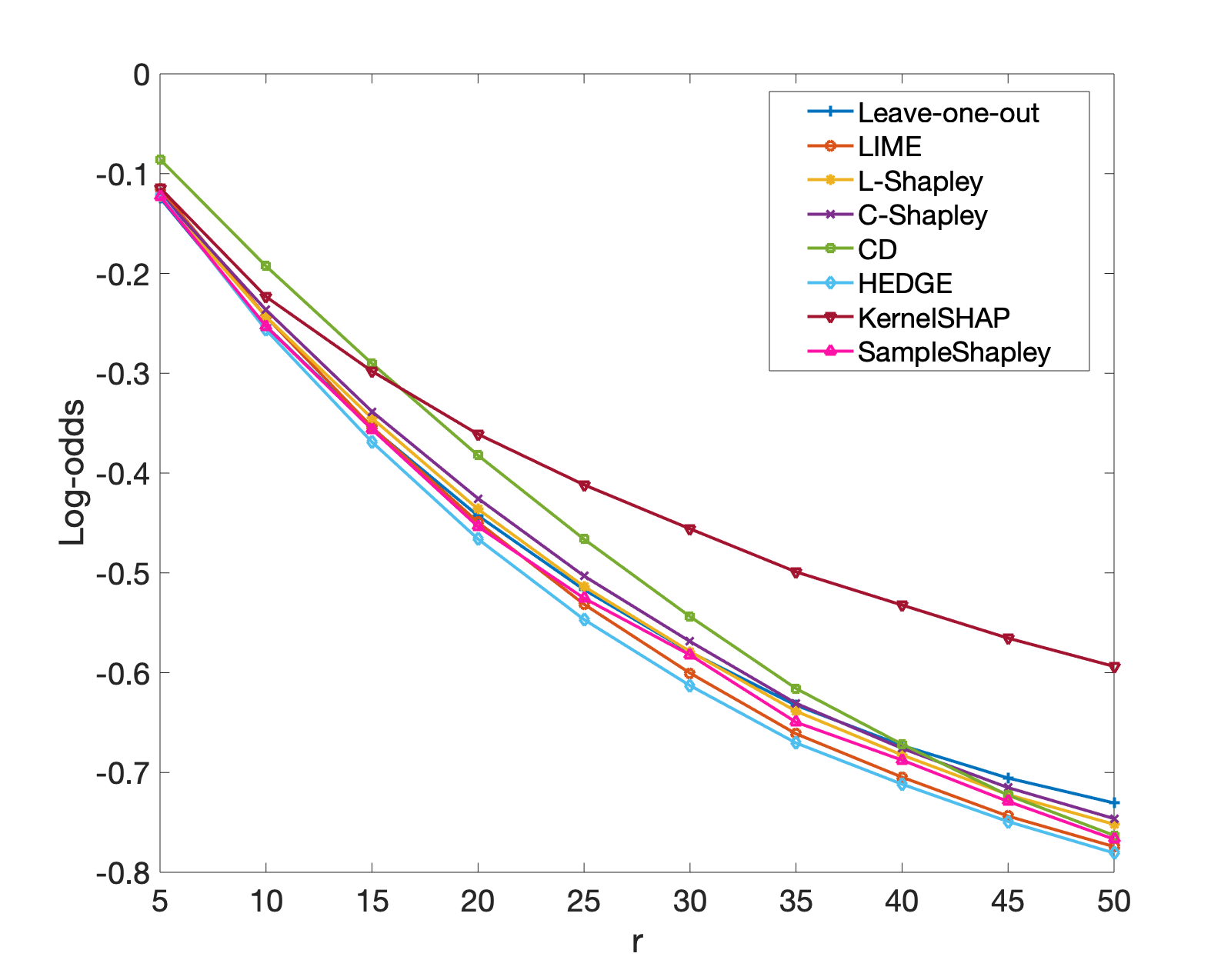
(b) Log-odds of LSTM on the SST dataset.

Figure 5: The AOPC and log-odds for LSTM on the SST dataset.

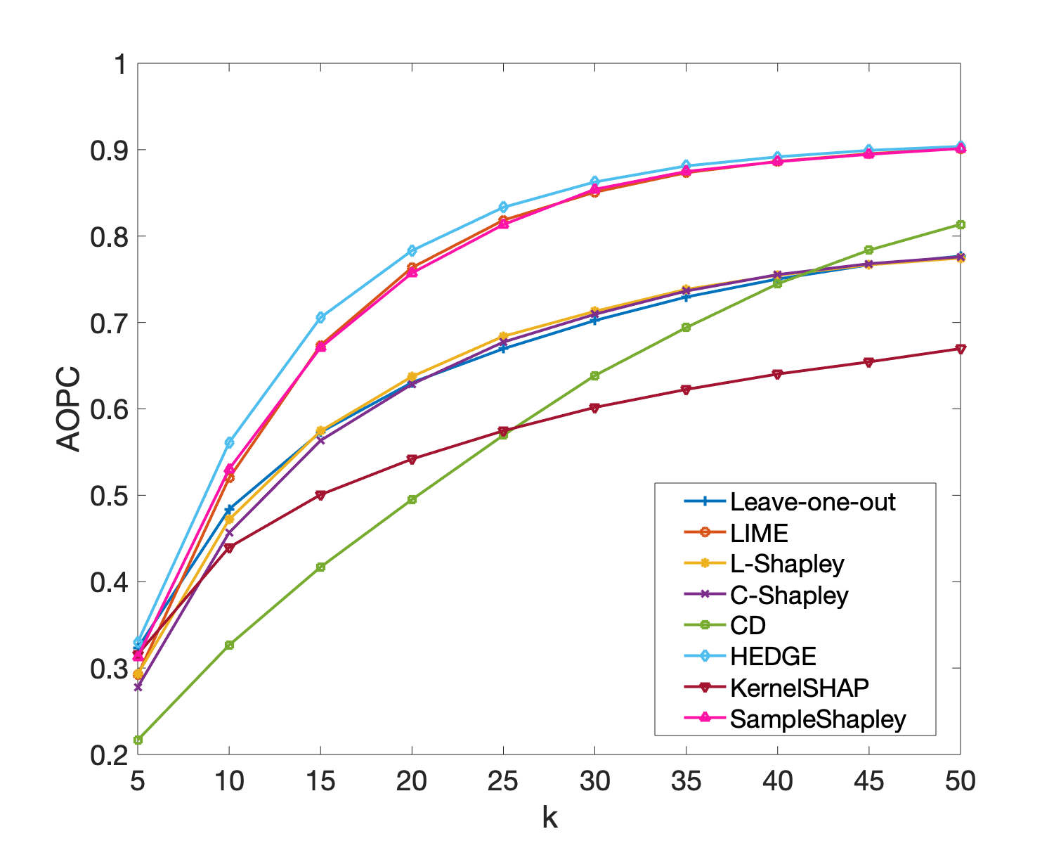
(a) AOPCs of LSTM on the IMDB dataset.

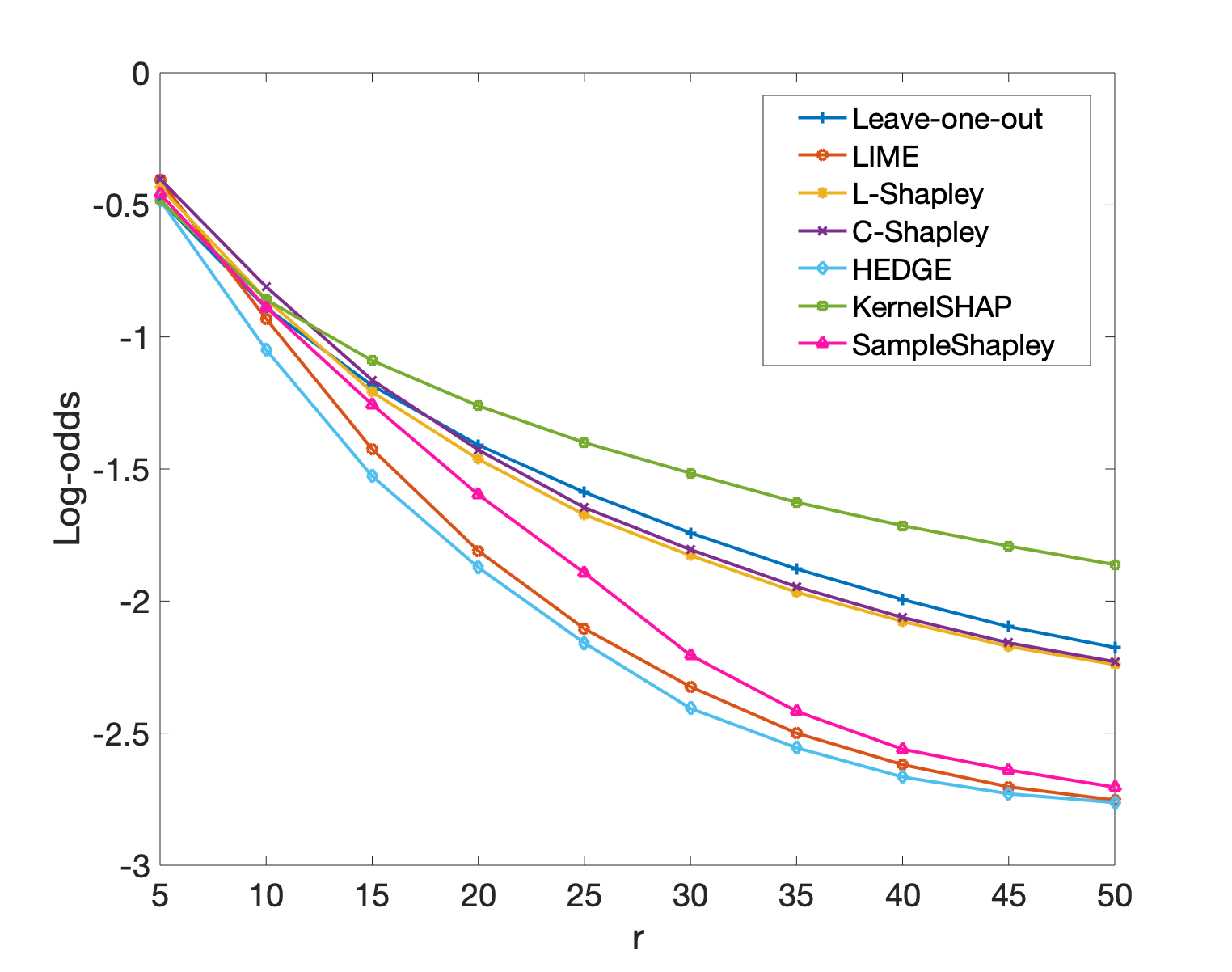
(b) Log-odds of LSTM on the IMDB dataset.

Figure 6: The AOPC and log-odds for LSTM on the IMDB dataset.

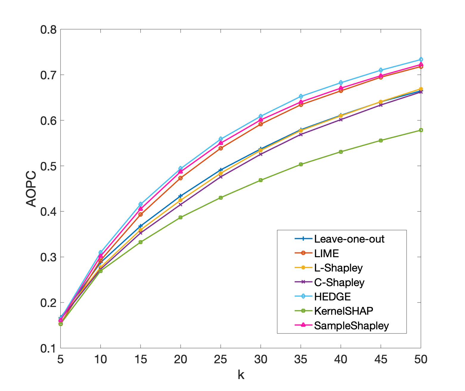
(a) AOPCs of CNN on the SST dataset.

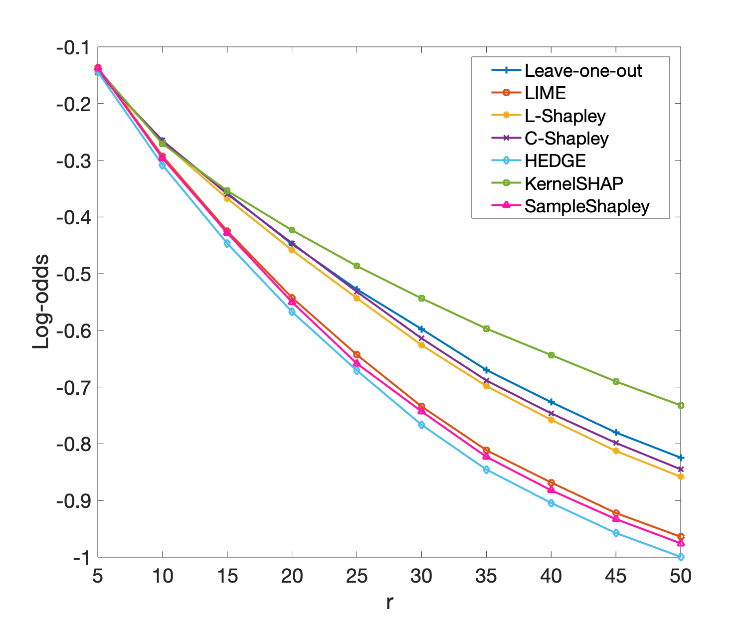
(b) Log-odds of CNN on the SST dataset.

Figure 7: The AOPC and log-odds for CNN on the SST dataset.

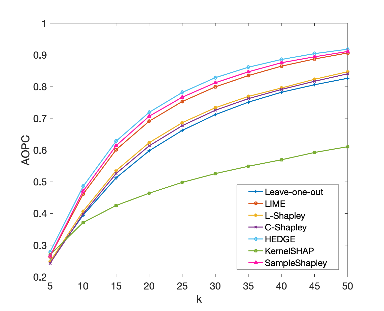
(a) AOPCs of CNN on the IMDB dataset.

(b) Log-odds of CNN on the IMDB dataset.

Figure 8: The AOPC and log-odds for CNN on the IMDB dataset.

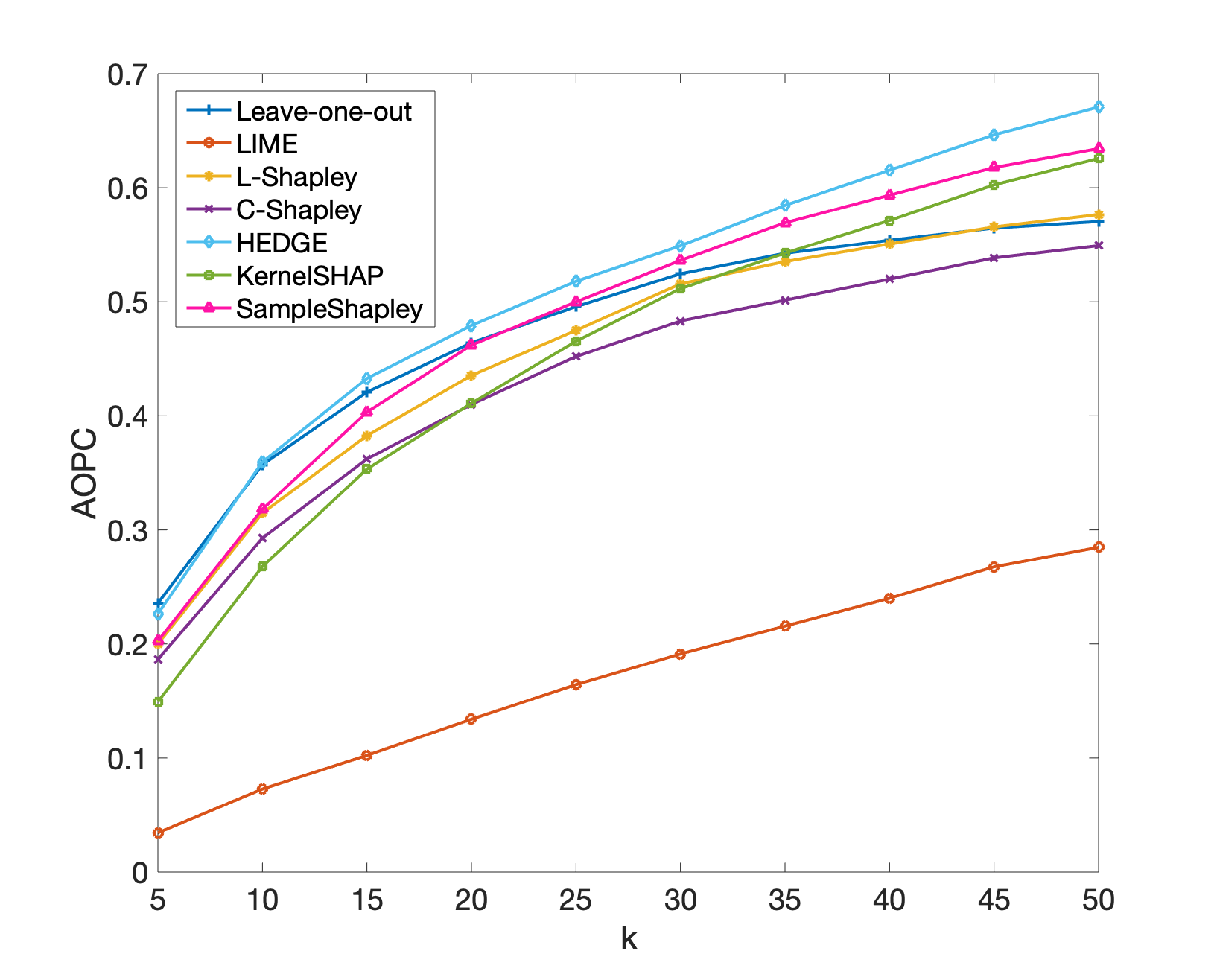
(a) AOPCs of BERT on the SST dataset.

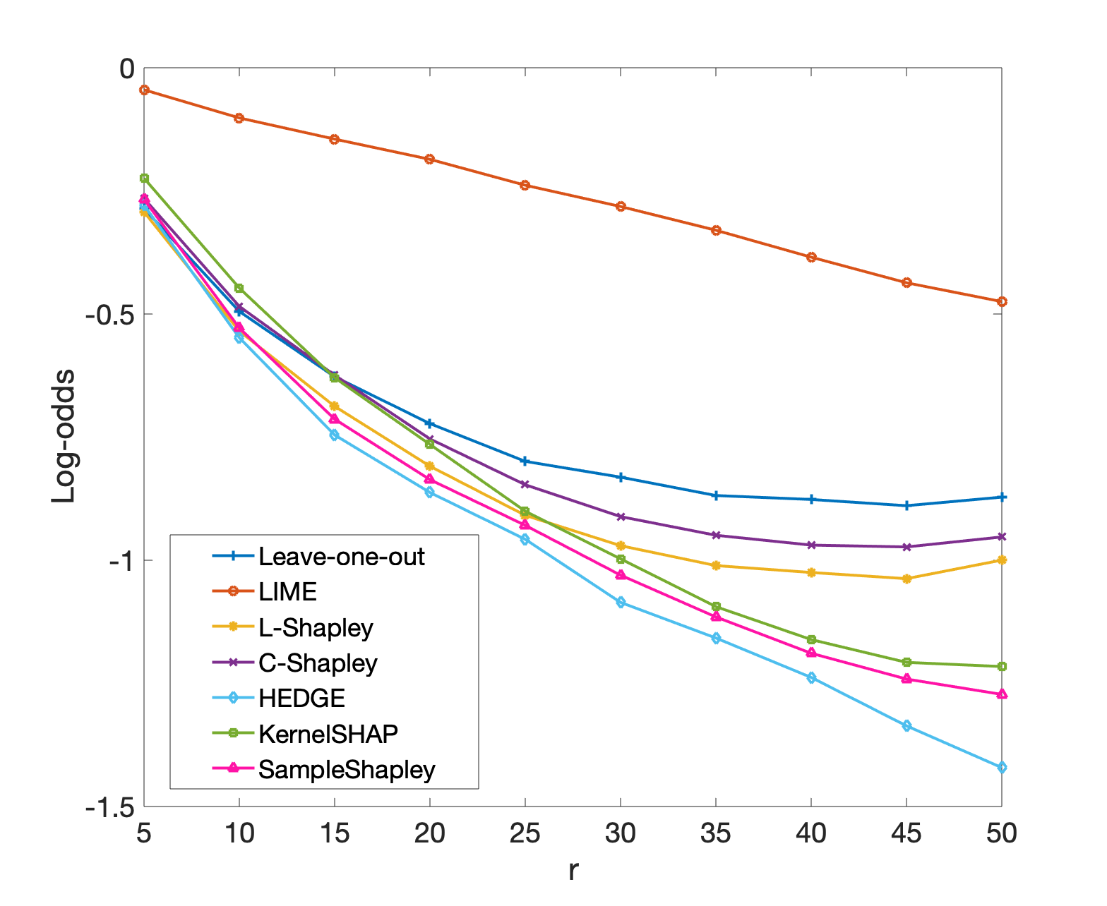
(b) Log-odds of BERT on the SST dataset.

Figure 9: The AOPC and log-odds for BERT on the SST dataset.

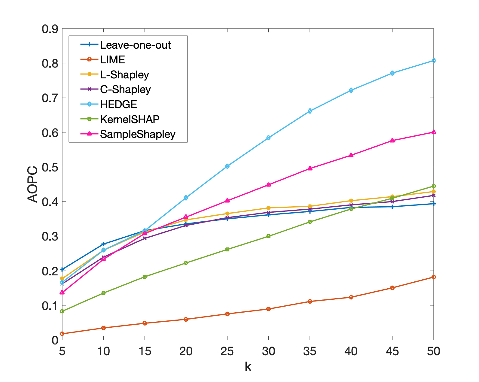
(a) AOPCs of BERT on the IMDB dataset.

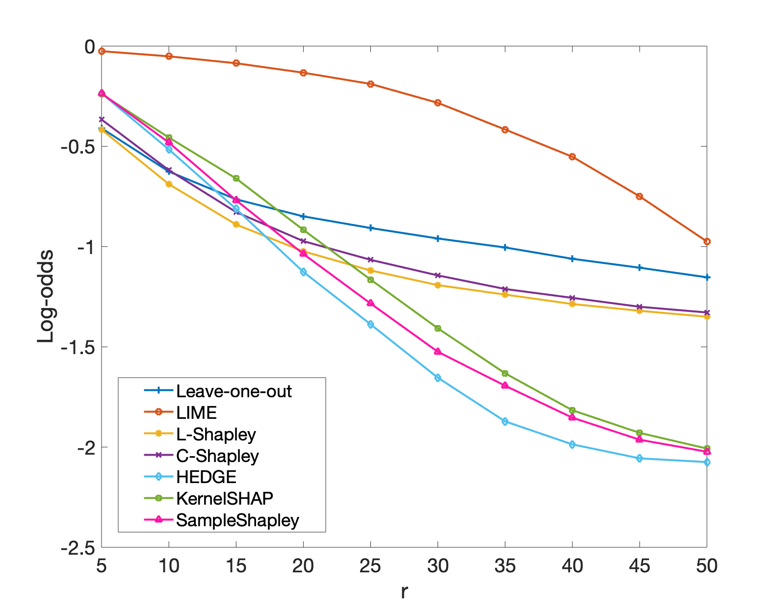
(b) Log-odds of BERT on the IMDB dataset.

Figure 10: The AOPC and log-odds for BERT on the IMDB dataset.

Appendix C Visualization of Hierarchical Interpretations

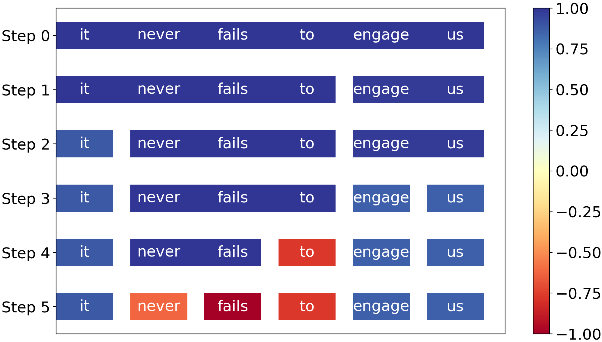
Figure 11: Hedge for BERT on a positive movie review from the SST dataset. BERT makes the correct prediction because it captures the interaction between never and fails.

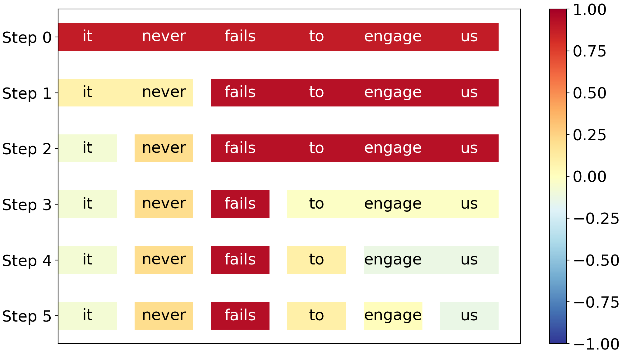
Figure 12: Hedge for LSTM on a positive movie review from the SST dataset. LSTM makes the wrong prediction because it misses the interaction between never and fails.

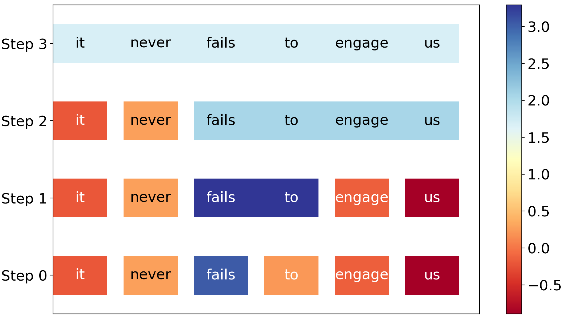
Figure 13: ACD for LSTM on a positive movie review from the SST dataset, on which LSTM makes wrong prediction.

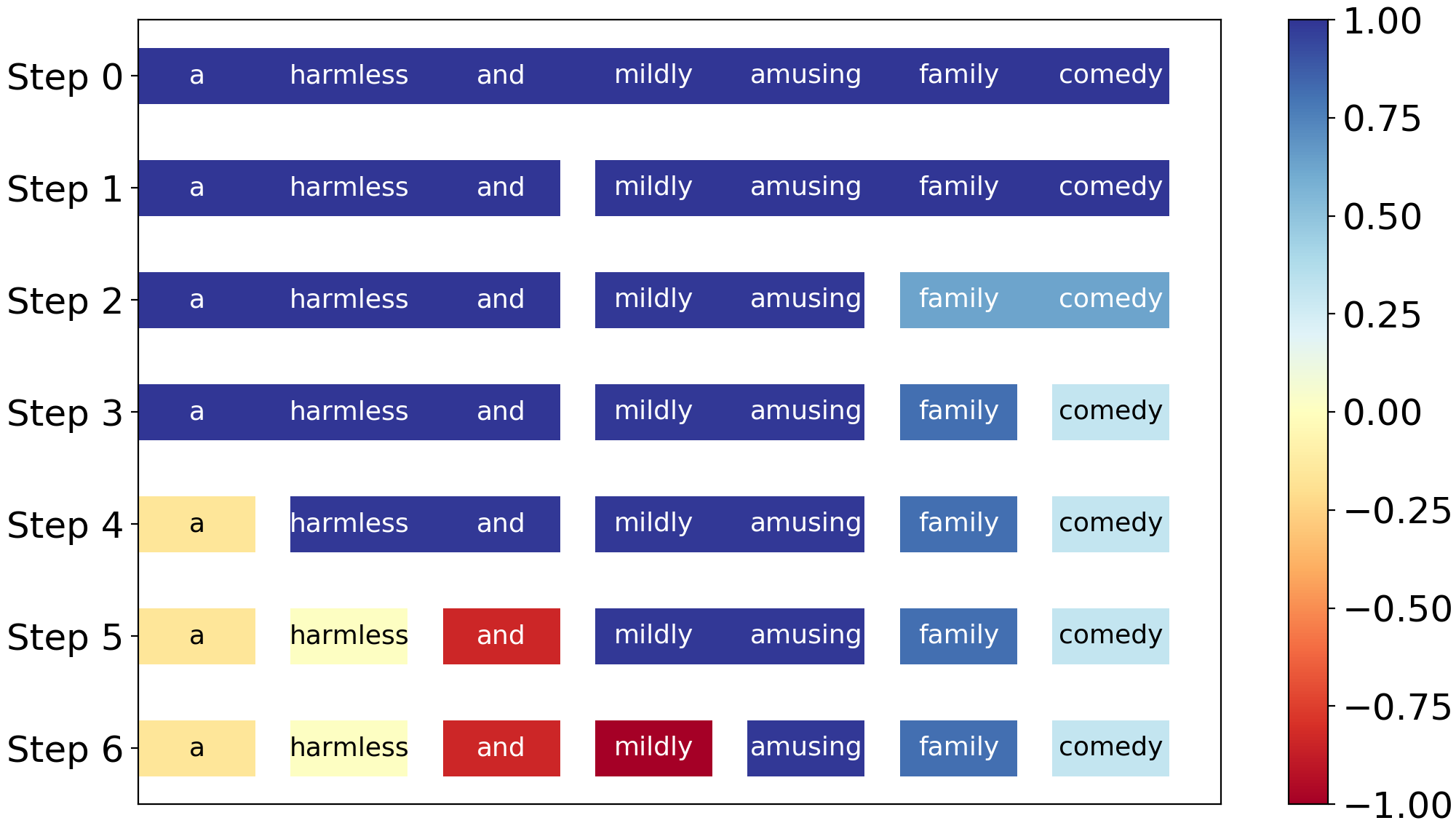
Figure 14: Hedge for BERT on a positive movie review from the SST dataset, on which BERT makes correct prediction.

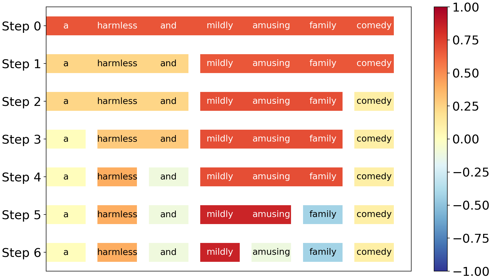
Figure 15: Hedge for LSTM on a positive movie review from the SST dataset, on which LSTM makes wrong prediction.

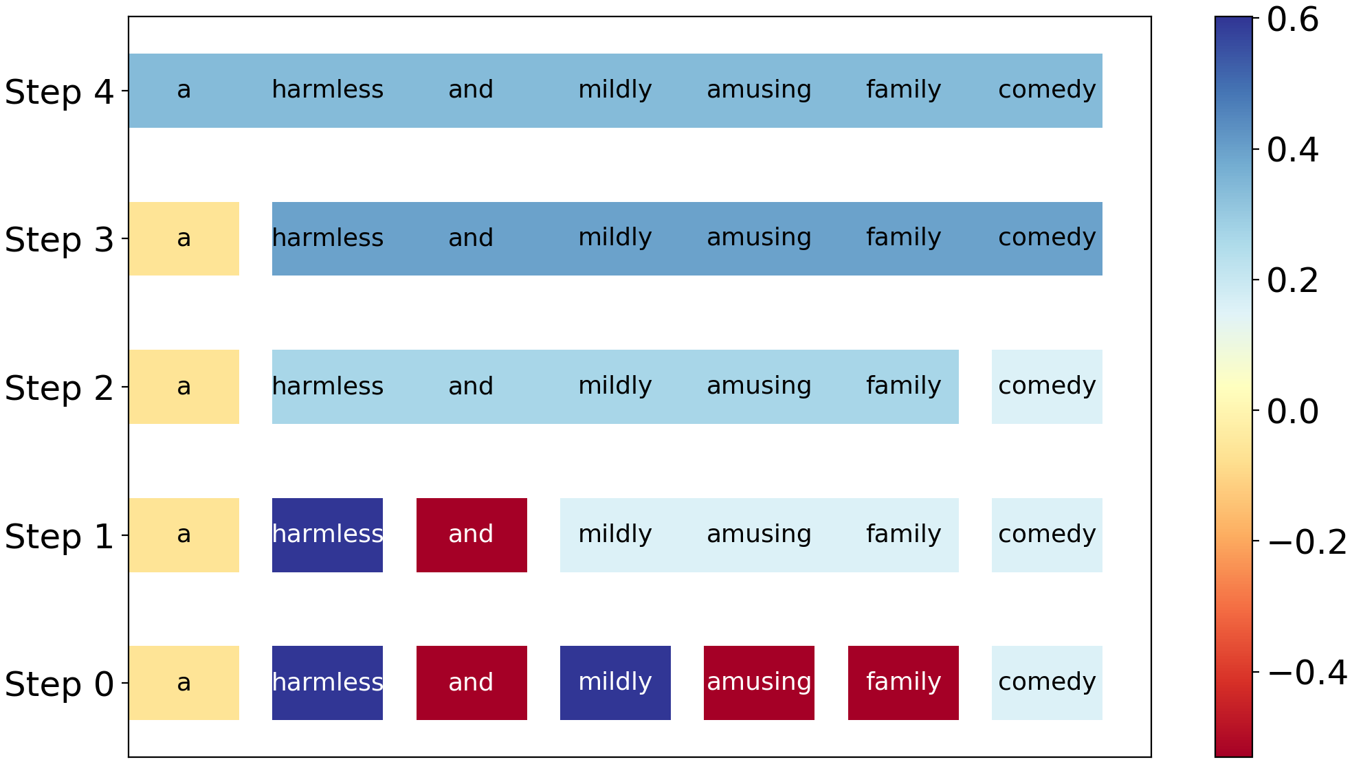
Figure 16: ACD for LSTM on a positive movie review from the SST dataset, on which LSTM makes wrong prediction.

Appendix D Human Evaluation Interface

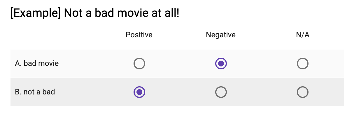
Figure 17: Interfaces of Amazon Mechanical Turk where annotators are asked to guess the model’s prediction based on different explanations.

References

- Alvarez-Melis and Jaakkola (2018) David Alvarez-Melis and Tommi S Jaakkola. 2018. Towards robust interpretability with self-explaining neural networks. In NeurIPS.
- Burns et al. (2018) Kaylee Burns, Aida Nematzadeh, Erin Grant, Alison Gopnik, and Tom Griffiths. 2018. Exploiting attention to reveal shortcomings in memory models. In Proceedings of the 2018 EMNLP Workshop BlackboxNLP: Analyzing and Interpreting Neural Networks for NLP, pages 378–380.
- Chen and Jordan (2019) Jianbo Chen and Michael I Jordan. 2019. Ls-tree: Model interpretation when the data are linguistic. arXiv preprint arXiv:1902.04187.
- Chen et al. (2018) Jianbo Chen, Le Song, Martin J Wainwright, and Michael I Jordan. 2018. L-shapley and c-shapley: Efficient model interpretation for structured data. arXiv preprint arXiv:1808.02610.
- Chen et al. (2016) Qian Chen, Xiaodan Zhu, Zhenhua Ling, Si Wei, Hui Jiang, and Diana Inkpen. 2016. Enhanced lstm for natural language inference. arXiv preprint arXiv:1609.06038.
- Datta et al. (2016) Anupam Datta, Shayak Sen, and Yair Zick. 2016. Algorithmic transparency via quantitative input influence: Theory and experiments with learning systems. In 2016 IEEE symposium on security and privacy (SP), pages 598–617. IEEE.
- Devlin et al. (2018) Jacob Devlin, Ming-Wei Chang, Kenton Lee, and Kristina Toutanova. 2018. Bert: Pre-training of deep bidirectional transformers for language understanding. arXiv preprint arXiv:1810.04805.
- Fujimoto et al. (2006) Katsushige Fujimoto, Ivan Kojadinovic, and Jean-Luc Marichal. 2006. Axiomatic characterizations of probabilistic and cardinal-probabilistic interaction indices. Games and Economic Behavior, 55(1):72–99.
- Ghaeini et al. (2018) Reza Ghaeini, Xiaoli Z Fern, and Prasad Tadepalli. 2018. Interpreting recurrent and attention-based neural models: a case study on natural language inference. arXiv preprint arXiv:1808.03894.
- Godin et al. (2018) Fréderic Godin, Kris Demuynck, Joni Dambre, Wesley De Neve, and Thomas Demeester. 2018. Explaining character-aware neural networks for word-level prediction: Do they discover linguistic rules? arXiv preprint arXiv:1808.09551.
- Grabisch (1997) Michel Grabisch. 1997. K-order additive discrete fuzzy measures and their representation. Fuzzy sets and systems, 92(2):167–189.
- Hechtlinger (2016) Yotam Hechtlinger. 2016. Interpretation of prediction models using the input gradient. arXiv preprint arXiv:1611.07634.
- Hochreiter and Schmidhuber (1997) Sepp Hochreiter and Jürgen Schmidhuber. 1997. Long short-term memory. Neural computation, 9(8):1735–1780.
- Howard and Ruder (2018) Jeremy Howard and Sebastian Ruder. 2018. Universal language model fine-tuning for text classification. arXiv preprint arXiv:1801.06146.
- Hu et al. (2016) Ronghang Hu, Huazhe Xu, Marcus Rohrbach, Jiashi Feng, Kate Saenko, and Trevor Darrell. 2016. Natural language object retrieval. In Proceedings of the IEEE Conference on Computer Vision and Pattern Recognition, pages 4555–4564.
- Jacovi et al. (2018) Alon Jacovi, Oren Sar Shalom, and Yoav Goldberg. 2018. Understanding convolutional neural networks for text classification. arXiv preprint arXiv:1809.08037.
- Jin et al. (2019) Xisen Jin, Junyi Du, Zhongyu Wei, Xiangyang Xue, and Xiang Ren. 2019. Towards hierarchical importance attribution: Explaining compositional semantics for neural sequence models.
- Jumelet and Hupkes (2018) Jaap Jumelet and Dieuwke Hupkes. 2018. Do language models understand anything? on the ability of lstms to understand negative polarity items. arXiv preprint arXiv:1808.10627.
- Kim (2014) Yoon Kim. 2014. Convolutional neural networks for sentence classification. arXiv preprint arXiv:1408.5882.
- Kononenko et al. (2010) Igor Kononenko et al. 2010. An efficient explanation of individual classifications using game theory. Journal of Machine Learning Research, 11(Jan):1–18.
- Lee et al. (2017) Jaesong Lee, Joong-Hwi Shin, and Jun-Seok Kim. 2017. Interactive visualization and manipulation of attention-based neural machine translation. In Proceedings of the 2017 Conference on Empirical Methods in Natural Language Processing: System Demonstrations, pages 121–126.
- Lei et al. (2016) Tao Lei, Regina Barzilay, and Tommi Jaakkola. 2016. Rationalizing neural predictions. In Proceedings of the 2016 Conference on Empirical Methods in Natural Language Processing, pages 107–117.
- Li et al. (2016) Jiwei Li, Will Monroe, and Dan Jurafsky. 2016. Understanding neural networks through representation erasure. arXiv preprint arXiv:1612.08220.
- Lipton (2016) Zachary C Lipton. 2016. The mythos of model interpretability. arXiv preprint arXiv:1606.03490.
- Lundberg et al. (2018) Scott M Lundberg, Gabriel G Erion, and Su-In Lee. 2018. Consistent individualized feature attribution for tree ensembles. arXiv preprint arXiv:1802.03888.
- Lundberg and Lee (2017) Scott M Lundberg and Su-In Lee. 2017. A unified approach to interpreting model predictions. In Advances in Neural Information Processing Systems, pages 4765–4774.
- Maas et al. (2011) Andrew L Maas, Raymond E Daly, Peter T Pham, Dan Huang, Andrew Y Ng, and Christopher Potts. 2011. Learning word vectors for sentiment analysis. In Proceedings of the 49th annual meeting of the association for computational linguistics: Human language technologies-volume 1, pages 142–150. Association for Computational Linguistics.
- Mikolov et al. (2013) Tomas Mikolov, Ilya Sutskever, Kai Chen, Greg S Corrado, and Jeff Dean. 2013. Distributed representations of words and phrases and their compositionality. In Advances in neural information processing systems, pages 3111–3119.
- Murdoch et al. (2018) W James Murdoch, Peter J Liu, and Bin Yu. 2018. Beyond word importance: Contextual decomposition to extract interactions from lstms. arXiv preprint arXiv:1801.05453.
- Nguyen (2018) Dong Nguyen. 2018. Comparing automatic and human evaluation of local explanations for text classification. In Proceedings of the 2018 Conference of the North American Chapter of the Association for Computational Linguistics: Human Language Technologies, Volume 1 (Long Papers), pages 1069–1078.
- Owen (1972) Guillermo Owen. 1972. Multilinear extensions of games. Management Science, 18(5-part-2):64–79.
- Peters et al. (2018) Matthew E Peters, Mark Neumann, Mohit Iyyer, Matt Gardner, Christopher Clark, Kenton Lee, and Luke Zettlemoyer. 2018. Deep contextualized word representations. arXiv preprint arXiv:1802.05365.
- Plumb et al. (2018) Gregory Plumb, Denali Molitor, and Ameet S Talwalkar. 2018. Model agnostic supervised local explanations. In Advances in Neural Information Processing Systems, pages 2515–2524.
- Ribeiro et al. (2016) Marco Tulio Ribeiro, Sameer Singh, and Carlos Guestrin. 2016. Why should i trust you?: Explaining the predictions of any classifier. In Proceedings of the 22nd ACM SIGKDD international conference on knowledge discovery and data mining, pages 1135–1144. ACM.
- Samek et al. (2016) Wojciech Samek, Alexander Binder, Grégoire Montavon, Sebastian Lapuschkin, and Klaus-Robert Müller. 2016. Evaluating the visualization of what a deep neural network has learned. IEEE transactions on neural networks and learning systems, 28(11):2660–2673.
- Serrano and Smith (2019) Sofia Serrano and Noah A Smith. 2019. Is attention interpretable? arXiv preprint arXiv:1906.03731.
- Shapley (1953) Lloyd S Shapley. 1953. A value for n-person games. Contributions to the Theory of Games, 2(28).
- Shrikumar et al. (2017) Avanti Shrikumar, Peyton Greenside, and Anshul Kundaje. 2017. Learning important features through propagating activation differences. In Proceedings of the 34th International Conference on Machine Learning-Volume 70, pages 3145–3153. JMLR. org.
- Singh et al. (2019) Chandan Singh, W. James Murdoch, and Bin Yu. 2019. Hierarchical interpretations for neural network predictions. In International Conference on Learning Representations.
- Socher et al. (2013) Richard Socher, Alex Perelygin, Jean Wu, Jason Chuang, Christopher D Manning, Andrew Ng, and Christopher Potts. 2013. Recursive deep models for semantic compositionality over a sentiment treebank. In Proceedings of the 2013 conference on empirical methods in natural language processing, pages 1631–1642.
- Štrumbelj and Kononenko (2014) Erik Štrumbelj and Igor Kononenko. 2014. Explaining prediction models and individual predictions with feature contributions. Knowledge and information systems, 41(3):647–665.
- Sundararajan et al. (2017) Mukund Sundararajan, Ankur Taly, and Qiqi Yan. 2017. Axiomatic attribution for deep networks. In Proceedings of the 34th International Conference on Machine Learning-Volume 70, pages 3319–3328. JMLR. org.
- Tsang et al. (2018) Michael Tsang, Youbang Sun, Dongxu Ren, and Yan Liu. 2018. Can i trust you more? model-agnostic hierarchical explanations. arXiv preprint arXiv:1812.04801.