Unstructured space-time finite element methods for optimal control of parabolic equations

Abstract

This work presents and analyzes space-time finite element methods on fully unstructured simplicial space-time meshes for the numerical solution of parabolic optimal control problems. Using Babuška’s theorem, we show well-posedness of the first-order optimality systems for a typical model problem with linear state equations, but without control constraints. This is done for both continuous and discrete levels. Based on these results, we derive discretization error estimates. Then we consider a semilinear parabolic optimal control problem arising from the Schlögl model. The associated nonlinear optimality system is solved by Newton’s method, where a linear system, that is similar to the first-order optimality systems considered for the linear model problems, has to be solved at each Newton step. We present various numerical experiments including results for adaptive space-time finite element discretizations based on residual-type error indicators. In the last two examples, we also consider semilinear parabolic optimal control problems with box constraints imposed on the control.

Keywords: Parabolic optimal control problems, space-time finite element methods, discretization error estimates, linear parabolic equations, semilinear parabolic equations.

2010 MSC: 49J20, 35K20, 65M60, 65M50, 65M15, 65Y05

1 Introduction

In this paper, we apply continuous space-time finite element methods on fully unstructured simplicial space-time meshes to the numerical solution of optimal control problems for linear and semilinear parabolic equations. More precisely, we treat the corresponding parabolic forward-backward optimality systems at once. In this way, we are able to apply the semismooth Newton method for the optimal control of semilinear state equations and for problems with pointwise control constraints. In particular, this is a challenge for our examples with reaction-diffusion equations that develop wave-type solutions. We present an error analysis for problems with a linear state equation without control constraints. However, our numerical examples confirm that the continuous space-time finite element approach works also well for problems with semilinear equations and under additional pointwise control constraints.

Continuous space-time finite element methods (FEM) for solving parabolic initial-boundary value problems (IBVP) on fully unstructured simplicial space-time meshes have recently been studied from a mathematical point of view, e.g., in [6, 33, 41], and have been used in engineering applications; see, e.g., [8, 27]. We also refer the reader to the recent review article [43] on this topic and the related references therein. This space-time approach considers the time variable as just another variable in contrast to the classical time-stepping methods or to the more recent, but closely related time discontinuous Galerkin (dG) or discontinuous Petrov-Galerkin (dPG) methods operating on time slices or slabs. There is a huge amount of papers on these methods. Here we only refer to the classical monograph [44] and to the survey articles [19, 43]. The fully unstructured space-time FEM is obviously more flexible with respect to approximation, adaptivity, and parallelization than time-stepping methods. Moving interfaces or spatial domains are fixed geometric objects in the space-time domain. However, we have to solve one large-scale system of linear or non-linear algebraic equations at once instead of many smaller systems sequentially arising at each time step. This may be seen as a disadvantage when using a sequential computation on a standard computer (desktop or laptop) with one or only a few cores. However, this is definitely a huge advantage on massively parallel computers. Even on a standard computer, simultaneous space-time adaptivity can dramatically reduce the complexity as our numerical experiments presented in this paper show. Indeed, we are able to solve optimal control problems for linear and semilinear parabolic reaction-diffusion equations in two-dimensional spatial domains fast and with high accuracy on standard desktops or even laptops. We should underline that all of our numerical experiments were performed on a laptop or desktop computer.

An optimal control problem for a parabolic partial differential equation leads to necessary optimality conditions that include a coupled system consisting of the state equation being forward in time, and the adjoint equation (co-state equation) that is directed backward in time, see, e.g., [36] or [46]. The numerical solution of this forward-backward system is very demanding, because this cannot easily be done by standard time-stepping methods or time-slice dG or dPG methods in an efficient way. We here only mention the works by Meidner and Vexler [37, 38] for optimal error estimates of advanced time-stepping dG methods in the optimal control of parabolic PDEs. Therefore, various other methods were applied for spatial dimensions larger than one, for instance, gradient type methods that proceed by sequentially solving forward and backward equations [25, 46]. Moreover, several techniques were used that lower the dimension of the discretized equations to be solved. We mention multigrid methods, Hackbusch [23], and cf. also the monograph by Borzi and Schulz [10]; model order reduction by proper orthogonal decomposistion (POD), Alla and Volkwein [1], Kunisch, Volkwein and Xie [29]; wavelet decomposition, Kunoth [30]; tensor product approximations [12, 22, 28, 34]; or adaptive methods based on goal-oriented error estimators, Becker et al. [7], Hintermüller et al [24]. Gong, Hinze and Zhou [20] propose to solve a higher-order optimality system (second-order in time and fourth-order in space) by means of a time-slice discretization. A detailed survey on all related literature would exceed the scope of this paper. Hence, we confine ourselves to the papers mentioned above, and the references therein.

In contrast to these approaches, we apply fully unstructured space-time FEM to the numerical solution of optimal control problems for linear and semilinear parabolic partial differential equations. The fully unstructured space-time methods are especially suited for a forward-backward system since it is one system of two coupled PDEs where the time is just another variable.

We start our investigation with a the standard space-time tracking optimal control problem subject to a linear parabolic IBVP. The well-posedness of the optimality system and of the discretized optimality system is studied by Babuška’s theorem. In particular, the discrete inf-sup (stability) condition leads to asymptotically optimal discretization error estimates.

For problems with a semilinear state equation or pointwise control constraints, we apply the semismooth Newton method, the currently most popular and powerful numerical technique for solving optimal control problems for PDEs; we refer to Ito and Kunisch [26]. In this Newton-type method, a sequence of forward-backward equations must be solved that easily exceed the storage capacity of standard computers, if the space dimension is larger than one. Parallel-in-time numerical techniques such as parareal methods, cf. Lions et. al. [35], Ulbrich [47], see also Gander [19], can also overcome this difficulty. However, they are not easy to implement. In this context, we also mention Götschel and Minion [21], who apply parallel-in-time methods to the optimal control of the 3D heat equation and the 1D Nagumo equation.

In our examples, the level of difficulty is even higher, because our reaction-diffusion equations exhibit wave type solutions such as traveling wave fronts, spiral waves, or scroll rings. We refer, e.g., to Casas et. al. [14, 15, 16], where optimal control problems for FitzHugh-Nagumo or Schlögl (Nagumo) equations were solved in space dimensions one and two. Only in the spatially one-dimensional case, the semismooth Newton method was applied, cf. [15], while two-dimensional problems were tackled by a nonlinear conjugate gradient optimization method, partially invoking a model-predictive approximation. In contrast to the papers mentioned above, we directly solve the nonlinear optimality systems by the Newton or semismooth Newton method. Finally, in each iteration, we solve one system of linear or non-linear algebraic equations.

The rest of the paper is structured as follows. In Section 2, we introduce some notation and state some preliminary results on the solvability and numerical analysis of the parabolic initial-boundary value problem that serves as state equation in the optimal control problem studied in Section 3. In Section 4, we consider the optimal control of semilinear parabolic initial-boundary value problem without and with pointwise box constraints on the control. We provide and discuss typical numerical examples for all optimal control problems investigated in the paper. Finally, some conclusions are drawn in Section 5.

2 Preliminaries

The state problem, that appears as constraint in the optimal control problems, is given by the linear parabolic IBVP

$$\partial_{t}u-\Delta_{x}u=z\textup{ in }Q,\quad u=0\textup{ on }\Sigma,\quad u=0\textup{ on }\Sigma_{0},$$ (1)

where $Q:=\Omega\times(0,T)$, $\Sigma:=\partial\Omega\times(0,T)$, $\Sigma_{0}:=\Omega\times\{0\}$. The spatial computational domain $\Omega\subset\mathbb{R}^{d}$, $d=1,2,3$, is supposed to be bounded and Lipschitz, $T>0$ is the final time, $\partial_{t}$ denotes the partial time derivative, $\Delta_{x}=\sum_{i=1}^{d}\partial^{2}_{x_{i}}$ is the spatial Laplacian, and the source term $z$ on the right-hand side of the parabolic PDE serves as control. For simplicity, we consider homogeneous initial and boundary conditions only. It is clear that this simple model problem can be replaced by more advanced parabolic IBVPs as they appear in many practical applications such as instationary heat conduction, instationary diffusion, 2D eddy current simulation, tumor grow, or after Newton linearization of nonlinear parabolic IBVPs as considered in Section 4. The weak solvability of such kind of parabolic IBVPs was studied in space-time Sobolev spaces by Ladyzhenskaya and co-workers [31, 32], and in Bochner spaces of abstract functions, mapping the time interval $(0,T)$ to some Hilbert or Banach space, by Lions [36], see also [48]. Following the latter approach, the standard weak formulation of the IBVP (1) in Bochner spaces of abstract functions reads as follows: Given $z\in Y^{*}$, find $u\in X_{0}$ such that

$$b(u,v)=\langle z,v\rangle_{Q},\quad\forall v\in Y,$$ (2)

with the bilinear form $b(\cdot,\cdot):X_{0}\times Y\to\mathbb{R}$,

$$b(u,v):=\int_{Q}\Big{[}\partial_{t}u\,v+\nabla_{x}u\cdot\nabla_{x}v\Big{]}\,dx\,dt,\quad\forall(u,v)\in X_{0}\times Y,$$ (3)

and the linear form $\langle z,\cdot\rangle_{Q}:Y\to\mathbb{R}$ with the duality pairing

$$\langle z,q\rangle_{Q}:=\int_{Q}z\,v\,dx\,dt,\quad\forall v\in Y,$$ (4)

as extension of the inner product in $L^{2}(Q)$. Similarly, the first integral in (3) has to be understood as duality pairing as well. The Bochner spaces $X_{0}$ and $Y$ are specified as follows:

$$X_{0} := L^{2}(0,T;H_{0}^{1}(\Omega))\cap H_{0,}^{1}(0,T;H^{-1}(\Omega))$$

$$= \Big{\{}v\in L^{2}(0,T;H_{0}^{1}(\Omega)):\partial_{t}v\in L^{2}(0,T;H^{-1}(\Omega)),\,v=0\mbox{ on }\Sigma_{0}\Big{\}},$$

$$Y := L^{2}(0,T;H_{0}^{1}(\Omega)),\qquad Y^{*}:=L^{2}(0,T;H^{-1}(\Omega)),$$

where $H_{0}^{1}(\Omega):=\{v\in H^{1}(\Omega):\,v=0\mbox{ on }\partial\Omega\}$, and $H^{-1}(\Omega):=H_{0}^{1}(\Omega)^{*}$. Note that we have $X_{0}=\{v\in W(0,T):\,v=0\mbox{ on }\Sigma_{0}\}$ as used in [36]. The related norms are given by

$$\|u\|_{X_{0}} := \Big{(}\|\partial_{t}u\|^{2}_{L^{2}(0,T;H^{-1}(\Omega))}+\|\nabla_{x}u\|^{2}_{L^{2}(Q)}\Big{)}^{1/2},$$

$$\|v\|_{Y} := \|\nabla_{x}v\|_{L^{2}(Q)},$$

$$\|\partial_{t}u\|_{Y^{*}} = \|\partial_{t}u\|_{L^{2}(0,T;H^{-1}(\Omega))}=\|\nabla_{x}w_{u}\|_{L^{2}(Q)}=\|w_{u}\|_{Y},$$

and where $w_{u}\in Y$ is the unique solution of the variational formulation

$$\int_{Q}\nabla_{x}w_{u}\cdot\nabla_{x}v\,dx\,dt=\langle\partial_{t}u,v\rangle_{Q},\quad\forall v\in Y;$$ (5)

see [41]. In fact, we have

$$\|u\|_{X_{0}}=\Big{[}\|w_{u}\|_{Y}^{2}+\|u\|_{Y}^{2}\Big{]}^{1/2}.$$

The well-posedness of variational problems such as (2) can be investigated by the Nec̆as-Babuška theorem [4, 40] that is sometimes also called the Banach-Nec̆as-Babuška theorem [18] or the Babuška-Aziz theorem [5], see also [11]. This theorem states that the operator $B:X_{0}\to Y^{*}$ generated by the bilinear form $b(\cdot,\cdot)$ is an isomorphism if and only if the following three conditions are fulfilled:

1. boundedness (continuity) of $b(\cdot,\cdot)$, i.e., there exists a positive constant $\beta_{1}$:

   $$|b(u,v)|\leq\beta_{1}\,\|u\|_{X_{0}}\|v\|_{Y},\quad\forall(u,v)\in X_{0}\times Y;$$ (6)

2. inf-sup (stability) condition (surjectivity of $B^{*}$), i.e., there exists a positive constant $\beta_{2}$ such that

   $$\inf\limits_{0\neq u\in X_{0}}\sup\limits_{0\neq v\in Y}\frac{b(u,v)}{\|u\|_{X_{0}}\|v\|_{Y}}\geq\beta_{2};$$ (7)

3. injectivity of $B^{*}$:

   $$\forall v\in Y\setminus\{0\}\;\exists\widetilde{u}\in X_{0}:\;b(\widetilde{u},v)\neq 0.$$ (8)

It is easy to show that the bilinear form (3) is bounded with $\beta_{1}=\sqrt{2}$. The inf-sup condition (7) follows from [41, Theorem 2.1] with the stability constant $\beta_{2}=1/(2\sqrt{2})$. To prove (8), for $v\in Y\setminus\{0\}$, we choose

$$\widetilde{u}(x,t)=\int_{0}^{t}v(x,s)\,ds,\quad(x,t)\in Q.$$

By definition, we have $\widetilde{u}\in X_{0}$, and

$$b(\widetilde{u},v)=\|v\|^{2}_{L^{2}(Q)}+\frac{1}{2}\,\|\nabla_{x}\widetilde{u}(T)\|^{2}_{L^{2}(\Omega)}>0.$$

Therefore, by the Nec̆as-Babuška theorem, the variational problem (2) is well-posed.

For the finite element discretization of the variational formulation (2), we introduce conforming space-time finite element spaces $X_{0,h}\subset X_{0}$ and $Y_{h}\subset Y$, where we assume $X_{0,h}\subseteq Y_{h}$. In particular, we may use $X_{0,h}=Y_{h}=S_{h}^{1}(Q_{h})\cap X_{0}$ spanned by continuous and piecewise linear basis functions which are defined with respect to some admissible decomposition $\mathcal{T}_{h}(Q)$ of the space-time domain $Q$ into shape regular simplicial finite elements $\tau_{\ell}$, and which are zero at the initial time $t=0$ and at the lateral boundary $\Sigma$, where $h$ denotes a suitable mesh-size parameter, see, e.g., [11, 18, 41]. Then the finite element approximation of (2) is to find $u_{h}\in X_{0,h}$ such that

$$b(u_{h},v_{h})=\langle z,v_{h}\rangle_{Q},\quad\forall v_{h}\in Y_{h}.$$ (9)

When replacing (5) by its finite element approximation to find $w_{u,h}\in Y_{h}$ such that

$$\int_{Q}\nabla_{x}w_{u,h}\cdot\nabla_{x}v_{h}\,dx\,dt=\int_{Q}\partial_{t}u\,v_{h}\,dx\,dt,\quad\forall v_{h}\in Y_{h},$$ (10)

we can define a discrete norm

$$\|u\|_{X_{0,h}}\,:=\Big{[}\|w_{u,h}\|_{Y}^{2}+\|u\|_{Y}^{2}\Big{]}^{1/2}\,.$$

Due to the definition of $w_{u,h}$ as solution of the variational formulation (10), we conclude

$$\|w_{u,h}\|_{Y}\leq\|w_{u}\|_{Y}\quad\mbox{for all}\;u\in X_{0},$$ (11)

while the opposite inequality is in general not true. As in the continuous case, see (7), we can prove a discrete inf-sup condition, see [41, Theorem 3.1],

$$\frac{1}{2\sqrt{2}}\,\|u_{h}\|_{X_{0,h}}\leq\sup\limits_{0\neq v_{h}\in Y_{h}}\frac{b(u_{h},v_{h})}{\|v_{h}\|_{Y}},\quad\forall u_{h}\in X_{0,h}.$$ (12)

Hence, from the discrete version of Nec̆as-Babuška’s theorem, we conclude unique solvability of the Galerkin scheme (9). Furthermore, we obtain the following quasi-optimal error estimate, see [41, Theorem 3.2]:

$$\|u-u_{h}\|_{X_{0,h}}\leq 5\inf\limits_{z_{h}\in X_{0,h}}\|u-z_{h}\|_{X_{0}}\,.$$ (13)

In particular, when assuming $u\in H^{2}(Q)$, this finally results in the energy error estimate, see [41, Theorem 3.3],

$$\|u-u_{h}\|_{L^{2}(0,T;H^{1}_{0}(\Omega))}\leq c\,h\,|u|_{H^{2}(Q)}\,.$$ (14)

Once the basis is chosen, the finite element scheme (9) is nothing but a huge linear system of the form

$$K_{h}\underline{u}_{h}=\underline{f}_{h}$$ (15)

with a positive definite, but non-symmetric system matrix $K_{h}$ that can be generated together with the right-hand side $\underline{f}_{h}$ similar as in the elliptic case. The linear system (15) can efficiently be solved by means of the preconditioned GMRES method, see [42, 43], where Algebraic Multigrid (AMG) preconditioning is used. We also use AMG preconditioned GMRES as solver in all numerical experiments presented in this paper. It is clear that the unstructured space-time approach to optimal control problems presented in this paper allows full space-time adaptivity and parallelization.

3 Space-time tracking

3.1 The model problem

For a given target function $u_{d}\in L^{2}(Q)$ and a regularization parameter $\varrho>0$, we consider the minimization of the cost functional

$${\mathcal{J}}(u,z):=\frac{1}{2}\int_{Q}|u-u_{d}|^{2}\,dx\,dt+\frac{1}{2}\varrho\,\|z\|_{L^{2}(Q)}^{2}$$ (16)

subject to the linear parabolic IBVP (1), where the control $z$ is taken from $L^{2}(Q)$.

3.2 The optimality system

If a control $z$ is optimal with the associated state $u$, then the following first-order necessary optimality conditions must be satisfied: There is a unique solution $p$ of the adjoint equation

$$-\partial_{t}p-\Delta_{x}p=u-u_{d}\textup{ in }Q,\quad p=0\textup{ on }\Sigma,\quad p=0\textup{ on }\Sigma_{T}:=\Omega\times\{T\},$$

such that the so-called gradient equation

$$p+\varrho z=0\quad\textup{ in }Q$$

is satisfied. When eliminating the control $z$, the following optimality system is necessary (and by convexity of the problem also sufficient) for the optimality of its solution $(u,p)$:

$$\begin{array}[]{c}\varrho\left[\partial_{t}u-\Delta_{x}u\right]+p=0\textup{ in }Q,\quad u=0\textup{ on }\Sigma,\quad u=0\textup{ on }\Sigma_{0},\\[2.84526pt] -\partial_{t}p-\Delta_{x}p=u-u_{d}\textup{ in }Q,\quad p=0\textup{ on }\Sigma,\quad p=0\textup{ on }\Sigma_{T}.\end{array}$$ (17)

The solution of this system exists and is unique, since the optimal control problem has a unique optimal solution; see [36]. This is due to the strict convexity of the functional $J$. If the solution $(u,p)$ is given, then $z=-p/\varrho$ is the optimal control. The weak formulation of the optimality system (17) is to find $u\in X_{0}$ and $p\in X_{T}$ such that

$$\begin{array}[]{rcl}\displaystyle\varrho\int_{Q}\Big{[}\partial_{t}u\,v+\nabla_{x}u\cdot\nabla_{x}v\Big{]}dx\,dt+\int_{Q}p\,v\,dx\,dt&=&0,\\ \displaystyle-\int_{Q}u\,q\,dx\,dt+\int_{Q}\Big{[}-\partial_{t}p\,q+\nabla_{x}p\cdot\nabla_{x}q\Big{]}dx\,dt&=&\displaystyle-\int_{Q}u_{d}\,q\,dx\,dt\end{array}$$ (18)

is satisfied for all $v,q\in Y$. Note that

$$X_{T} := L^{2}(0,T;H^{1}_{0}(\Omega))\cap H^{1}_{,0}(0,T;H^{-1}(\Omega))$$

$$= \Big{\{}p\in L^{2}(0,T;H^{1}_{0}(\Omega)):\partial_{t}p\in L^{2}(0,T;H^{-1}(\Omega)),p=0\;\mbox{on}\;\Sigma_{T}\Big{\}}.$$

An equivalent version of (18) is the saddle point problem to find $(u,p)\in X_{0}\times X_{T}$ such that

$${\mathcal{B}}(u,p;v,q)=-\langle u_{d},q\rangle_{L^{2}(Q)},\quad\forall v,q\in Y,$$ (19)

where

$${\mathcal{B}}(u,p;v,q) = \varrho\int_{Q}\Big{[}\partial_{t}u\,v+\nabla_{x}u\cdot\nabla_{x}v\Big{]}dx\,dt+\int_{Q}p\,v\,dx\,dt$$

$$-\int_{Q}u\,q\,dx\,dt+\int_{Q}\Big{[}-\partial_{t}p\,q+\nabla_{x}p\cdot\nabla_{x}q\Big{]}dx\,dt$$

is a bounded bilinear form for $(u,p)\in X_{0}\times X_{T}$, and $(v,q)\in Y\times Y$, i.e.,

$$|{\mathcal{B}}(u,p;v,q)|\,\leq\,c_{\mathcal{B}}(\varrho)\,\Big{(}\|u\|_{X_{0}}^{2}+\|p\|^{2}_{X_{T}}\Big{)}^{1/2}\Big{(}\|v\|_{Y}^{2}+\|q\|^{2}_{Y}\Big{)}^{1/2}$$

with some positive constant $c_{\mathcal{B}}(\varrho)$.

Lemma 1.

The bilinear form as given in (3.2) satisfies the stability condition

$$\frac{1}{2\sqrt{2}}\sqrt{\varrho\,\|u\|_{X_{0}}^{2}+\|p\|_{X_{T}}^{2}}\leq\sup\limits_{0\neq(v,q)\in Y\times Y}\frac{{\mathcal{B}}(u,p;v,q)}{\sqrt{\varrho\,\|v\|_{Y}^{2}+\|q\|_{Y}^{2}}}$$

for all $(u,p)\in X_{0}\times X_{T}$.

Proof.

For $u\in X_{0}$, we define $w_{u}\in Y$ as the unique solution of the elliptic variational problem

$$\int_{Q}\nabla_{x}w_{u}\cdot\nabla_{x}v\,dx\,dt=\int_{Q}\partial_{t}u\,v\,dx\,dt,\quad\forall v\in Y\,.$$

As in [41], we then have

$$\|\partial_{t}u\|_{Y^{*}}=\|w_{u}\|_{Y}\,,\quad\mbox{i.e.},\quad\|u\|_{X_{0}}^{2}=\|w_{u}\|_{Y}^{2}+\|u\|_{Y}^{2}\,.$$

In the same way, we define $w_{p}\in Y$ as the unique solution of the variational problem

$$\int_{Q}\nabla_{x}w_{p}\cdot\nabla_{x}q\,dx\,dt=-\int_{Q}\partial_{t}p\,q\,dx\,dt,\quad\forall q\in Y,$$

where we conclude

$$\|\partial_{t}p\|_{Y^{*}}=\|w_{p}\|_{Y}\,,\quad\mbox{i.e.},\quad\|p\|^{2}_{X_{T}}=\|w_{p}\|^{2}_{Y}+\|p\|^{2}_{Y}\,.$$

For $w_{p}\in Y$ and for almost all $x\in\Omega$, we define

$$v_{p}(x,t)=\int_{t}^{T}w_{p}(x,s)\,ds,$$

satisfying $v_{p}\in X_{T}$, i.e., $v_{p}=0$ on $\Sigma_{T}$. Using $w_{p}=-\partial_{t}v_{p}$, and integration by parts in time, and $u=0$ on $\Sigma_{0}$, we obtain

$$\langle u,w_{p}\rangle_{L^{2}(Q)} = -\int_{0}^{T}\int_{\Omega}u(x,t)\,\partial_{t}v_{p}(x,t)\,dx\,dt$$

$$= -\left.\int_{\Omega}u(x,t)\,v_{p}(x,t)\,dx\right|_{0}^{T}+\int_{0}^{T}\int_{\Omega}\partial_{t}u(x,t)\,v_{p}(x,t)\,dx\,dt$$

$$= \int_{0}^{T}\int_{\Omega}\nabla_{x}w_{u}(x,t)\cdot\nabla_{x}v_{p}(x,t)\,dx\,dt$$

$$= \int_{0}^{T}\int_{t}^{T}\int_{\Omega}\nabla_{x}w_{u}(x,t)\cdot\nabla_{x}w_{p}(x,s)\,dx\,ds\,dt\,.$$

Analogously, defining

$$v_{u}(x,s)=\int_{0}^{s}w_{u}(x,t)\,dt,\quad x\in\Omega,\;s\in(0,T),$$

we get

$$\langle p,w_{u}\rangle_{L^{2}(Q)} = \int_{0}^{T}\int_{\Omega}p(x,s)\,\partial_{s}v_{u}(x,s)\,dx\,ds$$

$$= \left.\int_{\Omega}p(x,s)\,v_{u}(x,s)\,dx\right|_{0}^{T}-\int_{0}^{T}\int_{\Omega}\partial_{s}p(x,s)\,v_{u}(x,s)\,dx\,ds$$

$$= \int_{0}^{T}\int_{\Omega}\nabla_{x}w_{p}(x,s)\cdot\nabla_{x}v_{u}(x,s)\,dx\,ds$$

$$= \int_{0}^{T}\int_{0}^{s}\int_{\Omega}\nabla_{x}w_{p}(x,s)\cdot\nabla_{x}w_{u}(x,t)\,dx\,dt\,ds$$

$$= \int_{0}^{T}\int_{t}^{T}\int_{\Omega}\nabla_{x}w_{p}(x,s)\cdot\nabla_{x}w_{u}(x,t)\,dx\,ds\,dt.$$

Hence, we have

$$\langle u,w_{p}\rangle_{L^{2}(Q)}=\langle p,w_{u}\rangle_{L^{2}(Q)}.$$

For $v=u+w_{u}\in Y$ and $q=p+w_{p}\in Y$, we now obtain

$${\mathcal{B}}(u,p;v,q) =$$

$$=\,\varrho\int_{Q}\Big{[}\partial_{t}u\,(u+w_{u})+\nabla_{x}u\cdot\nabla_{x}(u+w_{u})\Big{]}dx\,dt+\int_{Q}p\,(u+w_{u})\,dx\,dt$$

$$-\int_{Q}u\,(p+w_{p})\,dx\,dt+\int_{Q}\Big{[}-\partial_{t}p\,(p+w_{p})+\nabla_{x}p\cdot\nabla_{x}(p+w_{p})\Big{]}dx\,dt$$

$$=\,\varrho\int_{Q}\Big{[}\partial_{t}u\,(u+w_{u})+\nabla_{x}u\cdot\nabla_{x}(u+w_{u})\Big{]}dx\,dt$$

$$+\int_{Q}\Big{[}-\partial_{t}p\,(p+w_{p})+\nabla_{x}p\cdot\nabla_{x}(p+w_{p})\Big{]}dx\,dt$$

$$=\varrho\left[\frac{1}{2}\,\|u(T)\|^{2}_{L^{2}(\Omega)}+\|w_{u}\|^{2}_{Y}+\|u\|_{Y}^{2}+\int_{Q}\nabla_{x}u\cdot\nabla_{x}w_{u}\,dx\,dt\right]$$

$$+\left[\frac{1}{2}\|p(0)\|^{2}_{L^{2}(\Omega)}+\|w_{p}\|^{2}_{Y}+\|p\|_{Y}^{2}+\int_{Q}\nabla_{x}p\cdot\nabla_{x}w_{p}\,dx\,dt\right]$$

$$\geq\varrho\,\Big{[}\|w_{u}\|^{2}_{Y}+\|u\|_{Y}^{2}-\|u\|_{Y}\|w_{u}\|_{Y}\Big{]}+\Big{[}\|w_{p}\|^{2}_{Y}+\|p\|_{Y}^{2}-\|p\|_{Y}\|w_{p}\|_{Y}\Big{]}$$

$$\geq\frac{\varrho}{2}\,\Big{[}\|w_{u}\|^{2}_{Y}+\|u\|_{Y}^{2}\Big{]}+\frac{1}{2}\,\Big{[}\|w_{p}\|^{2}_{Y}+\|p\|_{Y}^{2}\Big{]}$$

$$=\frac{1}{2}\,\Big{[}\varrho\,\|u\|^{2}_{X_{0}}+\|p\|^{2}_{X_{T}}\Big{]}\,.$$

Moreover, using the triangle and Hölder’s inequality, we get

$$\|v\|_{Y}=\|u+w_{u}\|_{Y}\leq\|u\|_{Y}+\|w_{u}\|_{Y}\leq\sqrt{2}\,\sqrt{\|u\|_{Y}^{2}+\|w_{u}\|_{Y}^{2}}=\sqrt{2}\,\|u\|_{X_{0}},$$

as well as

$$\|q\|_{Y}\leq\sqrt{2}\,\sqrt{\|p\|_{Y}^{2}+\|w_{p}\|_{Y}^{2}}=\sqrt{2}\,\|p\|_{X_{T}}.$$

With this, we can now estimate

$$\sqrt{\varrho\,\|v\|_{Y}^{2}+\|q\|_{Y}^{2}}\,\sqrt{\varrho\,\|u\|_{X_{0}}^{2}+\|p\|_{X_{T}}^{2}} \leq \sqrt{2}\,\Big{(}\varrho\,\|u\|_{X_{0}}^{2}+\|p\|_{X_{T}}^{2}\Big{)}$$

$$\leq 2\sqrt{2}\,{\mathcal{B}}(u,p;v,q),$$

which implies the stability condition as stated. ∎

Lemma 2.

For all $v,q\in Y$, we have the injectivity condition

$$\sup\limits_{(u,p)\in X_{0}\times X_{T}}{\mathcal{B}}(u,p;v,q)>0\,.$$

Proof.

For $v\in Y$ and for almost all $x\in\Omega$, $s\in(0,T)$, we define

$$u_{v}(x,s)=\int_{0}^{s}v(x,t)\,dt,\quad\mbox{i.e.,}\;u_{v}\in X_{0},$$

while, for $q\in Y$ and for almost all $x\in\Omega$, $t\in(0,T)$, we define

$$p_{q}(x,t)=\int_{t}^{T}q(x,s)\,ds,\quad\mbox{i.e.,}\;p_{q}\in X_{T}.$$

With this we have

$${\mathcal{B}}(u_{v},p_{q};v,q) = \varrho\int_{Q}\Big{[}\partial_{s}u_{v}\,v+\nabla_{x}u_{v}\cdot\nabla_{x}v\Big{]}dx\,ds+\int_{Q}p_{q}\,v\,dx\,dt$$

$$-\int_{Q}u_{v}\,q\,dx\,ds+\int_{Q}\Big{[}-\partial_{t}p_{q}\,q+\nabla_{x}p_{q}\cdot\nabla_{x}q\Big{]}dx\,dt$$

$$=\,\varrho\int_{Q}\Big{[}v^{2}+\nabla_{x}u_{v}\cdot\nabla_{x}\partial_{s}u_{v}\Big{]}dx\,dt+\int_{0}^{T}\int_{t}^{T}\int_{\Omega}q\,v\,dx\,ds\,dt$$

$$+\int_{Q}\Big{[}q^{2}-\nabla_{x}p_{q}\cdot\nabla_{x}\partial_{t}p_{q}\Big{]}dx\,dt-\int_{0}^{T}\int_{0}^{s}\int_{\Omega}v\,q\,dx\,dt\,ds$$

$$=\,\varrho\,\Big{[}\|v\|^{2}_{L^{2}(Q)}+\frac{1}{2}\,\|\nabla_{x}u_{v}(T)\|^{2}_{L^{2}(\Omega)}\Big{]}+\|q\|^{2}_{L^{2}(Q)}+\frac{1}{2}\,\|\nabla_{x}p_{q}(0)\|^{2}_{L^{2}(\Omega)}$$

$$>\,0,$$

which concludes the proof. ∎

Now, as a consequence of the Nečas-Babuška theorem, we are in the position to state the main result of this subsection:

Theorem 1.

For given $u_{d}\in L^{2}(Q)$, the saddle point problem (19) admits a unique solution $(u,p)\in X_{0}\times X_{T}$.

Note that for $u_{d}\in Y^{*}$ the saddle point formulation (19) defines an isomorphism from $X_{0}\times X_{T}$ onto $Y^{*}\times Y^{*}$.

3.3 Discretization of the optimality system

For the numerical solution of the saddle point problem (19), we use the conforming space-time finite element spaces $X_{0,h}=Y_{0,h}=S_{h}^{1}(Q_{h})\cap X_{0}$, and we introduce the space $X_{T,h}=Y_{T,h}=S_{h}^{1}(Q_{h})\cap X_{T}$ of piecewise linear and continuous basis functions which are zero at the final time $T$. Then the finite element approximation of (19) is to find $(u_{h},p_{h})\in X_{0,h}\times X_{T,h}$ such that

$${\mathcal{B}}(u_{h},p_{h};v_{h},q_{h})=-\langle u_{d},q\rangle_{L^{2}(Q)},\quad\forall(v_{h},q_{h})\in Y_{0,h}\times Y_{T,h}.$$ (21)

To ensure unique solvability of (21), we need to establish a discrete inf-sup stability condition as follows, but which is formulated in $Y\times Y$, instead of $X_{0}\times X_{T}$ as used in the continuous case.

Lemma 3.

For all $(u_{h},p_{h})\in X_{0,h}\times X_{T,h}$, there holds the discrete inf–sup stability condition

$$\frac{1}{2\sqrt{2}}\,\sqrt{\varrho\,\|u_{h}\|_{Y}^{2}+\|p_{h}\|_{Y}^{2}}\leq\sup\limits_{0\neq(v_{h},q_{h})\in Y_{0,h}\times Y_{T,h}}\frac{{\mathcal{B}}(u_{h},p_{h};v_{h},q_{h})}{\sqrt{\varrho\,\|v_{h}\|_{Y}^{2}+\|q_{h}\|_{Y}^{2}}}\,.$$

Proof.

For $(u_{h},p_{h})\in X_{0,h}\times X_{T,h}$, we define $w_{u_{h},h}\in Y_{0,h}$ as the unique solution of the variational problem

$$\int_{Q}\nabla_{x}w_{u_{h},h}\cdot\nabla_{x}v_{h}\,dx\,dt=\int_{Q}\Big{[}\partial_{t}u_{h}+\frac{1}{\varrho}p_{h}\Big{]}\,v_{h}\,dx\,dt,\quad\forall v_{h}\in Y_{0,h},$$ (22)

and $w_{p_{h},h}\in Y_{T,h}$ satisfying

$$\int_{Q}\nabla_{x}w_{p_{h},h}\cdot\nabla_{x}q_{h}\,dx\,dt=-\int_{Q}\Big{[}\partial_{t}p_{h}+u_{h}\Big{]}\,q_{h}\,dx\,dt,\quad\forall q_{h}\in Y_{T,h}.$$ (23)

For $v_{h}=u_{h}+w_{u_{h},h}\in Y_{0,h}$ and $q_{h}=p_{h}+w_{p_{h},h}\in Y_{T,h}$, we have, as in the proof of Lemma 1, see also [41], and using (22) and (23),

$${\mathcal{B}}(u_{h},p_{h};v_{h},q_{h}) = \varrho\int_{Q}\Big{[}\partial_{t}u_{h}\,(u_{h}+w_{u_{h},h})+\nabla_{x}u_{h}\cdot\nabla_{x}(u_{h}+w_{u_{h},h})\Big{]}dx\,dt$$

$$+\int_{Q}\Big{[}-\partial_{t}p_{h}\,(p_{h}+w_{p_{h},h})+\nabla_{x}p_{h}\cdot\nabla_{x}(p_{h}+w_{p_{h},h})\Big{]}dx\,dt$$

$$+\int_{Q}p_{h}\,(u_{h}+w_{u_{h},h})\,dx\,dt-\int_{Q}u_{h}\,(p_{h}+w_{p_{h},h})\,dx\,dt$$

$$\geq\,\varrho\int_{Q}\Big{[}\Big{(}\partial_{t}u_{h}+\frac{1}{\varrho}p_{h}\Big{)}w_{u_{h},h}+\nabla_{x}u_{h}\cdot\nabla_{x}(u_{h}+w_{u_{h},h})\Big{]}dx\,dt$$

$$+\int_{Q}\Big{[}-\Big{(}\partial_{t}p_{h}+u_{h}\Big{)}w_{p_{h},h}+\nabla_{x}p_{h}\cdot\nabla_{x}(p_{h}+w_{p_{h},h})\Big{]}dx\,dt$$

$$=\,\varrho\int_{Q}\Big{[}\nabla_{x}w_{u_{h},h}\cdot\nabla_{x}w_{u_{h},h}+\nabla_{x}u_{h}\cdot\nabla_{x}(u_{h}+w_{u_{h},h})\Big{]}dx\,dt$$

$$+\int_{Q}\Big{[}\nabla_{x}w_{p_{h},h}\cdot\nabla_{x}w_{p_{h},h}+\nabla_{x}p_{h}\cdot\nabla_{x}(p_{h}+w_{p_{h},h})\Big{]}dx\,dt$$

$$=\,\varrho\,\Big{(}\|\nabla_{x}w_{u_{h},h}\|^{2}_{L^{2}(Q)}+\|\nabla_{x}u_{h}\|^{2}_{L^{2}(Q)}+\langle\nabla_{x}u_{h},\nabla_{x}w_{u_{h},h}\rangle_{L^{2}(Q)}\Big{)}$$

$$+\|\nabla_{x}w_{p_{h},h}\|^{2}_{L^{2}(Q)}+\|\nabla_{x}p_{h}\|^{2}_{L^{2}(Q)}+\langle\nabla_{x}p_{h},\nabla_{x}w_{p_{h},h}\rangle_{L^{2}(Q)}$$

$$\geq\,\frac{1}{2}\,\left[\varrho\,\Big{(}\|w_{u_{h},h}\|^{2}_{Y}+\|u_{h}\|^{2}_{Y}\Big{)}+\|w_{p_{h},h}\|^{2}_{Y}+\|p_{h}\|^{2}_{Y}\right]$$

$$\geq\,\frac{1}{2}\,\left[\varrho\,\|u_{h}\|^{2}_{Y}+\|p_{h}\|^{2}_{Y}\right]^{1/2}$$

$$\cdot\left[\varrho\,\Big{(}\|w_{u_{h},h}\|^{2}_{Y}+\|u_{h}\|^{2}_{Y}\Big{)}+\|w_{p_{h},h}\|^{2}_{Y}+\|p_{h}\|^{2}_{Y}\right]^{1/2}.$$

With

$$\|v_{h}\|_{Y}^{2}\leq\Big{(}\|u_{h}\|_{Y}+\|w_{u_{h},h}\|_{Y}\Big{)}^{2}\leq 2\,\Big{(}\|u_{h}\|_{Y}^{2}+\|w_{u_{h},h}\|_{Y}^{2}\Big{)}$$

and

$$\|q_{h}\|_{Y}^{2}\leq 2\,\Big{(}\|p_{h}\|_{Y}^{2}+\|w_{p_{h},h}\|_{Y}^{2}\Big{)}$$

we further have

$$\varrho\,\|v_{h}\|_{Y}^{2}+\|q_{h}\|_{Y}^{2}\leq 2\,\left[\varrho\Big{(}\|u_{h}\|_{Y}^{2}+\|w_{u_{h},h}\|_{Y}^{2}\Big{)}+\|p_{h}\|_{Y}^{2}+\|w_{p_{h},h}\|_{Y}^{2}\right],$$

which finally implies

$$\geq\,\frac{1}{2\sqrt{2}}\,\left[\varrho\,\|u_{h}\|^{2}_{Y}+\|p_{h}\|^{2}_{Y}\right]^{1/2}\left[\varrho\,\|v_{h}\|^{2}_{Y}+\|q_{h}\|^{2}_{Y}\right]^{1/2}.$$

∎

Now, using standard arguments as for the heat equation, we can prove a best approximation result, see Sect. 2 and [41],

$$\sqrt{\varrho\,\|u-u_{h}\|_{Y}^{2}+\|p-p_{h}\|_{Y}^{2}}$$

$$\hskip 28.45274pt\leq(1+2\sqrt{2}c_{\mathcal{B}}(\rho))\inf\limits_{0\neq(v_{h},q_{h})\in X_{0,h}\times X_{T,h}}\sqrt{\|u-v_{h}\|_{X_{0}}^{2}+\|p-q_{h}\|_{X_{T}}^{2}},$$

and therefore we can state the main result of this section.

Theorem 2.

Assume that the solution $(u,p)\in X_{0}\times X_{T}$ of the saddle point problem (19) satisfies $u,p\in H^{2}(Q)$. Let $X_{0,h}=Y_{0,h}=S_{h}^{1}(Q_{h})\cap X_{0}$ and $X_{T,h}=Y_{T,h}=S_{h}^{1}(Q_{h})\cap X_{T}$ be conforming finite element spaces. Then the discrete saddle point problem (21) admits a unique solution $(u_{h},p_{h})\in X_{0,h}\times X_{T,h}$ satisfying the error estimate

$$\varrho\,\|u-u_{h}\|_{Y}^{2}+\|p-p_{h}\|_{Y}^{2}\leq c\,h^{2}\,\Big{(}|u|^{2}_{H^{2}(Q)}+|p|^{2}_{H^{2}(Q)}\Big{)}\,.$$

3.4 Numerical experiments

In all the numerical examples considered in this work, we set $\Omega=(0,1)^{2}$, $T=1$, and therefore $Q=(0,1)^{3}$. The initial (coarsest) space-time finite element mesh contains $125$ vertices ($5$ vertices in each direction), $384$ tetrahedral elements, and thus the initial mesh size is $h=1/4$. By uniform refinement (red-green refinement [9]), the mesh size will be reduced successively, i.e., $h=1/8$, $1/16$ and so on. The numerical experiments are performed on a desktop with Intel@ Xeon@ Prozessor E5-1650 v4 ($15$ MB Cache, $3.60$ GHz), and $64$ GB memory. To solve the discrete linear coupled first-order necessary optimality system, we use the algebraic multigrid preconditioned GMRES method. The relative residual error $\epsilon=10^{-7}$ is taken as a stopping criterion for the GMRES iteration. In constructing the algebraic multigrid preconditioner for the coupled system, we utilize a simple blockwise coarsening strategy and a blockwise ILU smoother on each level; see the performance study for solving such coupled systems in [43].

3.4.1 An example with explicitly known solution (Example 1)

In the first example, we consider the following explicitly known solution of the first order optimality system

$$u(x,t) =\sin(\pi x_{1})\sin(\pi x_{2})\left(at^{2}+bt\right),\quad a=-\frac{2\pi^{2}+1}{2\pi^{2}+2},\quad b=1,$$

$$p(x,t) =-\varrho\sin(\pi x_{1})\sin(\pi x_{2})\left(2\pi^{2}at^{2}+(2\pi^{2}b+2a)t+b\right),$$

$$z(x,t) =\sin(\pi x_{1})\sin(\pi x_{2})\left(2\pi^{2}at^{2}+(2\pi^{2}b+2a)t+b\right),$$

and we set $\varrho=0.01$. The exact solution $u$ satisfies homogeneous initial and boundary conditions for the state equation, and $p$ obeys the homogeneous terminal and boundary conditions for the adjoint equation; see Fig. 1 for an illustration.

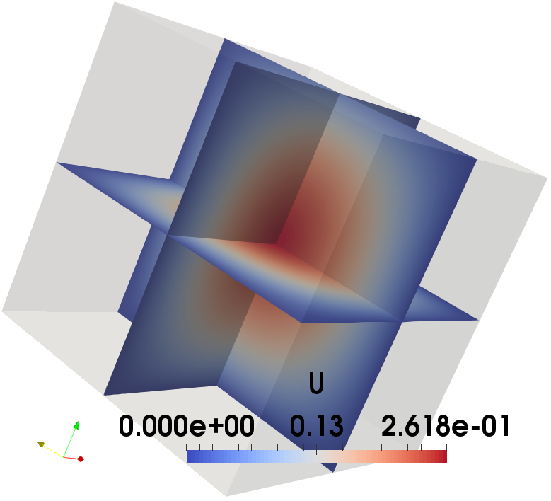
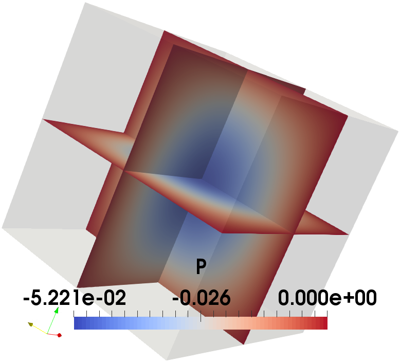
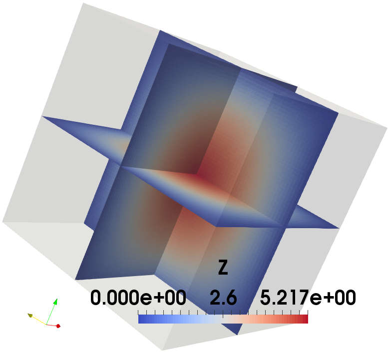
Figure 1: Example 1, numerical solutions of $u$, $p$, and $z$ for the linear model problem (from left to right).

The estimated order of convergence (eoc) is provided in Tables 1-3. From these results, we clearly see optimal convergence in $Y=L^{2}(0,T;H^{1}_{0}(\Omega))$ as predicted by Theorem 2. In addition, we observe a nearly optimal convergence rate in $L^{2}(Q)$. Finally, we see the second-order convergence rate of the objective functional.

Table 1: Example 1, estimated order of convergence (eoc) for $u_{h}$ and $p_{h}$ in $Y$ for the linear model problem.

#Dofs	$h$	$\|u-u_{h}\|_{Y}$	eoc	$\|p-p_{h}\|_{Y}$	eoc
$250$	$2^{-2}$	$2.218e-1$	$-$	$4.201e-2$	$-$
$1,458$	$2^{-3}$	$1.141e-1$	$0.959$	$2.235e-2$	$0.910$
$9,826$	$2^{-4}$	$5.677e-2$	$1.007$	$1.123e-2$	$0.993$
$71,874$	$2^{-5}$	$2.816e-2$	$1.012$	$5.588e-3$	$1.007$
$549,250$	$2^{-6}$	$1.400e-2$	$1.008$	$2.781e-3$	$1.006$
$2,146,689$	$2^{-7}$	$6.983e-3$	$1.004$	$1.387e-3$	$1.003$

Table 2: Example 1, estimated order of convergence (eoc) for $u_{h}$ and $p_{h}$ in $L^{2}(Q)$ for the linear model problem.

#Dofs	$h$	$\|u-u_{h}\|_{L^{2}(Q)}$	eoc	$\|p-p_{h}\|_{L^{2}(Q)}$	eoc
$250$	$2^{-2}$	$3.767e-2$	$-$	$4.146e-3$	$-$
$1,458$	$2^{-3}$	$1.156e-2$	$1.704$	$1.160e-3$	$1.837$
$9,826$	$2^{-4}$	$3.009e-3$	$1.942$	$2.981e-4$	$1.961$
$71,874$	$2^{-5}$	$7.595e-4$	$1.986$	$7.515e-5$	$1.988$
$549,250$	$2^{-6}$	$1.927e-4$	$1.979$	$1.950e-5$	$1.947$
$2,146,689$	$2^{-7}$	$4.948e-5$	$1.961$	$5.244e-6$	$1.894$

Table 3: Example 1, $J(u_{h},z_{h})$ and $|J(u_{h},z_{h})-J(u,z)|$ for the linear model problem, where $J(u,z)=9.53329e-2$.

#Dofs	$h$	$J(u_{h},z_{h})$	$|J(u_{h},z_{h})-J(u,z)|$	eoc
$250$	$2^{-2}$	$1.04613e-1$	$9.2801e-3$	$-$
$1,458$	$2^{-3}$	$9.80559e-2$	$2.7230e-3$	$1.769$
$9,826$	$2^{-4}$	$9.60214e-2$	$6.8850e-4$	$1.984$
$71,874$	$2^{-5}$	$9.55024e-2$	$1.6950e-4$	$2.022$
$549,250$	$2^{-6}$	$9.53748e-2$	$4.1900e-5$	$2.016$
$2,146,689$	$2^{-7}$	$9.53433e-2$	$1.0400e-5$	$2.010$

3.4.2 An example with discontinuous target (Example 2)

In the second example, the space-time domain $Q=(0,1)^{3}$ and the discontinuous target function

$$u_{d}(x,t)=\begin{cases}&1\quad\text{ if }\sqrt{(x_{1}-\frac{1}{2})^{2}+(x_{2}-\frac{1}{2})^{2}+(t-\frac{1}{2})^{2}}\leq\frac{1}{4},\\ &0\quad\textup{ else }\end{cases}$$

are considered. Further, we set homogeneous initial and boundary conditions for the state equation, and homogeneous terminal and boundary conditions for the adjoint equation. For the $L^{2}$-regularization parameter, we select $\varrho=10^{-6}$. Following the approach in [42], we have utilized a residual based error indicator to drive our mesh refinements in order to resolve the discrete optimality system. The space-time finite element solutions for the state and adjoint variables, as well as the time-dependent target are displayed in Fig. 2. The control is reconstructed by a postprocessing step using piecewise constant ansatz functions, which is demonstrated in the last column in Fig. 2. For a discussion and an error analysis of this postprocessing idea, we refer to [39] in the case of elliptic PDE control. The adaptive mesh is illustrated in Fig. 3 at the $20$th refining step, which contains $2,080,493$ grid points, i.e., the total number of degrees of freedom for the coupled state and adjoint equation is $4,160,986$.

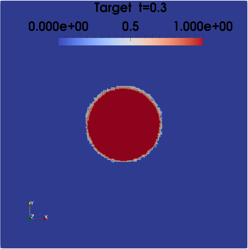
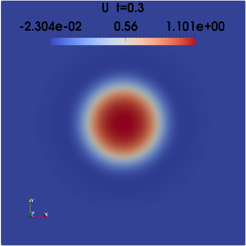
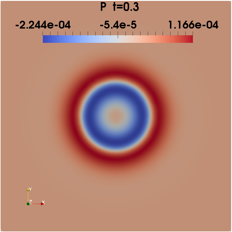
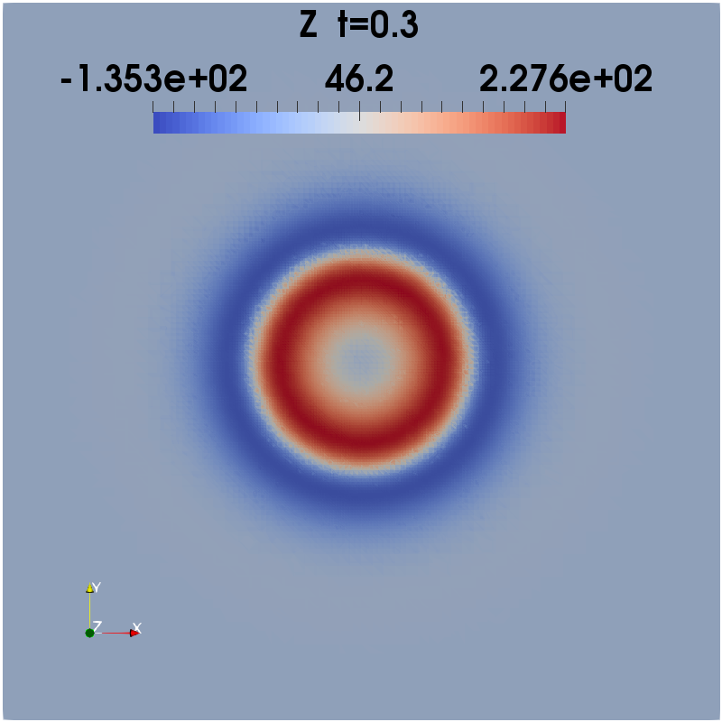
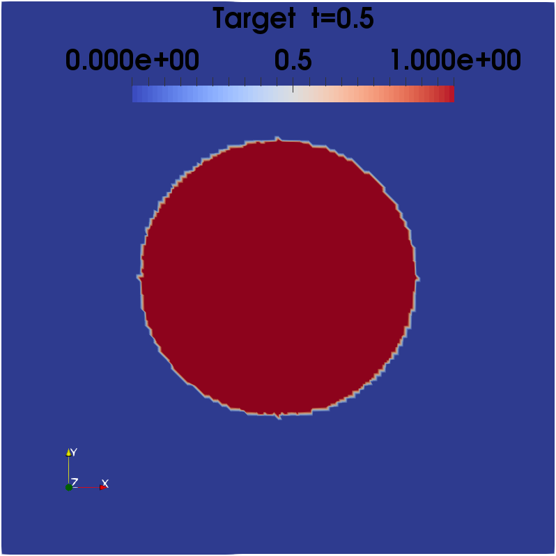
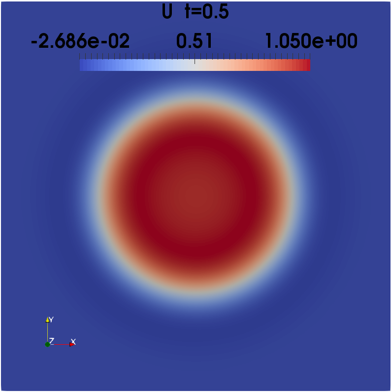
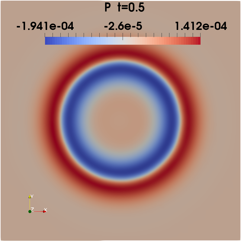
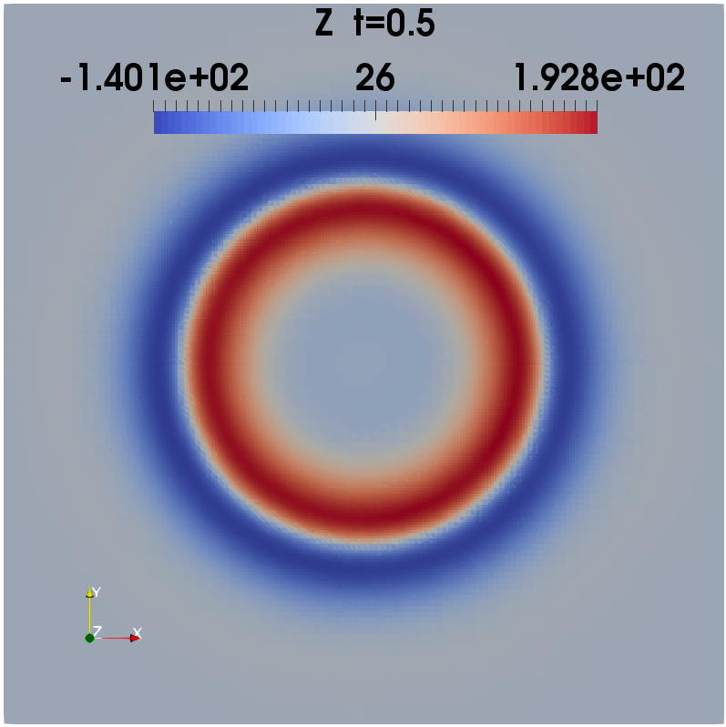
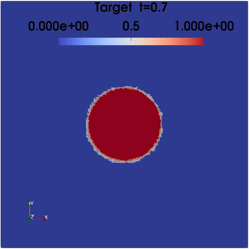
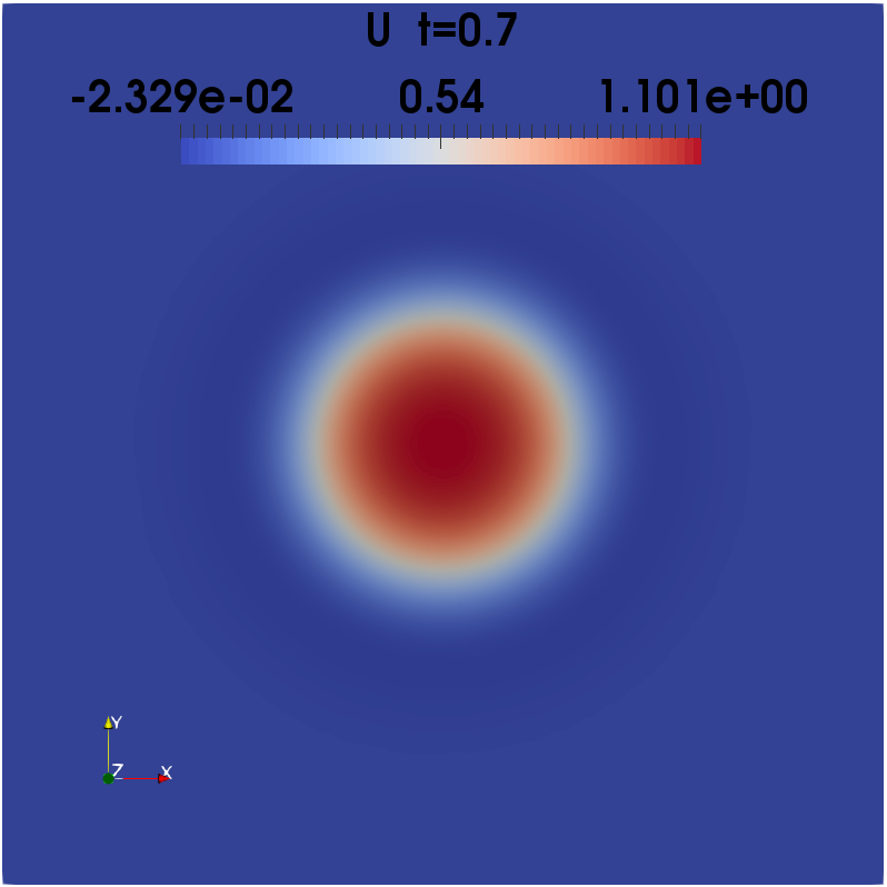
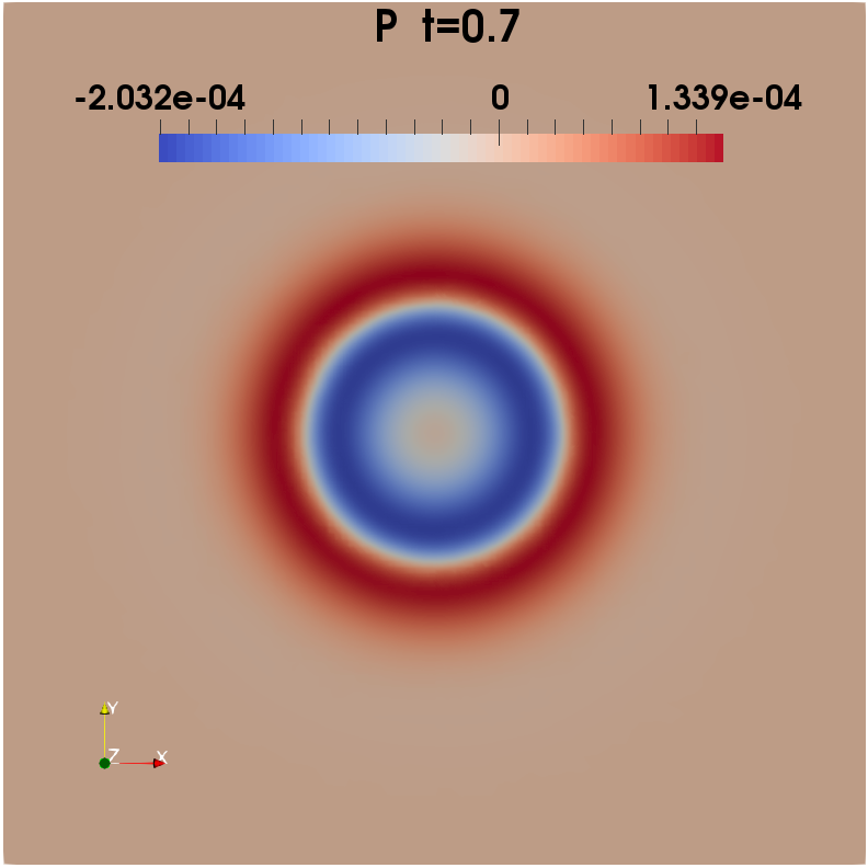
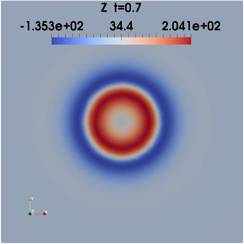
Figure 2: Example 2, numerical solutions of $u$, $p$, and $z$ for the linear model problem with a discontinuous target, at $t=0.3$, $0.5$, and $0.7$ (from top to bottom).

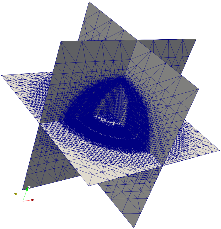
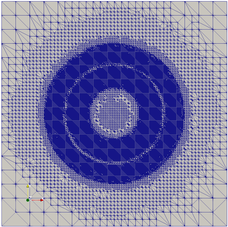
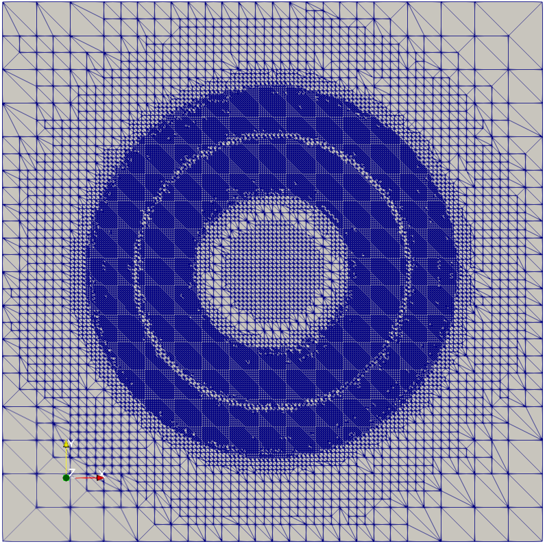
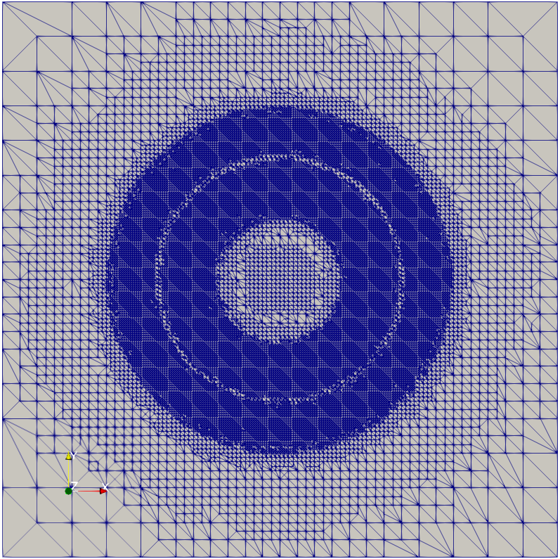
Figure 3: Example 2, adaptive mesh refinement at the $20$th step in space-time at $t=0.375$, $0.5$, and $0.625$ (from left to right), with a discontinuous target.

4 Control of a semilinear parabolic equation

4.1 The control problem

Here, we consider the following optimal control problem for a semilinear heat equation to minimize

$$J(u,z):=\frac{1}{2}\int_{Q}(u-u_{d})^{2}\,dx\,dt+\frac{\varrho}{2}\int_{Q}z^{2}\,dx\,dt$$ (24)

subject to

$$\partial_{t}u-\Delta_{x}u+R(u)=z\mbox{ in }Q,\quad\partial_{n}u=0\mbox{ in }\Sigma,\quad u=0\mbox{ on }\Sigma_{0}.$$ (25)

The control $z$ is taken from the space $L^{p}(Q)$ with $p>1+d/2$ to guarantee existence and uniqueness of a bounded solution $u$ to (25). We look for the solution $u$ of (25) in the space $Y\cap L^{\infty}(Q)$. Moreover, we here assume $u_{d}\in L^{p}(Q)$ to ensure later that the adjoint state belongs to $L^{\infty}(Q)$.

The function $R:\mathbb{R}\to\mathbb{R}$ is a $C^{2}$-function with locally Lipschitz second-order derivative, i.e., for all $M>0$, there is some $L(M)>0$ such that

$$|R^{\prime\prime}(v_{1})-R^{\prime\prime}(v_{2})|\leq L(M)\,|v_{1}-v_{2}|\quad\forall v_{i}\mbox{ with }|v_{i}|\leq M,i=1,2.$$

Moreover, we require the existence of some $c_{0}\in\mathbb{R}$ (possibly negative) such that

$$R^{\prime}(u)\geq c_{0}\quad\forall u\in\mathbb{R}.$$

An important particular case for the reaction term $R$ is

$$R(u)=(u-u_{1})(u-u_{2})(u-u_{3}),$$

where real numbers $u_{1}\leq u_{2}\leq u_{3}$ are given. Obviously, this function obeys the assumptions above. It is used for the Schlögl and FitzHugh-Nagumo equations. The following theorem on the solvability of (25) is known:

Theorem 3 ([14]).

Let $\Omega\subset{\mathbb{R}}^{d}$, $d\leq 3$, be a bounded Lipschitz domain and let $R$ satisfy the conditions stated above. Then for all controls $z\in L^{p}(Q)$ with $p>1+d/2$, the equation (25) has a unique solution $u\in Y\cap L^{\infty}(Q)$. The control-to-state mapping $G:z\mapsto u$ is of class $C^{2}$.

The optimal control problem (24)-(25) can be expressed in the reduced form

$$\min_{z\in L^{p}(Q)}f(z):=\frac{1}{2}\int_{Q}(G(z)-u_{d})^{2}\,dx\,dt+\frac{\varrho}{2}\int_{Q}z^{2}\,dx\,dt.$$

Compared with the quadratic optimal control problems of the former sections, several new difficulties occur.

Though we have $f(u)\to\infty$ if $\|z\|_{L^{2}(Q)}\to\infty$, the existence of an optimal control $\bar{z}$ cannot be proved by standard weak compactness techniques. It was recently shown by fairly deep arguments that at least one (globally) optimal control exists for the unconstrained case, cf. [13, 16]. This justifies to consider the optimal control problem without control constraints.

Moreover, even though the functional $J$ is convex, the reduced functional $f$ is not in general convex, because $G$ is nonlinear. Therefore, the optimality system is not sufficient for (local or global) optimality of its solution. We might also have different global or local solutions of the optimal control problem. They are even not guaranteed to be locally unique. To overcome these difficulties, we assume that a given reference solution of the optimality system satisfies a second-order sufficient optimality condition.

Finally, we should mention that the mapping $G$ is not in general differentiable or twice differentiable in the Hilbert space $L^{2}(Q)$.

To allow for a Hilbert space setting as in the previous sections, we will proceed as follows: In the infinite-dimensional setting, we will apply a Newton method (sequential quadratic programming (SQP) method) that solves the problem by a sequence of quadratic optimal control problems that are posed in Hilbert space. These are solved by the methods of the former sections. For convergence of this method, the second-order sufficient optimality condition is needed again.

4.2 The Lagrange-Newton-SQP method

Let us define the Lagrangian $\mathcal{L}:(Y\cap L^{\infty}(Q))^{2}\times L^{p}(Q)\to\mathbb{R}$, $p>1+d/2$, by

$$\mathcal{L}(u,p,z)=J(u,z)-\int_{Q}\Big{(}\partial_{t}u\,p+\nabla u\cdot\nabla p+R(u)\,p-z\,p\Big{)}\,dx\,dt.$$

Then the SQP method proceeds as follows: An arbitrary triplet $(u_{0},p_{0},z_{0})\in(Y\cap L^{\infty}(Q))^{2}\times L^{p}(Q)$ is taken as initial iterate. For a given iterate $(u_{n},p_{n},z_{n})$ the following quadratic optimal control problem ($QP_{n}$) is considered:

$$\left.\begin{array}[]{l}\min J^{\prime}(u_{n},z_{n})(u-u_{n},z-z_{n})+\displaystyle\frac{1}{2}\mathcal{L}_{u,z}^{\prime\prime}(u_{n},p_{n},z_{n})(u-u_{n},z-z_{n})^{2}\\[8.61108pt] \qquad\mbox{subject to the linearized equation}\\[8.61108pt] \begin{array}[]{rcll}\partial_{t}u-\Delta_{x}u+R(u_{n})+R^{\prime}(u_{n})(u-u_{n})&=&z&\mbox{in}\;Q,\\[2.84526pt] \partial_{n}u&=&0&\mbox{on}\;\Sigma,\\[2.84526pt] u&=&0&\mbox{on}\;\Sigma_{0}.\end{array}\end{array}\right\}$$

The next iterate $z_{n+1}$ is the optimal control of ($QP_{n}$), provided that it exists, $u_{n+1}$ is the associated optimal state and $p_{n+1}$ is the associated adjoint state.

The numerical treatment of ($QP_{n}$) requires the solution of the optimality system

$$\left.\begin{array}[]{lcl}\partial_{t}u-\Delta_{x}u+R(u_{n})+R^{\prime}(u_{n})(u-u_{n})+\displaystyle\frac{1}{\varrho}\,p&=&0,\;u(0)=u_{0},\\[8.61108pt] -\partial_{t}p-\Delta_{x}p+R^{\prime}(u_{n})p+p_{n}R^{\prime\prime}(u_{n})(u-u_{n})&=&u_{n}-u_{d},\;p(T)=0\end{array}\right\}$$

subject to homogeneous Neumann conditions. Then we have $u_{n+1}=u$ and $p_{n+1}=p$; the new control iterate is $z_{n+1}=-p_{n+1}/\varrho.$ This iteration method is called Lagrange-Newton method, because it comes from linearizing the whole optimality system. In contrast to this, the SQP method would not linearize the state equation. We refer for a general exposition to [2, 3], for the convergence analysis for semilinear parabolic equations in an $L^{\infty}$-setting to [45, 46] and the discussion in a Hilbert space setting to [25].

To make all iterates well defined, we will invoke a second-order sufficient optimality condition.

4.3 Second-order sufficient optimality condition and convergence of the Lagrange-Newton method

Let $(\bar{u},\bar{p},\bar{z})$ be a fixed triplet that satisfies the optimality system for the optimal control problem (24)-(25). We say that the triplet fulfils the second-order sufficient optimality condition, if it enjoys the following property of positive definiteness: A number $\sigma>0$ exists, such that

$$\mathcal{L}^{\prime\prime}_{u,z}(\bar{u},\bar{p},\bar{z})(u,z)^{2}\geq\sigma\,\|z\|_{L^{2}(Q)}^{2}$$ (25)

holds for all pairs $(u,z)$ that obey the linearized equation

$$\partial_{t}u-\Delta_{x}u+R^{\prime}(\bar{u})u=z\;\mbox{in}\;Q,\quad\partial_{n}u=0\;\mbox{on}\;\Sigma,\quad u=0\;\mbox{on}\;\Sigma_{0}.$$

It is known that this condition is sufficient for the local optimality of $\bar{z}$ in the sense of $L^{2}(Q)$, [15]. Moreover, $\bar{z}$ is unique in a certain $L^{2}(\Omega)$-neighborhood. It is not in general possible to verify this condition by numerical methods. As usual, it is just a theoretical basis for the analysis.

In the case of the optimal control problem (24)-(25), the derivative $\mathcal{L}^{\prime\prime}$ has the form

$$\mathcal{L}^{\prime\prime}_{u,z}(\bar{u},\bar{p},\bar{z})(u,z)^{2}=\|u\|_{L^{2}(Q)}^{2}+\varrho\,\|z\|_{L^{2}(Q)}^{2}-\int_{Q}\bar{p}\,R^{\prime\prime}(\bar{u})\,u^{2}\,dx\,dt.$$

Therefore, the second-order sufficient optimality condition is satisfied in particular, if

$$1-\bar{p}(x,t)\,R^{\prime\prime}(\bar{u}(x,t))\geq\sigma\quad\mbox{ for a.a. }(x,t)\in Q.$$

For instance, this holds, if $\bar{p}$ is small, i.e., $\bar{u}$ is close to $u_{d}$. The convergence theorem below is based on the second-order sufficient condition. Since it needs box constraints on the control to ensure that all iterates belong to a bounded set of $L^{\infty}(Q)$, we invoke the following result:

Lemma 4.

There is at least one optimal control of problem (24)-(25) that belongs to $L^{\infty}(Q)$.

Proof.

We rely on Theorem 2.4 of [16] that guarantees the existence of at least one optimal control $\bar{u}$ of (24)-(25) that is bounded in $L^{\infty}(0,T;L^{2}(\Omega))$. Therefore, the search for a control can be restricted to the set $\{u\in L^{\infty}(0,T;L^{2}(\Omega)):\|u\|_{L^{\infty}(0,T;L^{2}(\Omega))}\leq R\}$, where $R=\|\bar{u}\|_{L^{\infty}(0,T;L^{2}(\Omega))}$. Thanks to the existence and regularity Theorem 2.1 of [16], all associated states are bounded in $L^{\infty}(Q)$. The right-hand side of the associated adjoint equation is $\bar{u}-u_{d}\in L^{p}(Q)$, since we assumed $u_{d}\in L^{p}(Q)$. Therefore, the adjoint state $\bar{p}$ is also a function of $L^{\infty}(Q)$. This property transfers to $\bar{u}$ by the gradient equation $\bar{u}=-\bar{p}/\varrho$, hence the existence of an optimal control in $L^{\infty}(Q)$ is proved. ∎

The following result is known for the convergence of the Lagrange-Newton-SQP method for problems of the type (24)-(25) with additional box constraints

$$a\leq u(x,t)\leq b\quad\mbox{for a.a. }(x,t)\in Q,$$ (26)

where $-\infty<a<b<\infty$:

Theorem 4 (Convergence of the Lagrange-Newton method).

Let $(\bar{u},\bar{p},\bar{z})$ be a triplet that satisfies the optimality system for the optimal control problem (24)-(25) with additional box constraints (26). Assume that this triplet satisfies the second-order sufficient condition (25).

Then the Lagrange-Newton method converges locally and quadratic to $(\bar{u},\bar{p},\bar{z})$. This means the following: There exist $r>0,\,C>0$ such that, if the initial iterate $(u_{0},p_{0},z_{0})\in(Y\cap L^{\infty}(Q))^{2}\times L^{\infty}(Q)$ satisfies

$$\|(u_{0},p_{0},z_{0})-(\bar{u},\bar{p},\bar{z})\|_{L^{\infty}(Q)^{3}}\leq r,$$

then the system ($OS_{n}$) is uniquely solvable for all $n\geq 0$. The iterates fulfill

$$\|(u_{n},p_{n},z_{n})-(\bar{u},\bar{p},\bar{z})\|_{L^{\infty}(Q)^{3}}\leq r,\quad\forall n\geq 1,$$

and

$$\|(u_{n+1},p_{n+1},z_{n+1})-(\bar{u},\bar{p},\bar{z})\|_{L^{\infty}(Q)^{3}}\leq C\,\|(u_{n},p_{n},z_{n})-(\bar{u},\bar{p},\bar{z})\|_{L^{\infty}(Q)^{3}}^{2}$$

for all $n\geq 0$.

The proof is a bit delicate, because the $L^{2}(Q)$-norm appears in the second-order sufficient condition, while the differentiability of $\mathcal{L}$ is considered in $L^{\infty}(Q)$. This is the so-called two-norm discrepancy. For a proof with additional control constraints $a\leq z\leq b$, we refer to [45]. For problems, where the two-norm-discrepancy does not appear, a convergence analysis for the Newton method in the unconstrained method is given in [17] and, in the context of optimal control, in [25].

The Lagrange-Newton-SQP method differs from the Lagrange-Newton method by adding the box constraints (26) to the subproblems (QP_n) and the associated projection formula to the optimality system (QP_n). In our implementation, we formally added box constraints with $a=-10^{6}$, $b=10^{6}$, justified by Lemma 4. These bounds became never active. Hence, the Lagrange-Newton-SQP method was equivalent to the Lagrange-Newton method described in the last subsection.

4.4 Numerical experiments

For the nonlinear first order necessary optimality system, when considering a nonlinear reaction term in the state equation or in the presence of box constraints on the control, we apply a (semismooth) Newton method in the outer iteration. Usually, we need about $2-8$ iterations to reach a precision of $10^{-8}$ of the relative residual error. Inside each Newton iteration, we apply the same algebraic multigrid preconditioned GMRES solver as used for the linear system. However, the performance study and the development of robust and efficient solvers are beyond the scope of this work; we will investigate them somewhere else.

4.4.1 Unconstrained control with explicitly known optimal solution (Example 3)

Following the approach provided in [46], we construct an exact solution for the following modified optimal control problem of a semilinear parabolic equation:

$$\min J(u,z):=\frac{1}{2}\int_{Q}(u-u_{d})^{2}\,dx\,dt+\frac{\varrho}{2}\int_{Q}z^{2}\,dx\,dt$$

subject to

$$\partial_{t}u-\Delta_{x}u+R(u)=z+e_{u}\;\mbox{in }Q,\quad u=0\;\mbox{on }\Sigma,\quad u=0\;\mbox{on }\Sigma_{0},$$

where the function $e_{u}$ is defined such that a desired pair $u$, $z$ is optimal. The first order necessary optimality system for this semilinear model problem reads as follows (see [46]): It is composed of the state equation

$$\partial_{t}u-\Delta_{x}u+R(u)+\frac{1}{\varrho}p=e_{u}\textup{ in }Q,\quad u=0\textup{ on }\Sigma,\quad u=0\textup{ on }\Sigma_{0},$$ (27)

and the adjoint equation

$$-\partial_{t}p-\Delta_{x}p+R^{\prime}(u)p=u-u_{d}\textup{ in }Q,\quad p=0\textup{ on }\Sigma,\quad p=0\textup{ on }\Sigma_{T}.$$ (28)

The desired solutions of the optimality system are given by

$$u(x,t)=\sin(\pi x_{1})\sin(\pi x_{2})\left(at^{2}+bt\right),$$

$$p(x,t)=-\varrho\sin(\pi x_{1})\sin(\pi x_{2})\left(2\pi^{2}at^{2}+(2\pi^{2}b+2a)t+b\right),$$

$$z(x,t)=\sin(\pi x_{1})\sin(\pi x_{2})\left(2\pi^{2}at^{2}+(2\pi^{2}b+2a)t+b\right),$$

$$R(u)=u(u-0.25)(u+1),$$

where $a=-\frac{2\pi^{2}+1}{2\pi^{2}+2}$, $b=1$, and $\varrho=10^{-4}$. It is easy to see that the state obeys homogeneous initial and boundary conditions, and the adjoint state satisfies homogeneous terminal and boundary conditions; see the illustration in Fig. 4. The functions $e_{u}$ and $u_{d}$ are computed by inserting the above solutions to the system (27) and (28).

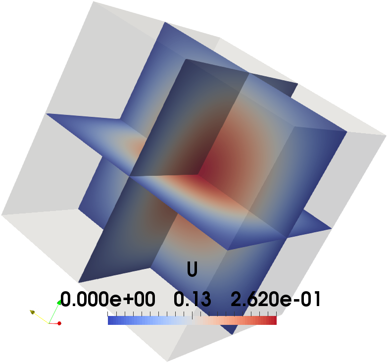
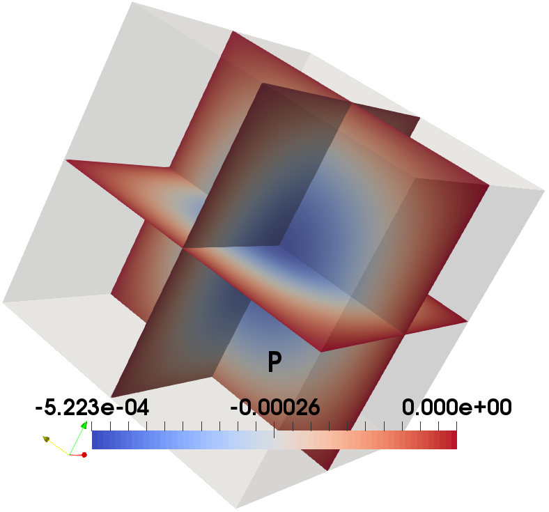
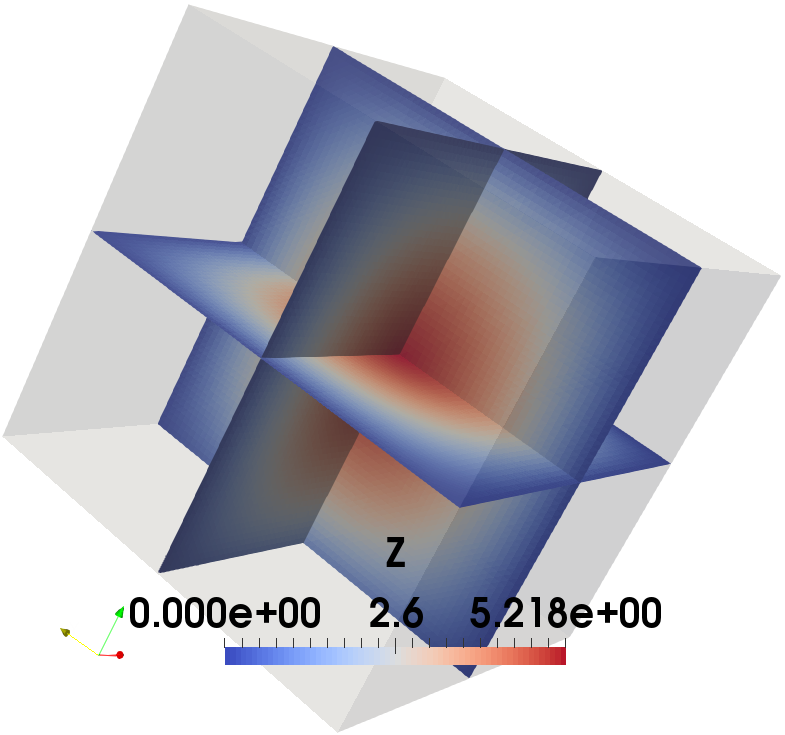
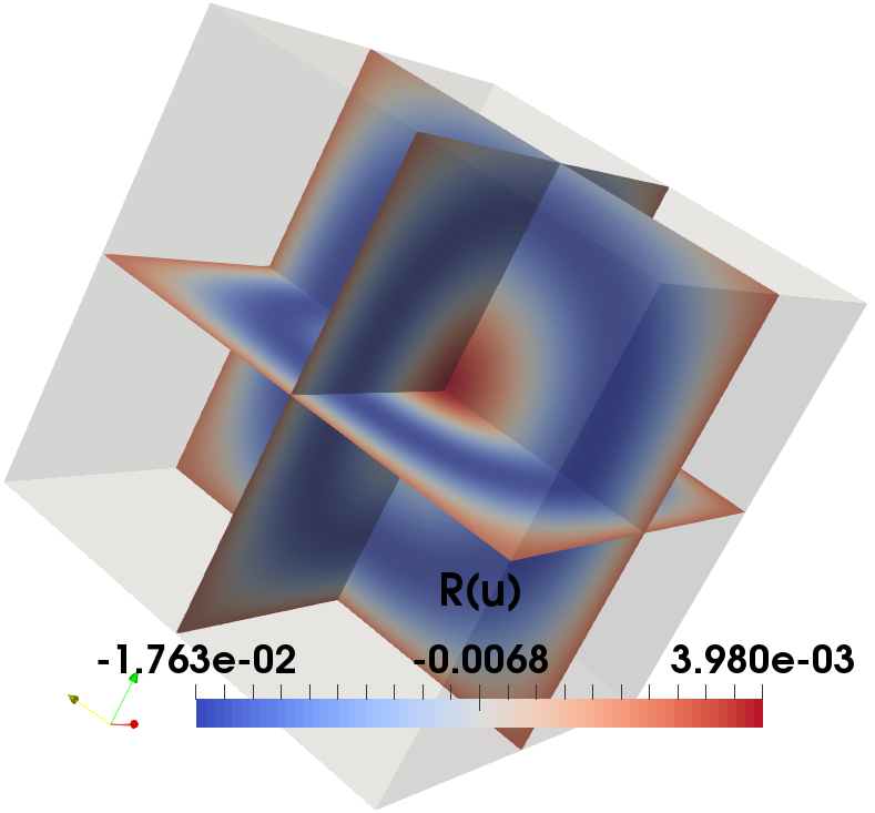
Figure 4: Example 3, numerical solutions of $u$, $p$, and $z$, and $R(u)$ for the semilinear model problem without control constraint.

The estimated order of convergence is given in Tables 4-6. As we expect, we observe optimal convergence rates in $Y=L^{2}(0,T;H^{1}_{0}(\Omega))$. However, the convergence rate is not that good as expected in $L^{2}(Q)$ for this particular example. This requires further investigation. Moreover, we see almost second-order convergence for the objective functional.

Table 4: Example 3, estimated order of convergence (eoc) of $u_{h},p_{h}$ in $Y$ for the semilinear model problem without control constraint.

#Dofs	$h$	$\|u-u_{h}\|_{Y}$	eoc	$\|p-p_{h}\|_{Y}$	eoc
$250$	$2^{-2}$	$2.344e-1$	$-$	$8.136e-4$	$-$
$1,458$	$2^{-3}$	$1.159e-1$	$1.017$	$2.795e-4$	$1.541$
$9,826$	$2^{-4}$	$5.690e-2$	$1.026$	$1.193e-4$	$1.228$
$71,874$	$2^{-5}$	$2.815e-2$	$1.015$	$5.691e-5$	$1.068$
$549,250$	$2^{-6}$	$1.400e-2$	$1.008$	$2.801e-5$	$1.023$
$2,146,689$	$2^{-7}$	$6.982e-3$	$1.003$	$1.394e-5$	$1.007$

Table 5: Example 3, estimated order of convergence of $u_{h},p_{h}$ in $L^{2}(Q)$ for the semilinear model problem without control constraint.

#Dofs	$h$	$\|u-u_{h}\|_{L^{2}(Q)}$	eoc	$\|p-p_{h}\|_{L^{2}(Q)}$	eoc
$250$	$2^{-2}$	$1.315e-2$	$-$	$9.435e-5$	$-$
$1,458$	$2^{-3}$	$3.692e-3$	$1.833$	$2.104e-5$	$2.165$
$9,826$	$2^{-4}$	$1.008e-3$	$1.873$	$4.770e-6$	$2.141$
$71,874$	$2^{-5}$	$2.621e-4$	$1.943$	$1.213e-6$	$1.976$
$549,250$	$2^{-6}$	$7.218e-5$	$1.861$	$3.542e-7$	$1.775$
$2,146,689$	$2^{-7}$	$3.180e-5$	$1.183$	$1.417e-7$	$1.321$

Table 6: Example 3, $J(u_{h},z_{h})$ and $|J(u_{h},z_{h})-J(u,z)|$ for the semilinear model problem without control constraint, where $J(u,z)=1.98767e-4$.

#Dofs	$h$	$J(u_{h},z_{h})$	$|J(u_{h},z_{h})-J(u,z)|$	eoc
$250$	$2^{-2}$	$4.60861e-4$	$2.6209e-4$	$-$
$1,458$	$2^{-3}$	$2.37900e-4$	$3.9133e-5$	$2.744$
$9,826$	$2^{-4}$	$2.06470e-4$	$7.7030e-6$	$2.345$
$71,874$	$2^{-5}$	$2.00532e-4$	$1.7650e-6$	$2.126$
$549,250$	$2^{-6}$	$1.99206e-4$	$4.3900e-7$	$2.007$
$2,146,689$	$2^{-7}$	$1.98887e-4$	$1.2000e-7$	$1.871$

4.4.2 Box constrained control with explicitly known optimal solution (Example 4)

In this example, we minimize

$$J(u,z):=\frac{1}{2}\int_{Q}(u-u_{d})^{2}\,dx\,dt+\frac{\varrho}{2}\int_{Q}z^{2}\,dx\,dt+\int_{Q}e_{z}\,z\,dx\,dt$$

subject to

$$\partial_{t}u-\Delta_{x}u+R(u)=z+e_{u}\textup{ in }Q,\quad u=0\textup{ on }\Sigma,\quad u=0\textup{ on }\Sigma_{0},$$

and

$$a\leq z(x,t)\leq b\quad\textup{ for a.a. }(x,t)\in Q.$$

For this optimal control problem, we compute the functions $e_{u}$ and $e_{z}$ such that the desired solutions $u$, $p$ and $z$ satisfy the first order necessary optimality conditions. This system consists of the state equation

$$\partial_{t}u-\Delta_{x}u+R(u)=z+e_{u}\text{ in }Q,\quad u=0\text{ on }\Sigma,\quad u=0\text{ on }\Sigma_{0},$$

the adjoint equation

$$-\partial_{t}p-\Delta_{x}p+R^{\prime}(u)p=u-u_{d}\text{ in }Q,\quad p=0\text{ on }\Sigma,\quad p=0\text{ on }\Sigma_{T},$$

and the gradient equation

$$z={\mathbf{P}}_{[a,b]}\left(-\frac{1}{\varrho}\left(p+e_{z}\right)\right)\text{ in }Q.$$

The projection formula is equivalent to the variational inequality

$$\int_{Q}(p+\varrho z+e_{z})(\hat{z}-z)\,dx\,dt\geq 0\textup{ for all }\hat{z}\in[a,b],$$ (29)

for more details, see [46].

We now prescribe the solutions of the optimality system as follows:

$$u(x,t)=\sin(\pi x_{1})\sin(\pi x_{2})\left(ct^{2}+dt\right),$$

$$p(x,t)=-\varrho\sin(\pi x_{1})\sin(\pi x_{2})\left(2\pi^{2}ct^{2}+(2\pi^{2}d+2c)t+d\right),$$

$$z(x_{1},x_{2},t)=\begin{cases}-1&\textup{ if }0\leq x_{2}\leq-x_{1}+1/2\textup{ and }0\leq x_{1}\leq 1/2,\\ 1&\textup{ if }-x_{1}+3/2\leq x_{2}\leq 1\textup{ and }1/2\leq x_{1}\leq 1,\\ 2x_{1}+2x_{2}-2&\textup{ else },\\ \end{cases}$$

where $c=-\frac{2\pi^{2}+1}{2\pi^{2}+2}$ and $d=1$. As nonlinearity, we fix $R(u)=u(u-0.25)(u+1)$. For the constraints, we use the bounds $a=-1$ and $b=1$, and we set $\varrho=0.001$ as regularization parameter. The constructed solutions $u$ and $p$ fulfill the initial/terminal and boundary conditions for the state and adjoint; see the numerical solutions in Fig. 5 for an illustration.

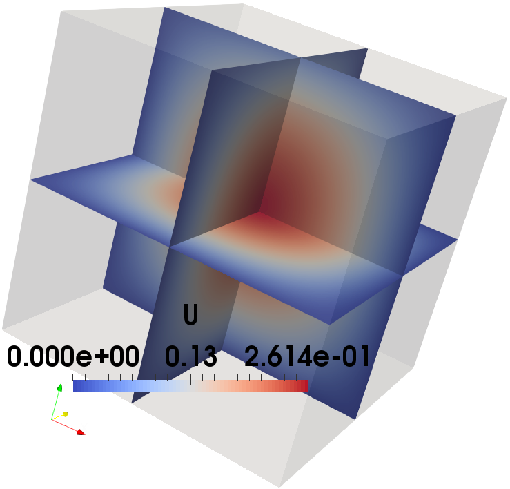
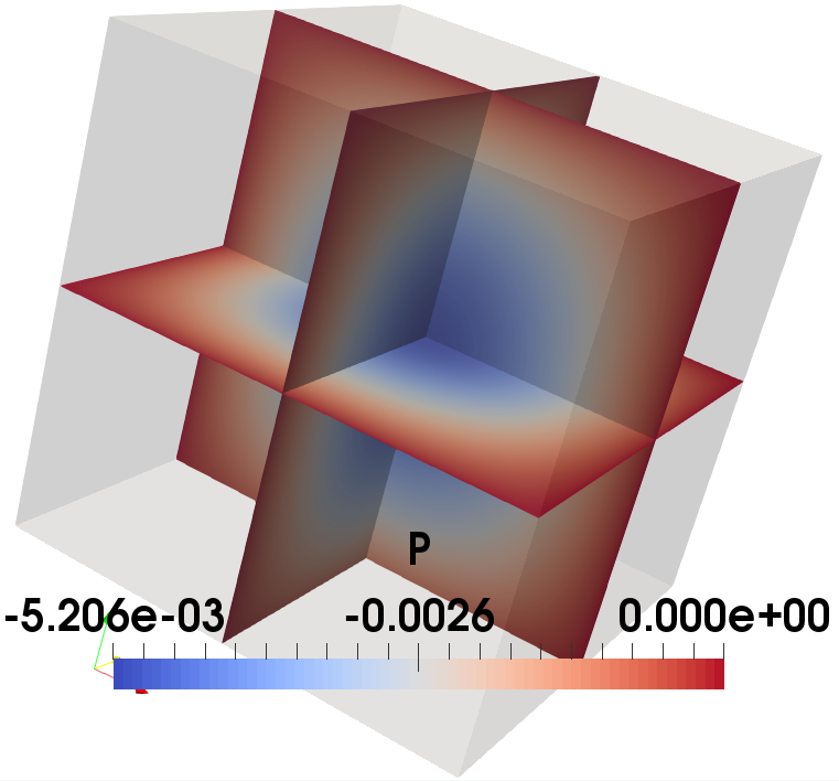
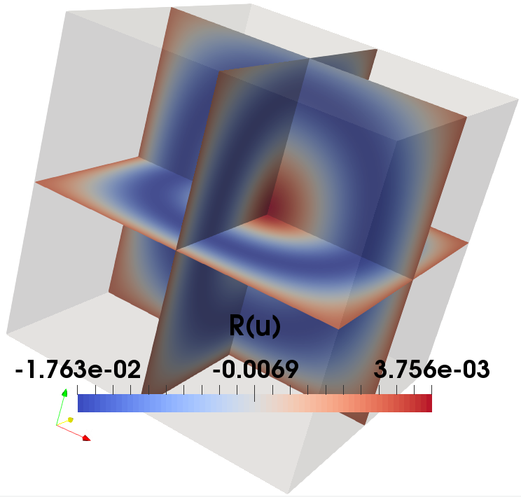
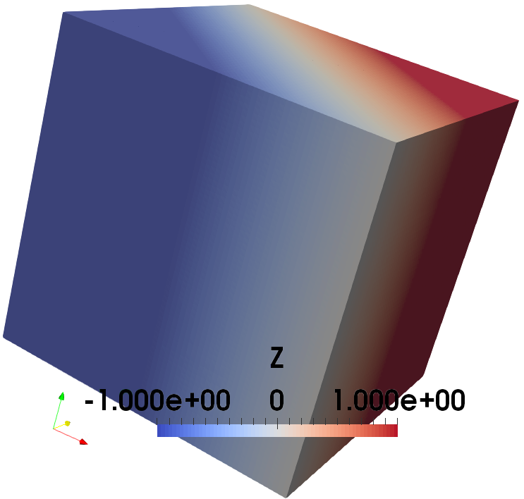
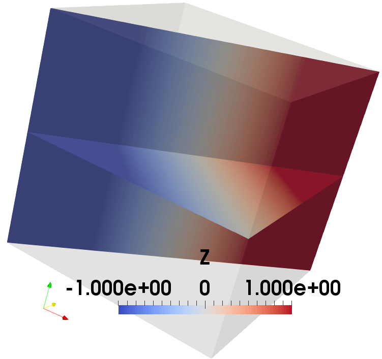
Figure 5: Example 4, numerical solutions of $u$, $p$, and $z$, and $R(u)$ for the semilinear model problem with box constraint on control.

Inserting the exact solutions prescribed above in the primal and adjoint equations, respectively, the unknown functions $e_{u}$ and $u_{d}$ are obtained. Along with the defined active and inactive sets

$${\mathcal{A}}_{a}:=\{(x,t)\in Q:-\varrho^{-1}(p+e_{z})<a\},$$ (30)

$${\mathcal{A}}_{b}:=\{(x,t)\in Q:-\varrho^{-1}(p+e_{z})>b\},$$

$${\mathcal{I}}:=Q\backslash\{{\mathcal{A}}_{a}\cup{\mathcal{A}}_{b}\},$$

using the variational inequality (29), we can construct the remaining unknown function $e_{z}$ as follows:

$$e_{z}=\begin{cases}{(p+\varrho a)_{-}}\textup{ on }{\mathcal{A}}_{a},\\ -(p+\varrho z)\textup{ on }{\mathcal{I}},\\ {-(p+\varrho b)_{+}}\textup{ on }{\mathcal{A}}_{b}.\end{cases}$$ (31)

Now, starting from the variational inequality (29), using a piecewise constant ansatz for the control, we arrive at the elementwise projection formula

$$z_{\ell}={\mathbf{P}}_{[a,b]}\left(-\frac{1}{\varrho|\tau_{\ell}|}\int_{\tau_{\ell}}(p_{h}+e_{z})\,dx\,dt\right),\quad\forall\tau_{\ell}\in{\mathcal{T}}_{h}(Q).$$ (32)

Inserting this formula in the discrete state equation, we obtain a coupled nonlinear first order necessary optimality system for the state and adjoint variables. This discrete nonlinear system is solved by the semismooth Newton method. After having computed $p_{h}$, in a final postprocessing step, we use the projection formula (32) to compute the optimal control as a piecewise linear and continuous function.

The estimated order of convergence in $Y=L^{2}(0,T;H^{1}_{0}(\Omega))$ is displayed in Table 7. We clearly observe an optimal convergence rate. For this example, we do not have optimal convergence in $L^{2}(Q)$; see Table 8. However, we see a second-order convergence rate for the objective functional; cf. Table 9.

Table 7: Example 4, estimated order of convergence (eoc) of $u_{h},p_{h}$ in $Y$ for the semilinear model problem with box constraints.

#Dofs	$h$	$\|u-u_{h}\|_{Y}$	eoc	$\|p-p_{h}\|_{Y}$	eoc
$250$	$2^{-2}$	$2.121e-1$	$-$	$5.272e-3$	$-$
$1,458$	$2^{-3}$	$1.126e-1$	$0.913$	$2.396e-3$	$1.138$
$9,826$	$2^{-4}$	$5.653e-2$	$0.995$	$1.142e-3$	$1.069$
$71,874$	$2^{-5}$	$2.817e-2$	$1.008$	$5.608e-4$	$1.026$
$549,250$	$2^{-6}$	$1.401e-2$	$1.005$	$2.790e-4$	$1.007$
$2,146,689$	$2^{-7}$	$7.017e-3$	$0.997$	$1.407e-4$	$0.988$

Table 8: Example 4, estimated order of convergence (eoc) of $u_{h},p_{h},z_{h}$ in $L^{2}(Q)$ for the semilinear model problem with box constraints ($\|\cdot\|=\|\cdot\|_{L^{2}(Q)}$).

#Dofs	$h$	$\|u-u_{h}\|$	eoc	$\|p-p_{h}\|$	eoc	$\|z-z_{h}\|$	eoc
$250$	$2^{-2}$	$2.133e-2$	$-$	$3.811e-4$	$-$	$3.072e-1$	$-$
$1,458$	$2^{-3}$	$5.873e-3$	$1.861$	$1.018e-4$	$1.905$	$9.984e-2$	$1.622$
$9,826$	$2^{-4}$	$1.566e-3$	$1.907$	$2.489e-5$	$2.032$	$3.251e-2$	$1.619$
$71,874$	$2^{-5}$	$4.733e-4$	$1.727$	$6.355e-6$	$1.970$	$1.379e-2$	$1.237$
$549,250$	$2^{-6}$	$2.224e-4$	$1.089$	$3.731e-6$	$0.768$	$7.435e-3$	$0.891$
$2,146,689$	$2^{-7}$	$1.741e-4$	$0.353$	$3.793e-6$	$-0.024$	$5.016e-3$	$0.568$

Table 9: Example 4, $J(u_{h},z_{h})$ and $|J(u_{h},z_{h})-J(u,z)|$ for the semilinear model problem with box constraint on control, where $J(u,z)=5.1743e-4$.

#Dofs	$h$	$J(u_{h},z_{h})$	$|J(u_{h},z_{h})-J(u,z)|$	eoc
$250$	$2^{-2}$	$1.8162e-3$	$1.299e-3$	$-$
$1,458$	$2^{-3}$	$8.1878e-4$	$3.014e-4$	$2.108$
$9,826$	$2^{-4}$	$5.8804e-4$	$7.061e-5$	$2.094$
$71,874$	$2^{-5}$	$5.3448e-4$	$1.705e-5$	$2.050$
$549,250$	$2^{-6}$	$5.2161e-4$	$4.180e-6$	$2.028$
$2,146,689$	$2^{-7}$	$5.1846e-4$	$1.030e-6$	$2.021$

4.4.3 Example with a turning wave (Example 5)

As final example, we consider the following optimal control problem:

$$\min{\mathcal{J}}(u,z):=\frac{1}{2}\int_{Q}(u-u_{d})^{2}\,dx\,dt+\frac{\varrho}{2}\int_{Q}z^{2}\,dx\,dt$$

subject to the state equation

$$\partial_{t}u-\Delta_{x}u+R(u)=z\text{ in }Q,\quad\partial_{n}u=0\text{ on }\Sigma,\quad u=u_{0}\text{ on }\Sigma_{0},$$

and

$$a\leq z(x,t)\leq b\quad\text{ for a.a. }(x,t)\in Q.$$

This simplified model problem is an adapted version of that one provided in [14], here without $L^{1}$-regularization. The first-order necessary optimality system for this model problem reads as follows: In addition to the above state equation, the adjoint equation is

$$-\partial_{t}p-\Delta_{x}p+R^{\prime}(u)p=u-u_{d}\text{ in }Q,\quad\partial_{n}p=0\text{ on }\Sigma,\quad p=0\text{ on }\Sigma_{T},$$

and the gradient equation reads

$$z={\mathbf{P}}_{[a,b]}\left(-\frac{1}{\varrho}p\right)\text{ in }Q.$$

As for the turning wave example constructed in [14], we define the nonlinear reaction term $R(u)=u(u-0.25)(u+1)$, the initial condition

$$u_{0}=\left(1+\exp\left(\frac{\frac{70}{3}-70x_{1}}{\sqrt{2}}\right)\right)^{-1}+\left(1+\exp\left(\frac{70x_{1}-\frac{140}{3}}{\sqrt{2}}\right)\right)^{-1}-1\textup{ on }\Sigma_{0}$$

for the state, and the target

$${u}_{d}=\left(1.0+\exp\left(\frac{\cos(g(t))\left(\frac{70}{3}-70x_{1}\right)+\sin(g(t))\left(\frac{70}{3}-70x_{2}\right)}{\sqrt{2}}\right)\right)^{-1}$$

$$\quad+\left(1.0+\exp\left(\frac{\cos(g(t))\left(70x_{1}-\frac{140}{3}\right)+\sin(g(t))\left(70x_{2}-\frac{140}{3}\right)}{\sqrt{2}}\right)\right)^{-1}-1$$

in $Q$, where $g(t)=\frac{2\pi}{3}\min\left\{\frac{3}{4},t\right\}$. We should mention that the target defined in [14] contained a typo; this is corrected here. The wave front turns $90$ degrees from time $t=0$ to $t=0.75$ and remains fixed after $t=0.75$; see the target at $t=0$, $0.25$, $0.5$, and $0.75$ illustrated in Fig. 6.

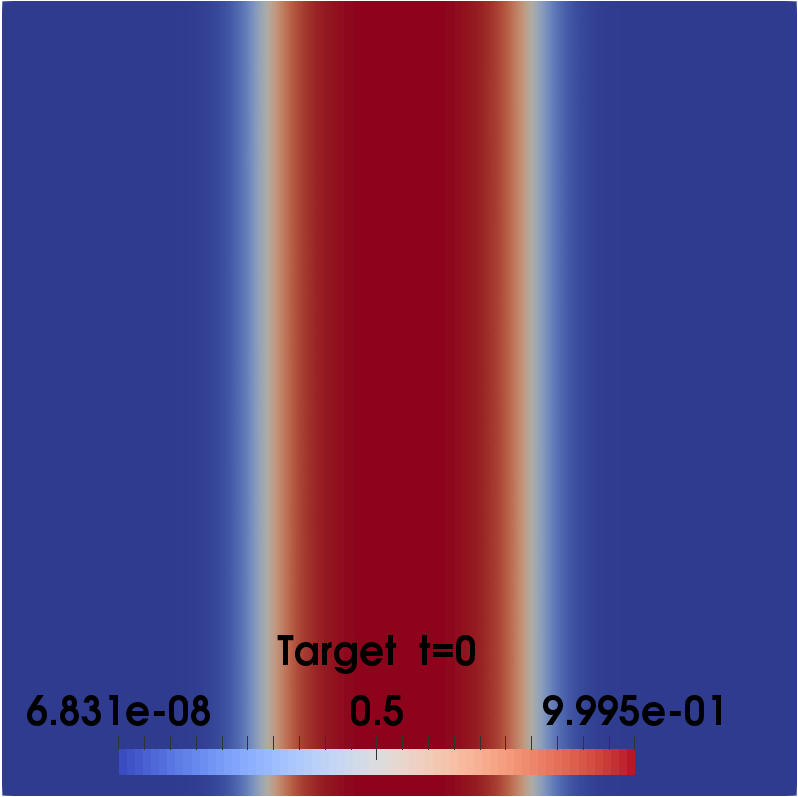
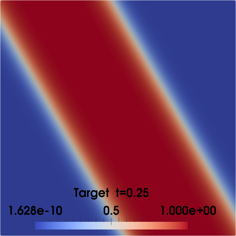
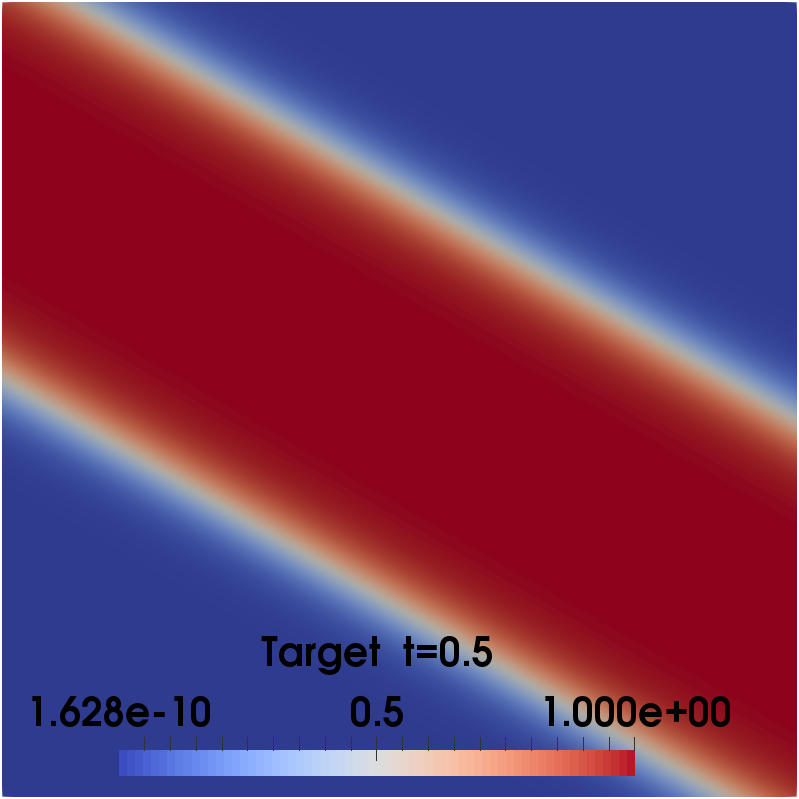
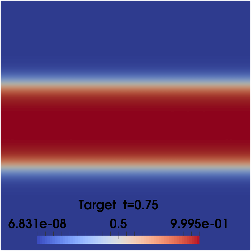
Figure 6: Example 5, plots of the target at time $t=0,\;0.25,\;\;0.5,\;0.75$ for the turning wave example.

As parameters, we use $\varrho=10^{-6}$, $a=-10^{+6}$, and $b=10^{+6}$ in the unconstrained case, while $a=-10^{+2}$ and $b=10^{+2}$ are set in the constrained case. We then follow the approach of the previous section to solve the coupled nonlinear first order optimality system by the semismooth Newton method. The numerical solutions for state, adjoint state, and control in the space-time domain are visualized in Fig. 7.

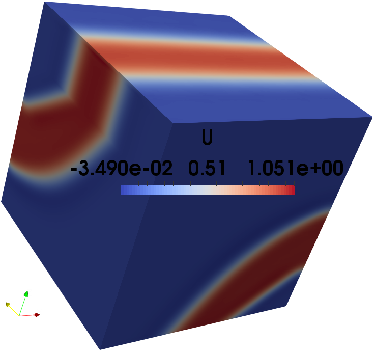
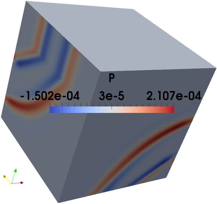
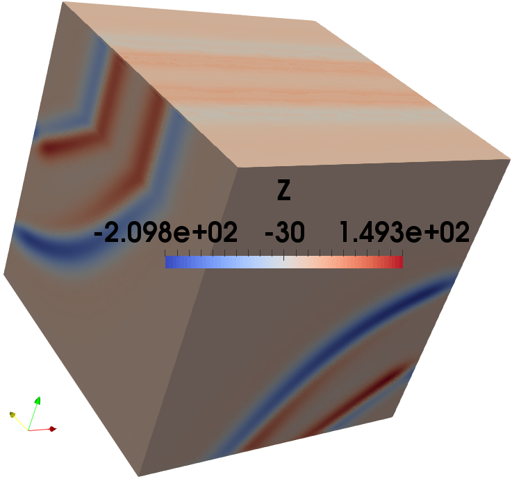
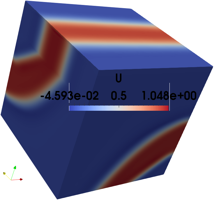
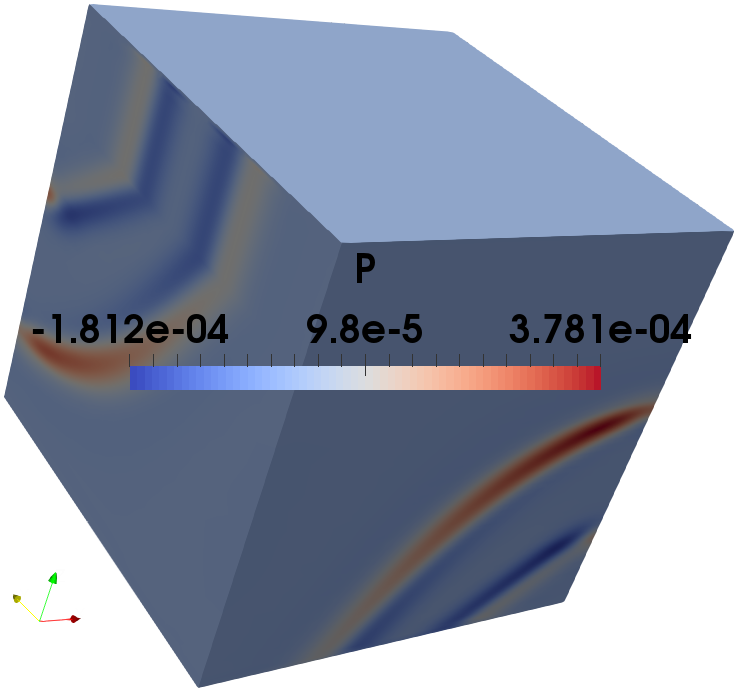
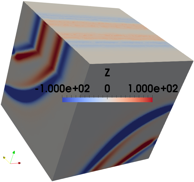
Figure 7: Example 5, visualization of the numerical solutions for state, adjoint state and control in the space-time domain: Without box constraints ($a=-1e+6$, $b=1e+6$, top), with box constraints ($a=-1e+2$, $b=1e+2$, bottom).

In Fig. 8 and Fig. 9, we visualize the numerical solutions for the state and the control at different times $t=0,\;0.25,\;0.5,\;0.75$, respectively. In this particular turning wave example, we see almost no difference between the cases with or without control constraints.

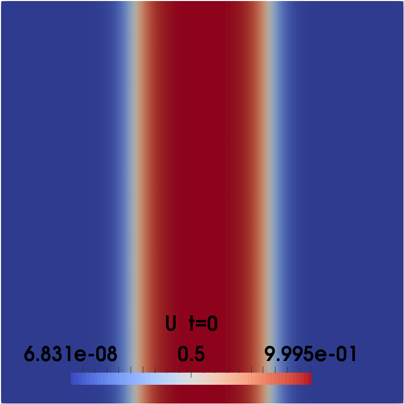
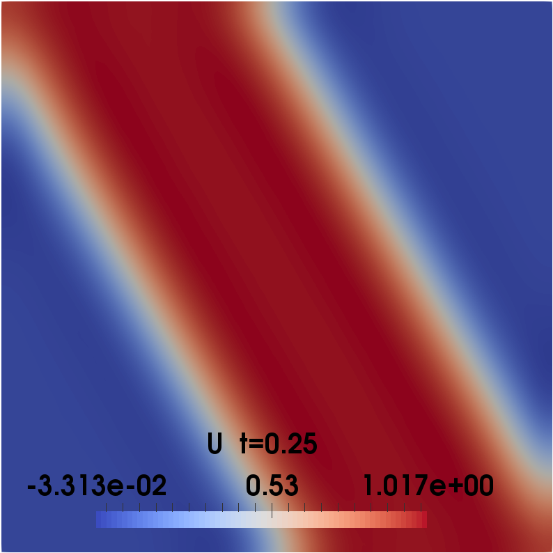
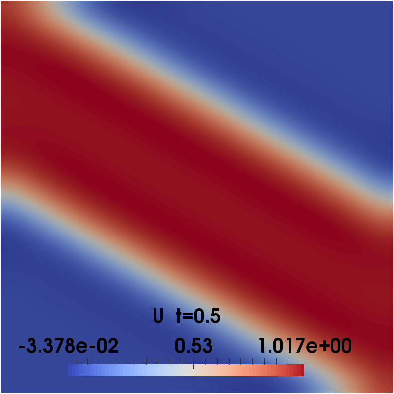
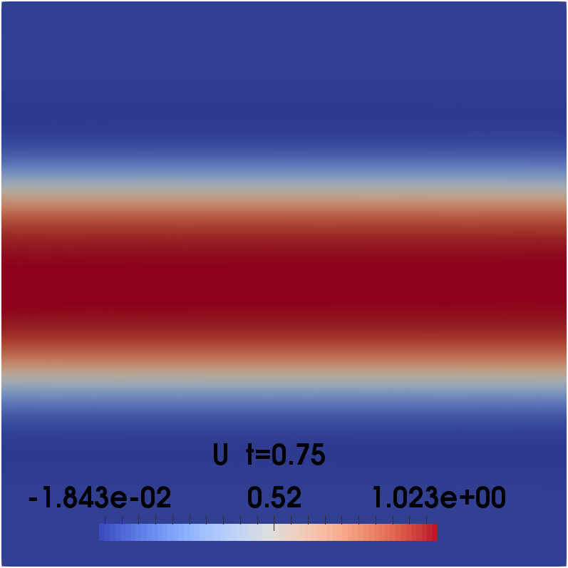
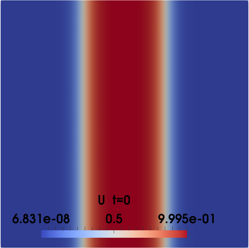
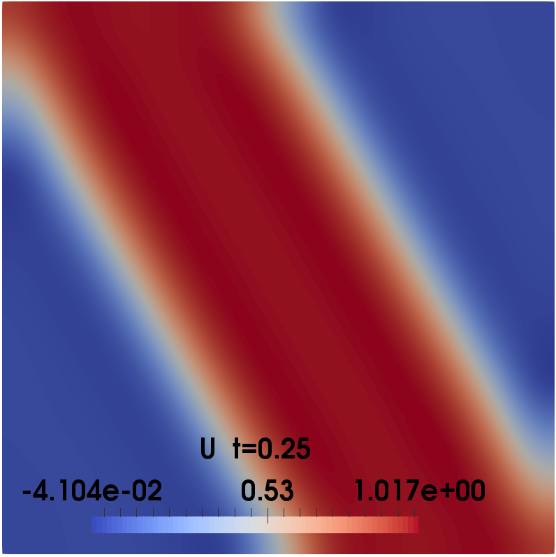
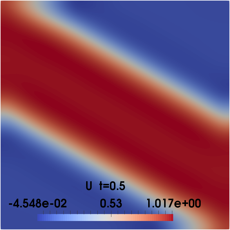
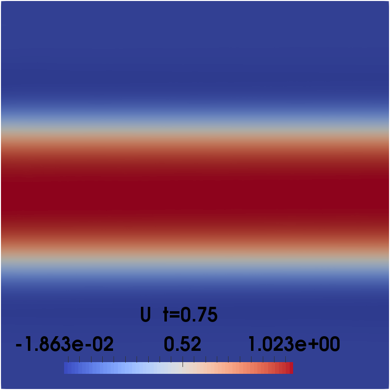
Figure 8: Example 5, visualization of the numerical solutions for the state at $t=0,\;0.25,\;0.5,\;0.75$, without box constraints ($a=-1e+6$, $b=1e+6$, top) and with box constraints ($a=-1e+2$, $b=1e+2$, bottom).

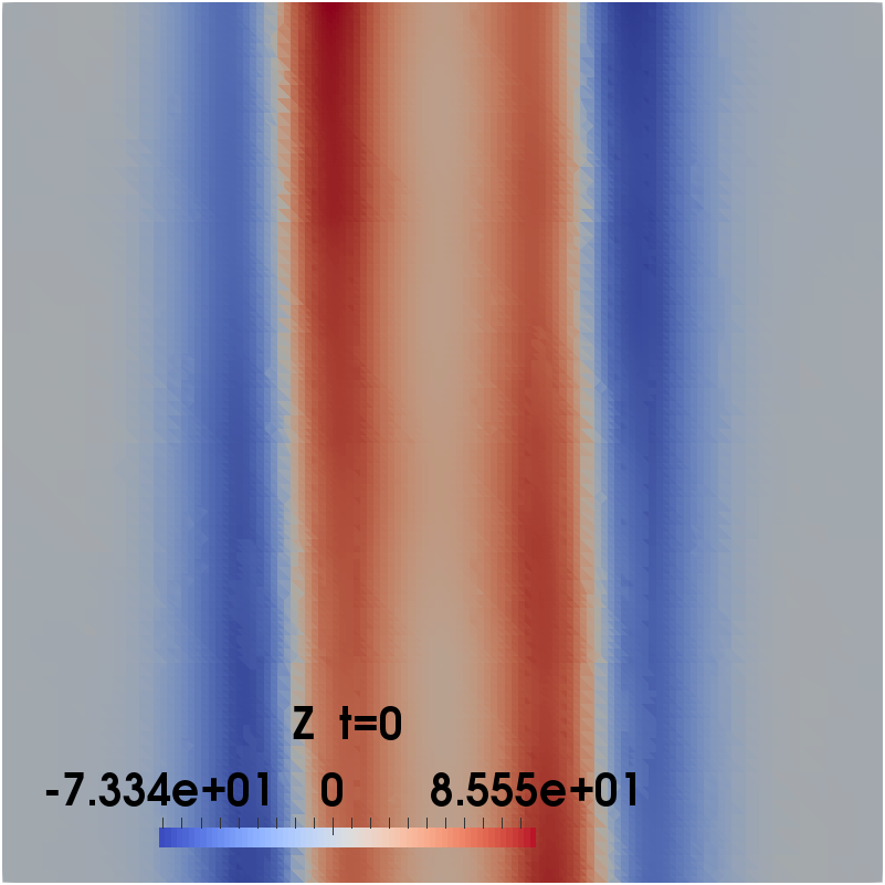
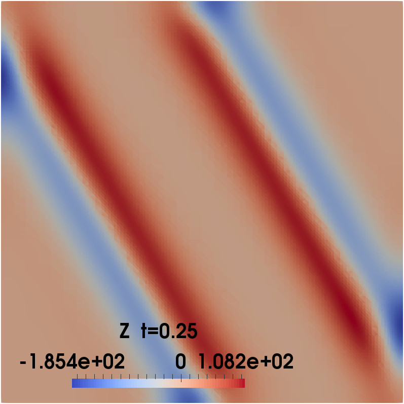
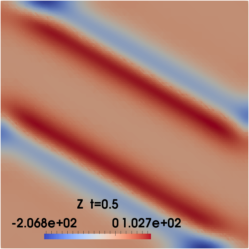
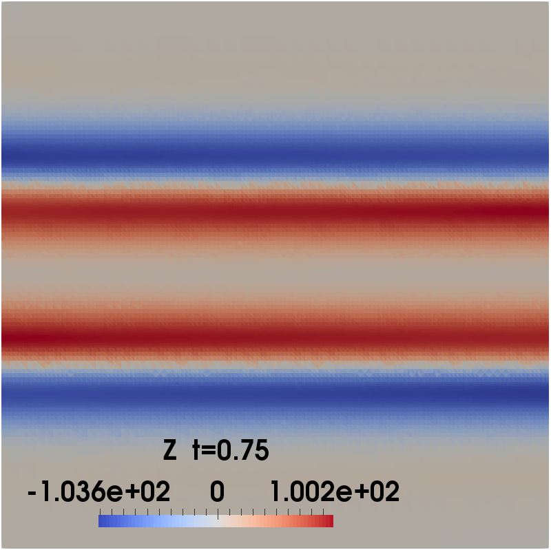
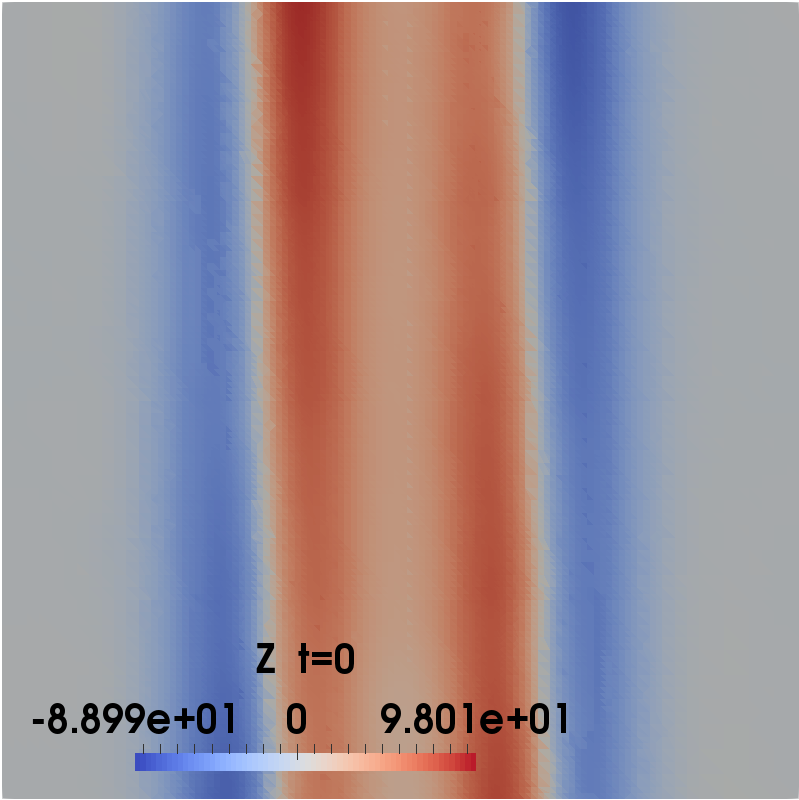
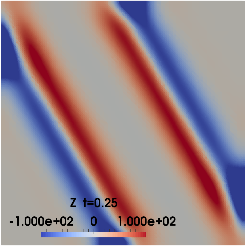
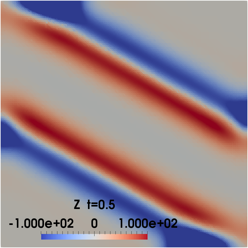
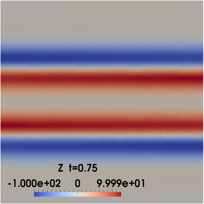
Figure 9: Example 5, visualization of the numerical solutions for the control at $t=0,\;0.25,\;0.5,\;0.75$, without box constraints ($a=-1e+6$, $b=1e+6$, top) and with box constraints ($a=-1e+2$, $b=1e+2$, bottom).

For the coupled state and adjoint state system, we applied again an adaptive method as it was used in [42] for the heat (state) equation. The adaptive meshes in the space-time domain and at different time levels $t=0,\;0.25,\;0.5,\;0.75$ are illustrated in Fig. 10. We clearly observe that our adaptive mesh refinements follow the rotation of the turning wave fronts in both the unconstrained and constrained cases. In the unconstrained problem, the mesh is visualized for the $25$th refinement step, containing $3,774,637$ grid points, i.e., $7,549,274$ degrees of freedom in total for the coupled first order necessary optimality system. In the constrained setting, the mesh is displayed for the $28$th refinement step, containing $5,100,060$ grid points, i.e., $10,200,120$ degrees of freedom in total for the coupled optimality system.

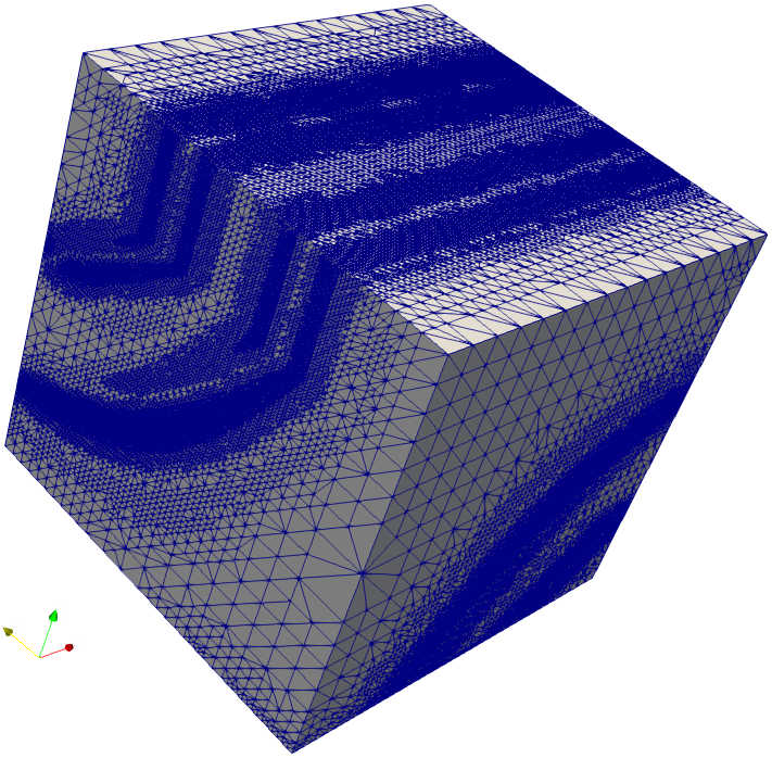
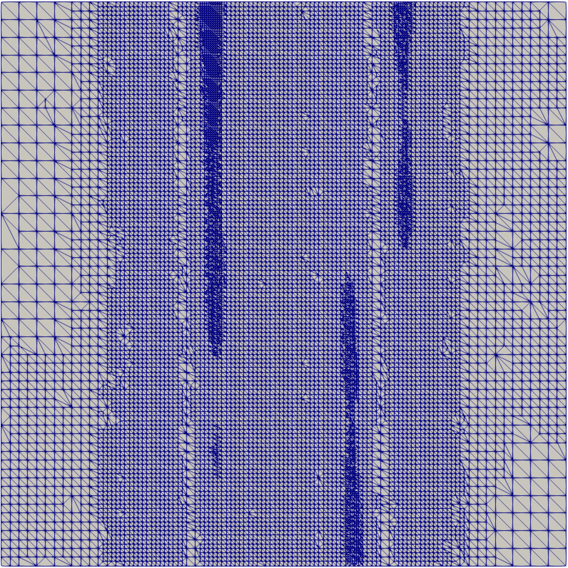
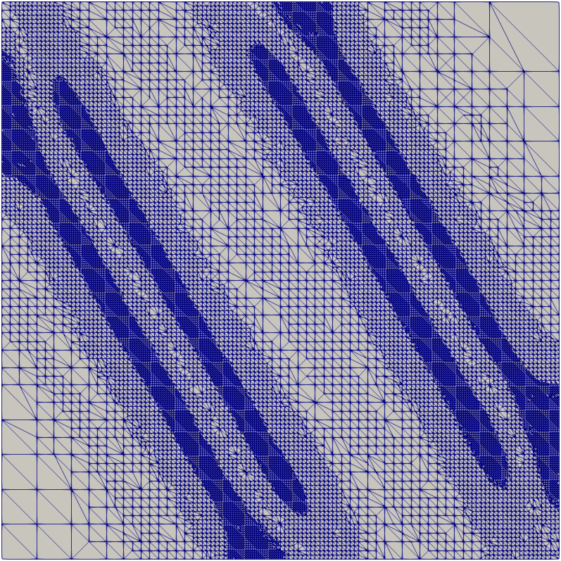
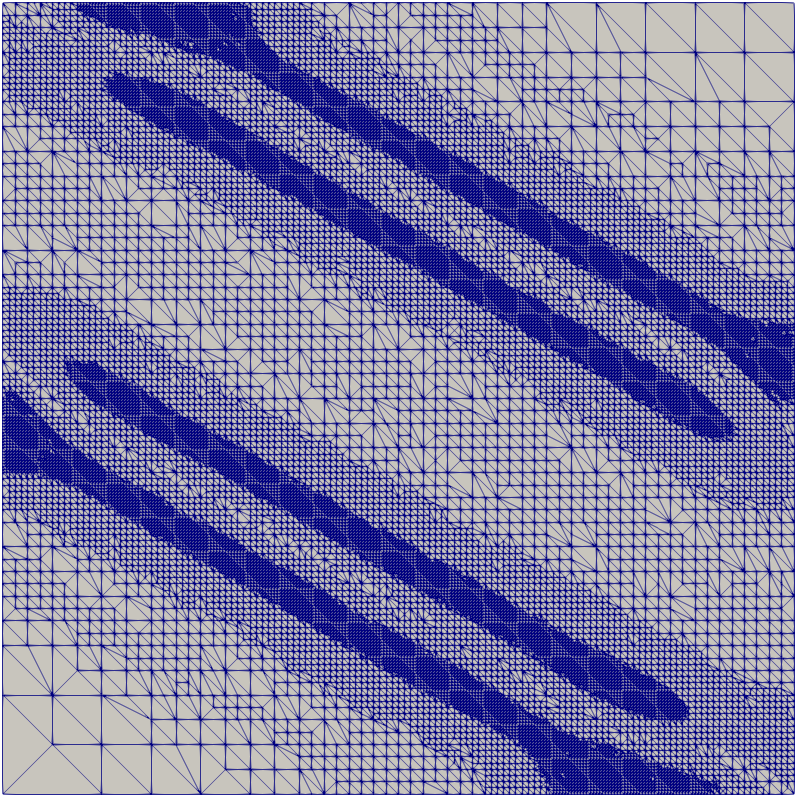
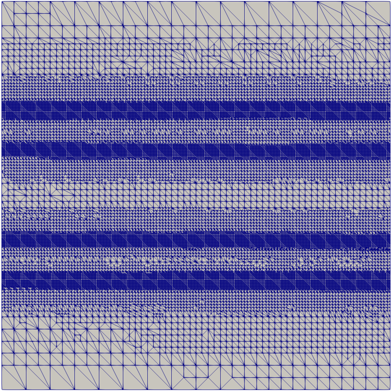
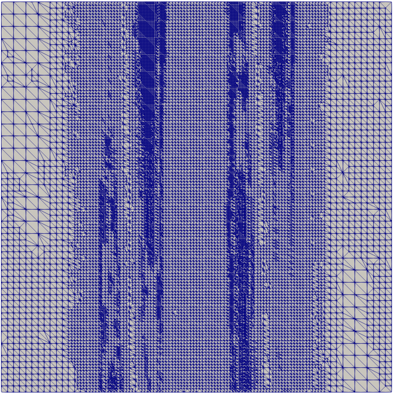
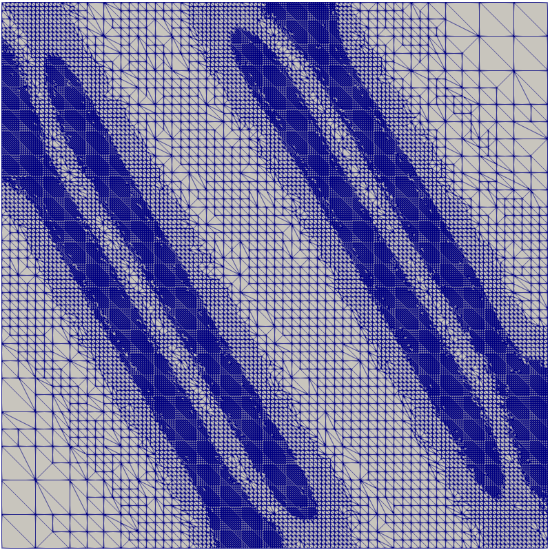
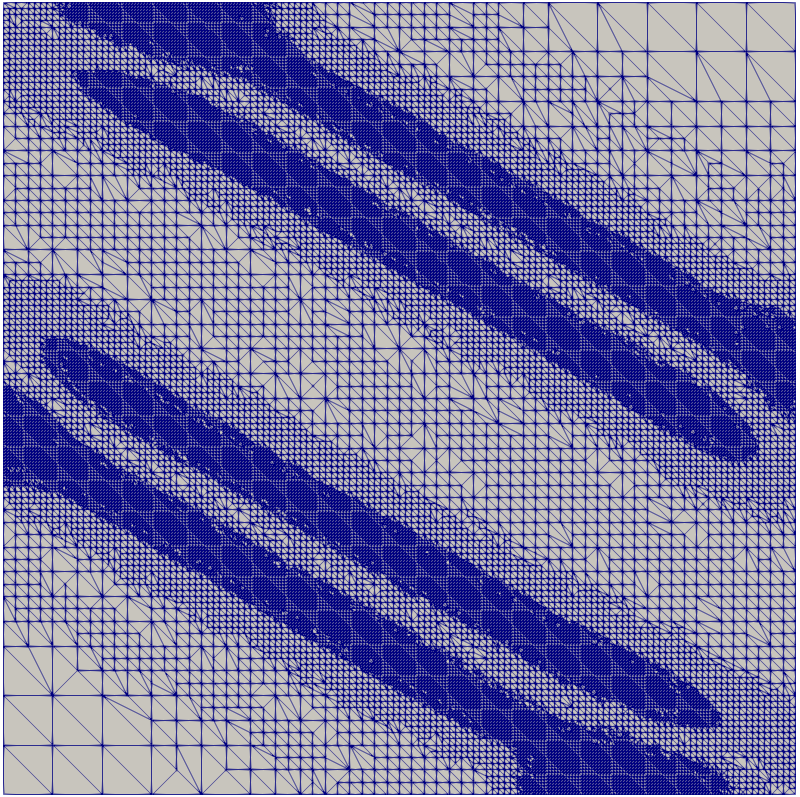
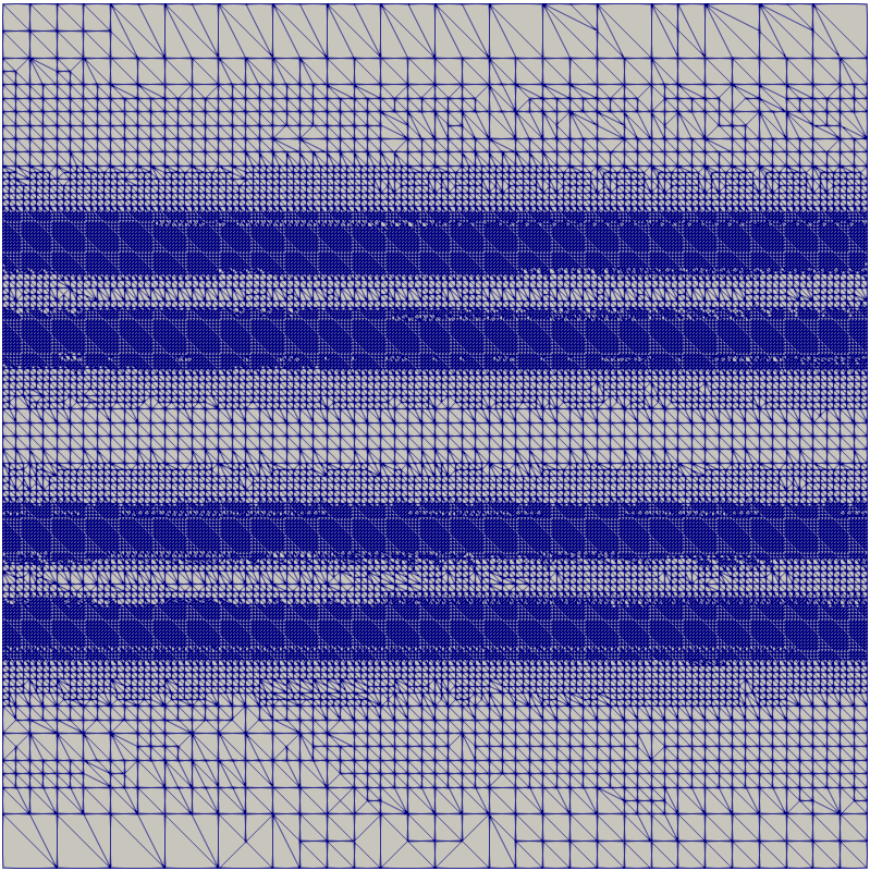
Figure 10: Example 5, visualization of the adaptive mesh refinements at the $25$th adaptive refining step without constraint (top) and the $28$th step with constraints (bottom), in the space-time domain at $t=0,\;0.25,\;0.5,\;0.75$ (from left to right)

5 Conclusions

In this work, we have considered unstructured space-time finite element methods for the optimal control of linear and semilinear parabolic equations, without or with box constraints imposed on the control. We have shown stability of the continuous and the discrete optimality system (with linear state equations and without control constraints), and derived error estimates. Our numerical results confirm the theorems and show optimal convergence rates of the space-time finite element approximations. Further, our methods are applicable to more complicated optimal control problems with semilinear state equations and box constraints. This is also confirmed by our numerical experiments, using the Lagrange-Newton method. We use adaptivity based on a residual error indicator to reduce the complexity. The rigorous analysis of adaptive space-time procedures is certainly a challenging task of future research work. The linear system respectively the linearized systems of finite element equations are solved by an algebraic multigrid preconditioned GMRES method. This GMRES works fine in practice, but a rigorous convergence analysis is still missing. The development of parallel solvers will certainly make this space-time approach an efficient alternative to time-stepping methods which are sequential in time.

References

- [1] A. Alla and S. Volkwein. Asymptotic stability of POD based model predictive control for a semilinear parabolic PDE. Adv. Comput. Math., 41(5):1073–1102, 2015.
- [2] W. Alt. The Lagrange-Newton method for infinite dimensional optimization problems. Numer. Funct. Anal. Optim., 11:201–224, 1990.
- [3] W. Alt. Sequential quadratic programming in Banach spaces. In Advances in Optimization, volume 382 of Lecture Notes in Economics and Mathematical systems, pages 281–301, New York, 1992. Springer–Verlag.
- [4] I. Babuška. Error-bounds for finite element method. Numer. Math., 16(4):322–333, 1971.
- [5] I. Babuška and A. Aziz. Survey lectures on the mathematical foundation of the finite element method. In The Mathematical Foundations of the Finite Element Method with Applications to Partial Differential Equations, pages 1–359, New York, 1972. Academic Press.
- [6] R. E. Bank, P. S. Vassilevski, and L. T. Zikatanov. Arbitrary dimension convection–diffusion schemes for space–time discretizations. J. Comput. Appl. Math., 310:19–31, 2017.
- [7] R. Becker, H. Kapp, and R. Rannacher. Adaptive finite element methods for optimal control of partial differential equations: basic concept. SIAM J. Control Optim., 39(1):113–132, 2000.
- [8] M. Behr. Simplex space-time meshes in finite element simulations. Int. J. Numer. Methods Fluids, 57:1421–1434, 2008.
- [9] J. Bey. Tetrahedral grid refinement. Computing, 55:355–378, 1995.
- [10] A. Borzì and V. Schulz. Computational optimization of systems governed by partial differential equations, volume 8 of Computational Science & Engineering. Society for Industrial and Applied Mathematics (SIAM), Philadelphia, PA, 2012.
- [11] D. Braess. Finite Elements: Theory, Fast Solvers, and Applications in Solid Mechanics. Cambridge University Press, 2007.
- [12] A. Bünger, S. Dolgov, and M. Stoll. A low-rank tensor method for PDE-constrained optimization with isogeometric analysis. SIAM J. Sci. Comput., 42(1):A140–A161, 2020.
- [13] E. Casas, M. Mateos, and A. Rösch. Approximation of sparse parabolic control problems. Math. Control Relat. Fields, 7(3):393–417, 2016.
- [14] E. Casas, C. Ryll, and F. Tröltzsch. Sparse optimal control of the Schlögl and FitzHugh-Nagumo systems. Comput. Methods Appl. Math., 13(4):415–442, 2013.
- [15] E. Casas, C. Ryll, and F. Tröltzsch. Second order and stability analysis for optimal sparse control of the FitzHugh-Nagumo equation. SIAM J. Control Optim., 53(4):2168–2202, 2015.
- [16] E. Casas, C. Ryll, and F. Tröltzsch. Optimal control of a class of reaction diffusion equations. Comput. Optim. Appl., 70(3):677–707, 2018.
- [17] P. Deuflhard. Newton methods for nonlinear problems, volume 35 of Springer Series in Computational Mathematics. Springer, Heidelberg, 2011.
- [18] A. Ern and J.-L. Guermond. Theory and Practice of Finite Elements. Springer-Verlag, New Year, 2004.
- [19] M. J. Gander. 50 years of time parallel integration. In Multiple Shooting and Time Domain Decomposition, pages 69–114. Springer Verlag, Heidelberg, Berlin, 2015.
- [20] W. Gong, M. Hinze, and Z. Zhou. Space-time finite element approximation of parabolic optimal control problems. J. Numer. Math., 20(2):111–145, 2012.
- [21] S. Götschel and M. Minion. An efficient parallel-in-time method for optimization with parabolic PDEs. SIAM J. Sci. Comput., 41(6):C603–C626, 2019.
- [22] M. Gunzburger and A. Kunoth. Space-time adaptive wavelet methods for optimal control problems constrained by parabolic evolution equations. SIAM J. Control Optim., 49(3):1150–1170, 2011.
- [23] W. Hackbusch. Numerical solution of linear and nonlinear parabolic control problems. In A. Auslender, W. Oettli, and J. Stoer, editors, Optimization and Optimal Control. Lecture Notes in Control and Information Sciences, volume 30 of Lecture Notes in Control and Information Sciences, pages 179–185. Springer, Berlin, Heidelberg, 1981.
- [24] M. Hintermüller, M. Hinze, C. Kahle, and T. Keil. A goal-oriented dual-weighted adaptive finite element approach for the optimal control of a nonsmooth Cahn-Hilliard-Navier-Stokes system. Optim. Eng., 19(3):629–662, 2018.
- [25] M. Hinze, R. Pinnau, M. Ulbrich, and S. Ulbrich. Optimization with PDE Constraints, volume 23. Springer-Verlag, Berlin, 2009.
- [26] K. Ito and K. Kunisch. Lagrange Multiplier Approach to Variational Problems and Applications. SIAM, Philadelphia, 2008.
- [27] V. Karyofylli, L. Wendling, M. Make, N. Hosters, and M. Behr. Simplex space-time meshes in thermally coupled two-phase flow simulations of mold filling. Comput. Fluids, page 104261, 2019.
- [28] M. Kollmann, M. Kolmbauer, U. Langer, M. Wolfmayr, and W. Zulehner. A finite element solver for a multiharmonic parabolic optimal control problem. Comput. Math. Appl., 65:469–486, 2013.
- [29] K. Kunisch, S. Volkwein, and L. Xie. HJB-POD-based feedback design for the optimal control of evolution problems. SIAM J. Appl. Dyn. Syst., 3(4):701–722, 2004.
- [30] A. Kunoth. Wavelet methods—elliptic boundary value problems and control problems. Advances in Numerical Mathematics. B. G. Teubner, Stuttgart, 2001.
- [31] O. A. Ladyzhenskaya. The boundary value problems of mathematical physics, volume 49 of Applied Mathematical Sciences. Springer-Verlag, New York, 1985. Translated from the Russian edition, Nauka, Moscow, 1973.
- [32] O. A. Ladyzhenskaya, V. A. Solonnikov, and N. Uraltseva. Linear and quasi-linear equations of parabolic type. AMS, USA, 1968. Translated from the Russian edition, Nauka, Moscow, 1967.
- [33] U. Langer, M. Neumüller, and A. Schafelner. Space-time finite element methods for parabolic evolution problems with variable coefficients. In T. Apel, U. Langer, A. Meyer, and O. Steinbach, editors, Advanced Finite Element Methods with Applications: Selected Papers from the 30th Chemnitz Finite Element Symposium 2017, pages 247–275, Cham, 2019. Springer International Publishing.
- [34] U. Langer, S. Repin, and M. Wolfmayr. Functional a posteriori error estimates for time-periodic parabolic optimal control problems. Numer. Func. Anal. Opt., 37(10):1267–1294, 2016.
- [35] J. Lions, Y. Maday, and G. Turinici. A ”parareal” in time discretization of PDE’s. Comptes Rendus de l’Académie des Sciences, Série I, 323(7):661–668, 2015.
- [36] J. L. Lions. Contrôle optimal de systèmes gouvernés par des équations aux dérivées partielles. Dunod Gauthier-Villars, Paris, 1968.
- [37] D. Meidner and B. Vexler. A priori error estimates for space-time finite element discretization of parabolic optimal control problems. Part I: Problems without control constraints. SIAM J. Control Optim., 47(3):1150–1177, 2008.
- [38] D. Meidner and B. Vexler. A priori error estimates for space-time finite element discretization of parabolic optimal control problems. Part II: Problems with control constraints. SIAM J. Control Optim., 47(3):1301–1329, 2008.
- [39] C. Meyer and A. Rösch. Superconvergence properties of optimal control problems. SIAM J. Control Optim., 43(3):970–985, 2004.
- [40] J. Nečas. Sur une méthode pour résoudre les équations aux dérivées partielles du type elliptique, voisine de la variationnelle. Ann. Scuola Norm. Sup. Pisa, 16(4):305–326, 1962.
- [41] O. Steinbach. Space-time finite element methods for parabolic problems. Comput. Methods Appl. Math., 15:551–566, 2015.
- [42] O. Steinbach and H. Yang. Comparison of algebraic multigrid methods for an adaptive space-time finite-element discretization of the heat equation in 3d and 4d. Numer. Linear Algebra Appl., 25(3):e2143, 2018.
- [43] O. Steinbach and H. Yang. Space-time finite element methods for parabolic evolution equations: discretization, a posteriori error estimation, adaptivity and solution. In O. Steinbach and U. Langer, editors, Space-Time Methods: Application to Partial Differential Equations, Radon Series on Computational and Applied Mathematics, pages 207–248, Berlin, 2019. de Gruyter.
- [44] V. Thomée. Galerkin finite element methods for parabolic problems, volume 25 of Springer Series in Computational Mathematics. Springer-Verlag, Berlin, second edition, 2006.
- [45] F. Tröltzsch. On the Lagrange-Newton-SQP method for the optimal control of semilinear parabolic equations. SIAM J. Control Optim., 38:294–312, 1999.
- [46] F. Tröltzsch. Optimal control of partial differential equations: Theory, methods and applications, volume 112 of Graduate Studies in Mathematics. American Mathematical Society, Providence, Rhode Island, 2010.
- [47] S. Ulbrich. Generalized SQP methods with “parareal” time-domain decomposition for time-dependent PDE-constrained optimization. In Real-time PDE-constrained optimization, volume 3 of Comput. Sci. Eng., pages 145–168. SIAM, Philadelphia, PA, 2007.
- [48] E. Zeidler. Nonlinear Functional Analysis and its Applications II/B: Nonlinear Monotone Operators. Springer, New York, 1990.