The Hubble stream near a massive object: the exact analytical solution for the spherically-symmetric case

Abstract

The gravitational field of a massive object (for instance, of a galaxy group or cluster) disturbs the Hubble stream, decreasing its speed. Dependence $v(r_{0})$ of the radial velocity of the stream from the present-day radius $r_{0}$ can be directly observed and may provide valuable information about the cluster properties. We offer an exact analytical relationship $v(r_{0})$ for a spherically-symmetric system.

I Introduction

In an ideal Friedmann’s universe, all nearby objects move off radially from an observer with the speed proportional to the distance to the object (the famous Hubble-Lemaître law). The real Universe, however, contains local overdensities (like galaxy groups or clusters), and their additional gravitational attraction slows down the Hubble flow, changing the dependence $v(r_{0})$ of the radial velocity from the present-day radius $r_{0}$. Hereafter we will consider a single overdensity and name it the ’galaxy cluster’, though our reasoning is equally valid for any cosmological object, on condition that the suppositions that we will make during the derivation are applicable for the object. The dependence $v(r_{0})$ can be obtained from observations (see, for instance, Figure 1 in Karachentsev et al. (2009))) and, in principle, may tell a lot about the cluster and its environment. We just need to build a theoretical model of $v(r_{0})$ as a function of cluster parameters and compare it with observations.

Of course, the task is well-known, and there is a vast literature dedicated to its solution. The methods can be roughly divided into three groups. The analytical approach was applied in old papers (for example, Olson and Silk (1979); Lynden-Bell (1981); Giraud (1986)), but the cosmological constant was believed to be zero at that time. Several approximative formulas were offered for $v(r_{0})$ (for instance, Peirani and de Freitas Pacheco (2008); Karachentsev et al. (2009)). Recently N-body simulations are performed to solve the problem (e.g., Hanski et al. (2001); Peñarrubia et al. (2014)), which allowed to consider realistic non-spherical models of the Local Group.

On the other hand, the N-body simulations may not be considered as having no disadvantages Baushev et al. (2017); Baushev and Barkov (2018); Baushev and Pilipenko (2020), and the analytical approach seems preferable in simple cases, since it allows to obtain a precise and compact equation for $v(r_{0})$. For instance, Baushev (2019) offered an exact analytical equation for the radius $L_{0}$, at which a spherically-symmetric object of mass $M$ stops the Hubble flow, i.e., $v(L_{0})=0$. We use the same approach in this letter, and our aim is to generalize the result of Baushev (2019) and find the full velocity profile $v(r_{0})$ in the spherically-symmetric case. As we will see, one may find an exact analytical solution of this task, even for an arbitrary (but spherically-symmetric) distribution of matter around the cluster.

Let us specify the Universe model, which is implied in this Letter. We suppose that the Universe is homogeneous and isotropic, i.e., its metrics can be represented as $ds^{2}=c^{2}dt^{2}-a^{2}(t)dl^{2}$, where $dl$ is an element of three-dimensional length and $a$ is the scale factor of the Universe. We denote the present-day values of the Hubble constant, critical density, and the scale factor of the Universe by $H_{0}$, $\rho_{c,0}$, and $a_{0}$, respectively. We denote the present-day matter, dark energy, and curvature densities of the Universe by $\rho_{M,0}$, $\rho_{\Lambda,0}$, $\rho_{a,0}$, respectively. We may also introduce the ratios of the present-day densities of the universe components to $\rho_{c,0}$: $\Omega_{a,0}\equiv\rho_{a,0}/\rho_{c,0}$ etc. In the literature, the quantities $\Omega_{\Lambda,0}$, $\Omega_{M,0}$ etc. are often denoted simply by $\Omega_{\Lambda}$, $\Omega_{M}$ etc., but we use the additional sub-index to remind that these are the present-day values.

We perform our calculations for the case of the standard $\Lambda$CDM Universe (though they can be easily generalized for less standard cosmological models). We suppose that the dark energy behaves simply as the cosmological constant (i.e., $p_{\Lambda}=-\rho_{\Lambda,0}=\it{const}$), and that the Universe is flat ($\Omega_{a,0}=0$) in absence of structures Tanabashi et al. (2018). We neglect the contribution of the radiation component: the present-day density of radiation is $\sim 10^{-4}\rho_{c,0}$, and, though the contribution was much larger in the early Universe, we will show that the relative error of the velocity field determination caused by the disregarding of radiation is also $\sim 10^{-4}$. Then we obtain: $\Omega_{\Lambda,0}+\Omega_{M,0}=1$. The universe age $t_{0}$ in the $\Lambda$CDM is defined by the well-known equation (see e.g. (Gorbunov and Rubakov, 2011, eqn. 4.29)):

$$t_{0}H_{0}\sqrt{\Omega_{\Lambda,0}}=\frac{2}{3}\operatorname{arcosh}\left(1/\sqrt{\Omega_{M,0}}\right)$$ (1)

We may obtain this equation from (2), if we substitute there $\sigma_{M,0}=\Omega_{M,0}\rho_{c,0}$, $\sigma_{\Lambda,0}=\Omega_{\Lambda,0}\rho_{c,0}$, $\sigma_{a,0}=0$ and integrate.

II The idea of the solution

We find the velocity field around a cluster of galaxies under the following assumptions:

1. The system is spherically-symmetric and has not experienced any tidal perturbations from other structures.

2. Its characteristic radius (for instance, we may consider $R_{0}$) is much larger than its gravitational radius and much smaller than the universe radius ($c/H_{0}\gg R_{0}\gg R_{g}\equiv{2GM}/{c^{2}}$). The significance of this assumption will be explained below.

We choose the center of symmetry of the system as the origin of coordinates, and the Big Bang as the zero point of time. We denote the present-day radii and radial speeds of the objects around the cluster by $r_{0}$ and $v$. We emphasize that $v$ is the speed of the Hubble stream, it is refined from the peculiar velocities of the objects. Our aim is to find the relationship $v(r_{0})$.

Consider a spherical layer of radius $r_{0}$ and determine its previous evolution $r(t,r_{0})$. Our solution is based on two well-known properties of spherically-symmetric gravitating systems in the general theory of relativity: first, a spherically-symmetric distribution outside a radius $r$ does not create any gravitational field inside this radius. It means that the matter outside $r$ does not affect the dependence $r(t,r_{0})$ at all.

Second, $r(t,r_{0})$ depends only on the total mass of dark and baryonic matter inside $r$, and does not depend on the matter space distribution, if the distribution is spherically-symmetric. Indeed, the exterior layers do not create any gravitational field at $r$, and, in accordance with the Birkhoff’s theorem, the gravitational field created at $r$ by the spherical, nonrotating matter inside $r$ must be Schwarzschild, i.e., it depends on the only parameter, the total energy inside $r$. Contrary to the newtonian gravity, the gravitational field in the general theory of relativity is created by both, density and pressure. However, the only component with significant pressure in our system is the dark energy, which has exactly the same pressure and density everywhere. The matter pressure is negligible with respect to its density. Therefore, the total mass inside $r$ does not depend on the matter distribution inside $r$, and we may redistribute the matter inside $r$ whatever we like without any influence on the gravitational force at $r$ and the layer evolution $r(t,r_{0})$.

III Calculations

Thus, we may virtually redistribute the matter inside $r$ uniformly, and it will not affect the dependence $r(t,r_{0})$. But then we have a ’uniform universe’ inside $r$, and its evolution may be found from the usual Friedmann equation (see e.g. (Gorbunov and Rubakov, 2011, eqn. 4.1)):

$$\left(\dfrac{dr}{rdt}\right)^{2}=\dfrac{H^{2}_{0}}{\rho_{c,0}}\left[\sigma_{M,0}\left(\dfrac{r_{0}}{r}\right)^{3}\!\!+\sigma_{\Lambda,0}+\sigma_{a,0}\left(\dfrac{r_{0}}{r}\right)^{2}\right].$$ (2)

Here $\sigma_{M,0}$, $\sigma_{\Lambda,0}$, $\sigma_{a,0}$ are the averaged present-day matter, dark energy, and curvature densities inside $r_{0}$. Of course, $\sigma_{M,0}$, $\sigma_{\Lambda,0}$, $\sigma_{a,0}$ depend on $r_{0}$. By analogy with $\Omega_{0}$, we may introduce the fractions $\Sigma_{M,0}\equiv\sigma_{M,0}/\rho_{c,0}$ etc. We purposefully use $\sigma$ and $\Sigma$ in order to distinguish the averaged densities $\sigma$ and $\Sigma$, depending on $r_{0}$, from $\rho$ and $\Omega$, that correspond to the undisturbed Universe and therefore are universal. Obviously, $\sigma_{\Lambda,0}=\rho_{\Lambda,0}$, $\Sigma_{\Lambda,0}=\Omega_{\Lambda,0}$. Denoting the matter mass as a function of $r_{0}$ by $M_{M}(r_{0})$, we obtain

$$\Sigma_{M,0}(r_{0})=\dfrac{3M_{M}(r_{0})}{4\pi r^{3}_{0}\rho_{c,0}}.$$ (3)

Here we used assumption 2 about the cluster of galaxies: it implies that the space near the cluster is flat. At $r=r_{0}$ $dr/dt=v(r_{0})$, and we obtain from (2)

$$\left(\dfrac{v}{r_{0}H_{0}}\right)^{2}=\left[\Sigma_{M,0}+\Omega_{\Lambda,0}+\Sigma_{a,0}\right]$$

$$\Sigma_{a,0}=\left(\dfrac{v}{r_{0}H_{0}}\right)^{2}-\Sigma_{M,0}-\Omega_{\Lambda,0}$$ (4)

We substitute this value to (2) and obtain

$$\left(\frac{dx}{H_{0}dt}\right)^{2}=\frac{\Sigma_{M,0}}{x}(1-x)-\Omega_{\Lambda,0}(1-x^{2})+\left(\frac{v}{r_{0}H_{0}}\right)^{2},$$ (5)

where $x\equiv r/r_{0}$. We introduce two new designations

$$\alpha=\frac{\Sigma_{M,0}}{\Omega_{\Lambda,0}};\qquad U=\frac{v^{2}_{0}}{r^{2}_{0}H^{2}_{0}\Omega_{\Lambda,0}}.$$ (6)

As we can see, $U\geq 0$. Strictly speaking, $\alpha$ and $U$ are functions of $r_{0}$, but now it is more convenient for us now to consider them as independent variables. We may rewrite (5) as

$$H_{0}\sqrt{\Omega_{\Lambda,0}}dt=\frac{\sqrt{x}dx}{\sqrt{x^{3}+(U-\alpha-1)x+\alpha}}\equiv\xi(U,\alpha,x)dx.$$ (7)

Here we introduced a new function $\xi(U,\alpha,x)$

$$\xi(U,\alpha,x)\equiv\dfrac{\sqrt{x}}{\sqrt{x^{3}+(U-\alpha-1)x+\alpha}}$$ (8)

for brevity sake. Variables $\alpha$ and $U$ do not depend on $x$, and we may easily integrate equation (7). If $v\geq 0$ (obviously, it means that $r_{0}\geq L_{0}$), the integration is trivial:

$$t_{0}H_{0}\sqrt{\Omega_{\Lambda,0}}=\int_{0}^{1}\xi(U,\alpha,x)dx.$$ (9)

Comparing this equation with (1), we equate their right parts:

$$\frac{2}{3}\operatorname{arcosh}\left(1/\sqrt{\Omega_{M,0}}\right)=\int_{0}^{1}\xi(U,\alpha,x)dx,\quad\text{if }v\geq 0.$$ (10)

This equation defines $U$ as an implicit function of $\alpha$ and $\Omega_{M,0}$. The function can be resolved with respect to $U$ in form of an explicit function $U_{+}(\alpha,\Omega_{M,0})$. The subscript ’$+$’ reminds that the function describes only the positive velocity branch, or $r_{0}\geq L_{0}$. We should underline that equation (10) gives a meaningful relation $U_{+}(\alpha,\Omega_{M,0})$ not for all pairs of $U$ and $\alpha$. This issue will be discussed in section IV.

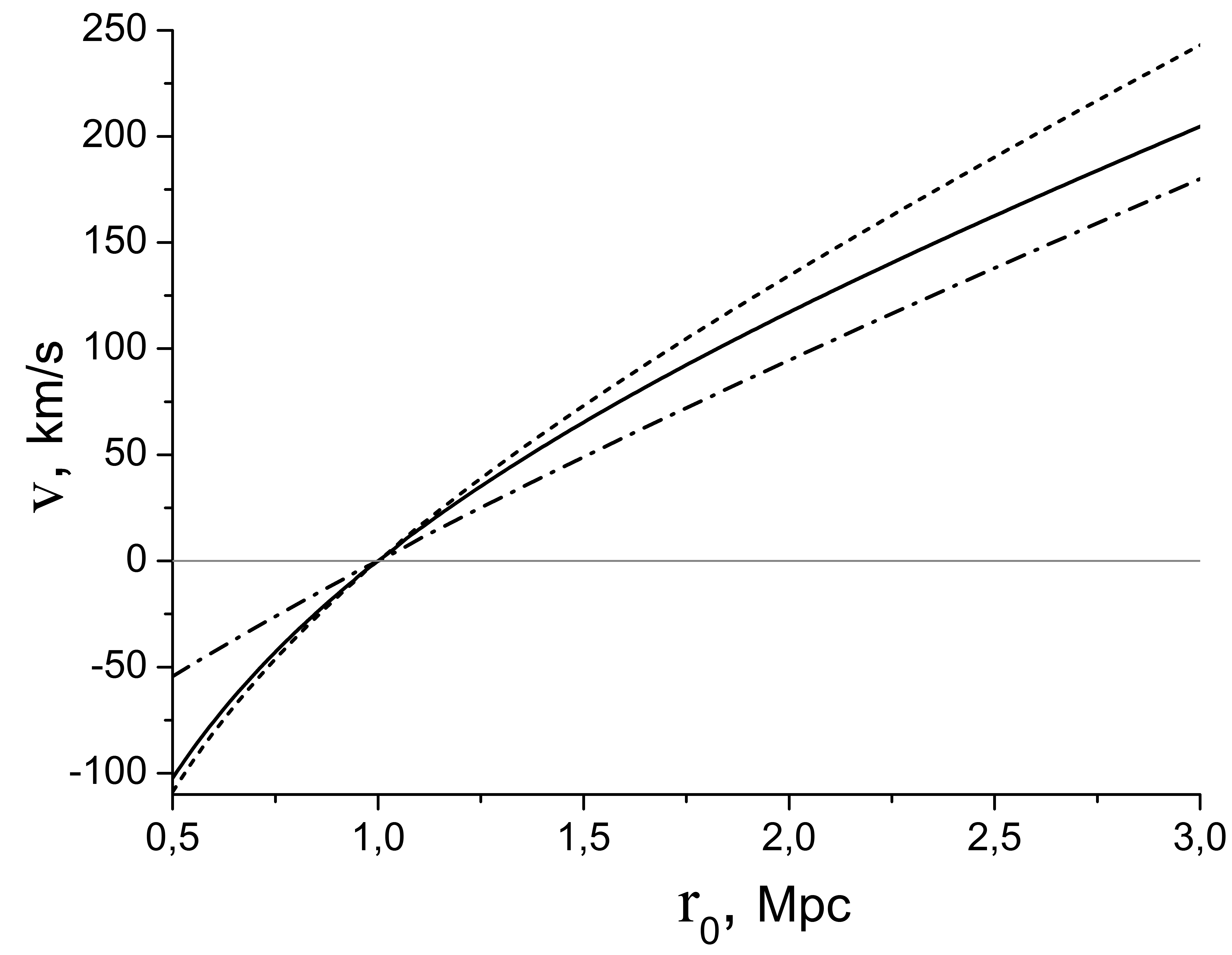
Figure 1: The speed profiles of the Hubble stream around the cluster for the point model (17) (solid line), halo model (18) (dash-dot line), and empty model (19) (dot line), respectively, at the distances $0.5-3$ Mpc from the cluster center.

If we substitute $U=0$ into (10), we obtain an implicit function, bounding the average matter density inside the stop radius $L_{0}$, namely $\alpha_{0}=\Sigma_{M,0}/\Omega_{\Lambda,0}$, with $\Omega_{M,0}$:

$$\frac{2}{3}\operatorname{arcosh}\left(1/\sqrt{\Omega_{M,0}}\right)=\int_{0}^{1}\frac{\sqrt{x}dx}{\sqrt{x^{3}-(\alpha_{0}+1)x+\alpha_{0}}}.$$ (11)

This equation coincides with equation (11) from Baushev (2019) and allows to find $L_{0}$ for an arbitrary spherically-symmetric mass distribution $M(r_{0})$ (see Baushev (2019) for details).

The integration of (7) is more complex, if $v<0$ (i.e., $r_{0}<L_{0}$). In this case, the toy ’uniform universe’ inside $r$, which we consider, has already passed its maximum expansion and now contracts (therefore $v<0$). The maximum expansion $x_{max}=r_{max}/r_{0}$ corresponds to the moment when $dr/dt=0$ (or $dx/dt=0$), i.e., the radicand in (7) turns to zero. Thus $x_{max}$ is a root of the equation $x^{3}+(U-\alpha-1)x+\alpha=0$. Since $x$ varies from $0$ to $x_{max}$, we should choose the smallest real positive one. Actually, the root should exceed $1$ (since the ’universe’ contracts, its maximum radius $r_{max}$ should exceed the present-day radius $r_{0}$). A cubic equation has three roots, and two of them can be complex. However, expression $f(x)=x^{3}+(U-\alpha-1)x+\alpha$ is equal to $\alpha>0$ at $x=0$, and $f(x)\to-\infty$ if $x\to-\infty$. Consequently, one of the real roots is obligatory negative and cannot be $x_{max}$. Thus, $x_{max}$ exists only if all three roots of the equation are real. It is easy to show that we should choose the middle one:

$$x_{max}=\dfrac{\left(1-i\sqrt{3}\right)(U-\alpha-1)}{3\cdot 2^{2/3}\cdot\left(-\alpha+\sqrt{27\alpha^{2}+4(U-\alpha-1)^{3}}\right)^{1/3}}-$$

$$-\dfrac{\left(1+i\sqrt{3}\right)\left(-\alpha+\sqrt{27\alpha^{2}+4(U-\alpha-1)^{3}}\right)^{1/3}}{2^{4/3}}.$$ (12)

If $x_{max}$ obtained with this equation for some pair of $U$ and $\alpha$ is not real or $x_{max}<1$, it means that $v$ cannot be negative for these values of $U$ and $\alpha$. We will specify the necessary conditions in section IV.

Thus, if $v<0$, the right part of (7) should be integrated from $x=0$ to $x=x_{max}$, and then from $x=x_{max}$ to $x=1$:

$$t_{0}H_{0} \sqrt{\Omega_{\Lambda,0}}=\int\limits_{0}^{x_{max}}\xi(U,\alpha,x)dx+\int\limits_{1}^{x_{max}}\xi(U,\alpha,x)dx=$$

$$= 2\int\limits_{0}^{x_{max}}\xi(U,\alpha,x)dx-\int\limits_{0}^{1}\xi(U,\alpha,x)dx,\text{if }v<0.$$ (13)

Comparing this equation with (1), we equate their right parts and obtain the final solution for the $v<0$ case:

$$\frac{2}{3}\operatorname{arcosh}\left(1/\sqrt{\Omega_{M,0}}\right)=$$

$$=2\int\limits_{0}^{x_{max}}\xi(U,\alpha,x)dx-\int\limits_{0}^{1}\xi(U,\alpha,x)dx,\text{if }v<0.$$ (14)

We derive equations (10) and (14) equating the universe ages, and justifies the disregard of the radiation term in the Friedmann equation. Radiation dominated in the early Universe, but for less than $10^{-4}$ of the Universe age ($<5\cdot 10^{5}$ years). For almost all of the $13.6$ bln. years the Universe has been living with the fraction of radiation, comparable with the present-day one ($\Omega_{\gamma,0}<10^{-4}$), and we may conclude that the relative error occurring from the neglect of the radiation term does not exceed $10^{-4}$.

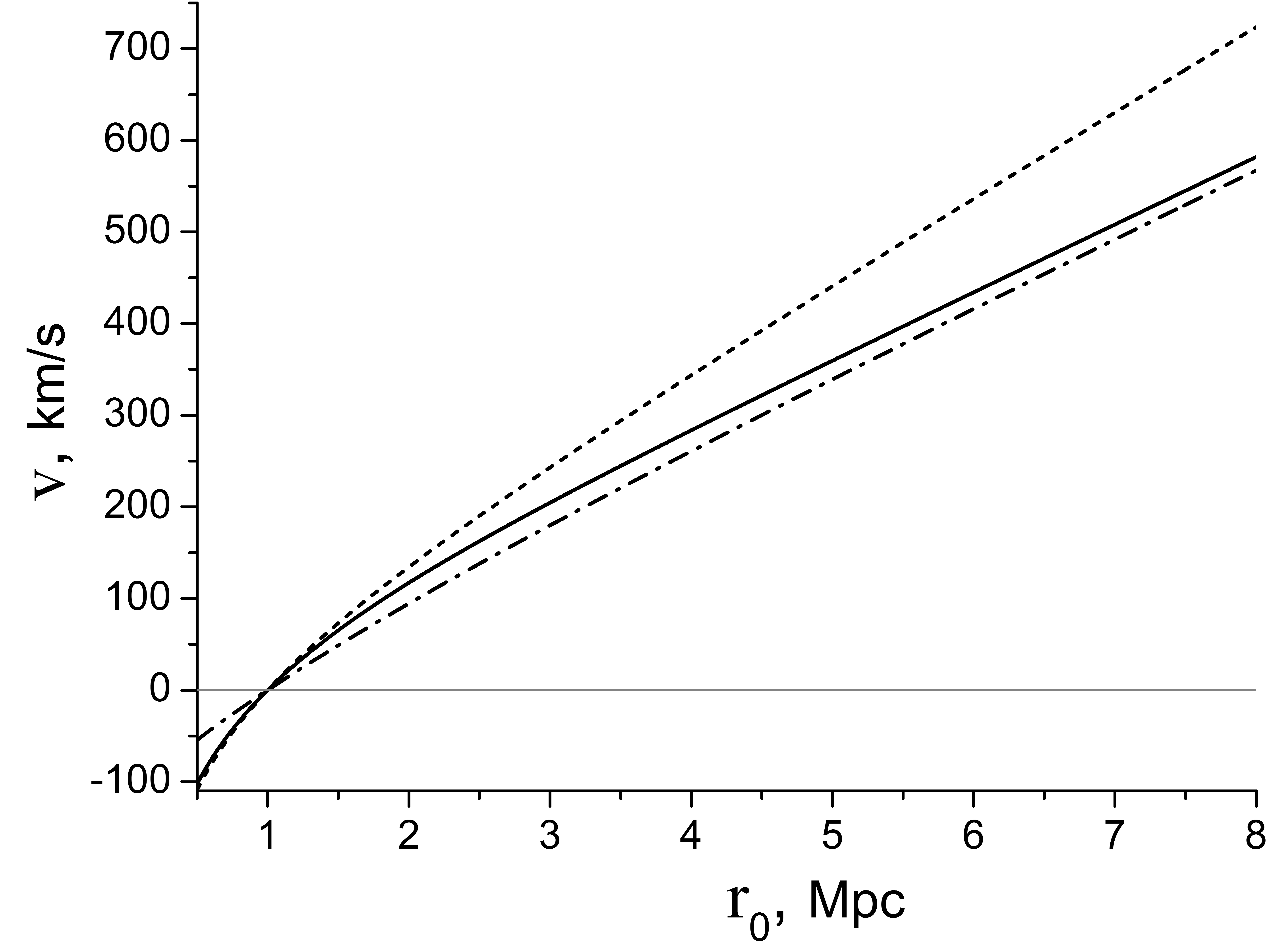
Figure 2: The speed profiles of the Hubble stream around the cluster for the point model (17) (solid line), halo model (18) (dash-dot line), and empty model (19) (dot line), respectively, at the distances $0.5-8$ Mpc from the cluster center.

IV Discussion

Equations (10) and (14), together with definitions (6) and (8), give the full analytical solution of the task under consideration (the case of $\Omega_{\Lambda,0}=0$, is considered in the Appendix section). In order to find the speed distribution $v(r_{0})$ around an arbitrary spherically-symmetric mass distribution $M(r_{0})$, we should use the following algorithm:

1. We find the function $\Sigma_{M,0}(r_{0})$ (equation (3)) and $\alpha(r_{0})=\Sigma_{M,0}(r_{0})/\Omega_{M,0}$.

2. We find $L_{0}$ with the help of (11) or Baushev (2019).

3. With the help of (10), we find the distribution $U_{+}(\alpha(r_{0}),\Omega_{M,0})$ for $r_{0}\geq L_{0}$, and with the help of (14) — the distribution $U_{-}(\alpha(r_{0}),\Omega_{M,0})$ for $r_{0}<L_{0}$.

4. With the help of (6), we restore the desired function $v(r_{0})$ from $U_{+}(\alpha(r_{0}),\Omega_{M,0})$ and $U_{-}(\alpha(r_{0}),\Omega_{M,0})$.

It is important to underline that our solution cannot be valid for very small radii: as we derive it, we assume that the layers with different $r_{0}$ do not cross each other. It is true outside of $L_{0}$ and to some extend inside $L_{0}$. However, the stream accreting on the galaxy group finally faces the substance that has already passed through the group and moves outwards. Inside this radius (obviously, it lies inside $L_{0}$ and well outside the virial radius $R_{vir}$) we have a multi-stream regime, and our solution fails.

Equations (10) and (14) are not defined for an arbitrary pair of $U$ and $\alpha$. We have already discussed some limitations, but now we need to specify them in more details.

Let us start from the $v<0$ case, i.e., from equation (14). The convergence of the integrals in it depends on the behavior of $f(x)=x^{3}+(U-\alpha-1)x+\alpha$. We have already seen that equation $f(x)=0$ obligatory has a negative real root, and a meaningful solution of equation (14) exists only if all three roots of the equation $x^{3}+(U-\alpha-1)x+\alpha=0$ are real, and the smallest positive one $x_{max}\geq 1$. Let us consider the limits, which these conditions set on $U$ and $\alpha$. All three roots of the cubic equation are real if the discriminant $Q\equiv[(U-\alpha-1)/3]^{3}+(a/2)^{2}\leq 0$. However, the case $Q=0$ does not fit: the cubic parabola is tangent to the $x$ axis at $x_{max}$ in this case, and we will show in the next paragraph that then the first integral in (14) diverges at $x_{max}$. It follows from $Q<0$ that $U<\alpha+1-3(\alpha/2)^{2/3}$. But $U\geq 0$, and thus $\alpha>2$. The physical reason of this limitation is trivial: the gravitational attraction created by normal matter is two times weaker than the effective gravitational repulsion created by the cosmological constant of equal density Tolman (1934). Therefore, if $\alpha\leq 2$ (i.e., $\Omega_{\Lambda,0}\geq 2\Sigma_{M,0}$), the overdensity is too low to stop the Hubble stream, and its speed $v$ cannot be negative. Thus, we obtain the necessary conditions of meaningfulness of solution (14) for $v<0$:

$$U<\alpha+1-3(\alpha/2)^{2/3},\qquad\alpha>2.$$ (15)

However, if we substitute the first of them into (12), we obtain after simple transformations $x_{max}>\sqrt{\alpha/2}$. Thus, $x_{max}>1$ if $\alpha>2$, and conditions (15) are also sufficient.

Now consider the case when $v\geq 0$, i.e., equation (10). First of all, the integral in (10) diverges if $f(x)$ is tangent to the $X$-axis at any point $x_{t}\in[0,1]$. Indeed, in this case $f(x)\propto(x-x_{t})^{2}$ near $x_{t}$, the denominator in (10) $\sqrt{f(x)}\propto|x-x_{t}|$, and the integral diverges logarithmically. In particular, it diverges if $\alpha=2$, $U=0$ (then $x_{t}=1$). The second condition is that $f(x)\geq 0$ at $x\in[0,1]$. The conditions can be summarized as $f(x)>0$ at $x\in[0,1]$, which is equal to

$$U>\alpha+1-3(\alpha/2)^{2/3},\qquad\alpha\leq 2$$

$$\text{any}\quad U\geq 0,\qquad\alpha>2$$ (16)

If this condition is satisfied, the integral in equation (10) is always defined and real.

We should emphasize that we cannot guarantee that any pair ($\alpha,U$) satisfying conditions (15) or (16) corresponds to a physically meaningful solution. For instance, if $(U-\alpha-1)>0$, the layer expands with acceleration even at $x=0$, i.e., at $z\gg 10$. Of course, it could not happen in the real Universe. However, if conditions (15) and (16) are not satisfied for some ($\alpha,U$), the integrals in (10) and (14), respectively, cannot be calculated, and this pair ($\alpha,U$) is physically impossible for our task.

To conclude this section, we should say that the task that we consider may be significantly simplified, if we use the ’natural coordinates’ $y\equiv r_{0}/L_{0}$ and $v/v_{H}\equiv v/(r_{0}H_{0})$, where $v_{H}\equiv r_{0}H_{0}$ is the speed of the undisturbed Hubble stream. Definitions (6), together with equations (10) and (14) state that the ratio $v/v_{H}$ as a function of $y$ is uniquely defined by the function $\Sigma_{M,0}\left(y\right)$, on condition that $\Omega_{\Lambda,0}$ is the same (which is quite natural, since $\Omega_{\Lambda,0}$ is a fundamental Universe parameter). In other words, two spherical galaxy clusters with different $L_{0}$, but with the same matter distributions $\Sigma_{M,0}\left(r_{0}/L_{0}\right)$ as functions of $r_{0}/L_{0}$, have the same distributions $\frac{v}{v_{H}}\left(y\right)$. Thus, the Hubble speed distribution for a cluster with a different radius but similar matter distribution may be found by a simple rescaling.

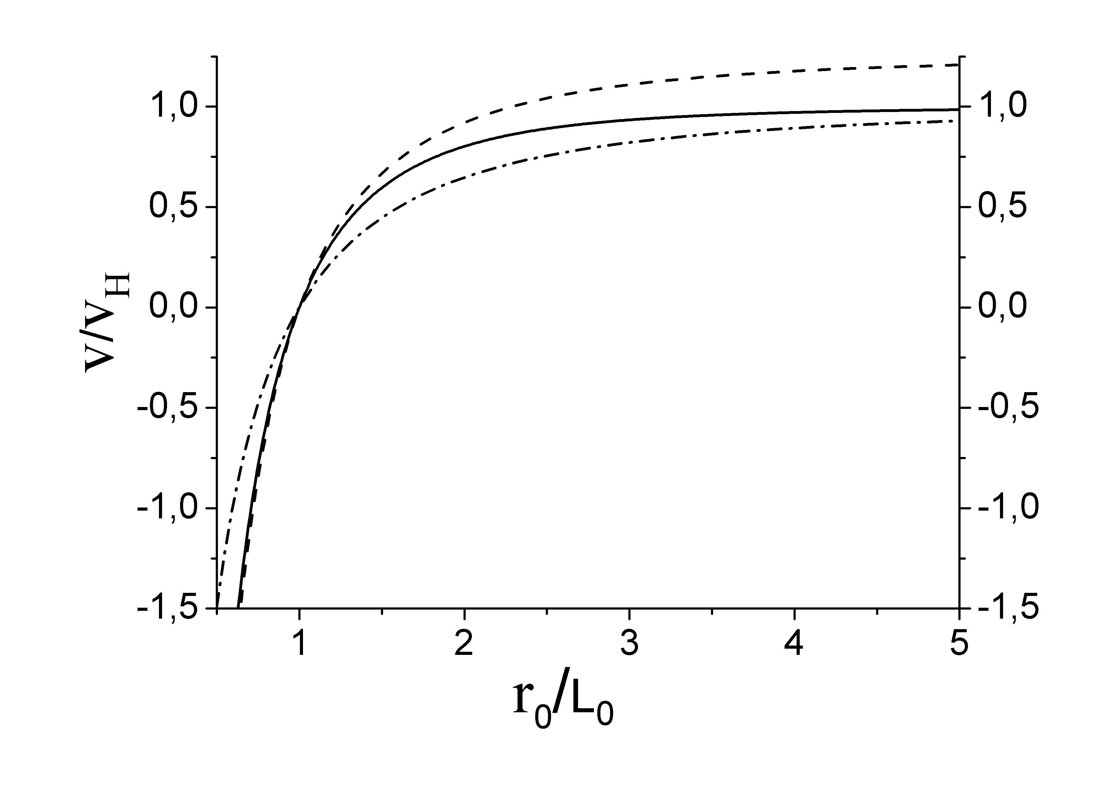
Figure 3: The speed profiles of the Hubble stream around the cluster for the point model (17) (solid line), halo model (18) (dash-dot line), and empty model (19) (dot line), respectively, represented in the natural coordinates $r_{0}/L_{0}$ and $v/v_{H}\equiv v/(r_{0}H_{0})$ (see the last paragraph in section IV).

V An example of application

In order to illustrate the solution that we have obtained, let us calculate the velocity field for several toy models of the galaxy clusters. We accept the Hubble constant value $H_{0}=73$ km/(s Mpc). In order to compare the velocity profiles for different parameters, we set all the models so that they have the same stop radius $L_{0}=1$ Mpc, which roughly corresponds to the Local Group value $L_{0}\simeq 0.9$ Mpc Karachentsev et al. (2009). As we could see in the previous paragraph, the velocity profile for a different $L_{0}$ may be found by a simple rescaling. As a good illustration of this self-similarity of the task, Baushev (2019) found that the average matter overdensity inside $L_{0}$, $\Sigma_{M,0}(L_{0})$ depends only on $\Omega_{M,0}$, and does not depend on the cluster size. In particular, $\Sigma_{M,0}(L_{0})=(3\pi/4)^{2}$ for $\Omega_{M,0}=1$ and $\Sigma_{M,0}(L_{0})\simeq 3.67$ for $\Omega_{M,0}=0.306$, which is the value measured for our Universe Tanabashi et al. (2018). Since $L_{0}$ is the same for all the models, the matter mass inside $L_{0}$ is also equal. By mass and density we mean only the matter mass and density everywhere in this section. We suppose that the dark energy always has the uniform density distribution $\Omega_{\Lambda,0}\rho_{c,0}$.

We consider three toy models of the density profile of the cluster. First, the point model, where the cluster has a central point mass $M_{c}$ and surrounded by relatively small constant density $\rho_{M}=\Omega_{M,0}\rho_{c,0}$ (which is equal to the average matter density in the Universe). The halo model also has two components: the uniform distribution of matter with the density $\Omega_{M,0}\rho_{c,0}$ and a large halo with $\rho\propto r^{-2}$, the factor being chosen so that $L_{0}=1$ Mpc. The empty model supposes that all the matter is concentrated in the cluster center, and the space around is empty (i.e., contains only dark energy). Contrary to the first two models, the empty one has incorrect asymptotic behavior: it does not transform into the undisturb Universe at large distances, and its average density tends to $\Omega_{\Lambda,0}\rho_{c,0}$, and not to $\rho_{c,0}$, as $r_{0}\to\infty$.

The matter distributions $\Sigma_{M,0}(r_{0})$ (calculated from $M_{M}(r_{0})$ with the help of equation (3)) for all three models are the following:

$$\!\Sigma_{M,0}(r_{0})\! = \!(\Sigma_{M,0}(L_{0})-\Omega_{M,0})\left(L_{0}/r_{0}\right)^{3}+\Omega_{M,0}$$ (17)

$$\!\Sigma_{M,0}(r_{0})\! = \!(\Sigma_{M,0}(L_{0})-\Omega_{M,0})\left(L_{0}/r_{0}\right)^{2}+\Omega_{M,0}$$ (18)

$$\!\Sigma_{M,0}(r_{0})\! = \!\Sigma_{M,0}(L_{0})\left(L_{0}/r_{0}\right)^{3}$$ (19)

The velocity distributions are calculated with the help of equations (10) and (14) and presented in Figures 1 and 2 for the point model (17) (solid line), halo model (18) (dash-dot line), and empty model (19) (dot line), respectively. One may see that the difference between the curves is rather significant at $r_{0}\sim 3$ Mpc, though the difference between the point and empty models is not that drastic: the density $\rho_{M}=\Omega_{M,0}\rho_{c,0}$ of the flat component of the former model is more than ten times lower than the average matter density $\sigma_{M,0}(L_{0})\simeq 3.67\rho_{c,0}$ inside $L_{0}=1$ Mpc. It suggests that the matter density profile near $L_{0}$ may in principle be restored from the Hubble stream observations of a galaxy cluster.

Finally, Figure 3 represents the velocity profiles for the three models in the natural coordinates $r_{0}/L_{0}$ and $v/v_{H}\equiv v/(r_{0}H_{0})$ (see the last paragraph in section IV for details). One can see in Figures 2 and 3 that the velocity profiles corresponding to the point and halo models converge to the undisturbed Hubble stream $v\to v_{H}=r_{0}H_{0}$ at large radii, while the profile of the empty model goes significantly higher, and the ratio $v/v_{H}$ tends to a limit significantly larger than $1$ in this case. It is not surprising: as we have already mentioned, asymptotically both point and halo models transform into the undisturb Universe. On the other hand, the empty model lacks the matter, and the uncompensated effective repulsion induced by the dark energy accelerates the Hubble expansion. The influence of the central object becomes negligible at large distances, and the empty model transforms into an empty Friedmann’s ’universe’ filled only with the dark energy, which is apparently characterized by a new Hubble constant higher than $H_{0}$. Of course, the empty model cannot be valid at large distances in reality.

To conclude, let us note that all the preceding consideration may be easily generalized to the case when the redshift $z$ of the galaxy cluster is not zero. It is enough just to find the matter fraction $\Omega_{M,z}$ and the Hubble constant $H_{z}$ at the moment $z$, and use these values instead of $\Omega_{M,0}$ and $H_{0}$, since the choice of the ’present moment’ was arbitrary in our calculations. Since $(z+1)=r_{0}/r$, we obtain from (2)

$$H^{2}_{z}=H^{2}_{0}\left(\Omega_{M,0}(z+1)^{3}+\Omega_{\Lambda,0}\right)$$

$$\Omega_{M,z}=\dfrac{\Omega_{M,0}(z+1)^{3}}{\Omega_{M,0}(z+1)^{3}+\Omega_{\Lambda,0}}.$$ (20)

For instance, if $z\gg 1$, we may neglect the dark energy (i.e., accept $\Omega_{M,0}=1$). Then the velocity profile may be found from the equations derived in the Appendix.

We would like to thank the Heisenberg-Landau Program, BLTP JINR, for the financial support of this work. This research is supported by the Munich Institute for Astro- and Particle Physics (MIAPP) of the DFG cluster of excellence ”Origin and Structure of the Universe”.

Appendix A The pure matter case ($\Omega_{\Lambda,0}=0$)

Deriving equation (7) from (5), we assume that $\Omega_{\Lambda,0}\neq 0$ and divide by it. As a result, $\alpha$ and $U$ tend to infinity as $\Omega_{\Lambda,0}\to 0$. Thus, the important instance of $\Omega_{\Lambda,0}=0$ (i.e., $\Omega_{M,0}=1$) should be considered separately. Of course, this case does not correspond to the modern Universe, but if the cluster has $z\gg 1$, we may neglect the dark energy. If $\Omega_{\Lambda,0}=0$, equation (5) can be rewritten as

$$\left(\dfrac{dx}{dt}\right)^{2}=H^{2}_{0}\left[\Sigma_{M,0}\left(\frac{1}{x}-1\right)+\left(\frac{v}{r_{0}H_{0}}\right)^{2}\right].$$ (21)

We may introduce a new quantity $w(r_{0})=1-\dfrac{v^{2}_{0}}{r^{2}_{0}H^{2}_{0}\Sigma_{M,0}}$. Since we consider an overdensity, $\Sigma_{M,0}\geq 1$, $v\leq r_{0}H_{0}$, and therefore $w\in[0;1]$. We may rewrite the equation of motion (21) as

$$H_{0}\sqrt{\Sigma_{M,0}}dt=\dfrac{\sqrt{x}dx}{\sqrt{1-wx}}.$$ (22)

As in the general case, the maximum expansion $x_{max}=r_{max}/r_{0}$ corresponds to the moment when the radicand in (22) turns to zero, i.e., $x_{max}=1/w$. Now we may exactly follow the derivation of equations (10) and (14), integrating (22). If $v\geq 0$, we integrate (22) from $x=0$ to $x=1$:

$$H_{0}t_{0}\sqrt{\Sigma_{M,0}}=\dfrac{\arcsin\left(\sqrt{w}\right)-\sqrt{w(1-w)}}{w^{3/2}}.$$ (23)

If $\Omega_{M,0}=1$, the Universe age $t_{0}$ is bound with the Hubble constant by simple relation $H_{0}t_{0}=2/3$ Zeldovich and Novikov (1983). We obtain

$$\frac{2}{3}\sqrt{\Sigma_{M,0}}=\dfrac{\arcsin\left(\sqrt{w}\right)-\sqrt{w(1-w)}}{w^{3/2}},\quad\text{if }v\geq 0.$$ (24)

If $v<0$, we integrate (22) from $x=0$ to $x_{max}=1/w$, and then from $x_{max}$ to $x=1$. After some trivial calculations, we obtain

$$\frac{2}{3}\sqrt{\Sigma_{M,0}}=\dfrac{\pi-\arcsin\left(\sqrt{w}\right)+\sqrt{w(1-w)}}{w^{3/2}},\quad\text{if }v<0.$$ (25)

Equations (24) and (25) define $v$ as an implicit function of $r_{0}$ and $\Sigma_{M,0}(r_{0})$.

References

- Karachentsev et al. (2009) I. D. Karachentsev, O. G. Kashibadze, D. I. Makarov, and R. B. Tully, MNRAS 393, 1265 (2009), eprint 0811.4610.
- Olson and Silk (1979) D. W. Olson and J. Silk, Astrophys. J. 233, 395 (1979).
- Lynden-Bell (1981) D. Lynden-Bell, The Observatory 101, 111 (1981).
- Giraud (1986) E. Giraud, A&A 170, 1 (1986).
- Peirani and de Freitas Pacheco (2008) S. Peirani and J. A. de Freitas Pacheco, A&A 488, 845 (2008), eprint 0806.4245.
- Hanski et al. (2001) M. O. Hanski, G. Theureau, T. Ekholm, and P. Teerikorpi, A&A 378, 345 (2001), eprint astro-ph/0109080.
- Peñarrubia et al. (2014) J. Peñarrubia, Y.-Z. Ma, M. G. Walker, and A. McConnachie, MNRAS 443, 2204 (2014), eprint 1405.0306.
- Baushev et al. (2017) A. N. Baushev, L. del Valle, L. E. Campusano, A. Escala, R. R. Muñoz, and G. A. Palma, JCAP 2017, 042 (2017), eprint 1606.02835.
- Baushev and Barkov (2018) A. N. Baushev and M. V. Barkov, JCAP 2018, 034, eprint 1705.05302.
- Baushev and Pilipenko (2020) A. N. Baushev and S. V. Pilipenko, Physics of the Dark Universe 30, 100679 (2020), eprint 1808.03088.
- Baushev (2019) A. N. Baushev, MNRAS 490, L38 (2019), eprint 1907.08716.
- Tanabashi et al. (2018) M. Tanabashi, K. Hagiwara, K. Hikasa, K. Nakamura, Y. Sumino, F. Takahashi, J. Tanaka, K. Agashe, G. Aielli, C. Amsler, et al., Phys. Rev. D 98, 030001 (2018).
- Gorbunov and Rubakov (2011) D. S. Gorbunov and V. A. Rubakov, Introduction to the Theory of the Early Universe: Hot Big Bang Theory (World Scientific Publishing Co, 2011).
- Zeldovich and Novikov (1983) I. B. Zeldovich and I. D. Novikov, Relativistic astrophysics. Vol.2: The structure and evolution of the universe (1983).
- Tolman (1934) R. C. Tolman, Proceedings of the National Academy of Science 20, 169 (1934).