Threshold of Primordial Black Hole Formation in Nonspherical Collapse

Abstract

We perform (3+1)-dimensional simulations of primordial black hole (PBH) formation starting from the spheroidal super-horizon perturbations. We investigate how the ellipticity (prolateness or oblateness) affects the threshold of PBH formation in terms of the peak amplitude of curvature perturbation. We find that, in the case of the radiation-dominated universe, the effect of ellipticity on the threshold is negligibly small for the large amplitude of perturbations expected for PBH formation.

I Introduction

The primordial black hole (PBH) is a generic term used to refer to black holes which are generated in the early universe and are not the final products of the stellar evolution in late times. The possibility of PBH was firstly reported in Refs. 1967SvA….10..602Z ; Hawking:1971ei , and the remarkable characteristic is that, in contrast to black holes from stellar collapse, any mass of PBH is theoretically allowed in principle. The observational constraints are actively discussed and given in a broad mass range (see e.g. Ref. Carr:2020gox for recent constraints). Despite the efforts to make constraints on the PBH abundance, PBHs are still viable and attractive candidates for a major part of dark matter (e.g., see Ref. Carr:2020gox and references therein) or the origin of the binary black holes observed by gravitational waves Abbott:2016blz ; Sasaki:2016jop . The most conventional scenario, which we suppose throughout this letter, is that PBHs are formed during the radiation-dominated universe as a result of gravitational collapse of large amplitude of cosmological perturbations generated in the inflationary era.

When one estimates the PBH abundance, at least two ingredients are needed: one is the probability distribution for the parameters characterizing the initial inhomogeneity, and the other is the criterion for PBH formation. The criterion is often set for the amplitude of the initial inhomogeneity by using a threshold value estimated through analytic Carr:1975qj ; Harada:2013epa or numerical works 1978SvA….22..129N ; 1980SvA….24..147N ; Shibata:1999zs ; Niemeyer:1999ak ; Musco:2004ak with spherical symmetry. Our aim in this letter is to estimate the effect of ellipticity on the threshold.

Recently, the spin of PBH has been attracting much attention Chiba:2017rvs ; Harada:2017fjm ; DeLuca:2019buf ; Mirbabayi:2019uph ; Fernandez:2019kyb ; He:2019cdb . Once the typical value of the PBH spin is known, it can be compared with the observed spins of black holes such as black hole binaries observed by gravitational waves Abbott:2016blz . In order to clarify the spin distribution of PBHs, eventually, we need to perform full numerical simulations starting from relevant initial settings for PBH formation. In this letter, as a first step before discussing the spin, we perform the simulation of PBH formation with radiation fluid starting from a superhorizon-scale spheroidal inhomogeneity.

Throughout this letter, we use the geometrized units in which both the speed of light and Newton’s gravitational constant are unity, $c=G=1$.

II Initial data setting

In order to describe the initial superhorizon-scale inhomogeneity, we consider the situation $\epsilon:=k/(aH_{\rm b})\ll 1$, where $1/k$ gives the characteristic comoving scale of the inhomogeneity, and $a$ and $H_{\rm b}$ are the scale factor and Hubble expansion rate in the reference universe, respectively. Then the long-wavelength growing-mode solutions of all physical quantities up to the next leading order with respect to $\epsilon$ can be derived once the leading term of the curvature perturbation $\zeta$ is given as a function of the spatial coordinates $x^{i}$ Shibata:1999zs ; Harada:2015yda . The spatial metric is given by the reference flat metric multiplied by ${\rm e}^{-2\zeta}a^{2}$ at the leading order. We use those long-wavelength solutions for the initial data in the numerical simulation.

For concreteness, let us assume that the curvature perturbation $\zeta$ is a random Gaussian variable, and consider the probability distribution of the parameters characterizing the spatial profile of the curvature perturbation based on peak theory 1986ApJ…304…15B ; Yoo:2018kvb . First, we focus on a peak in $-\zeta$, and the Taylor-series expansion up to the second order around this peak is given as follows:

$$\zeta(X^{i})=\zeta_{0}+\frac{1}{2}(\lambda_{1}X^{2}+\lambda_{2}Y^{2}+\lambda_{3}Z^{2}),$$ (1)

where $X^{i}=(X,Y,Z)$ are the appropriately rotated Cartesian coordinates. We can set $\lambda_{1}\geq\lambda_{2}\geq\lambda_{3}\geq 0$ without loss of generality. Following Refs. 1986ApJ…304…15B ; Yoo:2018kvb , we introduce the following variables:

$$\nu = -\zeta_{0}/\sigma_{0},$$ (2)

$$\xi_{1} = (\lambda_{1}+\lambda_{2}+\lambda_{3})/\sigma_{2},$$ (3)

$$\xi_{2} = (\lambda_{1}-\lambda_{3})/(2\sigma_{2}),$$ (4)

$$\xi_{3} = (\lambda_{1}-2\lambda_{2}+\lambda_{3})/(2\sigma_{2}),$$ (5)

where $\xi_{2}\geq\xi_{3}\geq-\xi_{2}$ and $\xi_{2}\geq 0$ with $\sigma_{n}$ being the $n$th-order gradient moment 1986ApJ…304…15B . Throughout this letter, we assume $\sigma_{n}/k^{n}\ll 1$. The probability density for these variables is given by 1986ApJ…304…15B ; Yoo:2018kvb

$$P(\nu,\bm{\xi})\mathrm{d}\nu\mathrm{d}\bm{\xi}=P_{1}(\nu,\xi_{1})P_{2}(\xi_{2},\xi_{3})\mathrm{d}\nu\mathrm{d}\bm{\xi},$$ (6)

where

$$P_{1}(\nu,\xi_{1})=\frac{1}{2\pi}\frac{1}{1-\gamma^{2}}\exp\left[-\frac{1}{2}\left(\nu^{2}+\frac{(\xi_{1}-\gamma\nu)^{2}}{1-\gamma^{2}}\right)\right],~{}~{}~{}~{}~{}$$ (7)

$$P_{2}(\xi_{2},\xi_{3})=\frac{5^{5/2}3^{2}}{\sqrt{2\pi}}\xi_{2}\left(\xi_{2}^{2}-\xi_{3}^{2}\right)\exp\left[-\frac{5}{2}\left(3\xi_{2}^{2}+\xi_{3}^{2}\right)\right]~{}~{}~{}~{}~{}$$ (8)

with $\gamma=\sigma_{1}^{2}/(\sigma_{0}\sigma_{2})$. From this probability density, we find that there is no correlation between the two pairs $(\nu,\xi_{1})$ and $(\xi_{2},\xi_{3})$, and the typical values for $\xi_{2}$ and $\xi_{3}$, which characterize the ellipticity, are of the order of 1.

The dimensionless quantities which purely quantify the shape of the profile can be given by

$$\chi_{1}:=\xi_{2}/\xi_{1},~{}\chi_{2}:=\xi_{3}/\xi_{1}.$$ (9)

We note that, for the high-amplitude peaks which are relevant to PBH formation, according to Eq. (7), typically we have

$$\xi_{1}\sim\nu=-\zeta_{0}/\sigma_{0}\gg 1,$$ (10)

where we have assumed $\gamma\sim 1$ and $|\zeta_{0}|\sim 1$. Therefore the typical values of $\chi_{1}$ and $\chi_{2}$ for PBH formation are much smaller than 1, that is, the initial configuration of the system is typically highly spherically symmetric. Hence, from a cosmological point of view, our main concern is in PBH formation with small ellipticity.

Because of the reflection symmetries of the profile (1) with respect to the surfaces $X^{i}=0$, we can restrict the numerical region to the cubic region $0\leq X^{i}\leq L$ ($i=1,2,3$) as is adopted in Refs. Yoo:2013yea ; Yoo:2018pda . Here we consider the following specific curvature perturbation profile characterized by 4 parameters $\mu$ and $k_{i}$:

$$\zeta=-\mu\exp\left[-\frac{1}{2}\left(k_{1}^{2}X^{2}+k_{2}^{2}Y^{2}+k_{3}^{2}Z^{2}\right)\right]W(R),$$ (11)

where $R=X^{2}+Y^{2}+Z^{2}$ and the function $W(R)$, which we do not specify here (see Eq. (24) in Ref. Yoo:2018pda ), is introduced to smooth out the tail of the Gaussian profile on the boundary of the cubic region.

In the simulation, we fix the square sum $\hat{\xi}_{1}$ of the wave numbers $k^{i}$ to $k^{2}$ as follows:

$$\hat{\xi}_{1}:=\xi_{1}\sigma_{2}/\mu=k_{1}^{2}+k_{2}^{2}+k_{3}^{2}=k^{2},$$ (12)

where we have used the relation $\mu=-\zeta_{0}$. Defining $\hat{\xi}_{2}:=\xi_{2}\sigma_{2}/\mu$ and $\hat{\xi}_{3}:=\xi_{3}\sigma_{2}/\mu$, we find $\chi_{1}=\hat{\xi}_{2}/k^{2}$ and $\chi_{2}=\hat{\xi}_{3}/k^{2}$, so that

$$3k_{1}^{2} = (\hat{\xi}_{1}+3\hat{\xi}_{2}+\hat{\xi}_{3})=k^{2}(1+3\chi_{1}+\chi_{2}),$$ (13)

$$3k_{2}^{2} = (\hat{\xi}_{1}-2\hat{\xi}_{3})=k^{2}(1-2\chi_{2}),$$ (14)

$$3k_{3}^{2} = (\hat{\xi}_{1}-3\hat{\xi}_{2}+\hat{\xi}_{3})=k^{2}(1-3\chi_{1}+\chi_{2}).$$ (15)

Let us summarize the physical parameters characterizing the initial data. First, we set the initial scale factor to 1. Taking $L$ as the unit of the length scale, we set $1/k=L/10$. The initial time slice is chosen so that it has a constant mean curvature $K_{0}$ by using the gauge degree of freedom. Then the initial Hubble parameter $H_{0}:=-K_{0}/3$ is chosen so that $1/H_{0}=L/50=1/(5k)$, namely the scale of the inhomogeneity $1/k$ is 5 times larger than the initial Hubble length $1/H_{0}$. In this letter, we focus on the spheroidal profiles of the curvature perturbation, which are given by $\chi_{1}=|\chi_{2}|$. Then finally we have two free parameters $\mu$ and $\chi_{2}$. The positive (negative) value of $\chi_{2}$ stands for oblateness (prolateness). In Fig. 1, we show the fluid comoving density at the initial time for $\mu=0.8$ and $\chi_{2}=0.1$.

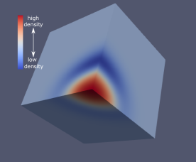
Figure 1: The fluid comoving density at the initial time for $\mu=0.8$ and $\chi_{2}=0.1$.

III Numerical schemes

For the simulation we use the 4th-order Runge-Kutta method with the BSSN (Baumgarte-Shapiro-Shibata-Nakamura) formalism Shibata:1995we ; Baumgarte:1998te with the same gauge condition as in Ref. Yoo:2013yea and a central scheme with MUSCL (Mono Upstream-centered Scheme for Conservation Laws) 2000JCoPh.160..241K ; Shibata:2005jv method for the fluid dynamics. Since we are interested in a cosmological setting, the boundary condition cannot be asymptotically flat. If spherical symmetry is imposed, we may use the asymptotic Friedmann-Lemaître-Robertson-Walker (FLRW) condition Shibata:1999zs or just cut out the outer region causally connected to the outer boundary taking a sufficiently large initial region. However, the validity of the asymptotic FLRW condition is not clear in general, and the cutting-out procedure is not available due to the limited computational resources. Therefore we adopt the periodic boundary condition as is imposed in Refs. Yoo:2013yea ; Yoo:2018pda . In this setting, we need to simultaneously resolve the scales of the gravitational collapse and cosmological expansion. In order to overcome this difficulty, for the spatial coordinates, we use the scale-up coordinates introduced in Ref. Yoo:2018pda with the parameter $\eta=15$, where the ratio between the Cartesian coordinate lengths of the unit coordinate interval at the boundary and origin is $1+2\eta$. In the initial stage of the evolution, the typical time scale should be given by $1/|K|$ with $K$ being the trace of the extrinsic curvature at the point $x=y=z=L$. Thus we fix the time interval $\Delta t$ of the simulation by

$$\Delta t=C\times\min\left\{\Delta x,1/(10|K|)\right\},$$ (16)

where we set the spatial grid interval $\Delta x=1/100$ and $C=1/20$.

IV Results

IV.1 Spherical initial data

For the spherically symmetric cases, we find that the threshold value $\mu_{\rm th}$ is around 0.8. For $\mu\leq 0.795$, the collapse stops and bounces back. We can check this behavior from the time evolution of the value of the lapse function at the origin (Fig. 2).

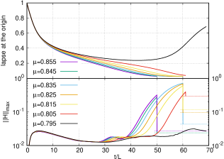
Figure 2: The value of the lapse function at the origin (upper) and the max norm of the Hamiltonian constraint (lower) as functions of the time for each parameter set.

On the other hand, for $\mu\geq 0.805$, the fluid does not bounce back and finally we find an apparent horizon in the center (Fig. 3).

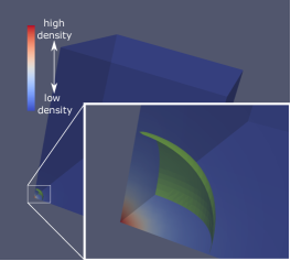
Figure 3: Apparent horizon and the fluid comoving density at the time of the horizon formation for $\mu=0.805$.

We also show the time evolution of the max norm of the Hamiltonian constraint violation $||H||_{\rm max}$ in Fig. 2. The function $||H||$ is normalized so that $||H||\leq 1$ at each grid point. We take a maximum over the whole computing region as $||H||_{{\rm max}}$ before the horizon formation, while we switch from the whole region to outside the horizon after the horizon formation. This switch gives a discontinuous reduction in $||H||_{{\rm max}}$ as seen in the lower panel of Fig. 2 because $||H||$ takes a maximum in the very central region before the horizon formation and the central region gets hidden behind the horizon after the horizon formation. If the value of $||H||_{\rm max}$ after the discontinuous reduction, which is denoted by the horizontal dashed line in the lower panel of Fig. 2, is well controlled, we can regard the computation outside the horizon acceptable. Fig. 2 shows that even after the reduction, the constraint is significantly violated ($||H||_{\rm max}\sim 0.4$) around the horizon for the $\mu=0.805$ case. For $\mu\geq 0.845$, however, we find that $||H||_{\rm max}$ is well suppressed outside the apparent horizon at the time when we detect the horizon. For $0.805\lesssim\mu\lesssim 0.845$, we need more effort to resolve the horizon formation. On the other hand, since $||H||_{\rm max}$ is always well controlled ($\lesssim 0.03$) for the bouncing dynamics for $\mu=0.795$, we expect that the threshold value is given by $\mu_{\rm th}\simeq 0.8$.

Since the system is spherical if we ignore the effect of the boundary condition, we can check the resultant threshold value based on the compaction function $\mathcal{C}$ in the constant mean curvature slice Shibata:1999zs , which is directly related to the more conventional indicator $\bar{\delta}$, the averaged density perturbation in the overdense region on the comoving slicing at horizon entry, through $\bar{\delta}=(4/3)\mathcal{C}$ if the radius for $\mathcal{C}$ is identified with that of $\bar{\delta}$ Harada:2015yda . The threshold value $\sim 0.4$ of the maximum value $\mathcal{C}_{\rm max}$ is conventionally used. More recently, it has been reported that the volume average $\bar{\mathcal{C}}$ of $\mathcal{C}$ within the radius $r_{\rm m}$, at which $\mathcal{C}$ takes a maximum, gives a very stable threshold value of 0.3 at a level of a few % accuracy for a moderate shape of the inhomogeneity Escriva:2019phb . In Fig. 4, we show the values of $\bar{\mathcal{C}}$, ${\mathcal{C}}_{\rm max}$ and $\bar{\delta}$ as functions of $\mu$.

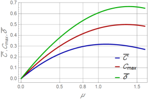
Figure 4: The averaged compaction function $\bar{\mathcal{C}}$, the maximum compaction function ${\mathcal{C}}_{\rm max}$ and the averaged comoving density perturbation $\bar{\delta}$ in the overdense region at horizon entry as functions of $\mu$.

For $\mu=0.8$, in our initial setting, the value of $\bar{\mathcal{C}}$ is given by 0.297 which is about only 1% deviation from the reference value 0.3. Having this agreement, throughout this letter, we conclude that a PBH is formed if the bouncing-back behavior is not observed. For all the non-bouncing cases, even if the value of $||H||_{\rm max}$ becomes of the order of 1, we can eventually find an apparent horizon.

IV.2 Non-spherical initial data

By numerical simulations with nonzero $\chi_{2}$, we find that the PBH formation becomes harder for larger ellipticity, which is consistent with the hoop conjecture 1972mwm..book…..K . We look for the critical value of $\chi_{2}$ beyond or below which no horizon is formed, for $\mu=0.805$. As a result, we find PBH formation for $-0.06\leq\chi_{2}\leq 0.08$ with $\mu=0.805$, while we find a bouncing behavior for $\chi_{2}\leq-0.07$ or $\chi_{2}\geq 0.09$ (see Fig. 5). Although we find a bouncing behavior for $\chi_{2}=-0.07$, since the value of $\chi_{2}$ is very close to the critical value, the Hamiltonian constraint is significantly violated near the center similarly to the collapsing cases. Unless $-0.08<\chi_{2}<0.09$, the constraint violation is well suppressed.

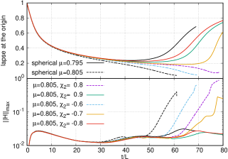
Figure 5: The value of the lapse function at the origin (upper) and the max norm of the Hamiltonian constraint (lower) as functions of the time for each parameter set. The dashed lines are corresponding to the cases with horizon formation.

In Figs. 6 and 7, we show the time evolution of the comoving fluid density on each axis for $\chi_{2}=0.08$ and $0.09$ cases, respectively.

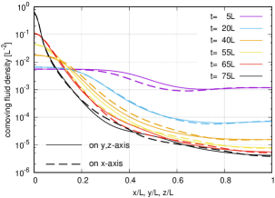
Figure 6: Time evolution of the comoving fluid density on each axis for $\chi_{2}=0.08$.

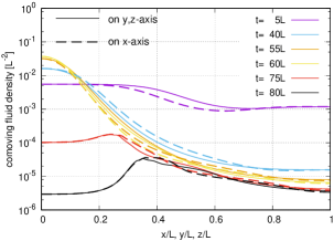
Figure 7: Time evolution of the comoving fluid density on each axis for $\chi_{2}=0.09$.

For both cases, in late times, the configuration is highly spherically symmetric near the center. We also find an oscillatory behavior between prolateness and oblateness, which is expected by the result of the linear analysis of the nonspherical perturbations around the spherically symmetric critical solution reported in Ref. Gundlach:1999cw . The oscillation is more apparent in Fig. 8, where the values of the comoving fluid density at specific spatial points are given as functions of the time.

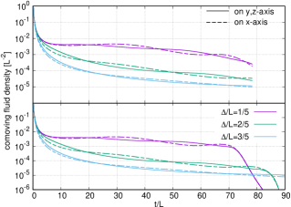
Figure 8: Time evolution of the comoving fluid density at fixed spatial points on axes for $\chi_{2}=0.08$ (upper) and $\chi_{2}=0.09$ (lower), where $\Delta$ is the coordinate distance from the origin.

Therefore we conclude that the system is stable against the non-spherically symmetric perturbation of the current setting, whereas it slightly changes the threshold value of $\mu$ for the PBH formation.

V Summary and discussion

We have performed numerical simulations for PBH formation for several values of $\chi_{2}$, which characterizes the initial spheroidal profile. It has been shown that the value of $\chi_{2}\sim 0.1$ gives only $\sim 1\%$ difference in the threshold value of the amplitude of the curvature perturbation $\mu$, and we typically have $|\chi_{2}|\ll 1$ for PBH formation in the radiation dominated universe. Thus we conclude that the effect of ellipticity on the threshold of PBH formation is highly limited and usually negligible in standard situations for PBH formation in the radiation-dominated universe.

As is expected from the general nature of the critical collapse, the final fate is sensitive to the parameters $\mu$ and $\chi_{2}$ around the critical values, so that the time evolution can be clearly classified with the existence of the bouncing behavior. Thus we can read off the threshold value and discuss the effect of the ellipticity although the resolution is not fine enough to resolve the horizon in our simulation. In order to analyze the finer structure of the solutions around the criticality, we need a finer resolution near the center. If the equation of state of the matter field is softer than the radiation fluid, the result would drastically change (see Refs. 1982SvA….26….9P ; Harada:2016mhb ; Harada:2017fjm ; Kokubu:2018fxy for the pressureless matter). In order to analyze the spin generation of PBH, we have to consider the initial setting in which the tidal torque works during the collapse DeLuca:2019buf . These are beyond the scope of this letter and are left as future issues.

- (1) Y. B. Zel’dovich and I. D. Novikov, Soviet Ast. 10, 602 (1967).
- (2) S. Hawking, Mon. Not. Roy. Astron. Soc. 152, 75 (1971).
- (3) B. Carr, K. Kohri, Y. Sendouda, and J. Yokoyama, (2020), arXiv:2002.12778.
- (4) Virgo, LIGO Scientific, B. P. Abbott et al., Phys. Rev. Lett. 116, 061102 (2016), arXiv:1602.03837.
- (5) M. Sasaki, T. Suyama, T. Tanaka, and S. Yokoyama, Phys. Rev. Lett. 117, 061101 (2016), arXiv:1603.08338.
- (6) B. J. Carr, Astrophys. J. 201, 1 (1975).
- (7) T. Harada, C.-M. Yoo, and K. Kohri, Phys. Rev. D88, 084051 (2013), arXiv:1309.4201, [Erratum: Phys. Rev.D89,no.2,029903(2014)].
- (8) D. K. Nadezhin, I. D. Novikov, and A. G. Polnarev, Soviet Ast. 22, 129 (1978).
- (9) I. D. Novikov and A. G. Polnarev, Soviet Ast. 24, 147 (1980).
- (10) M. Shibata and M. Sasaki, Phys. Rev. D60, 084002 (1999), arXiv:gr-qc/9905064.
- (11) J. C. Niemeyer and K. Jedamzik, Phys. Rev. D59, 124013 (1999), arXiv:astro-ph/9901292.
- (12) I. Musco, J. C. Miller, and L. Rezzolla, Class. Quant. Grav. 22, 1405 (2005), arXiv:gr-qc/0412063.
- (13) J. D. Barrow and J. Silk, Astrophys. J. 250, 432 (1981).
- (14) F. Kühnel and M. Sandstad, Phys. Rev. D94, 063514 (2016), arXiv:1602.04815.
- (15) T. Chiba and S. Yokoyama, PTEP 2017, 083E01 (2017), arXiv:1704.06573.
- (16) T. Harada, C.-M. Yoo, K. Kohri, and K.-I. Nakao, Phys. Rev. D96, 083517 (2017), arXiv:1707.03595, [Erratum: Phys. Rev.D99,no.6,069904(2019)].
- (17) V. De Luca, V. Desjacques, G. Franciolini, A. Malhotra, and A. Riotto, JCAP 1905, 018 (2019), arXiv:1903.01179.
- (18) M. Mirbabayi, A. Gruzinov, and J. Noreña, (2019), arXiv:1901.05963.
- (19) N. Fernandez and S. Profumo, JCAP 1908, 022 (2019), arXiv:1905.13019.
- (20) M. He and T. Suyama, Phys. Rev. D100, 063520 (2019), arXiv:1906.10987.
- (21) T. Harada, C.-M. Yoo, T. Nakama, and Y. Koga, Phys. Rev. D91, 084057 (2015), arXiv:1503.03934.
- (22) D. H. Lyth, K. A. Malik, and M. Sasaki, JCAP 0505, 004 (2005), arXiv:astro-ph/0411220.
- (23) J. M. Bardeen, J. R. Bond, N. Kaiser, and A. S. Szalay, Astrophys. J. 304, 15 (1986).
- (24) C.-M. Yoo, T. Harada, J. Garriga, and K. Kohri, (2018), arXiv:1805.03946.
- (25) C.-M. Yoo, H. Okawa, and K.-i. Nakao, Phys. Rev. Lett. 111, 161102 (2013), arXiv:1306.1389.
- (26) C.-M. Yoo, T. Ikeda, and H. Okawa, Class. Quant. Grav. 36, 075004 (2019), arXiv:1811.00762.
- (27) M. Shibata and T. Nakamura, Phys.Rev. D52, 5428 (1995).
- (28) T. W. Baumgarte and S. L. Shapiro, Phys.Rev. D59, 024007 (1999), arXiv:gr-qc/9810065.
- (29) A. Kurganov and E. Tadmor, Journal of Computational Physics 160, 241 (2000).
- (30) M. Shibata and J. A. Font, Phys. Rev. D72, 047501 (2005), arXiv:gr-qc/0507099.
- (31) A. Escrivà, C. Germani, and R. K. Sheth, Phys. Rev. D101, 044022 (2020), arXiv:1907.13311.
- (32) K. S. Thorne, Magic Without Magic , (1972), John Archibald Wheeler, John R. Klauder(eds.), Freeman, San Fransisco.
- (33) C. Gundlach, Phys. Rev. D65, 084021 (2002), arXiv:gr-qc/9906124.
- (34) A. G. Polnarev and M. Y. Khlopov, Soviet Ast. 26, 9 (1982).
- (35) T. Harada, C.-M. Yoo, K. Kohri, K.-i. Nakao, and S. Jhingan, Astrophys. J. 833, 61 (2016), arXiv:1609.01588.
- (36) T. Kokubu, K. Kyutoku, K. Kohri, and T. Harada, Phys. Rev. D98, 123024 (2018), arXiv:1810.03490.