On the Feedback Law in Stochastic Optimal Nonlinear Control

Abstract

We consider the problem of nonlinear stochastic optimal control. This problem is thought to be fundamentally intractable owing to Bellman’s “curse of dimensionality”. We present a result that shows that repeatedly solving an open-loop deterministic problem from the current state with progressively shorter horizons, similar to Model Predictive Control (MPC), results in a feedback policy that is $O(\epsilon^{4})$ near to the true global stochastic optimal policy. We show that the optimal deterministic feedback problem has a perturbation structure in that higher-order terms of the feedback law do not affect lower-order terms, and that this structure is lost in the optimal stochastic feedback problem. Consequently, solving the Stochastic Dynamic Programming (DP) problem is highly susceptible to noise, even when tractable, and in practice, the MPC-type feedback law offers superior performance even for stochastic systems.

I INTRODUCTION

In this paper, we consider the problem of finite time nonlinear stochastic optimal control, specifically the stochastic dynamic system:

$$dx=(f(x)+g(x)u)dt+\epsilon dw,$$

where $w$ is a Wiener process, and the cost to be optimized is $J^{\pi}=\mathop{\mathbb{E}}_{\begin{subarray}{c}{}\end{subarray}}\left[{\int_{0}^{T}c(x_{t},\pi_{t}(x_{t}))dt+c_{T}(x_{T})}\right]$, where the incremental cost has the form $c(x,u)=l(x)+\frac{1}{2}u^{\prime}Ru$, $\pi_{t}(x_{t})$ is a control policy and the cost is minimized over all possible such policies. We present a result that establishes that repeatedly solving a deterministic optimal control, or open-loop problem, from the current state, shown to be equivalent to applying the deterministic feedback policy to the system, results in a feedback policy that is $O(\epsilon^{4})$ near-optimal to the optimal stochastic feedback policy, in terms of the small noise parameter $\epsilon$. Our analysis shows that under the relatively mild conditions of affine in control dynamics and quadratic in control cost, the open-loop solution obtained by satisfying the Minimum Principle [1] is globally optimum. Further, the deterministic feedback law has a perturbation structure in the sense that the higher-order feedback terms do not affect the lower-order terms, and that this structure is lost for the optimal stochastic problem. We obtain the equations that need to be satisfied by the linear and higher-order feedback terms in the optimal feedback law. Although near-optimal, empirical evidence shows that this replanning based Model Predictive Control (MPC)-type policy is the best we can do in practice, in the sense that albeit the optimal stochastic law should, in theory, have better performance, solving the stochastic problem is highly susceptible to noise owing to its lack of the perturbation structure, and in practice, the MPC-type law gives better performance. Thus, this result resolves the trade-off between tractability and optimality in stochastic feedback control problems, showing that, in practice, “what is tractable is also optimal”. In this paper, we consider the case where an analytical model is available for the control synthesis, we consider the case of data-based control in a companion paper [2]. A final note here is that the system considered in this work is not the most general, and our goal is not to analyze the most general case, rather, we show that even in the simplest case considered here, the stochastic problem is fundamentally intractable, and the best we can do in practice is use the deterministic feedback law, which is implemented by re-planning the open-loop as necessary.

A large majority of sequential decision making problems under uncertainty can be posed as a nonlinear stochastic optimal control problem that requires the solution of an associated Dynamic Programming (DP) problem, however, as the state dimension increases, the computational complexity goes up exponentially in the state dimension [3]: the manifestation of the so-called Bellman’s “curse of dimensionality (CoD)” [4]. To understand the CoD better, consider the simpler problem of estimating the cost-to-go function of a feedback policy $\mu_{t}(\cdot)$. Let us further assume that the cost-to-go function can be “linearly parametrized” as: $J_{t}^{\mu}(x)=\sum_{i=1}^{M}\alpha^{i}_{t}\phi_{i}(x)$, where the $\phi_{i}(x)$’s are some a priori basis functions. Then the problem of estimating $J_{t}^{\mu}(x)$ becomes that of estimating the parameters $\bar{\alpha}_{t}=\{\alpha^{1}_{t},\cdots,\alpha^{M}_{t}\}$. This can be shown to be the recursive solution of the linear equations $\bar{\alpha}_{t}=\bar{c}_{t}+L_{t}\bar{\alpha}_{t+1},\text{ where }\bar{c}_{t}=[c^{i}_{t}],$ with $c^{i}_{t}=\int c(x,\mu_{t}(x))\phi_{i}(x)\,dx,$ and $L_{t}^{ij}=\int\int p^{\mu_{t}}(x^{\prime}|x)\phi_{i}(x^{\prime})\phi_{j}(x)\,dx^{\prime}\,dx,\;i,j\in\{1,\dots,M\},$ where $p^{\mu_{t}}(./.)$ is the transition density of the Markov chain under policy $\mu_{t}$. This can be done using numerical quadratures given knowledge of the model $p^{\mu}(x^{\prime}|x)$, termed Approximate DP (ADP), or alternatively, in Reinforcement Learning (RL), simulations of the process under the policy $\mu_{t}$, $x_{t}\xrightarrow{\mu_{t}(x_{t})}x_{t+1}\rightarrow\cdots$, is used to get an approximation of the $L^{ij}_{t}$ by sampling, and solve the equation above either batchwise or recursively [5, 3]. But, as the dimension $d~{}$ increases, the number of basis functions, and more importantly, the number of evaluations required to evaluate the integrals go up exponentially. There has been recent success using the Deep RL paradigm where deep neural networks are used as nonlinear function approximators to keep the parametrization tractable [6, 7, 8, 9, 10], however, the training times required for these approaches, and the variance of the solutions, is still prohibitive. Hence, the primary problem with ADP/ RL techniques is the CoD inherent in the complex representation of the cost-to-go function, and the exponentially large number of evaluations required for its estimation resulting in high solution variance which makes them unreliable and inaccurate.

In the case of continuous state, control, and observation space problems, the Model Predictive Control [11, 12] approach has been used with a lot of success in the control system and robotics community. For deterministic systems, the process results in solving the original DP problem in a recursive online fashion. However, stochastic control problems, and the control of uncertain systems in general, is still an unresolved problem in MPC. As succinctly noted in [11], the problem arises due to the fact that in stochastic control problems, the MPC optimization at every time step cannot be over deterministic control sequences, but rather has to be over feedback policies, which is, in general, difficult to accomplish since a tractable parameterization of such policies to perform the optimization over, is, in general, unavailable. Thus, the tube-based MPC approach, and its stochastic counterparts, typically consider linear systems [13, 14, 15] for which a linear parametrization of the feedback policy suffices but the methods become intractable when dealing with nonlinear systems [16]. In more recent work, event-triggered MPC [17, 18] keeps the online planning computationally efficient by triggering replanning in an event driven fashion rather than at every time step. We note that event-triggered MPC inherits the same issues mentioned above with respect to the stochastic control problem, and consequently, the techniques are intractable for nonlinear systems. There has been recent work showing the near-optimality of MPC with a perturbation analysis [19, 20, 21], but this work considers a deterministic problem setting with unknown model parameters in the system dynamics, and the regret bound provided is with respect to the controller that has perfect knowledge of the model, in contrast to the near-optimality of the deterministic feedback to the optimal stochastic law shown in this work. 

The basic issue at work above is that, albeit solving the open-loop problem via the Minimum Principle (MP) is much easier, solving for the optimal feedback control under uncertainty requires the solution of the DP equation, which is intractable. Moreover, this also begs the question, since all systems are subject to uncertainty, what is the utility of deterministic optimal control?
Contributions: In this work, we establish that the basic MPC-type approach of solving the deterministic open-loop problem (with progressively shorter horizons) at every time step results in a near-optimal policy, to $O(\epsilon^{4})$, for a nonlinear stochastic system. The result uses a perturbation expansion of the cost-to-go function in terms of a perturbation parameter $\epsilon$. We show the global optimality of the open-loop solution obtained by satisfying the Minimum Principle [1] using the classical Method of Characteristics [22] thereby establishing that the MPC feedback law is indeed the optimal deterministic feedback law. Further, we show that the deterministic feedback law has a perturbation structure that is lost in the stochastic problem. We obtain the true linear and higher order feedback gain equations of the optimal deterministic policy as a by-product, which is very different from the Riccati equation governing a typical LQR perturbation feedback design [1]. Finally, albeit the MPC law is only “near-optimum”, our empirical evidence shows that this deterministic law has better performance than the stochastic law, obtained by solving the stochastic DP problem computationally, showing the susceptibility of the stochastic DP problem to noise owing to the loss of the perturbation structure, quite apart from the usual Curse of Dimensionality. Thus, in practice, the MPC law is the best one can do. In contrast to [23], we show fourth order near-optimality to the optimal stochastic solution, the global optimality of the open-loop solution and the perturbation structure of the deterministic feedback law, without which MPC is heuristic, and analytical as well as empirical evidence regarding the superiority of MPC to stochastic DP even when the DP problem is not subject to the curse of dimensionality. The current manuscript expands on our previously published conference paper [24]. In particular, we provide detailed proofs of all our developments, explain the loss of perturbation structure in the stochastic problem, and provide a comprehensive empirical evaluation of the theory proposed in this manuscript.

The rest of the document is organized as follows: Section II states the problem, Section III presents three fundamental results that represent the three legs of the stool that supports the fact that the MPC feedback law is near-optimal, which is established in Section IV. We illustrate our results empirically in Section V using simple 1-dimensional examples for which the stochastic DP problem can be solved, and more practical examples from nonlinear robotic planning.

II PRELIMINARIES

The following outlines the finite time stochastic optimal control problem formulation, and the associated deterministic problem, along with the associated Dynamic Programming (DP) problems that we shall study in this work.

System Model

For a dynamic system, we denote the state and control vectors by $x\in\ \mathbb{X}\subset\ \mathbb{R}^{n_{x}}$ and $u\in\ \mathbb{U}\subset\ \mathbb{R}^{n_{u}}$ respectively. The dynamics of the system are governed by the stochastic differential equation (SDE):

$$dx=(f(x)+g(x)u)dt+\epsilon dw,$$ (1)

where $w$ is a Wiener process with covariance $Q$, and $\epsilon$ is a small parameter modulating the noise input to the system.

Stochastic optimal control problem

The stochastic optimal control problem for an initial state $x_{0}$ is defined as:

$$J_{\pi^{*}}(x_{0})=\min_{\Pi}\ \mathop{\mathbb{E}}_{\begin{subarray}{c}{}\end{subarray}}\left[{\int^{T}_{0}c(x_{t},\pi_{t}(x_{t}))dt+c_{T}(x_{T})}\right],$$ (2)

subject to the SDE (1), where the optimization is over a family of time-varying feedback policies $\Pi:=\{\pi_{t}(x);t\in[0,T]$}; $J_{\pi^{*}}(\cdot):\mathbb{X}\rightarrow\mathbb{R}$ is the cost function on executing the optimal policy $\pi^{*}$; $c(\cdot,\cdot):\mathbb{X}\times\mathbb{U}\rightarrow\mathbb{R}$ is the incremental cost function and we assume $c(x,u)=l(x)+\frac{1}{2}u^{\prime}Ru,R>0$; and $c_{T}(\cdot):\mathbb{X}\rightarrow\mathbb{R}$ is the terminal cost function; where $T$ is the “finite time horizon” of the problem.

II-A Stochastic Dynamic Programming (DP)

For simplicity, we consider the scalar case for the derivations below, the vector generalization is given at the end of the section. The stochastic DP equation for the optimal control problem on the system in Eq. (1), after discretizing the time by $\Delta t$, such that $T=N\Delta t$, is given by:

$$J_{k}(x)=\min_{u_{k}}\{c(x,u_{k})\Delta t+E[J_{k+1}(x^{\prime})]\},$$ (3)

where $x^{\prime}=x+f(x)\Delta t+g(x)u_{k}\Delta t+\epsilon w_{t}\sqrt{\Delta t}$ and $J_{k}(x)=J(k\Delta t,x)$ denotes the cost-to-go of the system given that it is at state $x$ at time $k\Delta t$. The above equation is marched back in time from the terminal condition $J_{N}(x)=c_{T}(x)$. Further simplification is possible as we let the discretization time $\Delta t\rightarrow 0$. To see this:

$$J_{k+1}(x^{\prime}) =J_{k+1}(x+(f(x)+g(x)u_{k})\Delta t+\epsilon w\sqrt{\Delta t}),$$

$$\approx J_{k+1}(x)+\frac{\partial J_{k+1}}{\partial x}{\Big{(}(f(x)+g(x)u_{k})\Delta t+\epsilon w\sqrt{\Delta t}\Big{)}\ }$$

$$\quad+{\frac{\epsilon^{2}}{2}\ }\frac{\partial^{2}J_{k+1}}{\partial x^{2}}w^{2}\Delta t,$$

where the $J_{k+1}$ is expanded to second order due to the $\sqrt{\Delta t}$ factor for the Wiener process. Taking expectations implies:

$$\mathop{\mathbb{E}}_{\begin{subarray}{c}{}\end{subarray}}\left[{J_{k+1}(x^{\prime})}\right] \approx J_{k+1}(x)+\frac{\partial J_{k+1}}{\partial x}(f(x)+g(x)u_{k})\Delta t$$

$$\quad+\frac{\epsilon^{2}}{2}\frac{\partial^{2}J_{k+1}}{\partial x^{2}}\Delta t,$$

where, we have assumed $\mathop{\mathbb{E}}_{\begin{subarray}{c}{}\end{subarray}}\left[{w^{2}}\right]=Q=1$, since the parameter $\epsilon$ captures its effect. Note: The noise covariance $Q$ will be assumed to be 1 in the rest of the theoretical development for simplicity, $Q$ will simply appear as a scaling factor when included, and will not affect the results we derive.

Using the above equation and substituting into (3) gives:

$$J_{k}(x) \approx\min_{u_{k}}\underbrace{[c(x,u_{k})+\frac{\partial J_{k+1}}{\partial x}(f(x)+g(x)u_{k})]}_{H(x,u_{k})}\Delta t$$

$$\quad+\frac{\epsilon^{2}}{2}\frac{\partial^{2}J_{k+1}}{\partial x^{2}}\Delta t+J_{k+1}(x).$$

Taking $J_{k+1}(x)$ to the left hand side of the above equation, dividing by $\Delta t$ and taking the limit as $\Delta t\rightarrow 0$ gives us the continuous time DP or the stochastic Hamilton-Jacobi-Bellman (HJB) equation:

$$-\frac{\partial J}{\partial t}=\min_{u}H(x,u)+\frac{\epsilon^{2}}{2}\frac{\partial^{2}J}{\partial x^{2}},$$ (4)

where $H(x,u)=c(x,u)+\frac{\partial J}{\partial x}(f(x)+g(x)u)$ is the Hamiltonian of the system, and $J=J(t,x)$ .
Let $u(t,x)$ denote the corresponding optimal policy. Suppose that $c(x,u)=l(x)+\frac{1}{2}ru^{2},~{}r>0$, i.e., the incremental cost function is quadratic in the control variable. Then, it is sufficient that the optimal control $u$ satisfies the first-order necessary condition (since the Hamiltonian $H(x,u)$ is strictly quadratic in $u$):

$$u=-\frac{1}{r}g(x)J^{x},~{}\text{where}~{}J^{x}=\frac{\partial J(t,x)}{\partial x}.$$ (5)

II-B The Deterministic Problem

Let us now consider the deterministic problem, i.e., Eq. (1) with $\epsilon=0$ and the same cost as in (2), except there is no expectation due to the lack of stochasticity. Utilizing essentially identical arguments as for the stochastic case, the optimal cost-to-go of the deterministic system, $\phi(t,x)$, satisfies the deterministic DP equation:

$$-\frac{\partial{\phi}}{\partial t}=\min_{u}H(x,u),$$ (6)

where the Hamiltonian $H(x,u)=c(x,u)+\frac{\partial\phi}{\partial x}(f(x)+g(x)u)$ is the exact same as that in the stochastic problem and the only difference is the missing diffusion term $\epsilon^{2}\frac{\partial^{2}J}{\partial x^{2}}$. Finally, identical to the stochastic case, if the incremental cost $c(x,u)$ is quadratic in the control variable, the optimal control in the deterministic case is given by: $u^{d}=-\frac{1}{r}g(x)\phi^{x}$, where $\phi^{x}=\frac{\partial\phi}{\partial x}$.

II-C Vector Generalization

The stochastic HJB equation can be written as:

$$-\frac{\partial J}{\partial t}=\min_{u}H(x,u)+\frac{\epsilon^{2}}{2}\sum_{i}\sum_{j}\frac{\partial^{2}J}{\partial x_{i}\partial x_{j}}Q_{ij},$$ (7)

where $H(x,u)=c(x,u)+\frac{\partial J}{\partial x}^{\prime}(f(x)+g(x)u)$ and $Q=[Q_{ij}]$ is the intensity of the vector Wiener process. In order to avoid the notational burden, we represent the vector state with the lowercase $x$ and the vector Wiener process with lowercase $w$. Further, if the cost function is quadratic in the control, i.e., $c(x,u)=l(x)+\frac{1}{2}u^{\prime}Ru,R>0$, the optimal control policy obtained by minimizing the Hamiltonian is:

$$u=-R^{-1}g(x)^{\prime}J^{x}.$$ (8)

The deterministic HJB equation is identical except for the lack of the second order differential terms:

$$-\frac{\partial\phi}{\partial t}=\min_{u}H(x,u),$$ (9)

where the Hamiltonian $H(x,u)$ is the same as that for the stochastic case. Further, the optimal control policy for the deterministic case is given by:

$$u^{d}=-R^{-1}g(x)^{\prime}\phi^{x},$$ (10)

assuming a quadratic in control cost.

We shall make the following assumptions in the rest of the paper, and unless otherwise stated, all results assume the following.

Assumption 1

Cost Structure. We assume that the incremental cost $c(x,u)$ is quadratic in the control variable, i.e., $c(x,u)=l(x)+\frac{1}{2}u^{\prime}Ru$, with $R$ positive definite.

Assumption 2

Smoothness. We shall also assume that all the involved functions: $f(x),g(x),l(x),c_{T}(x)$ are five times continuously differentiable ($\mathcal{C}^{5}$) in their arguments.

III A PERTURBATION ANALYSIS OF OPTIMAL FEEDBACK CONTROL

In the following four subsections, we establish four basic results that we shall use to establish the near optimality of the MPC law in Section IV. In Section III A, we characterize the performance of any given feedback policy as a perturbation (series) expansion in the parameter $\epsilon$. We establish that the $O(\epsilon^{0})$ term depends only on the nominal action, while the $O(\epsilon^{2})$ depends only on the linear part of the feedback law. In Section III B, we find the differential equations satisfied by these different perturbation costs using DP and show that the stochastic and deterministic optimal feedback laws share the same nominal and first order costs. In Section III C, we analyze the nominal/ open-loop problem using the Method of Characteristics and show that the open-loop optimal control has a unique global minimum. Also, we show that the deterministic optimal feedback control problem has a perturbation structure in that the higher order terms do not affect the lower order terms in a Taylor expansion of the optimal feedback law, and obtain the equations governing the optimal linear feedback term in the nonlinear problem, which is shown to be different from a traditional LQR design [1]. In Section III D, we show that this perturbation structure is lost for the stochastic problem leading to a fundamental computational intractability, quite apart from the usual Curse of Dimensionality.

III-A Characterizing the Performance of a Feedback Policy

In order to derive the results in this section, we first discretize the SDE Eq. (1) via a Forward Euler approximation with discretization time $\Delta t$:

$$x_{k+1}=x_{k}+(f(x_{k})+g(x_{k})u_{k})\Delta t+\epsilon w_{k}\sqrt{\Delta t},$$ (11)

where $\epsilon<1$ is a perturbation parameter, $w_{k}$ is a white noise sequence with covariance $Q=1$, and $k=0,1\cdots N$, where $N\Delta t=T$. At the end of this Section, we will obtain the continuous time result by letting $\Delta t\rightarrow 0$.

Let us also consider a noiseless version of the system dynamics given by (11), obtained by setting $w_{k}=0$ for all $k$: $\bar{x}_{k+1}=\bar{x}_{k}+(f(\bar{x}_{k})+g(\bar{x}_{k})\bar{u}_{k})\Delta t$, where we denote the “nominal” state trajectory as $\bar{x}_{k}$ and the “nominal” control as $\bar{u}_{k}$, with $\bar{u}_{k}=\pi_{k\Delta t}(\bar{x}_{k})$, where $\{\pi_{k\Delta t}(.),k=0,1\cdots N\}$ is a discretization of a given continuous time control policy $\Pi=\{\pi_{t}(x),t\in[0,T]\}$. In the following, to simplify notation, we shall drop the explicit reference to the discretization time $\Delta t$ while denoting the discretized policy as $\{\pi_{k}(x)\},k=0,1,\cdots N$.

Assuming that $f(\cdot)$ and $\pi_{k}(\cdot)$ are sufficiently smooth, we can expand the dynamics about the nominal trajectory using a Taylor series. Denoting $\delta x_{k}=x_{k}-\bar{x}_{k},\delta u_{k}=u_{k}-\bar{u}_{k}$, we can express,

$$\delta x_{k+1} =A_{k}\delta x_{k}+B_{k}\delta u_{k}+S_{k}(\delta x_{k})+\epsilon w_{k}\sqrt{\Delta t},$$ (12)

$$\delta u_{k} =K_{k}\delta x_{k}+\tilde{S}_{k}(\delta x_{k}),$$ (13)

where $A_{k}=I_{n_{x}\times n_{x}}+\frac{\partial(f(x)+g(x)u)\Delta t}{\partial x}|_{\bar{x}_{k},\bar{u}_{k}}$, $B_{k}=\frac{\partial(f(x)+g(x)u)\Delta t}{\partial u}|_{\bar{x}_{k},\bar{u}_{k}}=g(\bar{x}_{k})\Delta t$, $K_{k}=\frac{\partial\pi_{k}}{\partial x}|_{\bar{x}_{k}}$, and $S_{k}(\cdot),\tilde{S}_{k}(\cdot)$ are second and higher order terms in the respective expansions. Similarly, we can expand the instantaneous cost $c(x_{k},u_{k})$ about the nominal values $c(\bar{x}_{k},\bar{u}_{k})$ as,

$$c(x_{k},u_{k}) =\Big{(}{l}(\bar{x}_{k})+L_{k}\delta x_{k}+H_{k}(\delta x_{k})+$$

$$\hskip 28.45274pt\frac{1}{2}\bar{u}_{k}^{\prime}R\bar{u}_{k}+\delta u_{k}^{\prime}R\bar{u}_{k}+\frac{1}{2}\delta u_{k}^{\prime}R\delta u_{k}\Big{)}\Delta t,$$ (14)

$$c_{T}(x_{N}) ={c}_{T}(\bar{x}_{N})+C_{T}\delta x_{N}+H_{T}(\delta x_{N}),$$ (15)

where $L_{k}=\frac{\partial l}{\partial x}|_{\bar{x}_{k}}$, $C_{T}=\frac{\partial c_{T}}{\partial x}|_{\bar{x}_{N}}$, and $H_{k}(\cdot)$ and $H_{T}(\cdot)$ are second and higher order terms in the respective expansions.

Using (12) and (13), we can write the closed-loop dynamics of the trajectory $(\delta x_{k})^{N}_{k=1}$ as,

$$\delta x_{k+1}=\underbrace{(A_{k}+B_{k}K_{k})}_{\bar{A}_{k}}\delta x_{k} +\underbrace{B_{k}\tilde{S}_{k}(\delta x_{k})+S_{k}(\delta x_{k})}_{\bar{S}_{k}(\delta x_{k})}$$

$$+\epsilon w_{k}\sqrt{\Delta t},$$ (16)

where $\bar{A}_{k}$ represents the linear part of the closed-loop system and the term $\bar{S}_{k}(\cdot)$ represents the second and higher order terms in the closed-loop system. Similarly, the closed-loop incremental cost given in (14) can be expressed as

$$c(x_{k},u_{k})=\underbrace{\{{l}(\bar{x}_{k})+\frac{1}{2}\bar{u}_{k}^{\prime}R\bar{u}_{k}\}\Delta t}_{\bar{c}_{k}}+\\ \underbrace{[L_{k}+\bar{u}_{k}^{\prime}RK_{k}]\Delta t}_{\bar{C}_{k}}\delta x_{k}+\bar{H}_{k}(\delta x_{k}),$$

where $\bar{H}_{k}(\delta x_{k})$ are the second and higher order terms. Therefore, the cumulative cost of any given closed-loop trajectory $(x_{k},u_{k})^{N}_{k=0}$ can be expressed as, $\mathcal{J}^{\pi}(x_{0})=\sum^{N-1}_{k=0}c(x_{k},u_{k}=\pi_{k}(x_{k}))+c_{T}(x_{N})$, which can be written in the following form:

$$\mathcal{J}^{\pi}(x_{0}) =\sum_{k=0}^{N}\bar{c}_{k}+\sum_{k=0}^{N}\bar{C}_{k}\delta x_{k}+\sum_{k=0}^{N}\bar{H}_{k}(\delta x_{k}),$$ (17)

where $\bar{c}_{N}=c_{T}(\bar{x}_{N}),\bar{C}_{N}=C_{T}$.

We first show the following critical result. Note: The proofs for the results shown here are given in the appendix.

Lemma 1

Given any sample path, the state perturbation equation given in (III-A) can be equivalently characterized as

$$\delta x_{k}=\delta x_{k}^{l}+e_{k},~{}\delta x_{k+1}^{l}=\bar{A}_{k}\delta x_{k}^{l}+\epsilon w_{k}\sqrt{\Delta t}$$ (18)

where $e_{k}$ is an $O(\epsilon^{2})$ function that depends on the entire noise history $\{w_{0},w_{1},\cdots w_{k}\}$ and $\delta x_{k}^{l}$ evolves according to the linear closed-loop system. Furthermore, $e_{k}=e_{k}^{(2)}+O(\epsilon^{3})$, where $e_{k}^{(2)}=\bar{A}_{k-1}e_{k-1}^{(2)}+\delta x_{k-1}^{l^{\prime}}\bar{S}_{k-1}^{(2)}\delta x_{k-1}^{l}$, $e_{0}^{(2)}=0$, and $\bar{S}_{k}^{(2)}$ represents the Hessian matrix corresponding to the Taylor series expansion of the function $\bar{S}_{k}(\cdot)$.

Next, we have the following result for the expansion of the cost-to-go function $\mathcal{J}^{\pi}(x_{0})$.

Lemma 2

Given any sample path, the cost-to-go under a policy can be expanded about the nominal as:

$$\mathcal{J}^{\pi}(x_{0})= \underbrace{\sum_{k}\bar{c}_{k}}_{\bar{J}^{\pi}}+\underbrace{\sum_{k}\bar{C}_{k}\delta x_{k}^{l}}_{\delta J_{1}^{\pi}}+\underbrace{\sum_{k}\delta x_{k}^{l^{\prime}}\bar{H}_{k}^{(2)}\delta x_{k}^{l}+\bar{C}_{k}e_{k}^{(2)}}_{\delta J_{2}^{\pi}}$$

$$+O(\epsilon^{3}),$$

where $\bar{H}_{k}^{(2)}$ denotes the second order coefficient of the Taylor expansion of $\bar{H}_{k}(\cdot)$.

Finally, we have the following result characterizing the cost of the policy as the discretization time $\Delta t\rightarrow 0$.

Proposition 1

The mean of the cost-to-go function obeys: $\lim_{\Delta t\rightarrow 0}E[\mathcal{J}^{\pi}(x_{0})]\equiv J^{\pi}(x_{0})={J}^{\pi,0}(x_{0})+\epsilon^{2}{J}^{\pi,1}(x_{0})+\epsilon^{4}{J}^{\pi,2}(x_{0})+\mathcal{R}^{\pi}(x_{0})$, for some constants ${J}^{\pi,k}(x_{0})$, $k=0,1,2$, where $\mathcal{R}^{\pi}(x_{0})$ is $o(\epsilon^{4})$, i.e., $\lim_{\epsilon\rightarrow 0}\epsilon^{-4}\mathcal{R}^{\pi}(x_{0})=0$. Furthermore, the term ${J}^{\pi,0}$ arises solely from the nominal control sequence while ${J}^{\pi,1}$ is solely dependent on the nominal control and the linear part of the perturbation closed-loop.

Remark 1

The interpretation of the result above is as follows: it shows that the $\epsilon^{0}$ term, ${J}^{\pi,0}$, in the cost, stems from the nominal action of the control policy, the $\epsilon^{2}$ term, $J^{\pi,1}$, stems from the linear feedback action of the closed-loop, while the higher order terms stem from the higher order terms in the feedback law. In the next section, we use Dynamic Programming (DP), to find the equations satisfied by these terms.

Remark 2

In the above development, we have derived the expression for the cost-to-go of a policy from the initial state $x_{0}$ at the initial time $t=0$, i.e., the above expressions are for $J^{\pi}(0,x_{0})$, however, such an expression is also valid for any pair $(t,x)$ simply by repeating the above development starting at time $t$ from state $x$, i.e., any $J^{\pi}(t,x)=J^{\pi,0}(t,x)+\epsilon^{2}J^{\pi,1}(t,x)+\epsilon^{4}J^{\pi,2}(t,x)+\mathcal{R}^{\pi}(t,x)$.

III-B A Closeness Result for Optimal Stochastic and Deterministic Control

Recall the stochastic and deterministic DP equations (4), (6) from Section II, and the associated optimal control policies (8) and (10). For simplicity, we consider the scalar case here, the vector case is detailed in the Appendix. Let $\varphi(t,x)$ denote the cost-to-go of the deterministic policy when applied to the stochastic system, i.e., $u^{d}$ applied to Eq. (1). The cost-to-go of the deterministic policy applied to the stochastic system, $\varphi(t,x)$, note that this is different from the deterministic cost-to-go $\phi(t,x)$, satisfies a policy evaluation equation. In order to derive it, first consider a time discretization $\Delta t$. The time discretized policy satisfies the discrete time policy evaluation equation [3]:

$$\varphi_{k}(x)=c(x,u_{k}^{d}(x))+E[\varphi_{k+1}(x^{\prime})],$$ (19)

where $\varphi_{k}(x)=\varphi(k\Delta t,x)$, $u_{k}^{d}(x)=u^{d}(k\Delta T,x)$, and $x^{\prime}=x+(f(x)+g(x)u_{k}^{d}(x))\Delta t+\epsilon w_{t}\sqrt{\Delta t}$. Using similar arguments as we used previously to derive the stochastic HJB, we may write for small $\Delta t$:

$$E[\varphi_{k+1}(x^{\prime})]\approx\varphi_{k+1}(x)+\varphi_{k+1}^{x}(f(x)+g(x)u_{k}^{d})\Delta t+\frac{\epsilon^{2}}{2}\varphi_{k+1}^{xx}\Delta t.$$ (20)

Substituting the above equation into (19), rearranging terms, dividing by $\Delta t$ and taking the limit as $\Delta t\rightarrow 0$ gives the continuous time policy evaluation equation:

$$\frac{\partial\varphi}{\partial t}=c(x,u^{d})+\varphi^{x}(f(x)+g(x)u^{d})+\frac{\epsilon^{2}}{2}\varphi^{xx},$$ (21)

where $u^{d}=-\frac{1}{r}g(x)\phi^{x}$. Then, we have the following key result. An analogous version of the following result was originally proved in a seminal paper [25] for first passage problems. We provide a simple derivation of the result for a finite time final value problem below.

Proposition 2

The cost function of the optimal stochastic policy, $J(t,x)$, and the cost function of the “deterministic policy applied to the stochastic system”, $\varphi(t,x)$, satisfy: $J(t,x)=J^{0}(t,x)+\epsilon^{2}J^{1}(t,x)+\epsilon^{4}J^{2}(t,x)+\cdots$, and $\varphi(t,x)=\varphi^{0}(t,x)+\epsilon^{2}\varphi^{1}(t,x)+\epsilon^{4}\varphi^{2}(t,x)+\cdots$. Furthermore, $J^{0}(t,x)=\varphi^{0}(t,x)$, and $J^{1}(t,x)=\varphi^{1}(t,x)$, for all $(t,x)$.

Proof:

We show a sketch here for the case of a scalar state, please refer to the appendix for the complete proof.
Due to Proposition 1, the optimal cost function satisfies: $J(t,x)=J^{0}(t,x)+\epsilon^{2}J^{1}(t,x)+\epsilon^{4}J^{2}(t,x)+\cdots$. Next, we substitute the above equation into the DP equation (3), along with the minimizing control (5) to obtain a perturbation expansion of the optimal cost function as a power series in $\epsilon^{2}$. Equating the $O(\epsilon^{0})$ and $O(\epsilon^{2})$ terms on both sides results in governing equations for the $J^{0}$ and $J^{1}$ terms:

$$-\frac{\partial J^{0}}{\partial t}=l(x)+\frac{1}{2}\frac{g(x)^{2}}{r}(J^{0,x})^{2}+(f(x)+g(x)\frac{-g(x)}{r}J^{0,x})J^{0,x},\,$$ (22)

with the terminal condition $J^{0}(T,x)=c_{T}(x)$, and

$$-\frac{\partial J^{1}}{\partial t}=(f(x)+g(x)\frac{-g(x)}{r}J^{0,x})J^{1,x}+\frac{1}{2}J^{0,xx},$$ (23)

with terminal condition $J^{1}(T,x)=0$.
We also know that the cost function of the deterministic policy when applied to the stochastic system satisfies $\varphi(t,x)=\varphi^{0}(t,x)+\epsilon^{2}\varphi^{1}(t,x)+\cdots$. Similar to above, we substitute this expression into the policy evaluation equation (21), along with the deterministic optimal control expression $u^{d}=-\frac{1}{r}g(x)\phi^{x}$, to obtain the governing equations for $\varphi^{0}$ and $\varphi^{1}$. These equations, when compared with those for $J^{0}$ and $J^{1}$, are seen to be identical with the same terminal conditions thereby proving the result. ∎

Remark 3

$\mathcal{O}(\epsilon^{4})$ Near-Optimality of Linear Perturbation Feedback. According to Proposition 1, we know that the $O(\epsilon^{2})$ term in the perturbation expansion above stems from the linear feedback term for any policy, and thus, the same is true for the deterministic policy. Given an initial state $x_{0}$, let $(\bar{x}(t),\bar{u}(t))$ denote the optimal nominal trajectory under the deterministic feedback law and let $K_{t}$ denote the linear feedback corresponding to the expansion of the feedback law about this nominal trajectory. Therefore, it follows that if one applies the perturbation linear feedback law $u(t,x_{t})=\bar{u}_{t}+K_{t}\delta x_{t}$, where the feedback acts on the perturbation from the nominal, $\delta x_{t}=x_{t}-\bar{x}_{t}$, starting at the initial state $x_{0}$, then the performance of this linear feedback policy is also within $O(\epsilon^{4})$ of the optimal stochastic policy.

III-C A Perturbation Expansion of Deterministic Optimal Feedback Control: the Method of Characteristics (MOC)

In this section, we will use the classical Method of Characteristics [22] to derive results regarding the deterministic optimal control problem. In particular, we will show that satisfying the Minimum Principle is sufficient to assure us of a global optimum to the open-loop problem. Perhaps most importantly, we shall show that the deterministic DP equation has a perturbation structure in that the higher order terms do not affect the lower order terms in a Taylor expansion of the optimal feedback law. We also obtain the equations governing the linear and higher order feedback terms, and show that the linear feedback gain is different from the standard LQR design. Again, for simplicity, we derive the following for the case of a scalar state, please see the Appendix for the vector case.

Let us recall the Hamilton-Jacobi-Bellman (HJB) equation in continuous-time under the same assumptions as above, i.e., quadratic in control cost $c(x,u)=l(x)+\frac{1}{2}ru^{2}$, and affine in control dynamics $\dot{x}=f(x)+g(x)u$ [1]:

$$\frac{\partial J}{\partial t}+l(x)-\frac{1}{2}\frac{g(x)^{2}}{r}(J^{x})^{2}+f(x)J^{x}=0,$$ (24)

where $J=J(t,x),\;J^{x}=\frac{\partial J}{\partial x}$, and the equation is integrated back in time with terminal condition $J(T,x)=c_{T}(x)$. Define $\frac{\partial J}{\partial t}=p,\;J^{x}=q$, then the HJB can be written as $F(t,x,J,p,q)=0$, where $F(t,x,J,p,q)=p+l(x)-\frac{1}{2}\frac{g(x)^{2}}{r}q^{2}+f(x)q$. One can now write the Lagrange-Charpit equations [22] for the HJB as:

$$\dot{x} =F_{q}=f(x)-\frac{g(x)^{2}}{r}q,$$ (25)

$$\dot{q} =-F_{x}-qF_{J}=-l^{x}+\frac{g(x)g^{x}}{r}q^{2}-f^{x}q,$$ (26)

with the terminal conditions $x(T)=x_{T},\;q(T)=c_{T}^{x}(x_{T})$, where $F_{x}=\frac{\partial F}{\partial x}$, $F_{q}=\frac{\partial F}{\partial q}$, $g^{x}=\frac{\partial g}{\partial x}$, $l^{x}=\frac{\partial l}{\partial x}$, $f^{x}=\frac{\partial f}{\partial x}$ and $c_{T}^{x}=\frac{\partial c_{T}}{\partial x}$.
Given a terminal condition $x_{T}$, the equations above can be integrated back in time to yield a characteristic curve of the HJB PDE. Now, we show how one can use these equations to get a perturbation solution of the HJB, and in particular, the linear feedback gain $K_{t}$ corresponding to the optimal policy. The development also shows that the solution has a perturbation structure in that higher order terms do not affect the lower order terms.
Suppose now that one is given an optimal nominal trajectory $\bar{x}_{t}$, $t\in[0,T]$ for a given initial condition $x_{0}$, from solving the open-loop optimal control problem. Let the nominal terminal state be $\bar{x}_{T}$. We now expand the HJB solution around this nominal optimal solution. To this purpose, let $x_{t}=\bar{x}_{t}+\delta x_{t}$, for $t\in[0,T]$. Then, expanding the optimal cost function around the nominal yields: $J(t,x_{t})=\bar{J}_{t}+G_{t}\delta x_{t}+\frac{1}{2}P_{t}\delta x_{t}^{2}+\frac{1}{6}S_{t}\delta x_{t}^{3}+\cdots,$ where $\bar{J}_{t}=J(t,\bar{x}_{t}),G_{t}=\frac{\partial J}{\partial x_{t}}|_{\bar{x}_{t}},P_{t}=\frac{\partial^{2}J}{\partial x_{t}^{2}}|_{\bar{x}_{t}}$, $S_{t}=\frac{\partial^{3}J}{\partial x_{t}^{3}}|_{\bar{x}_{t}}$. Then, the co-state $q=\frac{\partial J}{\partial x_{t}}=G_{t}+P_{t}\delta x_{t}+\frac{1}{2}S_{t}\delta x^{2}_{t}+\cdots$.

For simplicity, we assume that $g^{x}=0$ (this is relaxed but at the expense of a rather tedious derivation detailed in the Appendix). Hence,

$$\underbrace{\frac{d}{dt}(\bar{x}_{t}+\delta x_{t})}_{\dot{\bar{x}}_{t}+\dot{\delta x}_{t}}= \underbrace{f(\bar{x}_{t}+\delta x_{t})}_{(\bar{f}_{t}+\bar{f}_{t}^{x}\delta x_{t}+\frac{1}{2}\bar{f}_{t}^{xx}\delta x^{2}_{t}+O(\delta x_{t}^{3}))}$$

$$-\frac{g^{2}}{r}(G_{t}+P_{t}\delta x_{t}+\frac{1}{2}S_{t}\delta x^{2}_{t}+O(\delta x_{t}^{3})),$$

where $\bar{f}_{t}=f(\bar{x}_{t}),\bar{f}_{t}^{x}=\frac{\partial f}{\partial x_{t}}|_{\bar{x}_{t}}$. Expanding in powers of the perturbation variable $\delta x_{t}$, the equation above can be written as (after noting that $\dot{\bar{x}}_{t}=\bar{f}_{t}-\frac{g^{2}}{r}G_{t}$ due to the nominal trajectory $\bar{x}_{t}$ satisfying the characteristic equation):

$$\dot{\delta x}_{t}=(\bar{f}_{t}^{x}-\frac{g^{2}}{r}P_{t})\delta x_{t}+\frac{1}{2}(\bar{f}_{t}^{xx}-\frac{g^{2}}{r}S_{t})\delta x^{2}_{t}+O(\delta x_{t}^{3}).$$ (27)

Next, we have: $\frac{dq}{dt}=-l^{x}-f^{x}q$

$$\frac{d}{dt}(G_{t}+P_{t}\delta x_{t}+\frac{1}{2}S_{t}\delta x^{2}_{t}+O(\delta x^{3}))=-(\bar{l}_{t}^{x}+\bar{l}_{t}^{xx}\delta x_{t}$$

$$+\frac{1}{2}\bar{l}_{t}^{xxx}\delta x^{2}_{t}+O(\delta x^{3}))-\Big{(}\bar{f}_{t}^{x}+\bar{f}_{t}^{xx}\delta x_{t}+\frac{1}{2}\bar{f}_{t}^{xxx}\delta x^{2}_{t}$$

$$+O(\delta x^{3})\Big{)}(G_{t}+P_{t}\delta x_{t}+\frac{1}{2}S_{t}\delta x^{2}_{t}+O(\delta x^{3})),$$ (28)

where $\bar{f}_{t}^{xx}=\frac{\partial^{2}f}{\partial x^{2}}|_{\bar{x}_{t}},\bar{f}_{t}^{xxx}=\frac{\partial^{3}f}{\partial x^{3}}|_{\bar{x}_{t}},\bar{l}^{x}_{t}=\frac{\partial l}{\partial x}|_{\bar{x}_{t}},\bar{l}^{xx}_{t}=\frac{\partial^{2}l}{\partial x^{2}}|_{\bar{x}_{t}},\bar{l}^{xxx}_{t}=\frac{\partial^{3}l}{\partial x^{3}}|_{\bar{x}_{t}}$. Using $\frac{d}{dt}P_{t}\delta x_{t}=\dot{P}_{t}\delta x_{t}+P_{t}\dot{\delta x}_{t}$, $\frac{d}{dt}S_{t}\delta x^{2}_{t}=\dot{S}_{t}\delta x^{2}_{t}+2S_{t}\delta x\dot{\delta x}_{t}$, and substituting for $\dot{\delta x}_{t}$ from (27), and expanding the two sides above in powers of $\delta x_{t}$ yields:

$$\dot{G}_{t}+(\dot{P}_{t}+P_{t}(\bar{f}_{t}^{x}-\frac{g^{2}}{r}P_{t}))\delta x_{t}+\frac{1}{2}\Big{(}P_{t}(\bar{f}_{t}^{xx}-\frac{g^{2}}{r}S_{t})$$

$$+\dot{S}_{t}+2S_{t}(\bar{f}_{t}^{x}-\frac{g^{2}}{r}P_{t})\Big{)}\delta x^{2}+O(\delta x^{3})$$

$$\quad=-(\bar{l}_{t}^{x}+\bar{f}_{t}^{x}G_{t})-(\bar{l}_{t}^{xx}+\bar{f}_{t}^{x}P_{t}+\bar{f}_{t}^{xx}G_{t})\delta x_{t}$$

$$-\frac{1}{2}(\bar{l}_{t}^{xxx}+\bar{f}_{t}^{xxx}G_{t}+2\bar{f}_{t}^{xx}P_{t}+\bar{f}_{t}^{x}S_{t})\delta x^{2}+O(\delta x^{3}).$$

Equating the first three powers of $\delta x_{t}$ yields:

$$\dot{G}_{t}+\bar{l}_{t}^{x}+\bar{f}_{t}^{x}G_{t}=0,$$ (29)

$$\dot{P}_{t}+\bar{l}_{t}^{xx}+P_{t}\bar{f}_{t}^{x}+\bar{f}_{t}^{x}P_{t}-P_{t}\frac{g^{2}}{r}P_{t}+\bar{f}_{t}^{xx}G_{t}=0,$$ (30)

$$\dot{S}_{t}+\bar{l}_{t}^{xxx}+P_{t}\bar{f}_{t}^{xx}+2\bar{f}_{t}^{xx}P_{t}+\bar{f}_{t}^{x}S_{t}+2S_{t}\bar{f}_{t}^{x}-P_{t}\frac{g^{2}}{r}S_{t}$$

$$-2S_{t}\frac{g^{2}}{r}P_{t}+\bar{f}_{t}^{xxx}G_{t}=0$$ (31)

Using the first-order necessary condition $u(t,x_{t})=-\frac{g}{r}J^{x}$, the optimal feedback law is given by:

$$u(t,x_{t}) =-\frac{g}{r}J^{x}=\underbrace{-\frac{g}{r}G_{t}}_{\bar{u}_{t}}\underbrace{-\frac{g}{r}P_{t}}_{K_{t}}\delta x_{t}\underbrace{-\frac{g}{2r}S_{t}}_{K^{(2)}_{t}}\delta x^{2}_{t}+O(\delta x_{t}^{3})$$ (32)

$$u(t,x_{t}) =\bar{u}_{t}+K_{t}\delta x_{t}+K^{(2)}_{t}\delta x^{2}_{t}+O(\delta x_{t}^{3}).$$

Thus, we see that the optimal feedback law has a perturbation structure in that the second-order terms $P_{t}$ do not affect the first-order terms $G_{t}$, and the third and higher-order terms, $S_{t}$ etc., do not affect the second-order term $P_{t}$ and so on for the third and higher order terms.
Now, we provide the final result for the general vector case with a state-dependent control influence matrix (please see the Appendix for details). We ignore the $O(\delta x_{t}^{2})$ and higher-order terms in the feedback law purely for notational convenience. Let the control influence matrix be given as: $\mathcal{G}=\begin{bmatrix}g_{1}^{1}(x)\cdots g_{1}^{p}(x)\\ \ddots\\ g_{n}^{1}(x)\cdots g_{n}^{p}(x)\end{bmatrix}=\begin{bmatrix}\Gamma^{1}(x)\cdots\Gamma^{p}(x)\end{bmatrix}$, i.e., $\Gamma^{j}$ represents the control influence vector corresponding to the $j^{th}$ input. Let $\bar{\mathcal{G}}_{t}=\mathcal{G}(\bar{x}_{t})$, where $\{\bar{x}_{t}\}$ represents the optimal nominal trajectory. Further, let $\mathcal{F}=\begin{bmatrix}f_{1}(x)\cdots f_{n}(x)\end{bmatrix}^{\intercal}$ denote the drift of the system. Let $G_{t}=[G_{t}^{1}\cdots G_{t}^{n}]^{\intercal}$, and $R^{-1}\bar{\mathcal{G}}_{t}^{\intercal}G_{t}=-[\bar{u}_{t}^{1}\cdots\bar{u}_{t}^{p}]^{\intercal}$, denote the optimal nominal co-state and control vectors respectively. Let $\bar{\mathcal{F}}_{t}^{x}=\frac{\partial F}{\partial x}|_{\bar{x}_{t}}$, and similarly $\bar{\Gamma}^{j,x}_{t}=\nabla_{x}\Gamma^{j}|_{\bar{x}_{t}}$. Further, define: $\bar{\mathcal{F}}_{t}^{xx,i}=\frac{\partial}{\partial x}\Big{(}\frac{\partial F}{\partial x_{i}}\Big{)}|_{\bar{x}_{t}},$ and $\bar{\Gamma}^{j,xx,i}_{t}$ similarly for the vector function $\Gamma^{j}$, and $\bar{\mathcal{G}}_{t}^{x,i}=\frac{\partial\mathcal{G}}{\partial x_{i}}|_{\bar{x}_{t}}$. Finally, define $\mathcal{A}_{t}=\bar{\mathcal{F}}_{t}^{x}+\sum_{j=1}^{p}\bar{\Gamma}_{t}^{j,x}\bar{u}_{t}^{j}$, $\bar{L}_{t}^{x}=\nabla_{x}l|_{\bar{x}_{t}}$, and $\bar{L}_{t}^{xx}=\nabla^{2}_{xx}l|_{\bar{x}_{t}}$. The definitions of the Jacobian and Hessian of our system matrices are:

$$\bar{\mathcal{F}}_{t}^{x} =\begin{bmatrix}\frac{\partial f_{1}}{\partial x_{1}}\cdots\frac{\partial f_{1}}{\partial x_{n}}\\ \ddots\\ \frac{\partial f_{n}}{\partial x_{1}}\cdots\frac{\partial f_{n}}{\partial x_{n}}\end{bmatrix}|_{\bar{x}_{t}},~{}~{}\bar{\mathcal{F}}_{t}^{xx,i}=\begin{bmatrix}\frac{\partial^{2}f_{1}}{\partial x_{1}\partial x_{i}}\cdots\frac{\partial^{2}f_{1}}{\partial x_{n}\partial x_{i}}\\ \ddots\\ \frac{\partial^{2}f_{n}}{\partial x_{1}\partial x_{i}}\cdots\frac{\partial^{2}f_{n}}{\partial x_{n}\partial x_{i}}\end{bmatrix}|_{\bar{x}_{t}},$$

$$\bar{\mathcal{G}}_{t}^{x,i} =\begin{bmatrix}\frac{\partial g_{1}^{1}}{\partial x_{i}}\cdots\frac{\partial g_{1}^{p}}{\partial x_{i}}\\ \ddots\\ \frac{\partial g_{n}^{1}}{\partial x_{i}}\cdots\frac{\partial g_{n}^{p}}{\partial x_{i}}\end{bmatrix}|_{\bar{x}_{t}}.$$

Proposition 3

Given the above definitions, the following result holds for the evolution of the co-state/ gradient vector $G_{t}$, and the Hessian matrix $P_{t}$, of the optimal cost function ${J}_{t}(x_{t})$, evaluated on the optimal nominal trajectory $\bar{x}_{t},t\in[0,T]$:

$$\dot{G}_{t} +\bar{L}_{t}^{x}+\mathcal{A}_{t}^{\intercal}G_{t}=0,$$ (33)

$$\dot{P}_{t} +\mathcal{A}_{t}^{\intercal}P_{t}+P_{t}\mathcal{A}_{t}+\bar{L}_{t}^{xx}$$

$$+\sum_{i=1}^{n} [\bar{\mathcal{F}}_{t}^{xx,i}+\sum_{j=1}^{p}\bar{\Gamma}_{t}^{j,xx,i}\bar{u}_{t}^{j}]G_{t}^{i}-K_{t}^{\intercal}RK_{t}=0,$$ (34)

$$K_{t} =-R^{-1}[\sum_{i=1}^{n}\bar{\mathcal{G}}_{t}^{x,i,\intercal}G_{t}^{i}+\bar{\mathcal{G}}_{t}^{\intercal}P_{t}],$$ (35)

with terminal conditions $G_{T}=\nabla_{x}c_{T}|_{\bar{x}_{T}}$, and $P_{T}=\nabla_{xx}^{2}c_{T}|_{\bar{x}_{T}}$ and the control input with the optimal linear feedback is given by $u_{t}=\bar{u}_{t}+K_{t}\delta x_{t}$.

Remark 4

Not LQR. The co-state equation (33) above is identical to the co-state equation in the Minimum Principle [1, 26]. However, the Hessian $P_{t}$ equation (34) is Riccati-like with some important differences: note the extra second order terms due to $\bar{\mathcal{F}}_{t}^{xx,i}$ and $\bar{\Gamma}_{t}^{xx,i}$ in the second line stemming from the nonlinear drift and input influence vectors and an extra term in the gain equation (35) coming from the state dependent influence matrix. These terms are not present in the LQR Riccati equation, and thus, it is clear that this cannot be a traditional perturbation feedback design (Ch. 6, [1]). If the input influence matrix is independent of the state, the first term in the second line remains, and hence, it is still different from the LQR case.

Remark 5

Convexity and Global Minimum. Recall the Lagrange-Charpit equations for solving the HJB (25), (26). Given an unconstrained control, under standard smoothness assumptions on the involved functions, the characteristic curves governed by the equations in $(x,q)$ space are unique, and do not intersect. Therefore, the open-loop optimal trajectory, found by satisfying the Minimum Principle is also the unique global minimum even though the open-loop problem is non-convex. This observation is formalized in the following result.

Proposition 4

Global Optimality of open-loop solution. Let the cost functions $l(.)$, $c_{T}(.)$, the drift $f(.)$ and the input influence function $g(.)$ be $\mathcal{C}^{2}$, i.e., twice continuously differentiable. Then, an optimal trajectory that satisfies the Minimum Principle from a given initial state $x_{0}$, is the unique global minimum of the open-loop problem starting at the initial state $x_{0}$.

Proof:

See Appendix. ∎

III-D Loss of Perturbation Structure in Stochastic Control

Finally, we outline the loss of the perturbation structure in the stochastic problem. For the sake of simplicity, we only consider the scalar case in continuous time, however, even this case brings out the difficulty associated with stochastic control while the generalization to the vector case is relatively straightforward, albeit somewhat tedious.

Recall the stochastic HJB:

$$-\frac{\partial J}{\partial t}=\min_{u}[H(x,u)]+{\frac{\epsilon^{2}}{2}\ }\frac{\partial^{2}J}{\partial x^{2}},$$ (36)

where $H(x,u)=l(x)+\frac{1}{2}ru^{2}+(f(x)+gu)\frac{\partial J}{\partial x}$ is the Hamiltonian of the system, and the equation is integrated backwards from a terminal condition $J(T,x)=c_{T}(x)$. For simplicity, we assume that $g$ is not state dependent in the following derivation and we also assume the noise variance $Q=1$, which otherwise would appear in the diffusion term in Eq. (36). Suppose now that we are given the optimal policy $u(t,x)$ and suppose that the nominal trajectory of the system (without noise) starting at some $x_{0}$ is given by $\{\bar{x}_{t}\}$ under the nominal control $\{\bar{u}_{t}\}$. As was done previously, let us now expand the solution of the equation above in terms of the perturbations from this nominal trajectory, $\delta x_{t}=x_{t}-\bar{x}_{t}$. Then, given the optimal nominal control $\bar{u}_{t}$, we can solve the minimization of the Hamiltonian as:

$$\min_{u_{t}} \ H(x_{t},u_{t})=\min_{\delta u_{t}}H(\bar{x}_{t}+\delta x_{t},\bar{u}_{t}+\delta u_{t}),$$ (37)

$$=\min_{\delta u_{t}}\Big{[}l(\bar{x}_{t}+\delta x_{t})+\frac{r}{2}\bar{u}_{t}^{2}+(f(\bar{x}_{t}+\delta x_{t})+g\bar{u}_{t})\frac{\partial J}{\partial x}$$

$$+r\bar{u}_{t}\delta u_{t}+\frac{r}{2}\delta u_{t}^{2}+g\delta u_{t}\frac{\partial J}{\partial x}\Big{]},$$

which leads to the necessary condition for a minimum:

$$(g\frac{\partial J}{\partial x}+r\bar{u}_{t})+r\delta u_{t}=0,$$ (38)

which is also sufficient for a minimum since $r>0$ leading to $H$ being strictly quadratic in the variable $\delta u_{t}$. From Eq. (38), the optimizing perturbation control is given by $\delta u_{t}=-\bar{u}_{t}-\frac{g}{r}\frac{\partial J}{\partial x}$.

Now, let us expand the dynamics and the optimal cost function in the HJB in terms of their perturbations from the nominal trajectory: $f(x_{t})=f(\bar{x}_{t})+F_{t}^{1}\delta x_{t}+\frac{1}{2}F_{t}^{2}\delta x_{t}^{2}+\cdots$, $J(t,x_{t})=\bar{J}_{t}(\bar{x}_{t})+K_{t}^{1}\delta x_{t}+\frac{1}{2}K_{t}^{2}\delta x_{t}^{2}+\cdots$, where the $F_{t}^{i},K_{t}^{i}$ represent the Taylor coefficients of the series expansion of these functions. Therefore, $\frac{\partial J}{\partial x}=K_{t}^{1}+K_{t}^{2}\delta x_{t}+\frac{K_{t}^{3}}{2}\delta x_{t}^{2}+\cdots$, $\frac{\partial^{2}J}{\partial x^{2}}=K_{t}^{2}+K_{t}^{3}\delta x_{t}+\frac{1}{2}K_{t}^{4}\delta x_{t}^{2}+\cdots$. Noting that the variable $x_{t}=\bar{x}_{t}+\delta x_{t}$, i.e., the space variable has an explicit time dependence via the nominal trajectory, it follows that:

$$\frac{\partial J(t,x_{t})}{\partial t}=[\dot{\bar{J}}_{t}(\bar{x}_{t})+\dot{K}_{t}^{1}\delta x_{t}+\frac{1}{2}\dot{K}_{t}^{2}\delta x_{t}^{2}+\cdots]$$

$$-\dot{\bar{x}}_{t}[K_{t}^{1}+K_{t}^{2}\delta x_{t}+\frac{K_{t}^{3}}{2}\delta x_{t}^{2}+\cdots],$$ (39)

where, $\dot{\bar{J}}_{t}(\bar{x}_{t}),\dot{K}_{t}^{1},\cdots$, are total derivatives with respect to $t$, since they only depend on the time.

Then, using the above expressions, one can express the minimum value of the Hamiltonian in terms of the state perturbations $\delta x_{t}$ as:

$$\min_{u_{t}}H(x_{t},u_{t}) =[l(\bar{x}_{t})+L_{t}^{1}\delta x_{t}+\frac{L_{t}^{2}}{2}\delta x_{t}^{2}+\cdots]$$

$$-\frac{g^{2}}{2r}[K_{t}^{1}+K_{t}^{2}\delta x_{t}+\frac{K_{t}^{3}}{2}\delta x_{t}^{2}+\cdots]^{2}$$

$$+(f(\bar{x}_{t})+F_{t}^{1}\delta x_{t}+\frac{F_{t}^{2}}{2}\delta x_{t}^{2}+\cdots)(K_{t}^{1}$$

$$+K_{t}^{2}\delta x_{t}+\frac{K_{t}^{3}}{2}\delta x_{t}^{2}+\cdots).$$ (40)

Next, noting that $\dot{\bar{x}}=f(\bar{x}_{t})+g\bar{u}_{t}$, we obtain the following equations for the evolution of the Taylor co-efficient of the optimal cost function by equating the different powers of $\delta x_{t}$ on both sides of the stochastic HJB (Eq. (36)) given in Eq. (III-D) and (III-D).

$$-\dot{\bar{J}}_{t} =\bar{l}_{t}-\frac{g}{r}(\frac{gK_{t}^{1}}{2}+r\bar{u}_{t})K_{t}^{1}+\epsilon^{2}K_{t}^{2},$$ (41)

$$-\dot{K}_{t}^{1} =L_{t}^{1}+F_{t}^{1}K_{t}^{1}-\frac{g}{r}(gK_{t}^{1}+r\bar{u}_{t})K_{t}^{2}+\epsilon^{2}K_{t}^{3},$$ (42)

$$-\dot{K}_{t}^{2} =L_{t}^{2}+2F_{t}^{1}K_{t}^{2}+F_{t}^{2}K_{t}^{1}-\frac{g^{2}}{r}(K_{t}^{2})^{2}$$

$$-\frac{g}{r}(gK_{t}^{1}+r\bar{u}_{t})K_{t}^{3}+\epsilon^{2}K_{t}^{4},$$ (43)

where we have expanded the first three terms of the expansion in the equations above, and similar expansions may be done for the higher order terms as well. At this point, we make the following remarks regarding the perturbation expansion above.

Remark 6

Computational Intractability of the Stochastic Problem. The equations above show that the lower order terms in the stochastic problem are affected by the higher order terms unlike in the deterministic case. Thus, in order to compute the stochastic law, we have to approximate to a high enough order to ensure accuracy in the solution, which in turn implies that the solution of the stochastic problem is very prone to errors. To see this, note that if we were to expand the solution to the $n^{th}$ order, the Taylor co-efficient $K_{t}^{n}$ would be affected by the coefficients $K_{t}^{n+1}$ and $K_{t}^{n+2}$, and therefore these higher order coefficients would need to be sufficiently small for the resulting solution to be accurate. However, if one approximates to a very high order $n$, quite apart from the obvious curse of dimensionality issue, the resulting system of equations becomes severely ill-conditioned, and consequently, highly sensitive to small errors in the data. Please see our related paper [27] for the relevant details on this aspect of the problem.

Remark 7

The Deterministic Problem. The expressions above also allow us to find the perturbation expansions for the deterministic problem. It is key to note that if the problem considered is deterministic then $gK_{t}^{1}+r\bar{u}_{t}=0$ due to the minimum principle and since $\epsilon=0$ in the deterministic problem, we obtain the expressions that we derived via the Method of Characteristics in the previous section. The Method of Characteristics is still necessary since it allows us to establish the uniqueness of the optimal nominal trajectory $(\bar{x}_{t},\bar{u}_{t})$. Thus, the above development can be thought of as an alternative way to derive the perturbation expansion result. Furthermore, we can see that if we are required to derive the cost-to-go of the deterministic policy when applied to the stochastic system, albeit $gK_{t}^{1}+r\bar{u}_{t}=0$ due to optimality, nonetheless, there is coupling from the higher order terms due to stochasticity arising from the $O(\epsilon^{2})$ terms above, and thus, even this case is intractable to compute. However, since we are interested only in the deterministic feedback law, such a computation is unnecessary.

IV THE OPTIMALITY OF SHRINKING HORIZON MODEL PREDICTIVE CONTROL

In our developments till this point, we have shown that the deterministic feedback law is near-optimal with respect to the optimal stochastic law and that it has a perturbation structure that is lost in the stochastic problem. However, solving the deterministic DP problem is also subject to the Curse of Dimensionality. Nonetheless, owing to the perturbation structure, one can solve the deterministic problem locally (up to the linear feedback term), and then replan at fixed decision time epochs, assuming that the time between the decision epochs is small enough that the local feedback law remains valid in between the epochs. Thus, consider a Model Predictive type approach to solving the stochastic control problem. We outline the algorithmic procedure in Algorithm 1 to highlight that our advocated procedure is slightly different from the traditional MPC approach studied in the literature [11, 12].

1 Given: initial state $x_{0}$, time horizon $T$, cost $c(x,u)=l(x)+\frac{1}{2}u^{\prime}Ru$, terminal cost $c_{T}(x)$, and decision epoch time $\Delta$.

2 Set $N=\frac{T}{\Delta}$, $x_{i}=x_{0}$.

3 while $t<N\Delta$ do

1.     

   Solve the open-loop (noise free) optimal control problem for initial state $x_{i}$, along with the

5       associated linear perturbation feedback, for the

6       horizon ($N\Delta-t$). Let the perturbation feedback

law be denoted by $u(t,x)=\bar{u}_{t}+K_{t}\delta x_{t}$, where $\delta x_{t}=x_{t}-\bar{x}_{t}$ and $(\bar{x}_{t},\bar{u}_{t})$ is the optimal nominal trajectory.

    

Apply the perturbation feedback law $u(t,x)$ till

time $(t+\Delta)$ and observe the state $x_{f}=x_{(t+\Delta)}$.

    

set $t=t+\Delta$, $x_{i}=x_{f}$.

9 end while

Algorithm 1 Shrinking Horizon MPC (MPC-SH)

Remark 8

In traditional MPC [11, 12], the horizon $N$ to solve the open-loop problem is fixed. The setting is deterministic, and the necessity of replanning for the problem stems from the assumption that the actual problem horizon is infinite, and therefore, computationally intractable. In lieu, our problem horizon is finite, the repeated replanning takes place over progressively shorter horizons, and the need for replanning arises from the stochasticity of the problem. In particular, note that if the system were really deterministic, there would be no need for replanning.

Theorem 1

Near-Optimality of MPC-SH. The MPC feedback policy obtained from the application of the Shrinking Horizon MPC algorithm is near-optimal to $O(\epsilon^{4})$ to the optimal stochastic feedback policy for the stochastic system (1).

Proof:

We know that $J_{t}^{0}(x)=\varphi_{t}^{0}(x)$, and $J_{t}^{1}(x)=\varphi_{t}^{1}(x)$ from Proposition 2, for all $(t,x)$. Owing to the uniqueness and global optimality of the open-loop from Proposition 4, it follows that the nominal control sequence, and the associated linear perturbation feedback law, found by the MPC procedure outlined above coincides locally with the optimal deterministic feedback law given any state $x$ and any time $t$. Therefore, the result follows.
∎

Note that the proof above also shows that the MPC-SH procedure furnishes the optimal deterministic feedback law which is stated in the following corollary.

Corollary 1

The MPC-SH algorithm furnishes the optimal deterministic feedback law given any initial condition.

The result above establishes that repeatedly solving the deterministic optimal control problem from the current state at the decision making epochs results in a near-optimal stochastic policy. We examine two particularly important consequences in the following.

Stochastic MPC

A major computational bottleneck with stochastic MPC [11], is that the MPC search needs to be over (time-varying) feedback policies rather than control sequences owing to the stochasticity of the problem, which leads to an intractable optimization for nonlinear systems. Because of this intractability, most of the work in stochastic MPC deal with linear systems using stochastic tube approach [28, 29], and some more recent work using generalized polynomial chaos (gPC) [30, 31]. Nonlinear stochastic MPC using gPC also typically solves over control sequences instead of feedback policies for tractability.  However, as our results demonstrate, the MPC feedback law we propose (MPC-SH) is near-optimal to the fourth order. Further, as we have shown analytically in Section III D and as will be seen from our empirical results in Section V, in practice, the solution of the stochastic DP problem is highly sensitive to noise, quite apart from the usual issue of dimensionality, and MPC-SH gives much better performance than the solution of the stochastic DP problem. A further important practical consequence of Theorem 1 is that we can get performance comparable to MPC, by wrapping the optimal linear feedback law around the nominal control sequence ($u_{t}=\bar{u}_{t}+K_{t}\delta x_{t}$), and replanning the nominal sequence only when the deviation is large enough, similar to the event driven MPC philosophy [17, 18].

Reinforcement Learning

The problem of Reinforcement learning can be construed as one of finding the optimal feedback policy for a stochastic nonlinear dynamical system [3]. Typically, this is done via simulations or rollouts of the dynamical system of interest, which allied with a suitable function approximator such as a (deep) neural net, yields a nonlinear feedback policy. However, these methods tend to be highly data intensive, slow to converge, and suffer from extremely high variance in the solution since they try to solve the DP equation [27]. This is a manifestation of the inherent curse of dimensionality in trying to solve the stochastic DP problem. Thus, in our opinion, albeit the DP equation is an excellent analytical tool to study the structure of the feedback problem, nonetheless, it is not the correct synthesis tool. In fact, it is much easier to repeatedly solve the open-loop problem as prescribed by MPC, i.e., solve for the characteristic curves of the DP problem. Of course, there remains the problem of whether we can solve the open-loop problem online. In our opinion, this is feasible today, when allied with efficient computational algorithms like iLQR [32] that exploit the causal structure of optimal control problems, suitable high performance computing (HPC) modifications, and suitable randomization of the computations via rollouts that can help us very efficiently estimate the system parameters involved. In fact, this is the subject of the second part of this paper on data-based control [2].

V Empirical Results

This section will show empirical evidence for theoretical results derived previously. In subsection V-A, the inaccuracy of the stochastic solution, as discussed in Remark 6, will be shown empirically on simple 1-D problems in comparison with the deterministic solution. The near-optimality of MPC-SH, which was theoretically shown to be the optimal deterministic solution in Theorem 1, will also be compared with the stochastic solution in a nonlinear problem. Further, we will show why it is intractable to solve the stochastic HJB accurately. In Subsection V-B, the performance of using the optimal linear perturbation feedback derived in Section III-C will be compared with MPC-SH on nonlinear robotic problems.

The experiments shown in this Section are carried out over 100 Monte Carlo simulations, and the performance statistics are computed from these simulations. The noise $w$ added to the system in stochastic cases is zero mean Gaussian white noise, with standard deviation being the maximum value of the control input obtained from the nominal trajectory by solving the deterministic problem - $(\sqrt{Q}=\bar{u}_{max})$.

V-A Deterministic vs. Stochastic policy

In this section, we aim to show empirically that computing the optimal stochastic feedback law is subject to errors, as explained by the theory discussed previously in Sec. III-D. We show this by comparing the performance of the deterministic solution applied to the stochastic problem and the stochastic solution in two cases - a linear quadratic problem and a nonlinear problem. We consider the following problem:

$$J(0,x(0))=$$

$$\min_{\{u_{t}\}}\mathop{\mathbb{E}}_{\begin{subarray}{c}{}\end{subarray}}\left[{\frac{1}{2}\left(\int_{0}^{T}(qx(t)^{2}+ru(t)^{2})dt+q_{T}x(T)^{2}\right)}\right]$$ (44a)

$$\text{s.t.}~{}dx=(f(x)+g(x)u)dt+\epsilon dw,~{}\text{given}~{}x(0),$$ (44b)

where $w\sim\mathcal{N}(0,Q)$. The solution to the above problem is calculated by solving the HJB equation (written for the scalar case):

$$-\frac{\partial J}{\partial t}=\frac{1}{2}\Big{(}qx^{2}-\frac{g(x)^{2}}{r}\Big{(}\frac{\partial J}{\partial x}\Big{)}^{2}\Big{)}+f(x)\frac{\partial J}{\partial x}+\frac{\epsilon^{2}Q}{2}\frac{\partial^{2}J}{\partial x^{2}},~{}$$ (45)

where, $J=J(t,x)$ is the expected cost-to-go from state $x$ at time $t$, with terminal condition $J(T,x)=\frac{1}{2}q_{T}x^{2}$. The minimizing optimal control $u=-\frac{1}{r}g(x)\frac{\partial J}{\partial x}$ and we take $q=100$, $q_{T}=500$ and $r=1$. The HJB equation in Eq. (45) is solved by the finite difference (FD) method in a fixed domain since it is the standard method for solving advection-diffusion PDEs, which Eq. (45) is, in the computation fluid dynamics community [33]. The parameters used in FD are shown in table I. The time and space discretization was chosen to satisfy the Courant–Friedrichs–Lewy (CFL) conditions [34]. We consider only 1-D problems for the sake of easy illustration, since Eq. (45) becomes computationally intractable to solve for high-dimensional problems. Nonetheless, these simple low dimensional problems clearly illustrate the issues with solving the HJB equation.

Domain	$\Delta x$	$\Delta t$	$T$
$[-2,2]$	$0.02$	$3.33\times 10^{-6}$	1

TABLE I: Parameters used in finite difference solution to HJB PDE for both the linear and nonlinear cases.

Linear Quadratic case

The linear quadratic case is specifically chosen since we know the optimal solution for the stochastic optimal control problem. We consider the following linear system

$$dx=(x+u)dt+\epsilon dw,~{}\text{given}~{}x(0)=1.$$ (46)

In the linear quadratic Gaussian case, we know that the optimal solution for the stochastic problem and the deterministic problem ($\epsilon=0$) are the same and are given by solving the Riccati equation governing the Hessian matrix of the cost-to-go function. The resulting control policy is the well-known linear quadratic regulator (LQR). In order to validate the accuracy of the HJB finite difference (HJB-FD) solution, we use LQR as a comparison since it is the optimal solution for this case and can be computed accurately. Note that the stochastic HJB is still a second-order nonlinear PDE, even in the linear-quadratic case.

In our first experiment, we solve the HJB equation in (45) for a particular value of $\epsilon$ in the domain $[-2,2]$. We use the obtained feedback policy $u=-\frac{1}{r}\frac{\partial J}{\partial x}$, and apply it to the linear system given in Eq. (46) using the same $\epsilon$ value the HJB was solved for, to regulate the noise acting on the system. The linear system is simulated under this feedback policy for the initial condition $x(0)=1$, for a time interval of $[0,1]$. We do 100 Monte Carlo simulations of the system for different noise samples of $w$ and obtain the mean and standard deviation of the cost incurred by the system over these experiments. We do the same experiment for LQR with the LQR’s feedback policy $u_{t}=-K^{lqr}_{t}x_{t}$ and find the mean and standard deviation of the cost incurred by the system from the given initial state $x(0)=1$. We repeat the experiment for different values of $\epsilon$ and present the results in Fig. 1. From Fig. 1, it is clear that both the solutions only match for low noise cases, and in the high noise case, the stochastic HJB-FD solution is highly inaccurate.

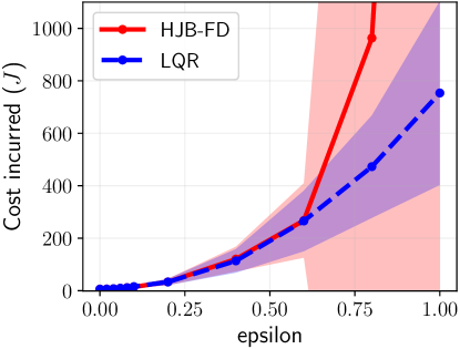
(a) Full noise spectrum.

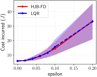
(b) Low noise region enhanced.

Figure 1: Performance comparison of the solution to HJB (Eq. (45)) obtained from finite difference scheme and LQR on the linear system. The mean and standard deviation of the cost incurred by the system are calculated from experiments for different cases of $\epsilon$. The data shown is from simulating the linear system from initial condition of $x(0)=1$.

In the following, we show the reason behind the inaccuracy of the HJB-FD solution. We first compare the expected cost-to-go values between the two methods for different cases of $\epsilon$. The expected cost-to-go for HJB is directly available from the solution to Eq. (45), over the entire domain. For LQR, we can calculate the expected cost-to-go for the stochastic case by solving the following standard equations (written specifically for our linear system in Eq. (46)):

$$J_{lqr}(t,x)=\frac{1}{2}p_{t}x^{2}+v_{t},$$ (47)

$$-\dot{p}_{t}=2p_{t}-\frac{p_{t}^{2}}{r}+q,~{}p_{T}=q_{T},$$ (48)

$$-\dot{v}_{t}=p_{t}(\epsilon\sigma)^{2},~{}v_{T}=0.$$ (49)

We show, in the left column of Fig. 2, the cost-to-go function of the HJB solution and the LQR solution in our domain at a specific time instant. We observe that the HJB-FD cost-to-go exactly matches the LQR for $\epsilon=0$ and $0.2$. For $\epsilon=1$, it can be seen that the cost-to-go values don’t match and we can infer that the HJB-FD solution is inaccurate. Since the feedback policy depends on the cost-to-go function, it will also be inaccurate in such cases.

The reason for the inaccuracy of the stochastic HJB-FD solution is illustrated in the right column of Fig. 2. The plots in the right column show the trajectories taken by the system under the HJB-FD feedback policy for different values of $\epsilon$. When the $\epsilon$ value parametrizing the strength of the noise becomes large, it can be seen that the trajectories leave the domain on which the solution is obtained, due to the noise acting on the system. Since the cost-to-go solution is unavailable outside the domain, one has to approximate the cost of these trajectories with the cost at the boundary. To get an accurate solution, the domain one has to solve needs to expand with time. Since most computational methods do a fixed domain approximation, the stochastic solution obtained will inherently be inaccurate because the states inside the boundary need the cost-to-go values of states outside the domain as the noise intensity increases. In the deterministic case, owing to the absence of noise, the control takes the system towards the origin and not outside the domain. So, the deterministic cost-to-go and feedback policy is always accurate. Furthermore, note that when the stochastic HJB solution is accurate, the system does not leave the domain owing to the control dominating the effect of the noise.

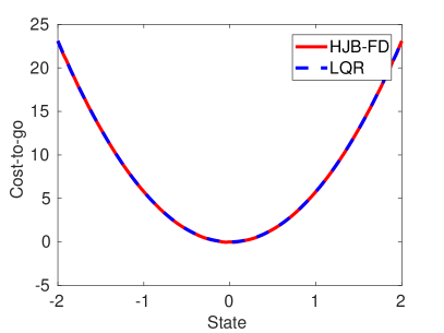
(a) $\epsilon=0$

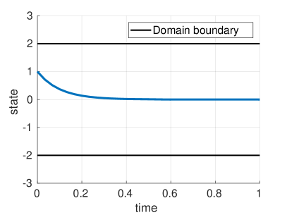
(b) $\epsilon=0$

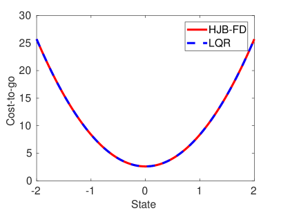
(c) $\epsilon=0.2$

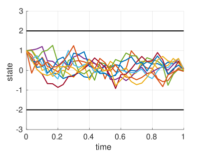
(d) $\epsilon=0.2$

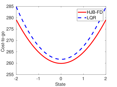
(e) $\epsilon=1$

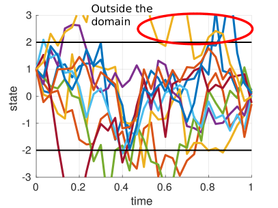
(f) $\epsilon=1$

Figure 2: Left column: Comparison of expected cost-to-go value from the HJB-FD solution and the LQR Riccati solution at $t=0.81$. The plot shows that the HJB-FD cost-to-go doesn’t match the LQR cost-to-go (which is the optimal) at high noise levels.
Right column: Sample trajectories of the linear system at different noise levels under the policy computed by HJB-FD. Since the trajectory could leave the domain in high noise cases, the expected cost-to-go calculated in seeking the stochastic feedback policy will be inaccurate. (The trajectories were generated with the original sampling time of the FD solver, but the data is plotted at a larger sampling interval for the sake of clarity.)

Nonlinear case

We consider the nonlinear system $dx=(-cos(x)+u)dt+\epsilon dw$ with initial condition $x(0)=1$. As discussed in section IV, MPC-SH feedback law is the optimal feedback law for the deterministic problem and the cost is $O(\epsilon^{4})$ near-optimal to the stochastic cost. It is also computationally feasible to solve the open-loop deterministic problem in practice, as opposed to solving the HJB, which is computationally intractable due to the curse of dimensionality. The algorithm for MPC-SH is given in Algorithm 1. To solve the open-loop optimization problem in MPC-SH, the iterative linear quadratic regulator (ILQR) algorithm is used [32]. ILQR is used specifically since the converged optimal solution satisfies the necessary conditions of the minimum principle given in eqs. (25), (26). As discussed in proposition 4, the deterministic open-loop problem has a unique minimum for our case, and ILQR will guarantee convergence to it [2].

We solve the HJB for the nonlinear system for a value of $\epsilon$ and test the obtained policy on the system for the same $\epsilon$ value on 100 experiments. The open-loop optimization in MPC-SH is solved using ILQR as discussed above for the specific initial condition and tested on the stochastic nonlinear system for a value of $\epsilon$. The experiment is repeated for different noise levels by varying $\epsilon$. The decision epoch time chosen for MPC-SH was $\Delta=0.005$, approximately $1000\times$ the $\Delta t$ used in FD. The mean and standard deviation of the cost incurred in these experiments are tabulated in Fig. 3. Fig. 3 shows that the MPC-SH feedback law has comparable performance with the stochastic HJB-FD solution. MPC-SH is also computationally more efficient to solve, as HJB-FD requires very fine time discretization to solve without numerical issues even for the 1-D case owing to the CFL conditions (see table I).

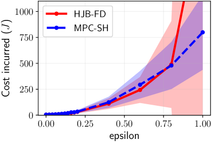
(a) Full noise spectrum.

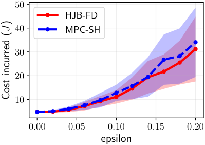
(b) Low noise region enhanced.

Figure 3: Performance comparison of HJB-FD and MPC-SH on the 1-D nonlinear system for different noise levels.

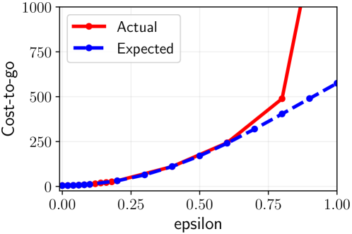
(a) HJB-FD cost-to-go.

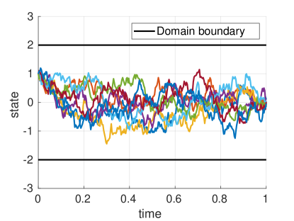
(b) $\epsilon=0.2$

(c) $\epsilon=0.8$

Figure 4: (a) Comparison of the expected cost-to-go obtained from the HJB-FD solution and the actual cost incurred by applying the HJB-FD feedback policy on the nonlinear system. The cost-to-go is obtained for the initial condition $x(0)=1$ and the actual cost is the average cost of 100 simulations. Trajectory samples of the nonlinear system under the HJB-FD policy for two different cases of $\epsilon$ are shown in (b) and (c).

Even when the deterministic solution, which MPC-SH is, is applied to the stochastic case, the performance is almost equivalent, due to the $O(\epsilon^{4})$ near-optimality of the deterministic solution to the stochastic. Moreover, the stochastic policy has higher variance than the deterministic MPC-SH policy at $\epsilon=0.8$, and fails after that - another case that shows that the calculated stochastic policy is inaccurate. To illustrate the inaccuracy in the HJB-FD solution, we compare the expected cost-to-go value calculated by solving the HJB with the true cost of operation in Fig. 4. It can be seen that the cost-to-go becomes inaccurate after $\epsilon=0.6$. As shown in Fig. 4c, the inaccuracy of the calculation is due to the unaccounted cost of the trajectories leaving the domain in high-noise cases.

V-B Comparison between MPC-SH and Optimal Linear feedback

In this section, we will show the comparison in performance of two different deterministic feedback laws: the optimal linear feedback and the MPC-SH feedback law. In remark 3, it was shown that the optimal linear feedback controller given by eqs. (33)-(35), designed around the optimal open-loop nominal trajectory is also near-optimal to the order of $O(\epsilon^{4})$ to the stochastic system. This design is referred to as the trajectory-optimized perturbation feedback controller (T-PFC) [23]. The difference between T-PFC and MPC-SH is that, T-PFC plans the nominal trajectory only once, from the initial state, and uses the linear feedback to correct for errors during its execution. While, MPC-SH replans the nominal trajectory from the current state continuously and uses the linear feedback only for a short interval $\Delta$ between the replans. The advantage of using T-PFC is that the open-loop optimization has to be carried out only once (preferably offline), and the precomputed linear feedback gains can be used to correct for deviations due to uncertainty online. In a stochastic setting, this optimal nominal trajectory generated initially is only optimal if the system stays close to the nominal. If it deviates, the trajectory has to be replanned from the current state as done by MPC-SH to maintain optimal performance. We will examine how the performance of T-PFC compares with MPC-SH in nonlinear robotics problems for different noise levels in Fig. 5.

In Fig. 5, we see that T-PFC shows comparable performance to MPC-SH for low values of $\epsilon$. As noise increases, the trajectory deviates from the nominal computed initially, and the feedback policy no longer is optimal, necessitating the need for a replanned nominal trajectory from the current state. Hence, the performance of T-PFC deteriorates for high noise levels. Nevertheless, there is value for T-PFC-like deterministic feedback laws in applications that wish to minimize onboard computing and act in low-noise settings.

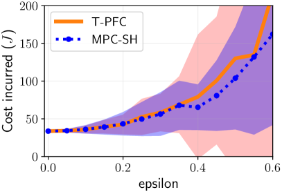
(a) Car-like robot

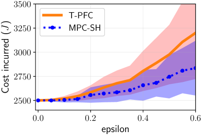
(b) Cartpole

Figure 5: Performance comparison of T-PFC with MPC-SH in nonlinear robotics systems. Both policies are computed for a specific initial condition and tested on 100 different samples for each value of $\epsilon$ to find the cost statistics.

V-C Discussion

The primary takeaway from Section V-A and V-B is that deterministic policies are not only near-optimal but also accurate, scalable, and repeatable. It is not possible to compute the stochastic policy accurately, as shown in Sec. V-A. Note that the inaccuracy is not a limitation of the finite difference method used. Galerkin Finite Element and Collocation methods like Chebyshev polynomial-based methods are also solved on a bounded domain, and consequently, not immune to the errors observed in FD. As discussed in Sec. IV, random sampling-based methods like approximate dynamic programming, and reinforcement learning are dependent on their samples to explore the domain and inherently have the same issue in the stochastic case. In high dimensions problems, one needs a prohibitively large number of samples to explore the domain. An inefficient sampling of the domain will lead to inaccurate policies as the cost-to-go is not accurately captured by the samples. Due to this issue, there is an inherent variance in the solution obtained by such methods [27]. We have done an exhaustive investigation comparing the deterministic feedback approach with other RL methods in the companion paper [2], where we report the accuracy, scalability, efficiency, and repeatability of the deterministic policy that the stochastic RL methods lack. To summarize, as shown in Fig. 2, the regime where the stochastic solutions can be computed accurately is the one of low noise where the deterministic solution gives near-identical performance, and consequently, in practice, the deterministic feedback is the best one can do.

VI Conclusion

In this paper, we have considered the problem of stochastic nonlinear control. We have shown that recursively solving the deterministic optimal control problem from the current state, à la MPC, results in a near-optimum policy to fourth order in a small noise parameter, and in practice, empirical evidence shows that the MPC law performs better than the law obtained by computationally solving the stochastic DP problem owing to the perturbation structure of the deterministic optimal control problem. An important limitation currently is the smoothness of the nominal trajectory such that suitable Taylor expansions are possible, this breaks down when trajectories are non-smooth such as in hybrid systems like legged robots, or maneuvers have kinks for car-like robots such as in a tight parking application. It remains to be seen as to if, and how, one may extend the result to such applications that are piecewise smooth in the dynamics. Also, a further careful investigation into the relative merits and demerits of the shrinking horizon approach to MPC when compared to the traditional fixed horizon approach is required, as is the generalization to the more practical and important partially observed problem.

VII Acknowledgement

This work was supported by the NSF under grants ECCS-1637889, CDSE 1802867, and the AFOSR DDIP program under grant FA9550-17-1-0068.

Author biography:

Mohamed Naveed Gul Mohamed is pursuing his Ph.D. in Aerospace Engineering at Texas A&M University, where he is also a member of the Estimation, Decision, and Planning Laboratory. He holds a bachelor’s degree in Instrumentation and Control Engineering from NIT Trichy, India.

Suman Chakravorty is a Professor of Aerospace Engineering at Texas A&M University. He holds a Ph.D. in Aerospace Engineering from the University of Michigan, Ann Arbor. His research interests broadly lie in Estimation and Stochastic Optimal Control Theory with application to Robotic Control and Situational Awareness Problems.

Raman Goyal earned his Ph.D. in Aerospace Engineering from Texas A&M University, College Station and his B.Tech. degree in Mechanical Engineering from IIT Roorkee, India. Raman is interested in intelligent learning approaches for optimal control of stochastic nonlinear systems. He has also worked on modeling, design, control, and security of various cyber-physical systems.

Ran Wang received his Ph.D. in Aerospace Engineering from Texas A&M University, College Station and his bachelor’s degree in Mechanical Engineering from Huazhong University of Science and Technology. Ran’s research interests include optimal control and reinforcement learning of soft-body robots.

Appendix A DETAILED PROOFS OF RESULTS

A-A Proof of Lemma 1

Proof:

We proceed by induction. The first general instance of the recursion occurs at $k=3$. It can be shown that:

$$\delta x_{3} =\underbrace{(\bar{A}_{2}\bar{A}_{1}(\epsilon\omega_{0}\sqrt{\Delta t})+\bar{A}_{2}(\epsilon\omega_{1}\sqrt{\Delta t})+\epsilon\omega_{2}\sqrt{\Delta t})}_{\delta x_{3}^{l}}+e_{3},$$

$$e_{3} =\bar{A}_{2}\bar{S}_{1}(\epsilon\omega_{0}\sqrt{\Delta t})+\bar{S}_{2}(\bar{A}_{1}(\epsilon\omega_{0}\sqrt{\Delta t})+\epsilon\omega_{1}\sqrt{\Delta t}+$$

$$\bar{S}_{1}(\epsilon\omega_{0}\sqrt{\Delta t})).$$

Noting that $\bar{S}_{1}(.)$ and $\bar{S}_{2}(.)$ are second and higher order terms, it follows that $e_{3}$ is $O(\epsilon^{2})$.
Suppose now that $\delta x_{k}=\delta x_{k}^{l}+e_{k}$ where $e_{k}$ is $O(\epsilon^{2})$. Then: $\delta x_{k+1}=\bar{A}_{k}(\delta x_{k}^{l}+e_{k})+\epsilon\omega_{k}\sqrt{\Delta t}+\bar{S}_{k}(\delta x_{k}),\\ =\underbrace{(\bar{A}_{k}\delta x_{k}^{l}+\epsilon\omega_{k}\sqrt{\Delta t})}_{\delta x_{k+1}^{l}}+\underbrace{\{\bar{A}_{k}e_{k}+\bar{S}_{k}(\delta x_{k})\}}_{e_{k+1}}.$ Noting that $\bar{S}_{k}$ is $O(\epsilon^{2})$ and that $e_{k}$ is $O(\epsilon^{2})$ by assumption, the result follows that $e_{k+1}$ is $O(\epsilon^{2})$.
Now, let us take a closer look at the term $e_{k}$ and again proceed by induction. It is clear that $e_{1}=e_{1}^{(2)}=0$. Next, it can be seen that $e_{2}=\bar{A}_{1}e_{1}^{(2)}+\delta x_{1}^{l^{\prime}}\bar{S}_{1}^{(2)}\delta x_{1}^{l}+O(\epsilon^{3})=(\epsilon^{2}\Delta t)\omega_{0}^{\prime}\bar{S}_{1}^{(2)}\omega_{0}+O(\epsilon^{3})$, which shows the recursion is valid for $k=2$ given it is so for $k=1$.
Suppose that it is true for $k$. Then: $\delta x_{k+1}=\bar{A}_{k}\delta x_{k}+\bar{S}_{k}(\delta x_{k})+\epsilon\omega_{k}\sqrt{\Delta t}=\bar{A}_{k}(\delta x_{k}^{l}+e_{k})+\bar{S}_{k}(\delta x_{k}^{l}+e_{k})+\epsilon\omega_{k}\sqrt{\Delta t}=\underbrace{(\bar{A}_{k}\delta x_{k}^{l}+\epsilon\omega_{k}\sqrt{\Delta t})}_{\delta x_{k+1}^{l}}+\underbrace{\bar{A}_{k}e_{k}^{(2)}+\delta x_{k}^{l^{\prime}}\bar{S}_{k}^{(2)}\delta x_{k}^{l}}_{e_{k+1}^{(2)}}+O(\epsilon^{3}),$where the last line follows because $e_{k}=e_{k}^{(2)}+O(\epsilon^{3})$, and $\bar{S}_{k}^{(2)}$ is the second order term of $\bar{S}_{k}(.)$. This completes the induction and the proof. ∎

A-B Proof of Lemma 2

Proof:

We have that: $\mathcal{J}^{\pi}=\sum_{k}\bar{c}_{k}+\sum_{k}\bar{C}_{k}(\delta x_{k}^{l}+e_{k})+\sum_{k}\bar{H}_{k}(\delta x_{k}^{l}+e_{k}),=\sum_{k}\bar{c}_{k}+\sum_{k}\bar{C}_{k}\delta x_{k}^{l}+\sum_{k}\delta x_{k}^{l^{\prime}}\bar{H}_{k}^{(2)}\delta x_{k}^{l}+\bar{C}_{k}e_{k}^{(2)}+O(\epsilon^{3}),$where the last line of the equation above follows from an application of Lemma 1. ∎

A-C Proof of Proposition 1

In order to prove this result, we first need the following preparatory result. Consider the following deterministic continuous time system:

$$J^{\pi}(0,x_{0}) =\int_{0}^{T}\underbrace{c(x_{t},\pi_{t}(x_{t})}_{\bar{c}(x_{t})}dt+c_{T}(x_{T}),$$

$$\dot{x} =\underbrace{f(x)+g(x)\pi_{t}(x)}_{\bar{f}(x)}+\epsilon v,$$

where $v(t)$ is a given continuous time input. We re-write the above policy evaluation equation in state-space form as follows:

$$\dot{x}=\bar{f}(x)+\epsilon v,\;\dot{R}=\bar{c}(x),\;\dot{t}=1,$$

$$Z(t)=R(t)+c_{T}(x),$$

where the above equations can now be expressed in a time-invariant state space form as: $\dot{X}=F(X)+\epsilon Gv$, and $Z(t)=H(X(t))$, where $X=[x,R,t]^{\prime}$, $F=[\bar{f}(x),\bar{c}(x),1]^{\prime}$, $G=[I_{n},0,0]^{\prime}$ and $H(X)=R+c_{T}(x)$.
Given that the component functions $f(\cdot,\cdot),c(\cdot,\cdot),c_{T}(\cdot),\pi_{t}(\cdot)$ are five times continuously differentiable ($\mathcal{C}^{5}$) in their arguments, the output $Z(T)=J^{\pi}(0,x_{0})$ can be expressed in terms of the inputs $v(t)$ as the unique Volterra series (Theorem 2.5 in [35]) where we have suppressed the dependence on $\pi$ for notational convenience:

$$Z(T)=J^{(0)}(x_{0})+\epsilon\int_{0}^{T}J^{(1)}(T,s)v(s)ds$$

$$+\epsilon^{2}\int_{0}^{T}\int_{0}^{s_{1}}J^{(2)}(T,s_{1},s_{2})v(s_{1})v(s_{2})ds_{2}ds_{1}$$

$$+\epsilon^{3}\int_{0}^{T}\int_{0}^{s_{1}}\int_{0}^{s_{2}}J^{(3)}(T,s_{1},s_{2},s_{3})v(s_{3})v(s_{2})v(s_{1})ds_{3}ds_{2}ds_{1}$$

$$+\epsilon^{4}\int_{0}^{T}\int_{0}^{s_{1}}\int_{0}^{s_{2}}\int_{0}^{s_{3}}J^{(4)}(T,s_{1},s_{2},s_{3},s_{4})[v(s_{4})v(s_{3})$$

$$\quad\quad v(s_{2})v(s_{1})]ds_{3}ds_{2}ds_{1}+\mathcal{G},$$ (50)

where the Volterra kernels $J^{(k)}(.)$ and $\mathcal{G}$ are unique, and $\mathcal{G}$ is an $o(\epsilon^{4})$ function.

Proof:

We show the result for a scalar input, the generalization to a vector input is straightforward. We first write the sample path cost in an input-output fashion in the discrete time case. Let $v(t)$ be a given input sequence, and given a discretization time $\Delta t$ such that $T=N\Delta t$, let $v_{k}=v(k\Delta t)$, $k=0,1,2\cdots N-1,$ denote a piecewise constant approximation of the input. Given sufficient smoothness ($\mathcal{C}^{5}$) of the requisite functions, the cost of any sample path from a given initial state $x_{0}$ can be expanded as follows in discrete time (where we have suppressed the explicit dependence of the different terms on $x_{0}$ for simplifying notation): $\mathcal{V}^{\pi}_{N}=\mathcal{V}^{\pi,0}_{N}+\epsilon\mathcal{V}^{\pi,1}_{N}+\epsilon^{2}\mathcal{V}^{\pi,2}_{N}+\epsilon^{3}\mathcal{V}^{\pi,3}_{N}+\epsilon^{4}\mathcal{V}^{\pi,4}_{N}+\mathcal{G}_{N}^{\pi},$where $\mathcal{V}^{\pi,0}_{N}$ represents the nominal/ zero input cost and

$$\mathcal{V}^{\pi,1}_{N}=\sum_{s=0}^{N-1}\mathcal{J}^{(1)}_{N}(N\Delta t,s\Delta t)v_{s}{\Delta t},$$

$$\mathcal{V}^{\pi,2}_{N}=\sum_{s_{1}=0}^{N-1}\sum_{s_{2}=0}^{s_{1}}\mathcal{J}^{(2)}_{N}(N\Delta t,s_{1}\Delta t,s_{2}\Delta t)v_{s_{2}}v_{s_{1}}\Delta t^{2},$$

$$\mathcal{V}^{\pi,3}_{N}=\sum_{s_{1}=0}^{N-1}\sum_{s_{2}=0}^{s_{1}}\sum_{s_{3}=0}^{s_{2}}\mathcal{J}^{(3)}_{N}(N\Delta t,s_{1}\Delta t,s_{2}\Delta t,s_{3}\Delta t)$$

$$\quad\quad\times v_{s_{3}}v_{s_{2}}v_{s_{1}}\Delta t^{3},$$

$$\mathcal{V}^{\pi,4}_{N}=\sum_{s_{1}=0}^{N-1}\sum_{s_{2}=0}^{s_{1}}\sum_{s_{3}=0}^{s_{2}}\sum_{s_{4}=0}^{s_{3}}\mathcal{J}^{(4)}_{N}(N\Delta t,s_{1}\Delta t,s_{2}\Delta t,s_{3}\Delta t,s_{4}\Delta t)$$

$$\quad\quad\times v_{s_{4}}v_{s_{3}}v_{s_{2}}v_{s_{1}}\Delta t^{4},$$

where $\mathcal{J}^{(k)}(.)$ represent the piecewise constant discretized kernels corresponding to the Volterra kernels defined in (50). Further, the remainder function $\mathcal{G}_{N}^{\pi}$ is an $o(\epsilon^{4})$ function.
Let $V^{\pi}(x_{0})$ denote the cost of the trajectory under the continuous time input $v(t)$. Then it follows that $\mathcal{V}^{\pi}_{N}(x_{0})\rightarrow V^{\pi}(x_{0})$ as $N\rightarrow\infty$, regardless of the input sequence $v(t)$. Therefore, it follows that the discretized piecewise constant kernels $\mathcal{J}^{(k)}_{N}\rightarrow J^{(k)}$ in the $L_{1}$ sense as $N\rightarrow\infty$.
If the inputs were a discretized Wiener sequence $w(k\Delta t)=\omega_{k}\sqrt{\Delta t}$, where $\omega_{k}$ is a Gaussian white noise sequence, we can write the cost of a sample path as: $\mathcal{J}^{\pi}_{N}=\mathcal{J}^{\pi,0}_{N}+\epsilon\mathcal{J}^{\pi,1}_{N}+\epsilon^{2}\mathcal{J}^{\pi,2}_{N}+\epsilon^{3}\mathcal{J}^{\pi,3}_{N}+\epsilon^{4}\mathcal{J}^{\pi,4}_{N}+\mathcal{R}_{N}^{\pi}$, where $\mathcal{J}^{\pi,0}_{N}$ is the zero noise cost and

$$\mathcal{J}^{\pi,1}_{N}=\sum_{s=0}^{N-1}\mathcal{J}^{(1)}_{N}(N\Delta t,s\Delta t)\omega_{s}{\sqrt{\Delta t}},$$

$$\mathcal{J}^{\pi,2}_{N}=\sum_{s_{1}=0}^{N-1}\sum_{s_{2}=0}^{s_{1}}\mathcal{J}^{(2)}_{N}(N\Delta t,s_{1}\Delta t,s_{2}\Delta t)\omega_{s_{2}}\omega_{s_{1}}\Delta t,$$

$$\mathcal{J}^{\pi,3}_{N}=\sum_{s_{1}=0}^{N-1}\sum_{s_{2}=0}^{s_{1}}\sum_{s_{3}=0}^{s_{2}}\Big{(}\mathcal{J}^{(3)}_{N}(N\Delta t,s_{1}\Delta t,s_{2}\Delta t,s_{3}\Delta t)$$

$$\quad\quad\omega_{s_{3}}\omega_{s_{2}}\omega_{s_{1}}(\Delta t)^{3/2}\Big{)},$$

$$\mathcal{J}^{\pi,4}_{N}=\sum_{s_{1}=0}^{N-1}\sum_{s_{2}=0}^{s_{1}}\sum_{s_{3}=0}^{s_{2}}\sum_{s_{4}=0}^{s_{3}}\Big{(}\mathcal{J}^{(4)}_{N}(N\Delta t,s_{1}\Delta t,s_{2}\Delta t,s_{3}\Delta t,$$

$$\quad\quad s_{4}\Delta t)\omega_{s_{4}}\omega_{s_{3}}\omega_{s_{2}}\omega_{s_{1}}(\Delta t)^{2}\Big{)},$$

Moreover, due to the whiteness of the noise sequence $\{\omega_{k}\}$, it follows that $E[\mathcal{J}^{\pi,1}_{N}]=0$, and $E[\mathcal{J}^{\pi,3}_{N}]=0$, since these terms are made of odd valued products of the noise sequences, while $E[\mathcal{J}^{\pi,2}_{N}],E[\mathcal{J}^{\pi,4}_{N}]$ are both finite owing to the finiteness of the moments of the noise values. Next as we take the limit of the terms above as $N\rightarrow\infty$, we obtain:

$$\lim_{N\rightarrow\infty}E[\mathcal{J}^{\pi,2}_{N}]=\int_{0}^{T}J^{(2)}(T,t,t)dt\equiv J^{\pi,1}<\infty,$$

$$\lim_{N\rightarrow\infty}E[\mathcal{J}^{\pi,4}_{N}]=\int_{0}^{T}\int_{0}^{t}J^{(4)}(T,t,t,\tau,\tau)d\tau dt\equiv J^{\pi,2}<\infty,$$

where the first equality above follows from the convergence of the discretized kernels $\mathcal{J}^{(k)}_{N}\rightarrow J^{(k)}$ for $k=2,4$, while the integrals are finite owing to the continuity of the functions $J^{(2)}$ and $J^{(4)}$ as established in (50). Further $\lim_{\epsilon\rightarrow 0}\epsilon^{-4}\lim_{N\rightarrow\infty}E[\mathcal{R}_{N}^{\pi}]=\lim_{N\rightarrow\infty}E[\lim_{\epsilon\rightarrow 0}\epsilon^{-4}\mathcal{R}_{N}^{\pi}]=0$, i.e., $\lim_{N\rightarrow\infty}E[\mathcal{R}_{N}^{\pi}]$ is $o(\epsilon^{4})$. Therefore, taking expectations on both sides, we obtain: $\lim_{N\rightarrow\infty}E[\mathcal{J}^{\pi}_{N}]={J}^{\pi,0}+\epsilon^{2}{J}^{\pi,1}+\epsilon^{4}{J}^{\pi,2}+o(\epsilon^{4}),$where $J^{\pi,0}=\lim_{N\rightarrow\infty}\mathcal{J}^{\pi,0}_{N}$, which proves the first part of the result.
Next, from Lemma 2, as we take the limit $\Delta t\rightarrow 0$, it is clear that ${J}^{\pi,0}$ stems solely from the continuous time nominal trajectory, and that ${J}^{\pi,1}$ is solely dependent on the continuous time linear closed loop state. Therefore, the result follows. ∎

A-D Proof of Proposition 2

Proof:

We first discretize the time by $\Delta t$ and obtain the final differential equations by taking the limit as $\Delta t\rightarrow 0$. Let $J_{k}(x)=J(k\Delta t,x)$ be a discretization of the cost function. Using Proposition 1, we know that any cost function, and hence, the optimal cost-to-go function can be expanded as:

$$J_{k}=J_{k}^{0}+\epsilon^{2}J_{k}^{1}+\epsilon^{4}J_{k}^{2}+\cdots.$$ (51)

Taking the dynamic system for the vector case which is given by

$$x_{k+1}=x_{k}+(\mathcal{F}(x)+\mathcal{G}(x)u)\Delta t+\epsilon\omega_{k}\sqrt{\Delta t},$$

and substituting the minimizing control $u=-{R}^{\mathsf{-1}}{\mathcal{G}(x)}^{\mathsf{T}}J^{x}_{k+1}$ into the dynamic programming Eq. (3) implies:

$$J_{k}(x)=\bar{l}\Delta t+\frac{1}{2}{(J^{x}_{k+1})}^{\mathsf{T}}\bar{\mathcal{G}}{R}^{\mathsf{-1}}{\bar{\mathcal{G}}}^{\mathsf{T}}(J^{x}_{k+1})\Delta t+{(J^{x}_{k+1})}^{\mathsf{T}}\bar{\mathcal{F}}\Delta t$$

$$-{(J^{x}_{k+1})}^{\mathsf{T}}\bar{\mathcal{G}}{R}^{\mathsf{-1}}{\bar{\mathcal{G}}}^{\mathsf{T}}(J^{x}_{k+1})\Delta t+\frac{\epsilon^{2}}{2}tr(J_{k+1}^{xx})\Delta t+J_{k+1}(x),$$ (52)

where $J_{k}^{x}$, and $J_{k}^{xx}$ denote the first and second derivatives of the cost-to go function. Also, $\bar{l}=l(x)$, $\bar{\mathcal{F}}=\mathcal{F}(x)$, $\bar{\mathcal{G}}=\mathcal{G}(x)$ and $tr()$ is the trace operator. Substituting Eq. (51) into Eq. (52) we obtain that:

$$(J_{k}^{0}+\epsilon^{2}J_{k}^{1}+\epsilon^{4}J_{k}^{2}+\cdots)=\bar{l}\Delta t+$$

$$\frac{1}{2}{(J^{0,x}_{k+1}+\epsilon^{2}J^{1,x}_{k+1}+\cdots)}^{\mathsf{T}}\bar{\mathcal{G}}{R}^{\mathsf{-1}}{\bar{\mathcal{G}}}^{\mathsf{T}}(J^{0,x}_{k+1}+\epsilon^{2}J^{1,x}_{k+1}+\cdots)\Delta t$$

$$+{(J_{k+1}^{0,x}+\epsilon^{2}J_{k+1}^{1,x}+\cdots)}^{\mathsf{T}}\bar{\mathcal{F}}\Delta t-\Big{(}{(J^{0,x}_{k+1}+\epsilon^{2}J^{1,x}_{k+1}+\cdots)}^{\mathsf{T}}$$

$$\bar{\mathcal{G}}{R}^{\mathsf{-1}}{\bar{\mathcal{G}}}^{\mathsf{T}}(J^{0,x}_{k+1}+\epsilon^{2}J^{1,x}_{k+1}+\cdots)\Delta t\Big{)}+\frac{\epsilon^{2}}{2}tr(J_{k+1}^{0,xx}$$

$$+\epsilon^{2}J_{k+1}^{1,xx}+\cdots)\Delta t+(J^{0}_{k+1}(x)+\epsilon^{2}J^{1}_{k+1}(x)+\cdots).$$ (53)

Now, we equate the $\epsilon^{0}$, $\epsilon^{2}$ terms on both sides to obtain perturbation equations for the cost functions $J_{k}^{0},J_{k}^{1},J_{k}^{2}\cdots$.
First, let us consider the $\epsilon^{0}$ term. Utilizing Eq. (53) above, we obtain:

$$J_{k}^{0} =\bar{l}\Delta t+\frac{1}{2}{(J^{0,x}_{k+1})}^{\mathsf{T}}\bar{\mathcal{G}}{R}^{\mathsf{-1}}{\bar{\mathcal{G}}}^{\mathsf{T}}(J^{0,x}_{k+1})\Delta t$$

$$+{(J^{0,x}_{k+1})}^{\mathsf{T}}\underbrace{(\bar{\mathcal{F}}-\bar{\mathcal{G}}{R}^{\mathsf{-1}}{\bar{\mathcal{G}}}^{\mathsf{T}}J^{0,x}_{k+1})}_{\bar{f}^{0}}\Delta t+J_{k+1}^{0},$$ (54)

with the terminal condition $J_{N}^{0}=c_{T}$, and where we have dropped the explicit reference to the argument of the functions $x$ for convenience. Rearranging terms, dividing by $\Delta t$ and taking the limit as $\Delta t\rightarrow 0$ gives:

$$\frac{\partial J^{0}}{\partial t} =\bar{l}+\frac{1}{2}{(J^{0,x})}^{\mathsf{T}}\bar{\mathcal{G}}{R}^{\mathsf{-1}}{\bar{\mathcal{G}}}^{\mathsf{T}}(J^{0,x})$$

$$+{(J^{0,x})}^{\mathsf{T}}\underbrace{(\bar{\mathcal{F}}-\bar{\mathcal{G}}{R}^{\mathsf{-1}}{\bar{\mathcal{G}}}^{\mathsf{T}}J^{0,x})}_{\bar{f}^{0}},$$ (55)

with terminal condition $J^{0}(T,x)=c_{T}(x)$.
Similarly, one can obtain the $J^{1}$ equations by equating the $O(\epsilon^{2})$ terms in Eq. (53) that:

$$\frac{\partial J^{1}}{\partial t}=\frac{1}{2}\Big{(}{(J^{1,x})}^{\mathsf{T}}\bar{\mathcal{G}}{R}^{\mathsf{-1}}{\bar{\mathcal{G}}}^{\mathsf{T}}(J^{0,x})\\ +{(J^{0,x})}^{\mathsf{T}}\bar{\mathcal{G}}{R}^{\mathsf{-1}}{\bar{\mathcal{G}}}^{\mathsf{T}}(J^{1,x})\Big{)}+{(J^{1,x})}^{\mathsf{T}}\bar{\mathcal{F}}-{(J^{1,x})}^{\mathsf{T}}\bar{\mathcal{G}}{R}^{\mathsf{-1}}{\bar{\mathcal{G}}}^{\mathsf{T}}J^{0,x}-\\ {(J^{0,x})}^{\mathsf{T}}\bar{\mathcal{G}}{R}^{\mathsf{-1}}{\bar{\mathcal{G}}}^{\mathsf{T}}J^{1,x}\Delta t+\frac{1}{2}tr(J^{0,xx}),$$ (56)

which after regrouping and cancelling some of the terms yields:

$$\frac{\partial J^{1}}{\partial t}={(J^{1,x})}^{\mathsf{T}}\underbrace{(\bar{\mathcal{F}}-\bar{\mathcal{G}}{R}^{\mathsf{-1}}{\bar{\mathcal{G}}}^{\mathsf{T}}J^{0,x})}_{=\bar{f}^{0}}+\frac{1}{2}tr(J^{0,xx}),$$ (57)

with terminal boundary condition $J^{1}(T,x)=0$. Note the perturbation structure of Eqs. (A-D) and (57), $J_{t}^{0}$ can be solved without knowledge of $J_{t}^{1},J_{t}^{2}$ etc, while $J_{t}^{1}$ requires knowledge only of $J_{t}^{0}$, and so on. In other words, the equations can be solved sequentially rather than simultaneously.

Now, let us consider the discretized deterministic policy $u_{k}^{d}(.)$ that is a result of solving the deterministic DP equation:

$$\phi_{k}(x)=\min_{u}[c(x,u)+\phi_{k+1}(x^{\prime})],$$ (58)

where $x^{\prime}=x+\bar{\mathcal{F}}\Delta t+\bar{\mathcal{G}}u\Delta t$, i.e., the deterministic system obtained by setting $\epsilon=0$ in Eq. (1), and $\phi_{t}$ represents the optimal cost-to-go of the deterministic system. Analogous to the stochastic case, $u_{k}^{d}=-{R}^{\mathsf{-1}}{\bar{\mathcal{G}}}^{\mathsf{T}}\phi_{k+1}^{x}$. Next, let $\varphi_{k}$ denote the cost-to-go of the deterministic policy $u_{k}^{d}(.)$ when applied to the stochastic system, i.e., Eq. (1) with $\epsilon>0$. Then, the cost-to-go of the deterministic policy, when applied to the stochastic system, satisfies:

$$\varphi_{k}=c(x,u_{k}^{d}(x))+E[\varphi_{k+1}(x^{\prime})],$$ (59)

where $x^{\prime}=\bar{\mathcal{F}}\Delta t+\bar{\mathcal{G}}u_{t}^{d}\Delta t+\epsilon\omega_{t}\sqrt{\Delta t}$. Substituting $u_{k}^{d}=-{R}^{\mathsf{-1}}{\bar{\mathcal{G}}}^{\mathsf{T}}\phi_{k+1}^{x}$ into the equation above implies that:

$$\varphi_{k} =\varphi_{k}^{0}+\epsilon^{2}\varphi_{k}^{1}+\epsilon^{4}\varphi_{k}^{2}+\cdots$$

$$=\bar{l}\Delta t+\frac{1}{2}{(\phi^{x}_{k+1})}^{\mathsf{T}}\bar{\mathcal{G}}{R}^{\mathsf{-1}}{\bar{\mathcal{G}}}^{\mathsf{T}}\phi^{x}_{k+1}\Delta t$$

$$+{(\varphi_{k+1}^{0,x}+\epsilon^{2}\varphi_{k+1}^{1,x}+\cdots)}^{\mathsf{T}}\bar{\mathcal{F}}\Delta t$$

$$-{(\varphi_{k+1}^{0,x}+\epsilon^{2}\varphi_{k+1}^{1,x}+\cdots)}^{\mathsf{T}}\bar{\mathcal{G}}{R}^{\mathsf{-1}}{\bar{\mathcal{G}}}^{\mathsf{T}}\phi_{k+1}^{x}\Delta t$$

$$+\frac{\epsilon^{2}}{2}tr(\varphi_{k+1}^{0,xx}+\epsilon^{2}\varphi_{k+1}^{1,xx}+\cdots)\Delta t$$

$$+(\varphi_{k+1}^{0}+\epsilon^{2}\varphi_{k+1}^{1}+\cdots).$$ (60)

As before, if we gather the terms for $\epsilon^{0}$, $\epsilon^{2}$ etc. on both sides of the above equation, we shall get the equations governing $\varphi_{k}^{0},\varphi_{k}^{1}$ etc. First, looking at the $\epsilon^{0}$ term in Eq. (60), dividing by $\Delta t$ and taking the limit as $\Delta t\rightarrow 0$, we obtain:

$$\frac{\partial\varphi^{0}}{\partial t}=\bar{l}+\frac{1}{2}{(\phi^{x})}^{\mathsf{T}}\bar{\mathcal{G}}{R}^{\mathsf{-1}}{\bar{\mathcal{G}}}^{\mathsf{T}}\phi^{x}+{(\varphi^{0,x})}^{\mathsf{T}}(\bar{\mathcal{F}}-\bar{\mathcal{G}}{R}^{\mathsf{-1}}{\bar{\mathcal{G}}}^{\mathsf{T}}\phi^{x}),$$ (61)

with the terminal condition $\varphi(T,x)=c_{T}(x)$. However, the deterministic cost-to-go function also satisfies:

$$\frac{\partial\phi}{\partial t}=\bar{l}+\frac{1}{2}{(\phi^{x})}^{\mathsf{T}}\bar{\mathcal{G}}{R}^{\mathsf{-1}}{\bar{\mathcal{G}}}^{\mathsf{T}}\phi^{x}+{(\phi^{x})}^{\mathsf{T}}(\bar{\mathcal{F}}-\bar{\mathcal{G}}{R}^{\mathsf{-1}}{\bar{\mathcal{G}}}^{\mathsf{T}}\phi^{x}),$$ (62)

with terminal boundary condition $\phi(T,x)=c_{T}(x)$. Comparing Eqs. (61) and (62), it follows that $\phi(t,x)=\varphi^{0}(t,x)$ for all $t$. Further, comparing them to Eq. (A-D), it follows that $\varphi^{0}(t,x)=J^{0}(t,x)$, for all $(t,x)$. Also, note that the closed-loop system above, $\bar{\mathcal{F}}-\bar{\mathcal{G}}{R}^{\mathsf{-1}}{\bar{\mathcal{G}}}^{\mathsf{T}}\phi_{k+1}^{x}=\bar{f}^{0}$ (see Eq. (A-D) and (57)).

Next let us consider the $\epsilon^{2}$ terms in Eq. (60). We obtain: $\varphi_{k}^{1}={(\varphi_{k+1}^{1,x})}^{\mathsf{T}}(\bar{\mathcal{F}}-\bar{\mathcal{G}}{R}^{\mathsf{-1}}{\bar{\mathcal{G}}}^{\mathsf{T}}\phi_{k+1}^{x})\Delta t+\frac{1}{2}tr(\varphi_{k+1}^{0,xx})+\varphi_{k+1}^{1}.$ Noting that $\phi_{k}=\varphi_{k}^{0}$, implies that (after collecting terms and taking the limit as $\Delta t\rightarrow 0$):

$$\frac{\partial\varphi^{1}}{\partial t}={(\varphi^{1,x})}^{\mathsf{T}}\bar{f}^{0}+\frac{1}{2}tr(\varphi^{0,xx}),$$ (63)

with terminal condition $\varphi^{1}(T,x)=0$. Again, comparing Eq. (63) to Eq. (57), and noting that $\varphi^{0}=J^{0}$, it follows that $\varphi^{1}(t,x)=J^{1}(t,x)$, for all $(t,x)$. This completes the proof of the result.
∎

The result above has used the fact that the noise sequence $\omega_{t}$ is white. However, this is not necessary to show that $J_{t}^{0}(x)=\varphi_{t}^{0}(x)$ for all $(t,x)$.

A-E Proof of Proposition 3

Proof:

For simplicity, we first develop the result for the general scalar case and then show the derivation for the vector case. Let us start by writing the expansion around the nominal using the first Lagrange-Charpit equation (25) as:

$$\underbrace{\frac{d}{dt}(\bar{x}_{t}+\delta x_{t})}_{\dot{\bar{x}}_{t}+\dot{\delta x}_{t}}=\underbrace{f(\bar{x}_{t}+\delta x_{t})}_{(\bar{f}_{t}+\bar{f}_{t}^{x}\delta x_{t}+O(\delta x^{2}))}$$

$$-\frac{1}{r}(\bar{g}_{t}+\bar{g}_{t}^{x}\delta x_{t}+O(\delta x^{2}))^{2}(G_{t}+P_{t}\delta x_{t}+O(\delta x^{2})),$$ (64)

where $\bar{f}_{t}=f(\bar{x}_{t}),\bar{f}_{t}^{x}=\frac{\partial f}{\partial x_{t}}|_{\bar{x}_{t}},\bar{g}_{t}^{x}=\frac{\partial g}{\partial x_{t}}|_{\bar{x}_{t}}$. Expanding in powers of the perturbation variable $\delta x_{t}$, the equation above can be written as (after noting that $\dot{\bar{x}}_{t}=\bar{f}_{t}-\frac{\bar{g}_{t}^{2}}{r}G_{t}$ due to the nominal trajectory $\bar{x}_{t}$ satisfying the characteristic equation):

$$\dot{\delta x}_{t}=\left(\bar{f}_{t}^{x}-\frac{2\bar{g}_{t}\bar{g}_{t}^{x}}{r}G_{t}-\frac{\bar{g}_{t}^{2}}{r}P_{t}\right)\delta x_{t}+O(\delta x_{t}^{2}).$$ (65)

Next, we have: $\frac{dq}{dt}=-l^{x}+\frac{gg^{x}}{r}q^{2}-f^{x}q,$

$$\frac{d}{dt}(G_{t}+P_{t}\delta x_{t}+O(\delta x^{2}))=-(\bar{l}_{t}^{x}+\bar{l}_{t}^{xx}\delta x_{t}+O(\delta x^{2}))+$$

$$\frac{1}{r}(\bar{g}_{t}+\bar{g}_{t}^{x}\delta x_{t}+O(\delta x^{2}))(\bar{g}^{x}_{t}+\bar{g}_{t}^{xx}\delta x_{t}+O(\delta x^{2}))(G_{t}+P_{t}\delta x_{t}$$

$$+O(\delta x^{2}))^{2}-(\bar{f}_{t}^{x}+\bar{f}_{t}^{xx}\delta x_{t}+O(\delta x^{2}))(G_{t}+P_{t}\delta x_{t}+O(\delta x^{2})),$$ (66)

where $\bar{f}_{t}^{xx}=\frac{\partial^{2}f}{\partial x^{2}}|_{\bar{x}_{t}},\bar{g}_{t}^{xx}=\frac{\partial^{2}g}{\partial x^{2}}|_{\bar{x}_{t}},\bar{l}^{x}_{t}=\frac{\partial l}{\partial x}|_{\bar{x}_{t}},\bar{l}^{xx}_{t}=\frac{\partial^{2}l}{\partial x^{2}}|_{\bar{x}_{t}}$. Using $\frac{d}{dt}P_{t}\delta x_{t}=\dot{P}_{t}\delta x_{t}+P_{t}\dot{\delta x}_{t}$, substituting for $\dot{\delta x}_{t}$ from (27), and expanding the two sides above in powers of $\delta x_{t}$ yields:

$$\dot{G}_{t}+\left(\dot{P}_{t}+P_{t}(\bar{f}_{t}^{x}-\frac{2\bar{g}_{t}\bar{g}_{t}^{x}}{r}G_{t}-\frac{\bar{g}_{t}^{2}}{r}P_{t})\right)\delta x_{t}+O(\delta x^{2})\\ =-(\bar{l}_{t}^{x}-\frac{1}{r}\bar{g}_{t}\bar{g}_{t}^{x}G_{t}^{2}+\bar{f}_{t}^{x}G_{t})-(\bar{l}_{t}^{xx}-\frac{1}{r}\bar{g}_{t}\bar{g}_{t}^{xx}G_{t}^{2}-\frac{1}{r}\bar{g}_{t}^{x}\bar{g}_{t}^{x}G_{t}^{2}-\\ \frac{2}{r}\bar{g}_{t}\bar{g}_{t}^{x}G_{t}P_{t}+\bar{f}_{t}^{x}P_{t}+\bar{f}_{t}^{xx}G_{t})\delta x_{t}+O(\delta x^{2}).$$ (67)

Equating the first two powers of $\delta x_{t}$ yields:

$$\dot{G}_{t}+\bar{l}_{t}^{x}-\frac{1}{r}\bar{g}_{t}\bar{g}_{t}^{x}G_{t}^{2}+\bar{f}_{t}^{x}G_{t}=0,$$ (68)

$$\dot{P}_{t}+P_{t}\bar{f}_{t}^{x}+\bar{f}_{t}^{x}P_{t}+l_{t}^{xx}+[\bar{f}_{t}^{xx}-\frac{1}{r}\bar{g}_{t}^{xx}\bar{g}_{t}G_{t}]G_{t}-\frac{2\bar{g}_{t}\bar{g}_{t}^{x}}{r}G_{t}P_{t}$$

$$-P_{t}\frac{\bar{g}_{t}^{2}}{r}P_{t}-\frac{1}{r}\bar{g}_{t}^{x}\bar{g}_{t}^{x}G_{t}^{2}-\frac{2}{r}\bar{g}_{t}\bar{g}_{t}^{x}G_{t}P_{t}=0.$$ (69)

We can see that the first equation for $G_{t}$ is simply a restatement of the co-state equations in the Minimum Principle. Now, the optimal feedback law is given by:

$$u_{t}(x_{t}) =-\frac{g}{r}J_{x}$$

$$=-\frac{1}{r}(\bar{g}_{t}+\bar{g}_{t}^{x}\delta x_{t}+\cdots)(G_{t}+P_{t}\delta x_{t}+\cdots),$$ (70)

$$=-\frac{\bar{g}_{t}}{r}G_{t}+(-\frac{\bar{g}_{t}}{r}P_{t}-\frac{\bar{g}_{t}^{x}}{r}G_{t})\delta x_{t}+O(\delta x_{t}^{2}),$$ (71)

$$=\bar{u}_{t}+K_{t}\delta x_{t}+O(\delta x_{t}^{2}),$$ (72)

with $\bar{u}_{t}=-\frac{\bar{g}_{t}}{r}G_{t}$, and $K_{t}=-\frac{\bar{g}_{t}}{r}P_{t}-\frac{\bar{g}_{t}^{x}}{r}G_{t}$. Using the definition of $\bar{u}_{t}$, equation (69) can again be written as:

$$\dot{P}_{t}+P_{t}(\bar{f}_{t}^{x}+\bar{g}_{t}^{x}\bar{u}_{t})+(\bar{f}_{t}^{x}+\bar{g}_{t}^{x}\bar{u}_{t})P_{t}+l_{t}^{xx}+$$

$$[\bar{f}_{t}^{xx}+\bar{g}_{t}^{xx}\bar{u}_{t}]G_{t}-P_{t}\frac{\bar{g}_{t}^{2}}{r}P_{t}-\frac{1}{r}\bar{g}_{t}^{x}\bar{g}_{t}^{x}G_{t}^{2}-\frac{2}{r}\bar{g}_{t}\bar{g}_{t}^{x}G_{t}P_{t}=0.$$ (73)

which can again be written using $K_{t}$ and the following definition of $A_{t}=\bar{f}_{t}^{x}+\bar{g}_{t}^{x}\bar{u}_{t}$ as:

$$\dot{P}_{t}+P_{t}A_{t}+A_{t}P_{t}+l_{t}^{xx}+[\bar{f}_{t}^{xx}+\bar{g}_{t}^{xx}\bar{u}_{t}]G_{t}-K_{t}rK_{t}=0.$$ (74)

This is similar to LQR Riccati equation, except for the second order term $[\bar{f}_{t}^{xx}+\bar{g}_{t}^{xx}\bar{u}_{t}]G_{t}$ and the change in the feedback gain $K_{t}=-\frac{\bar{g}_{t}}{r}P_{t}-\frac{\bar{g}_{t}^{x}}{r}G_{t}$. This clearly shows that the feedback design is not an LQR design.

Proof for Vector Case: Let the system model be given as $\dot{x}=\mathcal{F}(x)+\mathcal{G}(x)u$ where, the control influence matrix $\mathcal{G}=\begin{bmatrix}g_{1}^{1}(x)\cdots g_{1}^{p}(x)\\ \ddots\\ g_{n}^{1}(x)\cdots g_{n}^{p}(x)\end{bmatrix}=\begin{bmatrix}\Gamma^{1}(x)\cdots\Gamma^{p}(x)]\end{bmatrix}$, i.e., $\Gamma^{j}$ represents the control influence vector corresponding to the $j^{th}$ input. Let $\bar{\mathcal{G}}_{t}=\mathcal{G}(\bar{x}_{t})$, where $\{\bar{x}_{t}\}$ represents the optimal nominal trajectory. Further, let $\mathcal{F}=\begin{bmatrix}f_{1}(x)\\ \vdots\\ f_{n}(x)\end{bmatrix}$ denote the drift of the system. Let $G_{t}=[G_{t}^{1}\cdots G_{t}^{n}]^{\intercal}$, and $R^{-1}\bar{\mathcal{G}}_{t}^{\intercal}G_{t}=[\bar{u}_{t}^{1}\cdots\bar{u}_{t}^{p}]^{\intercal}$, denote the optimal nominal co-state and control vectors respectively. Let $\bar{\mathcal{F}}_{t}^{x}=\begin{bmatrix}\frac{\partial f_{1}}{\partial x_{1}}\cdots\frac{\partial f_{1}}{\partial x_{n}}\\ \ddots\\ \frac{\partial f_{n}}{\partial x_{1}}\cdots\frac{\partial f_{n}}{\partial x_{n}}\end{bmatrix}|_{\bar{x}_{t}}$, and similarly $\bar{\Gamma}^{j,x}_{t}=\nabla_{x}\Gamma^{j}|_{\bar{x}_{t}}$. Further, define: $\bar{\mathcal{F}}_{t}^{xx,i}=\begin{bmatrix}\frac{\partial^{2}f_{1}}{\partial x_{1}\partial x_{i}}\cdots\frac{\partial^{2}f_{1}}{\partial x_{n}\partial x_{i}}\\ \ddots\\ \frac{\partial^{2}f_{n}}{\partial x_{1}\partial x_{i}}\cdots\frac{\partial^{2}f_{n}}{\partial x_{n}\partial x_{i}}\end{bmatrix}|_{\bar{x}_{t}},$ and $\bar{\Gamma}^{j,xx,i}_{t}$ similarly for the vector function $\Gamma^{j}$, and $\bar{\mathcal{G}}_{t}^{x,i}=\begin{bmatrix}\frac{\partial g_{1}^{1}}{\partial x_{i}}\cdots\frac{\partial g_{1}^{p}}{\partial x_{i}}\\ \ddots\\ \frac{\partial g_{n}^{1}}{\partial x_{i}}\cdots\frac{\partial g_{n}^{p}}{\partial x_{i}}\end{bmatrix}|_{\bar{x}_{t}}$. Finally, define $\mathcal{A}_{t}=\bar{\mathcal{F}}_{t}^{x}+\sum_{j=1}^{p}\bar{\Gamma}_{t}^{j,x}\bar{u}_{t}^{j}$, $\bar{L}_{t}^{x}=\nabla_{x}l|_{\bar{x}_{t}}$, and $\bar{L}_{t}^{xx}=\nabla^{2}_{xx}l|_{\bar{x}_{t}}$.
Using indicial notation, the Lagrange-Charpit equations are (the subscript $t$ is ignored for the sake of simplicity):

$$\dot{x}_{i} =f_{i}(x)-\Gamma_{i}^{j}{R}^{\mathsf{-1}}_{jm}\Gamma_{m}^{n}q_{n},$$ (75)

$$\dot{q}_{i} =-L_{i}^{x}-f_{ij}^{x}q_{j}+q_{n}\Gamma_{m}^{n}{R}^{\mathsf{-1}}_{lm}\Gamma^{l,x}_{ik}q_{k}.$$ (76)

Performing a perturbation expansion of $\dot{x}$ around a nominal trajectory $\bar{x}$ gives

$$\delta\dot{x}_{i}=(f_{ij}^{x}-\Gamma_{ij}^{k,x}{R}^{\mathsf{-1}}_{km}\Gamma_{m}^{n}q_{n}-\Gamma_{k}^{i}{R}^{\mathsf{-1}}_{km}\Gamma_{nj}^{m,x}q_{n})\delta x_{j}\\ +\frac{1}{2}(f_{ijk}^{xx}-{R}^{\mathsf{-1}}_{lm}\Gamma_{m}^{n}q_{n}\Gamma_{ikj}^{l,xx}-\Gamma_{ik}^{l,x}{R}^{\mathsf{-1}}_{lm}\Gamma_{nj}^{m,x}q_{n}\\ -\Gamma_{i}^{l}{R}^{\mathsf{-1}}_{lm}\Gamma_{nkj}^{m,xx}q_{n})\delta x_{k}\delta x_{j}-\Gamma_{i}^{j}{R}^{\mathsf{-1}}_{jm}\Gamma_{m}^{n}\delta q_{n}+\tilde{H}(\delta x^{3})+\tilde{S}(\delta q^{2}).$$ (77)

Expanding the co-states about the nominal gives

$$q_{i} =G_{i}+P_{ij}\delta x_{j}+H(\delta x^{2}),$$ (78)

$$\delta q_{i} =P_{ij}\delta x_{j}+H(\delta x^{2}).$$ (79)

Substituting Eq. (78) and (79) in Eq. (77), we get

$$\delta\dot{x}_{i} =(\bar{f}_{ij}^{x}-\bar{\Gamma}_{ij}^{k,x}{R}^{\mathsf{-1}}_{km}\bar{\Gamma}_{m}^{n}q_{n}-\bar{\Gamma}_{k}^{i}{R}^{\mathsf{-1}}_{km}\bar{\Gamma}_{nj}^{m,x}q_{n}$$

$$-\bar{\Gamma}_{i}^{l}{R}^{\mathsf{-1}}_{lm}\bar{\Gamma}_{m}^{n}P_{nj})\delta x_{j}+H.O.T.$$ (80)

Let $\mathcal{M}_{ij}=\bar{f}_{ij}^{x}-\bar{\Gamma}_{ij}^{k,x}{R}^{\mathsf{-1}}_{km}\bar{\Gamma}_{m}^{n}q_{n}-\bar{\Gamma}_{k}^{i}{R}^{\mathsf{-1}}_{km}\bar{\Gamma}_{nj}^{m,x}q_{n}-\bar{\Gamma}_{i}^{l}{R}^{\mathsf{-1}}_{lm}\bar{\Gamma}_{m}^{n}P_{nj}.$ Differentiating Eq. (78) and using Eq. (80), we get

$$\dot{q}_{i} =\dot{G}_{i}+P_{ij}\delta\dot{x}_{j}+\dot{P}_{ij}\delta x_{j}+\cdots,$$ (81)

$$\dot{q}_{i} =\dot{G}_{i}+P_{ij}(\mathcal{M}_{jk}\delta x_{k}+\cdots)+\dot{P}_{ij}\delta x_{j}+\cdots.$$ (82)

Expanding Eq. (76) upto 1st order about a nominal trajectory and substituting Eq. (78),

$$\dot{q}_{i} =-(\bar{L}_{i}^{x}-L_{ij}^{xx}\delta{x}_{j}+\cdots)-\bar{f}_{ij}^{x}(G_{j}+P_{jk}\delta x_{k}+\cdots)$$

$$-\delta x_{m}\bar{f}_{ijm}^{xx}(G_{j}+P_{ij}\delta x_{k}+\cdots)+(G_{n}+P_{nk}\delta x_{k}+\cdots)$$

$$\times(\bar{\Gamma}_{m}^{n}{R}^{\mathsf{-1}}_{lm}\bar{\Gamma}_{ip}^{l,x}+\bar{\Gamma}_{mj}^{n,x}\delta x_{j}{R}^{\mathsf{-1}}_{lm}\bar{\Gamma}_{ip}^{l,x}+\bar{\Gamma}_{m}^{n}{R}^{\mathsf{-1}}_{lm}\bar{\Gamma}_{ipj}^{l,xx}\delta x_{j}+\cdots)$$

$$\times(G_{p}+P_{pr}\delta x_{r}+\cdots).$$ (83)

Comparing the terms up to 1st order in $\delta x$ in Eq. (82) and Eq. (83) with appropriate change in indices, we get

$$\dot{G}_{i}=-\bar{L}_{i}^{x}-\bar{f}_{ij}^{x}G_{j}+G_{n}\bar{\Gamma}_{m}^{n}{R}^{\mathsf{-1}}_{lm}\bar{\Gamma}_{ip}^{l,x}G_{p},$$ (84)

$$\dot{P}_{ij}=-P_{ik}(\bar{f}_{kj}^{x}-\bar{\Gamma}_{kj}^{l,x}{R}^{\mathsf{-1}}_{lm}\bar{\Gamma}_{m}^{n}G_{n})-(\bar{f}_{ik}^{x}-G_{n}\bar{\Gamma}_{m}^{n}{R}^{\mathsf{-1}}_{lm}\bar{\Gamma}_{ik}^{l,x})P_{kj}$$

$$-L_{ij}^{xx}-(\bar{f}_{ipj}^{xx}-G_{n}\bar{\Gamma}_{m}^{n}{R}^{\mathsf{-1}}_{lm}\bar{\Gamma}_{ipj}^{l,xx})G_{p}+P_{ik}\bar{\Gamma}_{l}^{k}{R}^{\mathsf{-1}}_{lm}\bar{\Gamma}_{nj}^{m,x}G_{n}$$

$$+P_{ik}\bar{\Gamma}_{k}^{l}{R}^{\mathsf{-1}}_{lm}\bar{\Gamma}_{m}^{n}P_{nj}+P_{nj}\bar{\Gamma}_{m}^{n}{R}^{\mathsf{-1}}_{lm}\bar{\Gamma}_{ip}^{l,x}G_{p}$$

$$+G_{n}\bar{\Gamma}_{mj}^{n,x}{R}^{\mathsf{-1}}_{lm}\bar{\Gamma}_{ip}^{l,x}G_{p}.$$ (85)

Substituting $\bar{u}_{l}=-{R}^{\mathsf{-1}}_{lm}\bar{\Gamma}_{m}^{n}G_{n}$ and changing indices to group terms, Eq. (84) can be written as $\dot{G}_{i}=-\bar{L}_{i}^{x}-(\bar{f}_{ij}^{x}+\bar{u}_{l}\bar{\Gamma}_{ij}^{l,x})G_{j},$ whose vector form is Eq. (33). Similarly, $\bar{u}_{l}$ can be substituted in Eq. (85) and can be written as

$$\dot{P}_{ij} =-P_{ik}(\bar{f}_{kj}^{x}+\bar{\Gamma}_{kj}^{l,x}\bar{u}_{l})-(\bar{f}_{ik}^{x}+\bar{u}_{l}\bar{\Gamma}_{ik}^{l,x})P_{kj}-L_{ij}^{xx}$$

$$-(\bar{f}_{ipj}^{xx}-\bar{u}_{l}\bar{\Gamma}_{ipj}^{l,xx})G_{p}+K_{li}R_{lm}K_{mj}$$ (86)

where,

$$K_{ij}=-{R}^{\mathsf{-1}}_{im}(\bar{\Gamma}_{k}^{m}P_{kj}+\bar{\Gamma}_{kj}^{m,x}G_{k}).$$ (87)

Eq. (34) and Eq. (35) are the vector form of Eq. (86) and Eq. (87) respectively.

∎

A-F Proof of Proposition 4

Proof:

We show the scalar case, the vector case is a straightforward extension. We need the function $F(t,x,p,q,J)=p+l-\frac{1}{2}\frac{g^{2}}{r}q^{2}+fq$ to be $\mathcal{C}^{2}$ in all its arguments for unique characteristic curves, i.e., characteristic curves that do not intersect, since then the functions $F_{x}$ and $F_{q}$ are $\mathcal{C}^{1}$, and therefore Lipschitz continuous. From the existence and uniqueness results of ODEs [36], it follows that the Lagrange-Charpit characteristic ODEs $\dot{x}=F_{q}$, $\dot{q}=-F_{x}-qF_{J}$, are Lipschitz continuous in their right hand side functions, and therefore, have unique solutions. Moreover, the state $x$ and co-state $q=J^{x}$ vary continuously with respect to the terminal condition $x_{T}$ at any time $t$. Let us denote $q_{T}=c_{T}^{x}(x_{T})\equiv\phi_{T}(x_{T})$. Thus, $q_{T}$ is a function of $x_{T}$, i.e., $q_{T}$ is uniquely determined by the value of $x_{T}$.
Next, we show that under the Lagrange-Charpit equations, the function $\phi_{T}(x_{T})$ remains a function, i.e., we can write $q_{t}=\phi_{t}(x_{t})$, for some suitable smooth function $\phi_{t}(.)$, for any $t\in[0,T]$. In order to show this, suppose that this is not the case for some $t$. Then, it is necessary that there exist $x_{t}^{*}$ such that $\frac{dq_{t}}{dx_{t}}|_{x_{t}^{*}}=\pm\infty$, or equivalently that $\frac{dx_{t}}{dq_{t}}|_{x_{t}^{*}}=0$ (see Fig. 6). This in turn implies that there exists a terminal condition $x_{T}^{*}$ such that $\frac{dx_{t}}{dx_{T}}|_{x_{T}^{*}}=0$, where the terminal state $x_{T}^{*}$ maps to the state $x_{t}^{*}$ under the Lagrange-Charpit equations. We will now show that this is not feasible. Owing to the uniqueness of the solutions of the Lagrange-charpit equations: the Jacobian $\begin{vmatrix}\frac{\partial x_{t}}{\partial x_{T}}&\frac{\partial x_{t}}{\partial q_{T}}\\ \frac{\partial q_{t}}{\partial x_{T}}&\frac{\partial q_{t}}{\partial q_{T}}\end{vmatrix}_{(x_{T},q_{T})}\neq 0$, for any $(x_{T},q_{T})$. Thus, for $q_{T}=\phi_{T}(x_{T})$, substituting into the above equation implies that:

$$\frac{\partial x_{t}}{\partial x_{T}}-\phi_{T}^{\prime}(x_{T})\frac{\partial x_{t}}{\partial q_{T}}\neq 0,$$ (88)

for any terminal state $x_{T}$, where $\phi_{T}^{\prime}(.)$ represents the derivative of the function. Consider now the state $x_{T}^{*}$, owing to the fact that $\frac{dx_{t}}{dx_{T}}|_{x_{T}^{*}}=0$, we obtain that:

$$\frac{dx_{t}}{dx_{T}}=\frac{\partial x_{t}}{\partial x_{T}}\frac{dx_{T}}{dx_{T}}+\frac{\partial x_{t}}{\partial q_{T}}\frac{dq_{T}}{dx_{T}}=\frac{\partial x_{t}}{\partial x_{T}}+\phi_{T}^{\prime}(x_{T}^{*})\frac{\partial x_{t}}{\partial q_{T}}=0,$$ (89)

where the partial derivatives are taken at $x_{T}^{*}$. The above implies that $\frac{dq_{T}}{dx_{T}}=-\phi_{T}^{\prime}(x_{T}^{*})$, however, by definition: $\frac{dq_{T}}{dx_{T}}=\phi_{T}^{\prime}(x_{T}^{*})$, which means that $\phi_{T}^{\prime}(x_{T}^{*})=0$. Owing to Eq. (88), this means that $\frac{\partial x_{t}}{\partial x_{T}}|_{x_{T}^{*}}\neq 0$. However, using the second equality in Eq. (89), this implies that $\frac{dx_{t}}{dx_{T}}|_{x_{T}^{*}}\neq 0$, which contradicts the assumption that $\frac{dx_{t}}{dx_{T}}|_{x_{T}^{*}}=0$. Thus, it follows that $q_{t}=\phi_{t}(x_{t})$, for some smooth function $q_{t}(.)$, for any $t\in[0,T]$.

Figure 6: Mapping of the terminal conditions under the Lagrange Charpit equations. For two characteristic curves to flow through the same state $\bar{x}_{t}$, the $\phi_{t}(.)$ curve has to fold on itself necessitating the existence of a state $x_{t}^{*}$ such that $\frac{dx_{t}}{dq_{t}}|_{x_{t}^{*}}=0$. Given that the Lagrange-Charpit equations have unique solutions, such a state $x_{t}^{*}$ cannot exist.

Next, note that if a characteristic curve flows through the initial state $x_{0}$, then it means that we have found a terminal state $x_{T}$, along with the terminal co-state $q_{T}=c_{T}^{x}(x_{T})$, that satisfies the Lagrange-Charpit equations. However, this is, by definition, a solution that is found by satisfying the Minimum Principle. Therefore, owing to the development above, the co-state $q_{0}=\phi_{0}(x_{0})$ is uniquely determined by the initial state $x_{0}$, and a solution that satisfies the minimum principle is necessarily unique. Moreover, since this solution is the unique characteristic curve of the HJB flowing through $x_{0}$, it is also the global optimum.
The arguments made above can be generalized to the vector case where the function $F(t,x,J,p,q)$ in the vector case is defined as $F(t,x,J,p,q)=p+l-\frac{1}{2}{q}^{\mathsf{T}}\mathcal{G}(x){R}^{\mathsf{-1}}{\mathcal{G}(x)}^{\mathsf{T}}q+{q}^{\mathsf{T}}\mathcal{F}(x),$ and the equivalent Lagrange-Charpit characteristic ODEs are: $\dot{x}_{i}=f_{i}(x)-\Gamma_{i}^{j}{R}^{\mathsf{-1}}_{jm}\Gamma_{m}^{n}q_{n},\ \dot{q}_{i}=-L_{i}^{x}-f_{ij}^{x}q_{j}+q_{n}\Gamma_{m}^{n}{R}^{\mathsf{-1}}_{lm}\Gamma^{l,x}_{ik}q_{k}.$

∎

References

- [1] A.. Bryson and Y.. Ho “Applied Optimal control” NY: Allied Publishers, 1967
- [2] Ran Wang, Karthikeya S. Parunandi, Aayushman Sharma, Raman Goyal and Suman Chakravorty “On the Search for Feedback in Reinforcement Learning”, 2022 arXiv:2002.09478
- [3] D.. Bertsekas “Dynamic Programming and Optimal Control, vols I and II” Cambridge, MA: Athena Scientific, 2012
- [4] R.. Bellman “Dynamic Programming” Princeton, NJ: Princeton University Press, 1957
- [5] M. Lagoudakis and R. Parr “Least Squares Policy Iteration” In Journal of Machine Learning Research 4, 2003, pp. 1107–1149
- [6] R. Akrour, A. Abdolmaleki, H. Abdulsamad and G. Neumann “Model Free Trajectory Optimization for Reinforcement Learning” In International Conference on Machine Learning PMLR, 2016, pp. 2961–2970
- [7] Tuomas Haarnoja, Aurick Zhou, Pieter Abbeel and Sergey Levine “Soft actor-critic: Off-policy maximum entropy deep reinforcement learning with a stochastic actor” In International Conference on Machine Learning PMLR, 2018, pp. 1861–1870
- [8] Scott Fujimoto, Herke Hoof and David Meger “Addressing function approximation error in actor-critic methods” In International Conference on Machine Learning PMLR, 2018, pp. 1587–1596
- [9] Sergey Levine and Pieter Abbeel “Learning Neural Network Policies with Guided Policy Search under Unknown Dynamics” In Advances in Neural Information Processing Systems 27, 2014 URL: https://proceedings.neurips.cc/paper_files/paper/2014/file/6766aa2750c19aad2fa1b32f36ed4aee-Paper.pdf
- [10] Sergey Levine and Vladlen Koltun “Learning Complex Neural Network Policies with Trajectory Optimization” In International Conference on Machine Learning 32.2 PMLR, 2014, pp. 829–837 URL: https://proceedings.mlr.press/v32/levine14.html
- [11] D.. Mayne “Model Predictive Control: Recent Developments and Future Promise” In Automatica 50, 2014, pp. 2967–2986
- [12] J.. Rawlings and D.. Mayne “Model Predictive Control: Theory and Design” Madison, WI: Nob Hill, 2015
- [13] L. Chisci, J.. Rossiter and G. Zappa “Systems with persistent disturbances: predictive control with restricted contraints” In Automatica 37, 2001, pp. 1019–1028
- [14] J.. Rossiter, B. Kouvaritakis and M.. Rice “A numerically stable state space approach to stable predictive control strategies” In Automatica 34, 1998, pp. 65–73
- [15] D.. Mayne, E.. Kerrigan, E.. Wyk and P. Falugi “Tube based robust nonlinear model predictive control” In International journal of robust and nonlinear control 21, 2011, pp. 1341–1353
- [16] D.Q. Mayne “Robust and Stochastic MPC: Are We Going In The Right Direction?” IFAC Conference on Nonlinear Model Predictive Control NMPC In IFAC-PapersOnLine 48.23, 2015, pp. 1–8 DOI: https://doi.org/10.1016/j.ifacol.2015.11.255
- [17] W.P.M.H. Heemels, K.H. Johansson and P. Tabuada “An introduction to event-triggered and self-triggered control” In IEEE Conference on Decision and Control, 2012, pp. 3270–3285 DOI: 10.1109/CDC.2012.6425820
- [18] H. Li, Y. She, W. Yan and K. Johansson “Periodic Event-Triggered Distributed Receding Horizon Control of Dynamically Decoupled Linear Systems” In Proc. IFAC World Congress, 2014
- [19] Yiheng Lin, Yang Hu, Guannan Qu, Tongxin Li and Adam Wierman “Bounded-Regret MPC via Perturbation Analysis: Prediction Error, Constraints, and Nonlinearity” In Advances in Neural Information Processing Systems 35, 2022, pp. 36174–36187 URL: https://proceedings.neurips.cc/paper_files/paper/2022/file/eadeef7c51ad86989cc3b311cb49ec89-Paper-Conference.pdf
- [20] Yiheng Lin, Yang Hu, Guanya Shi, Haoyuan Sun, Guannan Qu and Adam Wierman “Perturbation-based Regret Analysis of Predictive Control in Linear Time Varying Systems” In Advances in Neural Information Processing Systems 34, 2021, pp. 5174–5185 URL: https://proceedings.neurips.cc/paper_files/paper/2021/file/298f587406c914fad5373bb689300433-Paper.pdf
- [21] Sen Na and Mihai Anitescu “Superconvergence of Online Optimization for Model Predictive Control” In IEEE Transactions on Automatic Control 68.3, 2023, pp. 1383–1398 DOI: 10.1109/TAC.2022.3223323
- [22] R Courant and D. Hilbert “Methods of Mathematical Physics, vol. II” New York: Interscience publishers, 1953
- [23] K.. Parunandi and S. Chakravorty “T-PFC: A Trajectory-Optimized Perturbation Feedback Control Approach” In IEEE Robotics and Automation Letters 4.4, 2019, pp. 3457–3464 DOI: 10.1109/LRA.2019.2926948
- [24] Mohamed Naveed Gul Mohamed, Suman Chakravorty, Raman Goyal and Ran Wang “On the Feedback Law in Stochastic Optimal Nonlinear Control” In American Control Conference, 2022, pp. 970–975 DOI: 10.23919/ACC53348.2022.9867673
- [25] Wendell H Fleming “Stochastic control for small noise intensities” In SIAM Journal on Control 9.3 SIAM, 1971, pp. 473–517
- [26] L.S. Pontryagin, V.G. Boltayanskii, R.V. Gamkrelidze and E.F. Mishchenko “The mathematical theory of optimal processes” New York: Wiley, 1962
- [27] R. Goyal, S. Chakravorty, R. Wang and M… Mohamed “On the Convergence of Reinforcement Learning in Nonlinear Continuous State Space Problems” In IEEE Conference on Decision and Control, 2021, pp. 2969–2975 DOI: 10.1109/CDC45484.2021.9682829
- [28] Ali Mesbah “Stochastic Model Predictive Control: An Overview and Perspectives for Future Research” In IEEE Control Systems Magazine 36.6, 2016, pp. 30–44 DOI: 10.1109/MCS.2016.2602087
- [29] Tor Aksel N. Heirung, Joel A. Paulson, Jared O’Leary and Ali Mesbah “Stochastic model predictive control — how does it work?” FOCAPO/CPC 2017 In Computers and Chemical Engineering 114, 2018, pp. 158–170 DOI: https://doi.org/10.1016/j.compchemeng.2017.10.026
- [30] Kwang-Ki K Kim and Richard D Braatz “Generalised polynomial chaos expansion approaches to approximate stochastic model predictive control” In International journal of control 86.8, 2013, pp. 1324–1337
- [31] James Fisher and Raktim Bhattacharya “Linear quadratic regulation of systems with stochastic parameter uncertainties” In Automatica 45.12, 2009, pp. 2831–2841 DOI: https://doi.org/10.1016/j.automatica.2009.10.001
- [32] Yuval Tassa, Tom Erez and Emanuel Todorov “Synthesis and stabilization of complex behaviors through online trajectory optimization” In IEEE/RSJ Conference on Intelligent Robots and Systems, 2012, pp. 4906–4913 IEEE
- [33] B.. Noye and H.. Tan “Finite difference methods for solving the two-dimensional advection–diffusion equation” In International Journal for Numerical Methods in Fluids 9.1, 1989, pp. 75–98 DOI: https://doi.org/10.1002/fld.1650090107
- [34] R. Courant, K. Friedrichs and H. Lewy “On the partial difference equations of mathematical physics, AEC Research and Development Report” In AEC Computing and Applied Mathematics Centre – Courant Institute of Mathematical Sciences NYO-7689, 1956
- [35] C. Lesiak and A. Krener “The existence and uniqueness of Volterra series for nonlinear systems” In IEEE Transactions on Automatic Control 23.6, 1978, pp. 1090–1095 DOI: 10.1109/TAC.1978.1101898
- [36] G. Teschl “Ordinary Differential Equations and Dynamical Systems” American Mathematical Society (AMS), 2012