Emergent quantum geometry from stochastic random matrices

Abstract:

Towards formulating quantum gravity, we present a novel mechanism for the emergence of spacetime geometry from randomness. In [arXiv:1705.06097], we defined for a given Markov stochastic process “the distance between configurations,” which enumerates the difficulty of transition between configurations. In this article, we consider stochastic processes of large-$N$ matrix models, where we regard the eigenvalues as spacetime coordinates. We investigate the distance for the effective stochastic process of one-eigenvalue, and argue that this distance can be interpreted in noncritical string theory as probing a classical geometry with a D-instanton. We further give an evidence that, when we apply our formalism to a tempered stochastic process of $U(N)$ matrix, where the ’t Hooft coupling is treated as another dynamical variable, a Euclidean AdS₂ geometry emerges in the extended configuration space in the large-$N$ limit, and the horizon corresponds to the Gross-Witten-Wadia phase transition point.

1 Introduction

There has long been an expectation that quantum mechanics has its origin in randomness [1, 2]. There also have been attempts to explain the observed values of physical constants by making the constants random variables [3, 4, 5, 6]. A natural question we may then have is whether a quantum theory of gravity can be formulated based on randomness. In order for such framework to be meaningful, there must be a mechanism for the emergence of spacetime geometry from randomness.

In [7], we defined a geometry for an arbitrary Markov stochastic process such that the distance between configurations quantifies the difficulty of transition between them. In this article, we discuss that the above mechanism can be realized by considering a stochastic process of matrices, where we regard the eigenvalues as coordinates of a spacetime. We investigate the distance for the effective stochastic process of one-eigenvalue, and argue that this distance can be interpreted in noncritical string theory as probing a classical geometry with a D-instanton. We further give a preliminary result that, when we apply our formalism to a stochastic process of $U(N)$ matrix with treating the ’t Hooft coupling as another dynamical variable, a Euclidean AdS₂ geometry emerges in the extended configuration space in the large-$N$ limit, where the horizon corresponds to the Gross-Witten-Wadia phase transition point.

2 Distance between configurations in a Markov stochastic process

In this section, we summarize the results obtained in [7] and [8].

2.1 Definition of distance

Let $\mathcal{M}=\{x\}$ be a configuration space and $S(x)$ an action. We consider a Markov chain for probability distributions $p_{n}(x)$,

$$p_{n}(x)\to p_{n+1}(x)=\int dy\,P(x|y)\,p_{n}(y),$$ (1)

and design the transition matrix $P(x|y)=\langle x|\hat{P}|y\rangle$ such that $P_{n}(x|y)\equiv\langle x|\hat{P}^{n}|y\rangle$ converges uniquely in the limit $n\to\infty$ to the equilibrium distribution $p_{\rm eq}(x)\equiv(1/Z)\,e^{-S(x)}$ ($Z=\int dx\,e^{-S(x)}$). We further assume that $P(x|y)$ satisfies the detailed balance condition

$$P(x|y)\,p_{\rm eq}(y)=P(y|x)\,p_{\rm eq}(x),$$ (2)

and that all the eigenvalues of $\hat{P}$ are positive. These assumptions are satisfied for Langevin algorithms, and if $\hat{P}$ has negative eigenvalues, we then instead consider $\hat{P}^{2}$ as the fundamental transition matrix, which satisfies the detailed balance condition of the same form.

Suppose that the system is in equilibrium with $p_{\rm eq}(x)$, and consider the set of all $n$-step random paths in $\mathcal{M}$. We introduce the connectivity $f_{n}(x,y)$ between configurations $x$ and $y$ for fixed step number $n$ as the ratio of “the number of $n$-step paths from $y$ to $x$” to “the number of all $n$-step paths” [7]. This can be expressed as the product of the probability to find $y$ in equilibrium and the probability to obtain $x$ from $y$ at $n$ steps:

$$f_{n}(x,y)=P_{n}(x|y)\,p_{\rm eq}(y).$$ (3)

The detailed balance condition means that $f_{n}(x,y)$ is a symmetric function of $x$ and $y$. We further introduce the normalized connectivity $F_{n}(x,y)$ [7] by

$$F_{n}(x,y)\equiv\frac{f_{n}(x,y)}{\sqrt{f_{n}(x,x)\,f_{n}(y,y)}}=\sqrt{\frac{P_{n}(x|y)\,P_{n}(y|x)}{P_{n}(x|x)\,P_{n}(y|y)}}.$$ (4)

The distance $d_{n}(x,y)$ between $x$ and $y$ for fixed $n$ steps [7] is then defined by the relation $F_{n}(x,y)=e^{-(1/2)\,d_{n}^{2}(x,y)}$, i.e.

$$d_{n}(x,y)\equiv\sqrt{-\ln\frac{P_{n}(x|y)\,P_{n}(y|x)}{P_{n}(x|x)\,P_{n}(y|y)}}.$$ (5)

One can show that this satisfies all the axioms of distance but the triangle inequality [7], and that the triangle inequality does hold for the coarse-grained configuration space that is introduced below [8]. Furthermore, if the Markov chain generates only local moves in $\mathcal{M}$, the distance is universal in the sense that the difference of distances for two different Markov chains with the same action can be absorbed into a rescaling of step number $n$.

For example, the Gaussian action $S(x)=(\beta/2)\,\sum_{i=1}^{N}x_{i}^{2}$ for an $N$-dimensional variable $x=(x_{i})$ (using as a Markov chain the Langevin algorithm with fictitious time increment $\varepsilon$) gives a flat and translationally invariant geometry [7]:

$$d_{n}(x,y)=\sqrt{\frac{\beta}{2\sinh\beta n\varepsilon}}\,|x-y|.$$ (6)

As another example, for the one-dimensional double-well action $S(x)=(\beta/2)\,(x^{2}-1)^{2}$ with large $\beta$, the distance between two minima $x=\pm 1$ can be estimated to be $O(\beta)$ [7].

2.2 Coarse-grained configuration space

For a Markov chain that generates local moves, the distance takes significant values only for transitions between configurations around different modes, and thus, configurations around the same mode can be effectively treated as a single point when we discuss about the global geometry of $\mathcal{M}$. This leads us to the idea of the coarse-grained configuration space $\bar{\mathcal{M}}$ [7]. For example, for the double-well action above, the original configuration space is $\mathcal{M}=\mathbb{R}$, and the coarse-grained configuration space consists of two minima, $\bar{\mathcal{M}}=\{+1,-1\}$. For an $N$-dimensional periodic action

$$S(x;\beta)=\beta\,\sum_{i=1}^{N}(1-\cos x_{i})~{}~{}(\beta\gg 1),$$ (7)

the original configuration space is $\mathcal{M}=\mathbb{R}^{N}$, and the coarse-grained configuration space is an $N$-dimensional lattice consisting of local minima, $\bar{\mathcal{M}}=\{x=(2\pi k_{i})\,|\,k_{i}\in\mathbb{Z}~{}(i=1,\ldots,N)\}\simeq\mathbb{Z}^{N}$. When an action $S(x)$ has local minima that are scattered in the configuration space in a complicated way, the gradient flow $\dot{x}^{i}_{\tau}=-\partial_{i}S(x_{\tau})$ [10, 11] can be used for a systematic construction of the coarse-grained configuration space.

2.3 Geometry for a tempered stochastic process

Suppose that we have a configuration space with a highly multimodal equilibrium distribution, and let us apply the simulated tempering algorithm [9] to the system. Namely, we treat a parameter $\beta$ existing in the action $S(x;\beta)$ (say, the overall coefficient in the action as in (7)) as another dynamical variable, and extend the configuration space $\mathcal{M}$ to $\mathcal{M}\times\mathcal{A}=\{X=(x,\beta)\}$. Here $\mathcal{A}=\{\beta\}$ is a discrete set of values of $\beta$ that includes such values for which the distribution $\propto e^{-S(x;\beta)}$ is far less multimodal in the $x$-direction. We introduce a new Markov chain to the extended configuration space $\mathcal{M}\times\mathcal{A}$ such that global equilibrium is realized with the probability distribution $P_{\rm eq}(X)=P_{\rm eq}(x,\beta)\propto e^{-S(x;\beta)}$. This algorithm prompts transitions between different modes at the original value of $\beta$, because they now can communicate with each other by passing through configurations at such $\beta$’s that give less multimodality (see Fig. 1).

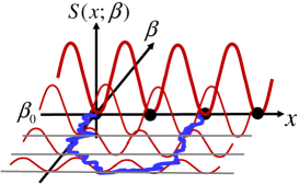
Figure 1: A random path in the extended configuration space $\mathcal{M}\times\mathcal{A}$. $\beta_{0}$ is the original value of $\beta$, at which the equilibrium distribution is highly multimodal in the $x$-direction.

We can also consider the coarse-graining of the extended configuration space. In [8], it is shown for the action (7) that the coarse-grained, extended configuration space $\bar{\mathcal{M}}\times\mathcal{A}$ has a geometry of Euclidean AdS_N+1 of the following form for large $\beta$:

$$ds^{2} \equiv d_{n}^{2}(X,X+dX)={\rm const.}\,\beta^{q}\,\sum_{i=1}^{N}dx_{i}^{2}+{\rm const.}\,\frac{d\beta^{2}}{\beta^{2}},$$ (8)

which can be transformed to a standard form, $ds^{2}\propto\rho^{2}\sum_{i=1}^{N}dx_{i}^{2}+d\rho^{2}/\rho^{2}\propto(\sum_{i=1}^{N}dx_{i}^{2}+dz^{2})/z^{2}$, by setting $\beta={\rm const.}\,\rho^{2/q}={\rm const.}\,z^{-2/q}$.

We comment that the discretization of $\mathcal{A}$ must be done so that configurations can move smoothly in the $\beta$-direction. A simple, geometrical analysis based on the distance shows that an exponential stepping is optimal for large $\beta$ [8, 12], and this result was used in the tempered Lefschetz thimble method [13, 14, 15, 16], that is a method towards solving the numerical sign problem.

3 Geometry for a stochastic process of matrices

3.1 $U(N)$ matrix model

The appearance of asymptotic AdS_N+1 metric may not be so much interesting as a model of gravity, because in quantum field theories, $x=(x_{i})$ corresponds to a configuration of field variables (such as a configuration of link variables on the lattice for the lattice gauge theory), and thus the degrees of freedom, $N$, is infinite in the thermodynamic limit. It is also hard to regard the configuration space as directly related to a spacetime.

However, things become different if we note that (7) is a one-body part of the $U(N)$ matrix model,

$$S(U;\beta)=\beta N\,{\rm Re}\,{\rm tr}\,(1-U)=\frac{\beta N}{2}\,{\rm tr}\,(2-U-U^{\dagger}),$$ (9)

with $U$ set to a diagonal form $U={\rm diag}\,[ix_{j}]$ $(j=1,\ldots,N)$, and if we recall that the eigenvalue can be regarded as a spacetime coordinate (see, e.g., [17]). To state this more precisely, we first rewrite the partition function as the integration over eigenvalues:

$$Z\equiv\int dU\,e^{-S(U;\beta)}\propto\int_{-\pi}^{\pi}\Bigl{(}\prod_{i=1}^{N}\frac{dx_{i}}{2\pi}\Bigr{)}\,\Bigl{(}\prod_{i<j}\sin^{2}\frac{x_{i}-x_{j}}{2}\Bigr{)}\,e^{-\beta N\,\sum_{i=1}^{N}(1-\cos x_{i})}.$$ (10)

The Faddeev-Popov determinant $\prod_{i<j}\sin^{2}(x_{i}-x_{j})/2$ gives a repulsive two-body potential between eigenvalues. Then, by introducing the collective coordinate $u$ through

$$\hat{\rho}(u)=\frac{1}{N}\,\sum_{i=1}^{N}\delta_{P}(x_{i}-u)~{}~{}(\mbox{$\delta_{P}(x)$: periodic delta function with period $2\pi$}),$$ (11)

we now can regard $u$ as a coordinate of a covering space with a period $2\pi m$, $\mathcal{M}=\{u|-\pi m\leq u<\pi m\}$.

It is known that the matrix model has a third-order phase transition in the large $N$ limit at the Gross-Witten-Wadia point $\beta=1$ [18, 19], where the functional form of the eigenvalue distribution $\rho(u)\equiv\lim_{N\to\infty}\langle\hat{\rho}(u)\rangle$ changes as follows ($x_{c}\equiv 2\arcsin(1/\sqrt{\beta})$):

• $\beta\geq 1$:

  $$\rho(u)=\left\{\begin{array}[]{cl}\dfrac{\beta}{\pi}\,\cos\dfrac{u}{2}\cdot\sqrt{\sin^{2}\dfrac{x_{c}}{2}-\sin^{2}\dfrac{u}{2}}&~{}~{}~{}(u\in I_{1})\\ 0&~{}~{}~{}(u\in I_{2})\end{array}\right.$$ (14)

• $\beta\leq 1$:

  $$\rho(u)=\frac{1}{2\pi}\,(1+\beta\cos u)~{}~{}~{}(\forall u),$$ (15)

where $I_{1}\equiv\{u\,|-x_{c}\leq[u]\leq x_{c}\}$ and $I_{2}\equiv\{u\,|-\pi\leq[u]\leq-x_{c}\,\,\mbox{or}+x_{c}\leq[u]<\pi\}$ with $[u]$ the projected value of $u$ to the fundamental region $[-\pi,\pi)$.

For a finite but large $N$, one-eigenvalue transitions yield an instanton effect of $e^{-O(N)}$ in the low-temperature phase ($\beta\geq 1$) [20] (see, e.g., [21, 22] for nonperturbative effects of the Gross-Witten-Wadia model). One can easily show that the one-eigenvalue feels the effective potential $S_{\rm eff}(u;\beta)=N\,v(u;\beta)+O(\ln N)$ with

$$v(u)\equiv\left\{\begin{array}[]{cl}0&(u\in I_{1})\\ 2\,\Bigl{|}\dfrac{\sin u/2}{\sin x_{c}/2}\Bigr{|}\,\sqrt{\dfrac{\sin^{2}u/2}{\sin^{2}x_{c}/2}-1}-2\,\ln\biggl{(}\Bigl{|}\dfrac{\sin u/2}{\sin x_{c}/2}\Bigr{|}+\sqrt{\dfrac{\sin^{2}u/2}{\sin^{2}x_{c}/2}-1}\biggr{)}&(u\in I_{2}).\end{array}\right.$$ (18)

The vanishing of potential in the region $|u|\leq x_{c}$ (we have set a possible additive constant to zero) can be understood as a balance between the one-body potential and the repulsive potential from other eigenvalues that are condensed with the distribution (14). Note that there is no such instanton effect for the high temperature phase, so that $v(u)$ vanishes for $\beta\leq 1$.

3.2 Geometry for a stochastic process of one-eigenvalue and a string theoretical interpretation

Let us consider the stochastic process of one-eigenvalue $u$ with respect to the effective action $S(u;\beta)=N\,v(u;\beta)+O(\ln N)$ for $\beta\geq 1$. The distance measures the difficulty of one-eigenvalue transitions in the background where other eigenvalues are condensed to large-$N$ solutions (14). We thus can interpret the distance as “measuring the background geometry of condensed eigenvalues by using the one-eigenvalue as a probe.” On the other hand, in noncritical string theory, one-eigenvalue corresponds to a D-instanton [23] (see also [24, 25, 26, 27, 28, 29]). Thus, the above can be rephrased as “measuring the background geometry by using a D-instanton as a probe.”

3.3 Emergence of a quantum blackhole

We now implement the simulated tempering by treating the inverse ’t Hooft coupling $\beta$ as a random variable. The coarse-grained, extended configuration space $\bar{\mathcal{M}}\times\mathcal{A}=\{X=(u,\beta)\}$ then becomes a two-dimensional lattice. Recall that we have set a periodic boundary condition for the $u$-direction with period $2\pi m$.

The geometry of $\bar{\mathcal{M}}\times\mathcal{A}$ in the low temperature phase ($\beta\geq 1$) should be as follows. First we recall that the effective potential disappears at $\beta=1$ in the large-$N$ limit, which means that the distance between $(0,\beta)$ and $(u,\beta)$ should become vanishingly small at $\beta=1$ for arbitrary $u$. Since we set a periodic boundary condition in the $u$-direction, we thus find that the $S^{1}$-cycle in the $u$-direction vanishes at $\beta=1$ in the large-$N$ limit (see the left panel of Fig. 2).

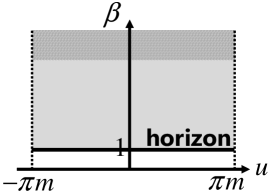
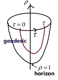
Figure 2: (Left) Geometry of $\bar{\mathcal{M}}\times\mathcal{A}$ in the large-$N$ limit. $u$ has a period $2\pi m$, and the $S^{1}$-cycle vanishes at the horizon $\beta=1$. (Right) The corresponding geometry in continuum. $\tau$ has a period $2\pi$, and the horizon is at $\rho=1$.

On the other hand, the effective action $S_{\rm eff}(u;\beta)=N\,v(u;\beta)+O(\ln N)$ has many local minima for $\beta\gg 1$, which means that the geometry of $\bar{\mathcal{M}}\times\mathcal{A}$ must be asymptotically AdS₂ for large $\beta$. Combining these two observations, we expect that the full geometry of $\bar{\mathcal{M}}\times\mathcal{A}$ for $\beta\geq 1$ is given by a Euclidean AdS₂ space with a horizon at the Gross-Witten-Wadia point, $\beta=1$. We choose a candidate metric in continuum of the form

$$ds^{2}=\ell^{2}\Bigl{[}(\rho^{2}-1)\,d\tau^{2}+\frac{d\rho^{2}}{\rho^{2}-1}\Bigr{]},$$ (19)

which is defined only for the outside of the horizon, $\rho\geq 1$ (see the right panel of Fig. 2). One can easily check that the metric (19) satisfies the equations $R_{\mu\nu}=\Lambda\,g_{\mu\nu}$ with $\Lambda=-1$ and has no conical singularity at the horizon $\rho=1$ when $\tau$ has a period $2\pi$. Furthermore, the geodesic distance $I(\tau,\rho)$ between two points $(0,\rho)$ and $(\tau,\rho)$ can be analytically calculated to be

$$I(\tau,\rho)=2\ell\,{\rm arccosh}\sqrt{\cos^{2}\frac{\tau}{2}+\rho^{2}\sin^{2}\frac{\tau}{2}}.$$ (20)

In the following discussions, we will set an ansatz that the two coordinate systems $(u,\beta)$ and $(\tau,\rho)$ are related to each other with a simple scaling:

$$u=m\tau,\quad\rho=\rho_{c}+\alpha(\beta-\beta_{c})^{q/2}.$$ (21)

3.4 Numerical confirmation

We now numerically confirm that the two geometries in Fig. 2 are the same under the relation (21), by comparing “the numerically obtained distances $d_{n}(X,Y)$ between $X=(0,\beta)$ and $Y=(u,\beta)$” with “the analytic values of distance, $I(\tau,\rho)$, between $(0,\rho)$ and $(\tau,\rho)$” for various $(u,\beta)$ with $u=u_{j}=2\pi j$ $(j=1,\ldots,25)$ and $\beta=\beta_{a}=5\times 5^{-a/5}$ $(a=0,1,\ldots,5)$.

With $N=20$, $n=200$ and $m=50$, we determine the parameters $(\ell,\beta_{c},\alpha,\rho_{c},q)$ by minimizing

$$\chi^{2}\equiv\sum_{j}\sum_{a}\Bigl{[}\frac{d_{n}^{2}((0,\beta_{a}),(u_{j},\beta_{a}))-I^{2}(\tau(u_{j}),\rho(\beta_{a}))}{\delta d_{n}^{2}((0,\beta_{a}),(u_{j},\beta_{a}))}\Bigr{]}^{2},$$ (22)

where $[\delta d_{n}^{2}(X,Y)]^{2}$ is a sample variance in the estimation of $d_{n}^{2}(X,Y)$. The obtained results are shown in Fig. 3 for the optimizing values,

$$\ell=0.10,~{}\beta_{c}=0.33,~{}\alpha=3.0,~{}\rho_{c}=0.93,~{}q=11$$ (23)

with $\sqrt{\chi^{2}/{\rm DOF}}=\sqrt{\chi^{2}/(25\times 6-5)}=1.6$, from which we confirm that the geometry of $\bar{\mathcal{M}}\times\mathcal{A}$ is well given by the metric (19) through the relation (21).

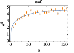
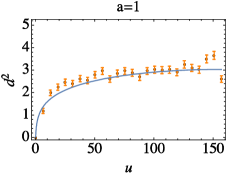
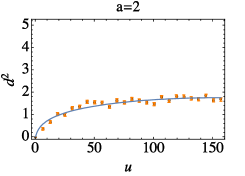
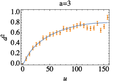
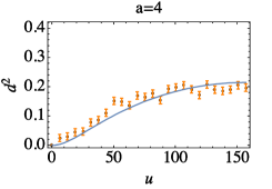
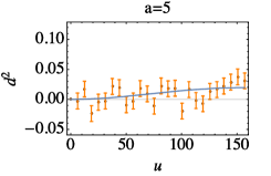
Figure 3: Numerically obtained squared distances $d_{n}^{2}(X,Y)$. The solid lines represent the squared geodesic distances, $I^{2}(\tau,\rho)$, for the optimizing parameters (3.11).

We comment that, for the optimizing parameters (23), the corresponding value of $\beta$ to the horizon $\rho=1$ is given by $\beta=0.83$. We expect that the discrepancy from the critical value $\beta=1$ can be understood as a finite $N$ correction (or it may imply that the relation (21) needs to be modified) [30].

4 Conclusion and outlook

In this article, we applied the distance between configurations, (4), to a Markov process of matrices. By identifying the eigenvalues with coordinates of a spacetime, this realizes a mechanism for the emergence of spacetime geometry from randomness. As an example, we showed that there emerges a Euclidean AdS geometry with a horizon from a tempered stochastic process of $U(N)$ matrix.

There are left many things we need to study in a more elaborate way. First of all, the fitting of the geometry with metric (19) is based on the assumption (21). It should be nice if we can analytically calculate the distance $d_{n}(X,Y)$ by using the tempered Langevin algorithm for the one-eigenvalue effective action $S_{\rm eff}(u;\beta)$. It should also be interesting to understand the results obtained here in the context of AdS/CFT correspondence, especially with a relation to the SYK model [31, 32] and the wormholes.

It must be important to generalize the present results to higher dimensions. We expect that an AdS_d+1 blackhole will emerge from a tempered stochastic process of the $d$-dimensional twisted Eguchi-Kawai model [33], where the action is given by $S(U_{\mu};\beta)=\beta\,{\rm Re}\,{\rm tr}\,(1-z_{\mu\nu}U_{\mu}U_{\nu}U_{\mu}^{\dagger}U_{\nu}^{\dagger})$ for $U_{\mu}\in U(N)$ $(\mu=1,\ldots,d)$. The spacetime coordinates $x=(x_{\mu})\in\mathbb{R}^{d}$ can be identified with the fluctuating modes corresponding to $U(1)^{d}$ transformations $U_{\mu}\to e^{i\,x_{\mu}}\,U_{\mu}$. For a symmetric twist, this $U(1)^{d}$ symmetry is actually broken at large $\beta$ if $N$ is taken to be sufficiently large [34]. In fact, as was also first found in [34], the $U(1)^{d}$ symmetry is restored step by step (the number of restored directions increases one by one as $\beta$ decreases). Since in our construction the spacetime can be extended only in the broken directions and the $S^{1}$-cycles vanish for the restored directions, we expect that an AdS_d+1 blackhole with a single horizon is obtained for the region $\beta\geq\beta_{H}$, where $\beta_{H}$ corresponds to the coupling at which a $U(1)$ symmetry is restored for the first time when reducing $\beta$ from a sufficiently large value.

As another direction of future project, it should be important to investigate whether we can find a stochastic process that gives de Sitter space. If such a process exists, then this should give a new mechanism to create an inflationary universe from randomness.

A study along these lines is now in progress and will be reported elsewhere.

References

- [1] E. Nelson, Derivation of the Schrödinger equation from Newtonian mechanics, Phys. Rev. 150 (1966) 1079.
- [2] G. Parisi and Y. s. Wu, Perturbation theory without gauge fixing, Sci. Sin. 24 (1981) 483.
- [3] C. D. Froggatt and H. B. Nielsen, Hierarchy of Quark Masses, Cabibbo Angles and CP Violation, Nucl. Phys. B 147 (1979) 277.
- [4] C. D. Froggatt and H. B. Nielsen, Standard model criticality prediction: Top mass GeV and Higgs mass GeV, Phys. Lett. B 368 (1996) 96 [hep-ph/9511371].
- [5] S. R. Coleman, Black Holes as Red Herrings: Topological Fluctuations and the Loss of Quantum Coherence, Nucl. Phys. B 307 (1988) 867.
- [6] S. R. Coleman, Why There Is Nothing Rather Than Something: A Theory of the Cosmological Constant, Nucl. Phys. B 310 (1988) 643.
- [7] M. Fukuma, N. Matsumoto and N. Umeda, Distance between configurations in Markov chain Monte Carlo simulations, JHEP 1712 (2017) 001 [arXiv:1705.06097 [hep-lat]].
- [8] M. Fukuma, N. Matsumoto and N. Umeda, Emergence of AdS geometry in the simulated tempering algorithm, JHEP 1811 (2018) 060 [arXiv:1806.10915 [hep-th]].
- [9] E. Marinari and G. Parisi, Simulated tempering: A New Monte Carlo scheme, Europhys. Lett. 19 (1992) 451 [hep-lat/9205018].
- [10] M. Lüscher, Trivializing maps, the Wilson flow and the HMC algorithm, Commun. Math. Phys. 293 (2010) 899 [arXiv:0907.5491 [hep-lat]].
- [11] M. Lüscher, Properties and uses of the Wilson flow in lattice QCD, JHEP 1008 (2010) 071, Erratum: [JHEP 1403 (2014) 092] [arXiv:1006.4518 [hep-lat]].
- [12] M. Fukuma, N. Matsumoto and N. Umeda, Distance between configurations in MCMC simulations and the geometrical optimization of the tempering algorithms, \posPoS(LATTICE2019)168 (2020) [arXiv:2001.02028 [hep-lat]].
- [13] M. Fukuma and N. Umeda, Parallel tempering algorithm for integration over Lefschetz thimbles, PTEP 2017 (2017) 073B01 [arXiv:1703.00861 [hep-lat]].
- [14] M. Fukuma, N. Matsumoto and N. Umeda, Applying the tempered Lefschetz thimble method to the Hubbard model away from half filling, Phys. Rev. D 100 (2019) 114510 arXiv:1906.04243 [cond-mat.str-el].
- [15] M. Fukuma, N. Matsumoto and N. Umeda, Implementation of the HMC algorithm on the tempered Lefschetz thimble method, arXiv:1912.13303 [hep-lat].
- [16] M. Fukuma, N. Matsumoto and N. Umeda, Tempered Lefschetz thimble method and its application to the Hubbard model away from half filling, in proceedings of Lattice 2019, \posPoS(LATTICE2019)090 (2020) [arXiv:2001.01665 [hep-lat]].
- [17] S. R. Das and A. Jevicki, String Field Theory and Physical Interpretation of Strings, Mod. Phys. Lett. A 5 (1990) 1639.
- [18] D. J. Gross and E. Witten, Possible Third Order Phase Transition in the Large N Lattice Gauge Theory, Phys. Rev. D 21 (1980) 446.
- [19] S. R. Wadia, Phase Transition in a Class of Exactly Soluble Model Lattice Gauge Theories, Phys. Lett. 93B (1980) 403.
- [20] F. David, Phases of the large- matrix model and non-perturbative effects in 2D gravity, Nucl. Phys. B 348 (1991) 507.
- [21] M. Marino, Nonperturbative effects and nonperturbative definitions in matrix models and topological strings, JHEP 0812 (2008) 114 [arXiv:0805.3033 [hep-th]].
- [22] A. Ahmed and G. V. Dunne, Transmutation of a Trans-series: The Gross-Witten-Wadia Phase Transition, JHEP 1711 (2017) 054 [arXiv:1710.01812 [hep-th]].
- [23] M. Fukuma and S. Yahikozawa, Comments on D instantons in strings, Phys. Lett. B 460 (1999) 71 [hep-th/9902169].
- [24] M. Fukuma and S. Yahikozawa, Nonperturbative effects in noncritical strings with soliton backgrounds, Phys. Lett. B 396 (1997) 97 [hep-th/9609210].
- [25] M. Fukuma and S. Yahikozawa, Combinatorics of solitons in noncritical string theory, Phys. Lett. B 393 (1997) 316 [hep-th/9610199].
- [26] M. Fukuma, H. Irie and S. Seki, Comments on the D-instanton calculus in (p,p+1) minimal string theory, Nucl. Phys. B 728 (2005) 67 [hep-th/0505253].
- [27] M. Fukuma, H. Irie and Y. Matsuo, Notes on the algebraic curves in (p,q) minimal string theory, JHEP 0609 (2006) 075 [hep-th/0602274].
- [28] M. Fukuma and H. Irie, A String field theoretical description of (p,q) minimal superstrings, JHEP 0701 (2007) 037 [hep-th/0611045].
- [29] M. Fukuma and H. Irie, Supermatrix models and multi ZZ-brane partition functions in minimal superstring theories, JHEP 0703 (2007) 101 [hep-th/0701031].
- [30] M. Fukuma and N. Matsumoto, work in progress.
- [31] S. Sachdev and J. Ye, Gapless spin fluid ground state in a random, quantum Heisenberg magnet, Phys. Rev. Lett. 70 (1993) 3339 [cond-mat/9212030].
- [32] A. Kitaev, A simple model of quantum holography, KITP strings seminar and Entanglement 2015 program (2015), http://online.kitp.ucsb.edu/online/entangled15/
- [33] A. Gonzalez-Arroyo and M. Okawa, Twisted-Eguchi-Kawai model: A reduced model for large- lattice gauge theory, Phys. Rev. D 27 (1983) 2397.
- [34] M. Teper and H. Vairinhos, Symmetry breaking in twisted Eguchi-Kawai models, Phys. Lett. B 652 (2007) 359 [hep-th/0612097].