Deep-n-Cheap: An Automated Search Framework for Low Complexity Deep Learning

Abstract

We present Deep-n-Cheap – an open-source AutoML framework to search for deep learning models. This search includes both architecture and training hyperparameters, and supports convolutional neural networks and multi-layer perceptrons. Our framework is targeted for deployment on both benchmark and custom datasets, and as a result, offers a greater degree of search space customizability as compared to a more limited search over only pre-existing models from literature. We also introduce the technique of ‘search transfer’, which demonstrates the generalization capabilities of the models found by our framework to multiple datasets.

Deep-n-Cheap includes a user-customizable complexity penalty which trades off performance with training time or number of parameters. Specifically, our framework results in models offering performance comparable to state-of-the-art while taking 1-2 orders of magnitude less time to train than models from other AutoML and model search frameworks. Additionally, this work investigates and develops various insights regarding the search process. In particular, we show the superiority of a greedy strategy and justify our choice of Bayesian optimization as the primary search methodology over random / grid search.

1 Introduction

Artificial neural networks in deep learning systems are critical drivers of emerging technologies such as computer vision, text classification, and autonomous applications. In particular, convolutional neural networks are used for image related tasks while multilayer perceptrons can be used for general purpose classification tasks. Manually designing these NNs is challenging since they typically have a large number of interconnected layers [18, 33] and require a large number of decisions to be made regarding hyperparameters. These hyperparameters, as opposed to trainable parameters like weights and biases, are not learned by the network. They need to be specified and adjusted by an external entity, i.e., the designer. They can be broadly grouped into two categories – a) architectural hyperparameters, such as the type of each layer and the number of nodes in it, and b) training hyperparameters, such as the learning rate and batch size. The difficulty of manually designing hyperparameters to find a good NN is exacerbated by the fact that several hyperparameters interact with each other to have a combined effect on the final performance.

1.0.1 Motivation and Related Work:

The problem of searching for good NNs has resulted in several efforts towards automating this process. These efforts include AutoML frameworks such as Auto-Keras [16], AutoGluon [2] and Auto-PyTorch [22], which are open source software packages applicable to a variety of tasks and types of NNs. The major focus of these efforts is on providing user-friendly toolkits to search for good hyperparameter values.

Several other efforts place more emphasis on novel techniques for the search process. These can be broadly grouped into Neural Architecture Search (NAS) efforts such as [25, 20, 19, 3, 23, 26, 32, 30, 9, 12], and efforts that place a larger emphasis on training hyperparameters over architecture [8, 28, 6, 31]. An alternate grouping is on the basis of search methodology – a) reinforcement learning [25, 34, 3], b) evolution / genetic operations [23, 26, 32], and c) Bayesian Optimization [17, 31, 28, 29]. Although the efforts described in this paragraph often come with publicly available software, they are typically not intended for general purpose use, e.g., the code release for [9] only allows reproducing NNs on two datasets. This differentiates them from AutoML frameworks.

Deep NNs often suffer from complexity bottlenecks – either in storage, quantified by the total number of trainable parameters $N_{p}$, or computational, such as the number of FLOPs or the time taken to perform training and/or inference. Prior efforts on NN search penalize inference complexity in specific ways – latency in [9], FLOPs in [30], and both in [12]. However, inference complexity is significantly different from training since the latter includes backpropagation and parameter updates every batch. For example, the resulting network for CIFAR-10 in [9] takes a minute to perform inference, but hours to train. Moreover, while there is considerable interest in popular benchmark datasets, in most real-world applications deep learning models need to be trained on custom datasets for which readymade, pre-trained models do not exist [21, 5, 27]. This leads to an increasing number of resource-constrained devices needing to perform training on the fly, e.g., self-driving cars.

The computing platform is also important, e.g., changing batch size has a greater effect on training time per epoch on GPU than CPU. Therefore, calculating the FLOP count is not always an accurate measure of the time and resources expended in training a NN. Some previous works have proposed pre-defined sparsity [10, 11] and stochastic depth [13] to reduce training time, while [24] focuses on finding the quickest training time to get to a certain level of performance. Note that these are all manual methods, not search frameworks.

1.0.2 Overview and Contributions:

This paper introduces Deep-n-Cheap (DnC) – an open-source AutoML framework to search for deep learning models. We specifically target the training complexity bottleneck by including a penalty for training time per epoch $t_{\text{tr}}$ in our search objective. The penalty coefficient can be varied by the user to obtain a family of networks trading off performance and complexity. Additionally, we also support storage complexity penalties for $N_{p}$.

DnC searches for both architecture and training hyperparameters. While the architecture search derives some ideas from literature, we have striven to offer the user a considerable amount of customizability in specifying the search space. This is important for training on custom datasets which can have significantly different requirements than those associated with benchmark datasets.

DnC primarily uses Bayesian Optimization (BO) and currently supports classification tasks using CNNs and MLPs. A notable aspect is search transfer, where we found that the best NNs obtained from searching over one dataset give good performance on a different dataset. This helps to improve generalization in NNs – such as on custom datasets – instead of purely optimizing for specific problems.

The following are the key contributions of this paper:

1. Complexity: To the best of our knowledge, DnC is the only AutoML framework targeting training complexity reduction. We show results on several datasets on both GPU and CPU. Our models achieve performance comparable to state-of-the-art, with training times that are 1-2 orders of magnitude less than those for models obtained from other AutoML and search efforts.

2. Usability: DnC offers a highly customizable three-stage search interface for both architecture and training hyperparameters. As opposed to Auto-Keras and AutoGluon, our search includes a) batch size that affects training times, and b) architectures beyond pre-existing ones found in literature. As a result, our target users include those who want to train quickly on custom datasets. As an example, our framework achieves the highest performance and lowest training times on the custom Reuters RCV1 dataset [10]. We also introduce search transfer to explore generalization capabilities of architectures to multiple datasets under different training hyperparameter settings.

3. Insights: We conduct investigations into the search process and draw several insights that will help guide a deeper understanding of NNs and search methodologies. We introduce a new similarity measure for BO and a new distance function for NNs. We empirically justify the value of our greedy three-stage search approach over less greedy approaches, and the superiority of BO over random and grid search.

The paper is structured as follows –– Sec. 2 outlines our search methodology, Sec. 3 our experimental results, Sec. 4 includes additional investigations and insights, Sec. 5 compares with related work, and Sec. 6 concludes the paper.

2 Our Approach

Given a dataset, our framework searches for NN configurations through sequential stages in multiple search spaces. Each config is trained for the same number of epochs, e.g., 100. There have been works on extrapolating NN performance from limited training [4, 19], however we train for a large number of epochs to predict with significant confidence the final performance of a NN after convergence. Configs are mapped to objective values using: c f(Config) = f_p(Config) + w_cf_c(Config) where $w_{c}$ controls the importance given to the complexity term. The goal of the search is to minimize $f$. Its components are: rCl f_p &= 1 - Best Validation Accuracy
f_c = cc0 where $c$ is the complexity metric for the current config (either $t_{\text{tr}}$ or $N_{p}$), and $c_{0}$ is a reference value for the same metric (typically obtained for a high complexity config in the space). Lower values of $w_{c}$ focus more on performance, i.e., improving accuracy. One key contribution of this work is characterizing higher values of $w_{c}$ that lead to reduced complexity NNs that train fast – these also reduce the search cost by speeding up the overall search process.

2.1 Three-stage search process

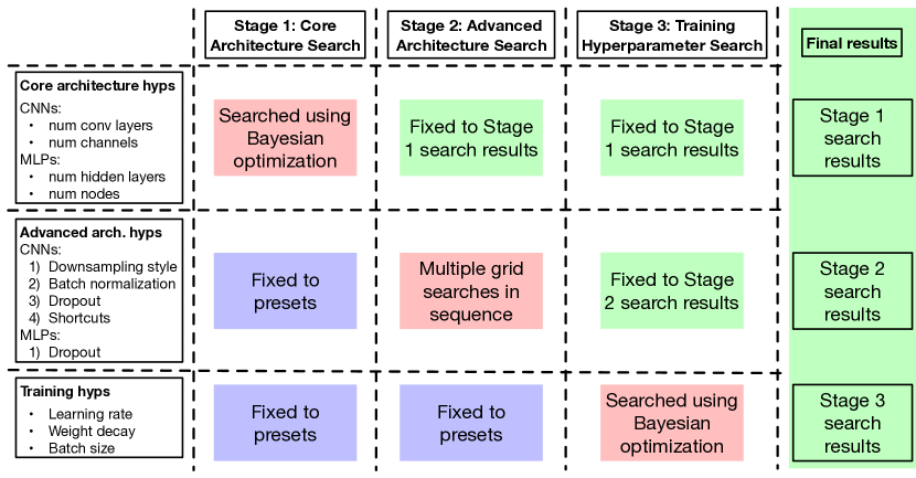
Figure 1: Three-stage search process for DnC.

2.1.1 Stage 1 – Core architecture search:

For CNNs, the combined search space consists of the number of convolutional (conv) layers and number of channels in each, while for MLPs, it is the number of hidden layers and number of nodes in each. Other architectural hyperparameters such as batch normalization (BN) and dropout layers and all training hyperparameters are fixed to presets that we found to work well across a variety of datasets and network depths. BO is used to minimize $f$ and the corresponding best config is the Stage 1 result.

2.1.2 Stage 2 – Advanced architecture search:

This stage starts from the resulting architecture from Stage 1 and uses grid search to search for the following CNN hyperparameters through a sequence of sub-stages – 1) whether to use strides or max pooling layers for downsampling, 2) amount of BN layers, 3) amount of dropout layers and drop probabilities, and 4) amount of shortcut connections. This is not a combined space, instead grid search first picks the downsampling choice leading to the minimum $f$ value, then freezes that and searches over BN, and so on. This ordering yielded good empirical results, however, reordering is supported by the framework. For MLPs, there is a single grid search for dropout probabilities. As in the previous stage, training hyperparameters are fixed to presets. The result from Stage 2 is the result from the final sub-stage.

2.1.3 Stage 3 – Training hyperparameter search:

The architecture is finalized after Stage 2. In Stage 3 – identical for CNNs and MLPs – we search over the combined space of initial learning rate $\eta$, weight decay $\lambda$ and batch size, using BO to minimize $f$. The final config after Stage 3 comprises both architecture and training hyperparameters. The complete process is summarized in Fig. 1.

2.2 Bayesian Optimization

Bayesian Optimization is useful for optimizing functions that are black-box and/or expensive to evaluate such as $f$, which requires NN training. The initial step when performing BO is to sample $n_{1}$ configs from the search space, $\{\bm{x}_{1},\allowbreak\cdots,\allowbreak\bm{x}_{n_{1}}\}$, calculate their corresponding objective values, $\{f\left(\bm{x}_{1}\right),\allowbreak\cdots,\allowbreak f\left(\bm{x}_{n_{1}}\right)\}$, and form a Gaussian prior. The mean vector $\bm{\mu}$ is filled with the mean of the $f$ values, and covariance matrix $\bm{\Sigma}$ is such that $\Sigma_{ij}=\sigma\left(\bm{x}_{i},\bm{x}_{j}\right)$, where $\sigma(\cdot,\cdot)$ is a kernel function that takes a high value $\in[0,1]$ if configs $\bm{x}_{i}$ and $\bm{x}_{j}$ are similar.

Then the algorithm continues for $n_{2}$ steps, each step consisting of sampling $n_{3}$ configs, picking the config with the maximum expected improvement, computing its $f$ value, and updating $\bm{\mu}$ and $\bm{\Sigma}$ accordingly. The reader is referred to [7] for a complete tutorial on BO – where eq. (4) in particular has details of expected improvement. Note that BO explores a total of $n_{1}+n_{2}n_{3}$ states in the search space, but the expensive $f$ computation only occurs for $n_{1}+n_{2}$ states.

2.2.1 Similarity between NN configurations:

We begin by defining the distance between values of a particular hyperparameter $k$ for two configs $\bm{x}_{i}$ and $\bm{x}_{j}$. Larger distances denote dissimilarity. We initially considered the distance functions defined in Sections 2 and 3 of [14], but then adopted an alternate one that resulted in similar performance with less tuning. We call it the ramp distance: c d(x_ik,x_jk) = ω_k (—xik-xjk—uk-lk)^r_k where $u_{k}$ and $l_{k}$ are respectively the upper and lower bounds for $k$, $\omega_{k}$ is a scaling coefficient, and $r_{k}$ is a fractional power used for stretching small differences. Note that $d$ is 0 when $x_{ik}=x_{jk}$, and reaches a maximum of $\omega_{k}$ when they are the furthest apart. $x_{ik}$ and $x_{jk}$ are computed in different ways depending on $k$:

• If $k$ is batch size or number of layers, $x_{ik}$ and $x_{jk}$ are the actual values.

• If $k$ is $\eta$ or $\lambda$, $x_{ik}$ and $x_{jk}$ are the logarithms of the actual values.

• When $k$ is the hidden node configuration of a MLP, we sum the nodes together across all hidden layers. This is because we found that the sum has a greater impact on $f$ than considering layers individually, e.g., a config with three 300-node hidden layers has a closer $f$ value to a config with one 1000-node hidden layer than a config with three 100-node hidden layers.

• When $k$ is the conv channel configuration of a CNN, we calculate individual distances for each layer. If the number of layers is different, the distance is maximum for each of the extra layers, i.e., $\omega$. This idea is inspired from [14], as compared to alternative similarity measures in [17, 16]. We follow this layer-by-layer comparison because our prior experiments showed that the representations learned by a certain conv layer in a CNN are similar to those learned by layers at the same depth in different CNNs. Additionally, this approach performed better than the summing across layers as in MLPs.

Each individual distance $d\left(x_{ik},x_{jk}\right)$ is converted to its kernel value $\sigma\left(x_{ik},x_{jk}\right)$ using the squared exponential function, then we take their convex combination for all $K$ hyperparameters using coefficients $\left\{s_{k}\right\}$ to finally get $\sigma\left(\bm{x}_{i},\bm{x}_{j}\right)$. An example is given in Fig. 2. rCl σ(x_ik,x_jk) &= exp(-d2(xik, xjk)2 )
σ(x_i,x_j) = ∑_k=1^Ks_kσ(x_ik,x_jk)

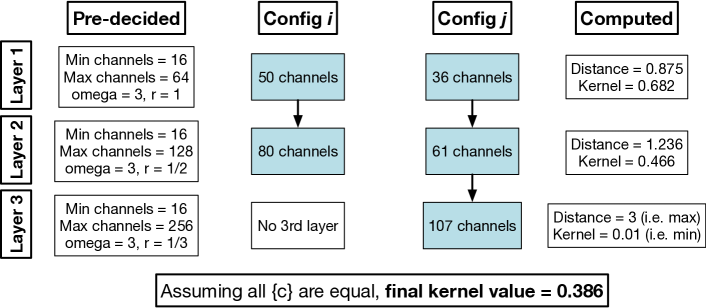
Figure 2: Calculating Stage 1 similarity for two conv channel configs: $\bm{x}_{i}=[50,\allowbreak 80]$ and $\bm{x}_{j}=[36,\allowbreak 61,\allowbreak 107]$. Taking the 1st conv layer as an example, the pre-decided values are $u_{1}=64$, $l_{1}=16$, $\omega_{1}=3$ and $r_{1}=1$ (more details on these choices in Sec. 3). The distance is $d_{1}=3\times\left[(50-36)/(64-16)\right]^{1}=0.875$, and kernel value is $\sigma_{1}=\exp\left(-0.5\times 0.875^{2}\right)=0.682$. Similarly we get $\sigma_{2}=0.466$ and $\sigma_{3}=0.01$ (note that $d_{3}=\omega_{3}$ due to the absence of the 3rd layer in $\bm{x}_{i}$). Combining these using $s_{1}=s_{2}=s_{3}=\nicefrac{{1}}{{3}}$ yields $\sigma\left(\bm{x}_{i},\bm{x}_{j}\right)=0.386$.

3 Experimental Results

This section presents results of our search framework on different datasets for both CNN and MLP classification problems, along with the search settings used. Note that most of these settings can be customized by the user – this leads to one of our key contributions of using limited knowledge from literature to enable wider exploration of NNs for various custom problems. We used the Pytorch library on two platforms: a) GPU – an Amazon Web Services p3.2xlarge instance that uses a single NVIDIA V100 GPU with 16 GB memory and 8 vCPUs, and b) CPU – a mid-2014 Macbook Pro CPU with 2.2 GHz Intel Core i7 processor and 16GB 1.6 GHz DDR3 RAM. For BO, we used $n_{1}=n_{2}=15$ and $n_{3}=1000$.

3.1 CNNs

All CNN experiments are on GPU. The datasets used are CIFAR-10 and -100 with train-validation-test splits of 40k-10k-10k, and Fashion MNIST (FMNIST) with 50k-10k-10k. Standard augmentation is always used – channel-wise normalization, random crops from 4 pixel padding on each side, and random horizontal flips. Augmentation requires Pytorch data loaders that incur timing overheads, so we also show results on unaugmented CIFAR-10 where the whole dataset is loaded into memory at the beginning and $t_{\text{tr}}$ reduces as a result.

For Stage 1, we use BO to search over CNNs with 4–16 conv layers, the first of which has $c_{1}\in\{16,\allowbreak 17,\allowbreak\cdots,\allowbreak 64\}$ channels and each subsequent layer has $c_{i+1}\in\{c_{i},\allowbreak c_{i}+1,\allowbreak\cdots,\allowbreak\min\left(2c_{i},512\right)\}$ channels. We allow the number of channels in a layer to have arbitrary integer values, not just fixed to multiples of 8. Kernel sizes are fixed to 3x3. Downsampling precedes layers where $c_{i}$ crosses 64, 128 and 256 (this is due to GPU memory limitations). During Stage 1, all conv layers are followed by BN and dropout with $30\%$ drop probability. Configs with more than 8 conv layers have shortcut connections. Global average pooling and a softmax classifier follows the conv portion. There are no hidden classifier layers since we empirically obtained no performance benefit. For both Stages 1 and 2, we used the default Adam optimizer with $\eta=10^{-3}$, decayed by $80\%$ at the half and three-quarter points of training, batch size of 256, and $\lambda=\mathbb{I}(N_{p}\geq 10^{6})\times N_{p}/10^{11}$, $\mathbb{I}$ being the indicator function. We empirically found this rule to work well.

For Stage 2, the first grid search is over all possible combinations of using either strides or max pooling for the downsampling layers. Second, we vary the fraction of BN layers through $\left[0,\nicefrac{{1}}{{4}},\nicefrac{{1}}{{2}},\nicefrac{{3}}{{4}}\right]$. For example, if there are 7 conv layers, a setting of $\nicefrac{{1}}{{2}}$ will place BN layers after conv layers 2, 4, 6 and 7. Third, we vary the fraction of dropout layers in a manner similar to BN, and drop probabilities over $[0.1,0.2]$ for the input layer and $[0.15,0.3,0.45]$ for all other layers. Finally, we search over shortcut connections – none, every 4th layer, or every other layer. Note that any shortcut connection skips over 2 layers.

For Stage 3, we used BO to search over a) $\eta\in\left\{10^{x}\right\}$ for $x\in[1,5]$, b) $\lambda\in\left\{10^{x}\right\}$ for $x\in[-6,-3]$, with $\lambda$ converted to $0$ when $x<-5$, and c) batch sizes in $[32,\allowbreak 33,\allowbreak\cdots,\allowbreak 512]$. We found that batch sizes that are not powers of 2 did not lead to any slowdown on the platforms used.

The penalty function $f_{c}$ uses normalized $t_{\text{tr}}$, since this is the major bottleneck in developing CNNs. Each config was trained for 100 epochs on the train set and evaluated on the validation set to obtain $f_{p}$. We ran experiments for 5 different values of $w_{c}$: $[0,0.01,0.1,1,10]$. The best network from each search was then trained on the combined training and validation set, and evaluated on the test set for 300 epochs to get final test accuracies and $t_{\text{tr}}$ values.

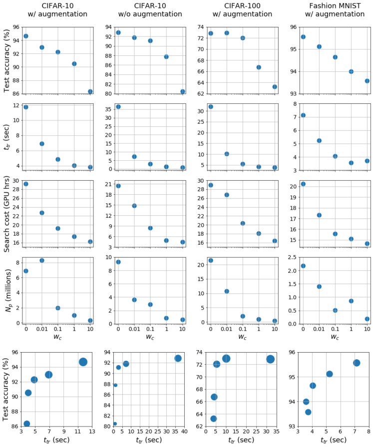
Figure 3: Characterizing a family of NNs for CIFAR-10 augmented (1st column), unaugmented (2nd column), CIFAR-100 augmented (3rd column) and FMNIST augmented (4th column), obtained from DnC for different $w_{c}$. We plot test accuracy in 300 epochs (1st row), $t_{\text{tr}}$ on combined train and validation sets (2nd row), search cost (3rd row) and $N_{p}$ (4th row), all against $w_{c}$. The 5th row shows the performance-complexity tradeoff, with dot size proportional to search cost.

As shown in Fig. 3, we obtain a family of networks by varying $w_{c}$. Performance in the form of test accuracy trades off with complexity in the form of $t_{\text{tr}}$. The latter is correlated with search cost and $N_{p}$. The last row of figures directly plot the performance-complexity tradeoff. These curves rise sharply towards the left and flatten out towards the right, indicating diminishing performance returns as complexity is increased. This highlights one of our key contributions – allowing the user to choose fast training NNs that perform well.

Taking augmented CIFAR-10 as an example, DnC found the following best config for $w_{c}=0$: 14 conv layers with $\{c\}=(50,\allowbreak 52,\allowbreak 53,\allowbreak 59,\allowbreak 95,\allowbreak 96,\allowbreak 97,\allowbreak 120,\allowbreak 193,\allowbreak 239,\allowbreak 351,\allowbreak 385,\allowbreak 488,\allowbreak 496)$, the 4th layer has a stride of 2 while max pooling follows layers 8 and 10, BN follows all conv layers, dropout with drop probability $0.3$ follows every other conv block, and skip connections are present for every other conv block. The best found $\eta$ remains $10^{-3}$, batch size is 120 and $\lambda=3.35\times 10^{-5}$. We note that we achieve good performance with a NN that has irregular $\{c\}$ values and is also not very deep – the latter is consistent with the findings in [33]. Also note that the best config found for $w_{c}=10$ only has 4 conv layers.

3.2 MLPs

We ran CPU experiments on the MNIST and FMNIST datasets in permutation-invariant format (i.e., images are flattened to a single layer of 784 input pixels) without any augmentation, and GPU experiments on the Reuters RCV1 dataset constructed as given in [10]. Each dataset is loaded into memory in its entirety, eliminating data loader overheads.

For Stage 1, we search over 0–2 hidden layers for MNIST and FMNIST, number of nodes in each being 20–400. These numbers change for RCV1 to 0–3 and 50–1000 since it is a larger dataset. Every layer is followed by a dropout layer with $20\%$ drop probability. Training hyperparameters are fixed as in the case of CNNs, with the difference that $\lambda=\mathbb{I}(N_{p}\geq 10^{4})\times N_{p}/10^{9}$ for MNIST and FMNIST and $\lambda=\mathbb{I}(N_{p}\geq 10^{5})\times N_{p}/10^{10}$ for RCV1. For Stage 2, we do a grid search over drop probabilities in $[0,0.1,0.3,0.4,0.5]$, and for Stage 3, the training hyperparameter search is identical to CNNs.

We ran separate searches for individual penalty functions – normalized $t_{\text{tr}}$ and normalized $N_{p}$. The latter is owing to the fact that MLPs often massively increase the number of parameters and thereby storage complexity of NNs [18]. The train-validation-test splits for MNIST and FMNIST are 50k-10k-10k, and 178k-50k-100k for RCV1. Candidate networks were trained for 60 epochs and the final networks tested after 180 epochs. As before, $w_{c}\in[0,0.01,0.1,1,10]$ for MNIST and FMNIST. For RCV1, the results for $w_{c}=10$ were mostly similar to $w_{c}=1$, so we replace $10$ with $0.03$. The plots against $w_{c}$ are shown in Fig. 4, where pink dots are for $t_{\text{tr}}$ penalty and black crosses are for $N_{p}$ penalty.

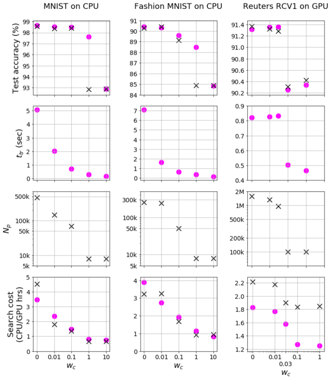
Figure 4: Characterizing a family of NNs for MNIST (1st column) and FMNIST (2nd column) on CPU, and RCV1 (3rd column) on GPU, obtained from DnC for different $w_{c}$. We plot test accuracy in 180 epochs (1st row), $t_{\text{tr}}$ on combined train and validation sets (2nd row), $N_{p}$ (3rd row), and search cost (4th row), all against $w_{c}$. The search penalty is $t_{\text{tr}}$ for the pink dots and $N_{p}$ for the black crosses.

The trends in Fig. 4 are qualitatively similar to those in Fig. 3. When penalizing $N_{p}$, the two lowest complexity networks in each case have no hidden layers, so they both have exactly the same $N_{p}$ (results differ due to different training hyperparameters). Of interest is the subfigure on the bottom right, indicating much longer search times when penalizing $N_{p}$ as compared to $t_{\text{tr}}$. This is because time is not a factor when penalizing $N_{p}$, so the search picks smaller batch sizes that increase $t_{\text{tr}}$ with a view to improving performance. Interestingly enough, this does not actually lead to performance benefit as shown in the subfigure on the top-right, where the black crosses occupy similar locations as the pink dots.

4 Investigations and insights

4.1 Search transfer

One goal of our search framework is to find models that are applicable to a wide variety of problems and datasets suited to different user requirements. To evaluate this aspect, we experimented on whether a NN architecture found from searching through Stages 1 and 2 on dataset A can be applied to dataset B after searching for Stage 3 on it. In other words, how does transferring an architecture compare to ‘native’ configs, i.e., those searched for through all three stages on dataset B. This process is shown on the left in Fig. 5. Note that we repeat Stage 3 of the search since it optimizes training hyperparameters such as weight decay, which are related to the capacity of the network to learn a new dataset. This is contrary to simply transferring the architecture as in [34].

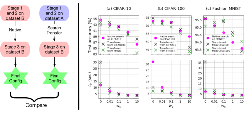
Figure 5: Left: Process of search transfer – comparing configs obtained from native search with those where Stage 3 is done on a dataset different from Stages 1 and 2. Right: Results of CNN search transfer to (a) CIFAR-10, (b) CIFAR-100, (c) FMNIST. All datasets are augmented. Pink dots denote native search.

We took the best CNN architectures found from searches on CIFAR-10, CIFAR-100 and FMNIST (as depicted in Fig. 3) and transferred them to each other for Stage 3 searching. The results for test accuracy and $t_{\text{tr}}$ are shown on the right in Fig. 5. We note that the architectures generally transfer well. In particular, transferring from FMNIST (green crosses in subfigures (a) and (b)) results in slight performance degradation since those architectures have $N_{p}$ around 1M-2M, while some architectures found from native searches (pink dots) on CIFAR have $N_{p}>20$M. However, architectures transferred between CIFAR-10 and -100 often exceed native performance. Moreover, almost all the architectures transferred from CIFAR-100 (green crosses in subfigure (c)) exceed native performance on FMNIST, which again is likely due to bigger $N_{p}$. We also note that $t_{\text{tr}}$ values remain very similar on transferring, except for the $w_{c}=0$ case where there is absolutely no time penalty.

4.2 Greedy strategy

Our search methodology is greedy in the sense that it preserves only the best config resulting in the minimum $f$ value from each stage and sub-stage. We also experimented with a non-greedy strategy. Instead of one, we picked the three best configs from Stage 1 – $\left\{\bm{x}_{1},\bm{x}_{2},\bm{x}_{3}\right\}$, then ran separate grid searches on each of them to get three corresponding configs at the end of Stage 2, and finally picked the three best configs for each of their Stage 3 runs for a total of nine different configs – $\left\{\bm{x}_{11},\bm{x}_{12},\bm{x}_{13},\bm{x}_{21},\cdots,\bm{x}_{33}\right\}$. Following a purely greedy approach would have resulted in only $\bm{x}_{11}$, while following a greedy approach for Stages 1 and 2 but not Stage 3 would have resulted in $\left\{\bm{x}_{11},\bm{x}_{12},\bm{x}_{13}\right\}$. We plotted the losses for each config for five different values of $w_{c}$ on CIFAR-10 unaugmented (Fig. 6 shows three of these). In each case we found that following a purely greedy approach yielded best results, which justifies our choice for DnC.

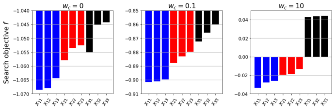
Figure 6: Search objective values (lower the better) for three best configs from Stage 1 (blue, red, black), optimized through Stages 2 and 3 and three best configs chosen for each in Stage 3. Results shown for different $w_{c}$ on CIFAR-10 unaugmented.

4.3 Bayesian optimization vs random and grid search

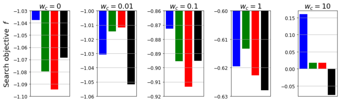
Figure 7: Search objective values (lower the better) for purely random search (30 samples, blue) vs purely grid search via Sobol sequencing (30 samples, green) vs balanced BO (15 initial samples, 15 optimized samples, red) vs extreme BO (1 initial sample, 29 optimized samples, black). Results shown for different $w_{c}$ on CIFAR-10 unaugmented.

We use Sobol sequencing – a space-filling method that selects points similar to grid search – to select initial points from the search space and construct the BO prior. We experimented on the usefulness of BO by comparing the final search loss $f$ achieved by performing the Stage 1 and 3 searches in four different ways:

• Random search: pick 30 prior points randomly, no optimization steps

• Grid search: pick 30 prior points via Sobol sequencing, no optimization steps

• Balanced BO (DnC default): pick 15 prior points via Sobol sequencing, 15 optimization steps

• Extreme BO: pick 1 initial point, 29 optimization steps

The results in Fig. 7 are for different $w_{c}$ on CIFAR-10. BO outperforms random and grid search on each occasion. In particular, more optimization steps are beneficial for low complexity models, while the advantages of BO are not significant for high performing models. We believe that this is due to the fact that many deep nets [33] are fairly robust to training hyperparameter settings.

5 Comparison to related work

Table 1: Comparison of features of AutoML frameworks

Framework	Architecture search space	Training	Adjust model
		hyp search	complexity
Auto-Keras	Only pre-existing architectures	No	No
AutoGluon	Only pre-existing architectures	Yes	No
Auto-PyTorch	Customizable by user	Yes	No
Deep-n-Cheap	Customizable by user	Yes	Penalize $t_{\text{tr}}$, $N_{p}$

Table 1 compares features of different AutoML frameworks. To the best of our knowledge, only DnC allows the user to specifically penalize complexity of the resulting models. This allows our framework to find models with performance comparable to other state-of-the-art methods, while significantly reducing the computational burden of training. This is shown in Table 2, which compares the search process and metrics of the final model found for CNNs on CIFAR-10, and Table 3, which does the same for MLPs on FMNIST and RCV1 for DnC and Auto-PyTorch only, since Auto-Keras and AutoGluon do not have explicit support for MLPs at the time of writing.

Note that Auto-Keras and AutoGluon do not support explicitly obtaining the final model from the search, which is needed to perform separate inference on the test set after the search. As a result, in order to have a fair comparison, Tables 2 and 3 use metrics from the search process – $t_{\text{tr}}$ is for the train set and the performance metric is best validation accuracy. These are reported for the best model found from each search. Auto-Keras and AutoGluon use fixed batch sizes across all models, however, Auto-PyTorch and DnC also do a search over batch sizes. We have included batch size since it affects $t_{\text{tr}}$. Each config for each search is run for the same number of epochs, as described in Sec. 3. The exception is Auto-PyTorch, where a key feature is variable number of epochs.

Table 2: Comparing frameworks on CNNs for CIFAR-10 augmented on GPU

Framework	Additional	Search cost	Best model found from search
	settings	(GPU hrs)	Architecture	$t_{\text{tr}}$ (sec)	Batch size	Best val acc ($\%$)
Proxyless NAS	Proxyless-G	96	537 conv layers	429	64	93.22
Auto-Keras	Default run	14.33	Resnet-20 v2	33	32	74.89
AutoGluon	Default run	3	Resnet-20 v1	37	64	88.6
	Extended run	101	Resnet-56 v1	46	64	91.22
Auto-Pytorch	‘tiny cs’	6.17	30 conv layers	39	64	87.81
	‘full cs’	6.13	41 conv layers	31	106	86.37
Deep-n-Cheap	$w_{c}=0$	29.17	14 conv layers	10	120	93.74
	$w_{c}=0.1$	19.23	8 conv layers	4	459	91.89
	$w_{c}=10$	16.23	4 conv layers	3	256	83.82

Table 3: Comparing AutoML frameworks on MLPs for FMNIST and RCV1 on GPU

Framework	Additional	Search cost	Best model found from search
	settings	(GPU hrs)	MLP layers	$N_{p}$	$t_{\text{tr}}$ (sec)	Batch size	Best val acc ($\%$)
Fashion MNIST
Auto-Pytorch	‘tiny cs’	6.76	50	27.8M	19.2	125	91
	‘medium cs’	5.53	20	3.5M	8.3	184	90.52
	‘full cs’	6.63	12	122k	5.4	173	90.61
Deep-n-Cheap	$w_{c}=0$	0.52	3	263k	0.4	272	90.24
(penalize $t_{\text{tr}}$)	$w_{c}=10$	0.3	1	7.9k	0.1	511	84.39
Deep-n-Cheap	$w_{c}=0$	0.44	2	317k	0.5	153	90.53
(penalize $N_{p}$)	$w_{c}=10$	0.4	1	7.9k	0.2	256	86.06
Reuters RCV1
Auto-Pytorch	‘tiny cs’	7.22	38	19.7M	39.6	125	88.91
	‘medium cs’	6.47	11	11.2M	22.3	337	90.77
Deep-n-Cheap	$w_{c}=0$	1.83	2	1.32M	0.7	503	91.36
(penalize $t_{\text{tr}}$)	$w_{c}=1$	1.25	1	100k	0.4	512	90.34
Deep-n-Cheap	$w_{c}=0$	2.22	2	1.6M	0.6	512	91.36
(penalize $N_{p}$)	$w_{c}=1$	1.85	1	100k	5.54	33	90.4

We note that for CNNs, DnC results in both the fastest $t_{\text{tr}}$ and highest performance. The performance of Proxyless NAS is comparable, while taking 43X more time to train. This highlights one of our key features – the ability to find models with performance comparable to state-of-the-art while massively reducing training complexity. The search cost is lowest for the default AutoGluon run, which only runs 3 configs. We also did an extended run for $\sim 100$ models on AutoGluon to make it match with DnC and Auto-Keras – this results in the longest search time without significant performance gain.

For MLPs, DnC has the fastest search times and lowest $t_{\text{tr}}$ and $N_{p}$ values – this is a result of it searching over simpler models with few hidden layers. While Auto-PyTorch performs slightly better for the benchmark FMNIST, our framework gives better performance for the more customized RCV1 dataset.

6 Conclusion and Future Work

In this paper we introduced Deep-n-Cheap – the first AutoML framework that specifically considers training complexity of the resulting models during searching. While our framework can be customized to search over any number of layers, it is interesting that we obtained competitive performance on various datasets using models significantly less deep than those obtained from other AutoML and search frameworks in literature. We also found that it is possible to transfer a family of architectures found using different $w_{c}$ values between different datasets without performance degradation. The framework uses Bayesian optimization and a three-stage greedy search process – these were empirically demonstrated to be superior to other search methods and less greedy approaches.

DnC currently supports classification using CNNs and MLPs. Our future plans are to extend to other types of networks such as recurrent and other applications of deep learning such as segmentation, which would also require expanding the set of hyperparameters searched over. The framework is open source and offers considerable customizability to the user. We hope that DnC becomes widely used and provides efficient NN design solutions to many users. The framework can be found at https://github.com/souryadey/deep-n-cheap.

Appendix: Validity of our covariance kernel

The validity of our covariance kernel can be proved as follows. We note that since $x_{ik}$ and $x_{jk}$ are scalars, $d$ in eq. (2.2.1) is the Euclidean distance. It follows from the properties of the squared exponential kernel that $\sigma\left(x_{ik},x_{jk}\right)$ in eq. (2.2.1) is a valid kernel function. So if a kernel matrix $\bm{\Sigma_{k}}$ were to be formed such that $\Sigma_{k_{ij}}=\sigma\left(x_{ik},x_{jk}\right)$, then $\bm{\Sigma_{k}}$ would be positive semi-definite. Writing eq. (2.2.1) in matrix form gives $\bm{\Sigma}=\sum_{k=1}^{K}{s_{k}\bm{\Sigma_{k}}}$. Since a convex combination of positive semi-definite matrices is also positive semi-definite, it follows that $\bm{\Sigma}$ is a valid covariance matrix.

Appendix: Ensembling

One way to increase performance such as test accuracy is by having an ensemble of multiple networks vote on the test set. This comes at a complexity cost since multiple NNs need to be trained. We experimented on ensembling by taking the $n$ best networks from BO in Stage 3 of our search. Note that this does not increase the search cost as long as $n\leq n_{1}+n_{2}$. However, it does increase the effective number of parameters by a factor of exactly $n$ (since each of the $n$ best configs have the same architecture), and $t_{\text{tr}}$ by some indeterminate factor (since each of the $n$ best configs might have a different batch size).

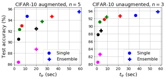
Figure 8: Performance-complexity tradeoff for single configs (circles) vs ensemble of configs (pluses) for $w_{c}=$ 0 (blue), 0.01 (red), 0.1 (green), 1 (black), 10 (pink). Results using ensemble of 5 for CIFAR-10 augmented, and 3 for CIFAR-10 unaugmented.

We experimented on CIFAR-10 unaugmented using $n=3$ and augmented using $n=5$. The impact on the performance-complexity tradeoff is shown in Fig. 8. Note how the plus markers – ensemble results – have slightly better performance at the cost of significantly increased complexity as compared to the circles – single results. However, we did not use ensembling in other experiments since the slight increases in accuracy do not usually justify the significant increases in $t_{\text{tr}}$.

Appendix: Changing hyperparameters of Bayesian Optimization

The BO process itself has several hyperparameters that can be customized by the user, or optimized using marginal likelihood or Markov chain Monte Carlo methods [29]. This section describes the default values we used. Expected improvement involves an exploration-exploitation tradeoff variable $\xi$. The recommended default is $\xi=0.01$ [7], however, we tried different values and empirically found $\xi=10^{-4}$ to work well. Secondly, $f$ is a noisy function since the computed values of network performance are noisy due to random initialization of weights and biases for each new state. Accordingly, and also considering numerical stability for the matrix inversions involved in BO, our algorithm incorporates a noise term $\sigma_{n}^{2}$. We calculated its value from the variance in $f$ values as $\sigma_{n}^{2}=10^{-4}$, which worked well compared to other values we tried.

Appendix: Adaptation to various platforms

While most deep NNs are run on GPUs, situations may arise where GPUs are not readily or freely available and it is desirable to run simpler experiments such as MLP training on CPUs. DnC can adapt its penalty metrics to any platform. For example, the FMNIST results shown in Fig. 4 were on CPU, while Table 3 shows results on GPU (to do a fair comparison with other frameworks). As a result, the $t_{\text{tr}}$ values are an order of magnitude faster, while the performance is the same as expected.

References

- [1] Private communication with authors regarding proxylessNAS (Mar 2020)
- [2] AWSLabs: AutoGluon: AutoML toolkit for deep learning. https://autogluon.mxnet.io/#
- [3] Baker, B., Gupta, O., Naik, N., Raskar, R.: Designing neural network architectures using reinforcement learning. In: Proc. ICLR (2017)
- [4] Baker, B., Gupta, O., Raskar, R., Naik, N.: Accelerating neural architecture search using performance prediction. In: Proc. ICLR (2017)
- [5] Baldi, P., Sadowski, P., Whiteson, D.: Searching for exotic particles in high-energy physics with deep learning. Nature Communications 5, 4308 (2014)
- [6] Bergstra, J., Yamins, D., Cox, D.D.: Making a science of model search: Hyperparameter optimization in hundreds of dimensions for vision architectures. In: Proc. ICML. p. I–115–I–123 (2013)
- [7] Brochu, E., Cora, V.M., de Freitas, N.: A tutorial on bayesian optimization of expensive cost functions, with application to active user modeling and hierarchical reinforcement learning. arXiv preprint arXiv:1012.2599 (2010)
- [8] Cai, H., Zhu, L., Han, S.: Hyperband: Bandit-based configuration evaluation for hyperparameter optimization. In: Proc. ICLR (2019)
- [9] Cai, H., Zhu, L., Han, S.: ProxylessNAS: Direct neural architecture search on target task and hardware. In: Proc. ICLR (2019)
- [10] Dey, S., Huang, K.W., Beerel, P.A., Chugg, K.M.: Pre-defined sparse neural networks with hardware acceleration. IEEE JETCAS 9(2), 332–345 (June 2019)
- [11] Dey, S., Shao, Y., Chugg, K., Beerel, P.: Accelerating training of deep neural networks via sparse edge processing. In: Proc. ICANN. pp. 273–280. Springer (2017)
- [12] He, Y., Lin, J., et al.: AMC: AutoML for model compression and acceleration on mobile devices. In: Proc. ECCV. pp. 784–800 (2018)
- [13] Huang, G., Sun, Y., et al.: Deep networks with stochastic depth. In: Proc. ECCV. pp. 646–661 (2016)
- [14] Hutter, F., Osborne, M.A.: A kernel for hierarchical parameter spaces. arXiv preprint arXiv:1310.5738 (2013)
- [15] Jin, H.: Comment on ‘not able to load best automodel after saving’ issue. https://github.com/keras-team/autokeras/issues/966#issuecomment-594590617
- [16] Jin, H., Song, Q., Hu, X.: Auto-keras: An efficient neural architecture search system. In: Proc. KDD. pp. 1946–1956 (2019)
- [17] Kandasamy, K., Neiswanger, W., et al.: Neural architecture search with bayesian optimisation and optimal transport. In: Proc. NeurIPS. pp. 2020––2029 (2018)
- [18] Krizhevsky, A., Sutskever, I., Hinton, G.E.: ImageNet classification with deep convolutional neural networks. In: Proc. NeurIPS. pp. 1097–1105 (2012)
- [19] Liu, C., Zoph, B., et al.: Progressive neural architecture search. In: Proc. ECCV. pp. 19–35 (2018)
- [20] Liu, H., Simonyan, K., Yang, Y.: DARTS: Differentiable architecture search. In: Proc. ICLR (2019)
- [21] Mayo, R.C., Kent, D., et al.: Reduction of false-positive markings on mammograms: a retrospective comparison study using an artificial intelligence-based CAD. J. Digital Imaging 32, 618–624 (2019)
- [22] Mendoza, H., Klein, A., et al.: Towards automatically-tuned deep neural networks. In: AutoML: Methods, Sytems, Challenges, chap. 7, pp. 141–156. Springer (2018)
- [23] Miikkulainen, R., Liang, J., et al.: Evolving deep neural networks. In: Artificial Intelligence in the Age of Neural Networks and Brain Computing, chap. 15, pp. 293 – 312. Academic Press (2019)
- [24] Page, D.: How to train your resnet. https://myrtle.ai/how-to-train-your-resnet/
- [25] Pham, H., Guan, M., et al.: Efficient neural architecture search via parameter sharing. In: Proc. ICML. pp. 4095–4104 (2018)
- [26] Real, E., Aggarwal, A., Huang, Y., Le, Q.V.: Regularized evolution for image classifier architecture search. In: Proc. AAAI. pp. 4780–4789 (2019)
- [27] Santana, E., Hotz, G.: Learning a driving simulator. arXiv preprint arXiv:1608.01230 (2016)
- [28] Snoek, J., Larochelle, H., Adams, R.P.: Practical bayesian optimization of machine learning algorithms. In: Proc. NeurIPS. p. 2951–2959 (2012)
- [29] Swersky, K., Duvenaud, D., et al.: Raiders of the lost architecture: Kernels for bayesian optimization in conditional parameter spaces. In: NeurIPS workshop on Bayesian Optimization in Theory and Practice (2013)
- [30] Tan, M., Le, Q.V.: Efficientnet: Rethinking model scaling for convolutional neural networks. arXiv preprint arXiv:1905.11946 (2019)
- [31] Thornton, C., Hutter, F., Hoos, H.H., Leyton-Brown, K.: Auto-WEKA: Combined selection and hyperparameter optimization of classification algorithms. In: Proc. KDD. pp. 847––855 (2013)
- [32] Xie, L., Yuille, A.: Genetic CNN. In: Proc. ICCV. pp. 1388–1397 (2017)
- [33] Zagoruyko, S., Komodakis, N.: Wide residual networks. In: Proc. BMVC. pp. 87.1–87.12 (2016)
- [34] Zoph, B., Vasudevan, V., Shlens, J., Le, Q.V.: Learning transferable architectures for scalable image recognition. In: Proc. CVPR. pp. 8697–8710 (2018)