Containment efficiency and control strategies for the Corona pandemic costs

Abstract

The rapid spread of the Coronavirus (COVID-19) confronts policy makers with the problem of measuring the effectiveness of containment strategies, balancing public health considerations with the economic costs of social distancing measures. We introduce a modified epidemic model that we name the controlled-SIR model, in which the disease reproduction rate evolves dynamically in response to political and societal reactions. An analytic solution is presented. The model reproduces official COVID-19 cases counts of a large number of regions and countries that surpassed the first peak of the outbreak. A single unbiased feedback parameter is extracted from field data and used to formulate an index that measures the efficiency of containment strategies (the CEI index). CEI values for a range of countries are given. For two variants of the controlled-SIR model, detailed estimates of the total medical and socio-economic costs are evaluated over the entire course of the epidemic. Costs comprise medical care cost, the economic cost of social distancing, as well as the economic value of lives saved. Under plausible parameters, strict measures fare better than a hands-off policy. Strategies based on current case numbers lead to substantially higher total costs than strategies based on the overall history of the epidemic.

Introduction

In March 2020 the World Health Organization (WHO) declared the Coronavirus (COVID-19) outbreak a pandemic [1]. In response to the growth of infections and in particular to the exponential increase in deaths [2], a large number of countries were put under lockdown, leading to an unprecedente recession [3] which could potentially have longer term costs [4]. In this situation it is paramount to provide scientists, the general public and policy makers with reliable estimates of both the efficiency of containment measures (e.g. social distancing and non-pharmaceutical health interventions), and the overall costs resulting from alternative strategies.

The societal and political response to a major outbreak like COVID-19 is highly dynamic, changing often rapidly with increasing case numbers. We propose to model the feedback of spontaneous societal and political reactions by a standard epidemic model that is modified in one key point: the reproduction rate of the virus is not constant, but evolves over time alongside with the disease in a way that leads to a ‘flattening of the curve’ [5]. The basis of our investigation is the SIR (Susceptible, Infected, Recovered) model, which describes the evolution of a contagious disease for which immunity is substantially longer than the time-scale of the outbreak [6]. A negative feedback-loop between the severity of the outbreak and the reproduction factor $g$ is then introduced. As a function of the control strength $\alpha_{X}$, which unites the effect of individual, social and political reactions to disease spreading, the difference between an uncontrolled epidemic ($\alpha_{X}=0$) and a strongly contained outbreak (large $\alpha_{X}$) is described, as illustrated in Fig. 1a. The model, which we name controlled-SIR model due to the presence of the control parameter $\alpha_{X}$, is validated using publicly available COVID-19 case counts from a large range of countries and regions. We provide evidence for data collapse when case counts of distinct outbreaks are rescaled with regard to their peak values. A comprehensive theoretical description based on an analytic solution of the controlled-SIR model is given. One finds substantial differences in the country-specific intrinsic reproduction factor and its doubling time. The controlled-SIR model allows in addition to formulate an unbiased benchmark for the effectiveness of containment measures, the containment efficiency index (CEI).

The controlled-SIR model is thoroughly embedded in epidemiology modeling. Early on, the study of the dynamics of measles epidemics [7] has shown that human behavior needs to be taken into account [8, 9]. In this regard, a range of extensions to the underlying SIR model have been proposed, such as including the effect of vaccination, contact-frequency reduction and quarantine [10], human mobility [11], self-isolation [12], the effects of social and geographic networks [13], the effects of awareness diffusion and epidemic propagation [14, 15], and the influence of explicit feedback loops [16]. For an in-depth description, epidemiology models need to cover a range of aspects [17], as the distinction between symptomatic and asymptomatic cases [18], which prevents in general the possibility of an explicit analytic handling. In the present work we pursue the alternative approach of retaining a minimal set of parameters, such that the resulting epidemiological model allows for an analytical description of the pandemic and its socio-economical aspects.

Political efforts to contain the pandemic, as social-distancing measures and non-pharmaceutical health interventions, are included in the controlled-SIR model as a dampening feedback mechanism. The controlled-SIR model is therefore suitable to estimate the overall economic and health-related costs associated with distinct containment strategies, in particular when accumulated over the entire course of an epidemic outbreak. This approach, which is followed here, extends classical studies of the economic aspects of controlling contagious diseases. A central question regards in this context the weighting of the economic costs of containment against the cost of treatment, and the loss of life [19, 20]. For the value of life, statistical approaches attribute suitably estimated monetary values to an avoided premature death [21, 22, 23]. The resulting framework has been applied to the Corona pandemic in several recent contributions in which the evolution of the epidemic has been taken in general as exogenous [24], relying on estimates for the infection [25] and case fatality rates [26, 27]. Further studies have discussed the relative effectiveness of control measures [25, 28, 29, 30, 31], and the possible future course of the disease [32, 33].

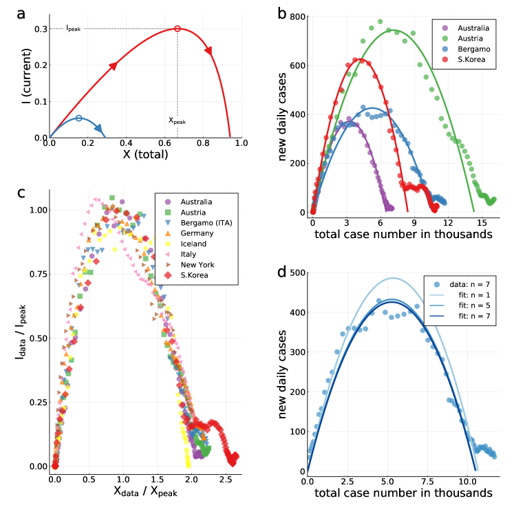
Figure 1: XI representation of COVID-19 outbreaks. a, Model illustration. The closed phase-space expression $I=I(X)$ of actual infected cases $I$ as a function of total infected cases $X$, as given by equation (3), is shown for two cases: $\alpha_{X}=0$ (no control, red line) and $\alpha_{X}=10$ (long-term control, blue line) for an intrinsic reproduction factor of $g_{0}=3$. The number of infections is maximal at $I_{\rm peak}$ (open circle), after starting at $X=I=0$, with the epidemic ending when the number of actual cases drops again to zero. At this point the number of infected reaches $X_{\rm tot}$. The peak $X_{\rm peak}=2/3$ of the uncontrolled case, $\alpha_{X}=0$, is sometimes called the ‘herd immunity’ point. The final fraction of infected is $X_{\rm tot}=0.94$. b, Model validation for a choice of four countries/regions. The model (lines) fits the seven-day centered averages of COVID-19 case counts well. For South Korea data till March 10 (2020) has been used for the XI-fit, at which point a transition from overall control to the tracking of individuals is observable. c, Data collapse for ten countries/regions. Rescaling with the peak values $X_{\rm peak}$ and $I_{\rm peak}$, obtained from the XI fit, maps COVID-19 case counts approximately onto a universal inverted parabola. d, Robustness test. The often strong daily fluctuations are smoothed by $n$-day centered averages. Shown are the Bergamo data (dots, $n=7$) and XI-fits to $n=1$ (no average), $n=5$ and $n=7$. Convergence of the XI-representation is observed.

Results

Controlled-SIR Model

In the following we introduce the model. At a given time $t$ we denote with $S=S(t)$ the fraction of susceptible (non-infected) individuals and $I=I(t)$ the fraction of the population that is currently ill (active cases). Infected individuals can either recover or die as a consequence of the infection, here we subsume both outcomes under $R=R(t)$, which denotes hence the fraction of recovered or deceased individuals. Normalization demands $S+I+R=1$ at all times. The continuous-time SIR model [34]

$$\tau\dot{S}=-gSI,\quad\quad\tau\dot{I}=(gS-1)I,\quad\quad\tau\dot{R}=I$$ (1)

describes an isolated epidemic outbreak characterized by a timescale $\tau$ and a dimensionless reproduction factor $g$. Social and political reactions reduce the reproduction factor below its intrinsic (medical disease-growth) value, $g_{0}$. We describe this functionality as

$$g=\frac{g_{0}}{1+\alpha_{X}X},\qquad\quad X=1-S\,,$$ (2)

where we generalized standard epidemiological approaches to nonlinear incidence rates [35, 36]. The reaction to the epidemic is taken to be triggered by the total fractional case count $X$ (i.e. the sum of active, recovered and deceased cases), with $\alpha_{X}$ encoding the reaction strength. In the Methods section we show how this functionality is validated by COVID-19 data, see also Fig. 2. In this view $\alpha_{X}$ sums up the effects of an extended number of social processes and political action taking. Further below we will examine in addition strategies for which the response is based on the fraction of actual active cases, $I$. We note that containment due to a reduction in the reservoir of susceptible $S$, is of minor importance, given that COVID-19 infection cases are generally small with respect to the overall population size.

The inverse functionality in equation (2) captures the law of diminishing returns, namely that it becomes progressively harder to reduce $g$ when increasing social distancing. In this view, small reductions of $g$ are comparatively easy, however a suppression by several orders of magnitude requires a near to total lockdown. We denote equation (1) together with (2) the controlled-SIR model. Key to our investigation is the observation that one can integrate the controlled-SIR model analytically, as shown in the Methods section, to obtain the phase-space relation

$$I=\frac{\alpha_{X}+g_{0}}{g_{0}}\,X+\frac{1+\alpha_{X}}{g_{0}}\,\log(1-X)\,.$$ (3)

This relation, which we denote the ‘XI representation’, is manifestly independent of the time scale $\tau$.

The medical peak load $I_{\rm peak}$ of actual infected cases is reached at a total fractional case count $X=X_{\rm peak}$, which is given by

$$gS=1,\qquad\quad X_{\rm peak}=\frac{g_{0}-1}{g_{0}+\alpha_{X}}\,,$$ (4)

For the case that $\alpha_{X}=0$ (no control), $X_{\rm peak}$ reduces to the well-known result $X_{\rm peak}=(g_{0}-1)/g_{0}$.

For finite $\alpha_{X}$, $I_{\rm peak}$ is obtained from equations (3) and (4),

$$I_{\rm peak}=\frac{g_{0}-1}{g_{0}}+\frac{1+\alpha_{X}}{g_{0}}\,\log\left(\frac{1+\alpha_{X}}{g_{0}+\alpha_{X}}\right)\,.$$ (5)

For $\alpha_{X}=0$, $I_{\rm peak}$ is sometimes called the ’herd immunity point’. The XI representation can be parameterized consequently either by $g_{0}$ and $\alpha_{X}$, as in equation (3), or indirectly by $X_{\rm peak}$ and $I_{\rm peak}$, which are measurable (modulo undercounting). In Fig. 1a an illustration of the XI-representation is given. For $g_{0}=3$ and $\alpha_{X}=0$ one has $X_{\rm peak}=2/3$ and $I_{\rm peak}\approx 0.3$. The total fraction of infected $X_{\rm tot}$ is 94%, which implies that only about 6% of the population remains unaffected. Containment policies, $\alpha_{X}>0$, reduce these values. Fig. 1a and equation (5) illustrate a sometimes encountered misconception regarding the meaning of the herd immunity point, which we have labeled simply $I_{\rm peak}$. The epidemic doesn’t stop at $I_{\rm peak}$ since infections continue beyond this point, albeit at a declining rate.

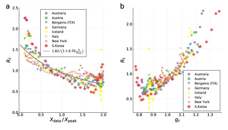
Figure 2: Validation of controlling feedback loop. The fraction of newly infected at time $t$ and at $t-4$ is used to estimate the time dependent reproduction factor $R_{t}=\overline{I}_{t}/\overline{I}_{t-4}$, when assuming a serial interval of four days (compare [37]). Note that a seven-day centred moving average $\overline{I}_{t}=\sum_{s=t-3}^{t+3}I_{s}$ is utilised. a, $R_{t}$ as a function of the relative cumulative number $X/X_{\rm peak}$ of cases. A fit to the same functional form as in equation (2) is given (grey line). b, correlation of $R_{t}$ and $g_{t}$. The estimated reproduction factor $R_{t}$ is compared to the effective reproduction factor $g_{t}$ as defined in equation (2). In a and b only data between $0.1\leq X/X_{\rm peak}\leq 2$ is shown, with the lower bound discarding the strong fluctuations in the early stages of the pandemic. The upper bound is used to define the termination of the first wave.

XI representation of COVID-19 outbreaks

In Fig. 1b,c we show for a representative choice of countries, regions and cities that COVID-19 outbreaks are described by the controlled-SIR model to an remarkable degree of accuracy. For the analysis presented in Fig. 1b,c we divided, as described in the Methods section, the official case counts by the nominal population size of the respective region or country. Seven-day centered averages are performed in addition. The country- and region-specific XI representations are then fitted by equation (3). The fact that the outbreaks are well described by the model, independently of the size of the country, region or city, evidences the applicability of the controlled-SIR model.

It has been widely discussed that official case counts are affected by a range of factors, which include the availability of testing facilities and the difficulty to estimate the relative fraction of unreported cases [38, 39]. For example, as of mid-March 2020, the degree of testing for COVID-19, as measured by the proportion of the entire population, varied by a factor of 20 between the United States (340 tests per million) and South Korea (6100 tests per million) [40]. The true incidence might be, according to some estimates [41] higher by up-to a factor of ten than the numbers reported in the official statistics as positive.

Case counts enter the XI representation in both the $x-$ and $y-$ axis. Scaling both $I$ and $X$ with a constant factor allows therefore to compensate for the undercounting problem. At the same time the control strength $\alpha_{X}$ needs to be rescaled, a procedure implicitly implemented for the fits shown in Fig. 1b,c. The XI framework is in this sense robust. Renormalization becomes however invalid if the undercounting of infection cases changes abruptly at a certain point during the epidemics, f.i. as a result of substantially increased testing. We will come back to this point further below. A fundamental change in the strategy followed by the government, e.g. from laissez faire to restrictive, would lead likewise to a change in $\alpha_{X}$, which is not captured in the current framework.

In the analysis presented in Fig. 1 daily case counts were taken as proxies for the number (relative fraction), of infected individuals $I=I(t)$. This assumption holds only up to a rescaling factor, which implies that the $g_{0}$ extracted for a given country or region is not the native, but an effective reproduction factor. To see this consider, e.g., the initial slope, $I\sim X(g_{0}-1)/g_{0}$, as given by equation (15). Rescaling daily case counts in order to obtain estimates for the number of infected individuals changes the slope and hence $g_{0}$. Given that the appropriate rescaling of daily case counts can only be estimated, and that we are interested here in a simple but accurate effective modeling of COVID-19 outbreaks, and not in the extraction of the native reproduction factor, we did not pursue this route.

In Table 1 we present for a number of countries and regions the obtained effective growth factors $g_{0}$ and the corresponding doubling times $\tau_{2}$, where $\tau_{2}=\log(2)/\log(g_{0})$ defines the number of time units $\tau$ needed to double case numbers. As expected, according to the description above, one finds that the values of $g_{0}$ are substantially lower than the consensus estimates 2-3 for the native reproduction number [42, 43, 44, 45, 46]. The observed doubling times $\tau_{2}$ are however retained when adapting the effective time scale $\tau$ accordingly.

For a robustness check we evaluated the parameters of the controlled-SIR model assuming that only a fraction $f$ of the nominal population of the country or region in question could be potentially infected, possibly due to the presence of social or geographical barriers to the disease spreading. Only marginal differences were found for $f=1/3$. The data presented in Table 1 suggest most countries followed in the first wave of the COVID-19 pandemic strict containment policies, as measured in terms of the CEI index. This insight is of particular relevance for the discussion of the costs incurring for the various containment strategies presented further below.

Data collapse for COVID-19

Given that the XI representation is determined solely by two quantities, $X_{\rm peak}$ and $I_{\rm peak}$, universal data collapse can be attained by plotting field data normalized with regard to the respective peak values, viz by plotting $I/I_{\rm peak}$ as a function of $X/X_{\rm peak}$. It is remarkable, to which degree the country- and region specific official case counts coincide in relative units, see Fig. 1c. It implies that the controlled-SIR model constitutes a faithful phase-space representation of epidemic spreading subject to socio-political containment efforts.

Table 1: COVID-19 containment efficiency index. For selected countries/ regions, key COVID-19 parameters, as extracted from the respective official case counts. Given is the dimensionless reproduction factor $g_{0}$, the doubling time $\tau_{2}=\log(2)/\log(g_{0})$, in units of $\tau$, and the containment efficiency index $\mbox{CEI}=\alpha_{X}/(g_{0}+\alpha_{X})$. Note that $g_{0}$ is not the native, but an effective reproduction factor.

location $g_{0}$ $\tau_{2}$ CEI Italy ITA 1.17 4.4 0.991 Iceland ISL 1.19 4.0 0.983 Bergamo ITA 1.20 3.8 0.972 Roma ITA 1.20 3.8 0.998 Germany DEU 1.21 3.6 0.995 United States USA 1.22 3.5 0.994 Spain ESP 1.23 3.3 0.990 Luxembourg LUX 1.28 2.8 0.988 Austria AUT 1.30 2.6 0.997 Israel ISR 1.30 2.6 0.997 Australia AUS 1.32 2.5 0.999 South Korea KOR 1.46 1.8 1.000

Asymmetry of up-/down time scales

For the controlled SIR model an explicit analytic expression for the $X-I$ phase space representation can be derived, as given by equation (3), but not for the complete timeline $X(t)$ and $I(t)$. Exploiting the fact that case counts are generally small with respect to the population for real-world epidemic outbreaks, the universal relation

$$\frac{\mbox{time down from the peak}}{\mbox{time up to the peak}}=2g_{0}-1$$ (6)

between the time the outbreak needs to retreat from the peak, and to reach it in first place, can however be found, as shown in the Methods section. Interestingly, the ratio of down-/ and up-times is independent of the control strength $\alpha_{X}$ (if and only if $X\ll 1$), which suggests that equation (6) is valid for epidemic outbreaks in general. For COVID-19, typical values of the effective $g_{0}$ are of the order of 1.2-1.3, as listed in Table 1, which implies that outbreaks take of the order of 40-60% longer to retreat than to ramp up.

Containment efficiency index

The control strength $\alpha_{X}$ enters the reproduction factor as $\alpha_{X}X$, see equation (2). Data collapse suggest that regional and country-wise data is comparable on a relative basis. From $\alpha_{X}X=(\alpha_{X}X_{\rm peak})(X/X_{\rm peak})$ it follows that $\alpha_{X}X_{\rm peak}=\alpha_{X}(g_{0}-1)/(g_{0}+\alpha_{X})$ is a quantity that measures the combined efficiency of socio-political efforts to contain an outbreak. Dividing by $g_{0}-1$ results in a normalized index, the ‘Containment Efficiency Index’ (CEI):

$$\mbox{CEI}=\frac{\alpha_{X}X_{\rm peak}}{g_{0}-1}=\frac{\alpha_{X}}{g_{0}+\alpha_{X}}\,,$$ (7)

with $\mbox{CEI}\in[0,1]$. The index is unbiased, being based solely on case count statistics, and not on additional socio-political quantifiers. Our estimates are given in Table 1. The values for the evaluated regions/ countries are consistently high, close to unity, the upper bound, indicating that the near-to-total lockdown policies implemented by most countries have been effective in containing the spread of COVID-19. A somewhat reduced CEI value is found for the particularly strongly affected Italian region of Bergamo. For South Korea the CEI is so high that its deviation from unity cannot be measured with confidence.

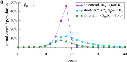
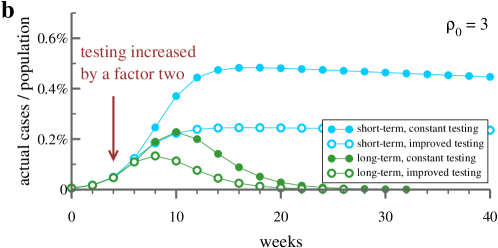
Figure 3: Control of epidemic peak. a, Shown is the timeline of actual infected cases during an epidemic outbreak with an intrinsic reproduction factor of $\rho_{0}=3.0$ defined in the discrete model, which is close to COVID-19 estimates [47]. The simulation is obtained by iterating equation (9), with one iteration corresponding to two weeks, taken as the average duration of the illness. Short-term control, when responding to the actual number of cases, see equation (8), is able to reduce the peak strain on the hospital system, but only by prolonging substantially the overall duration. Long-term control, which takes the entire history of the outbreak into account, is able to reduce both the peak and the duration of the epidemic. b, Increasing testing by a factor two (arrow), reduces the undercounting factor which increases, in turn, the effective response strength for both, the peak number of actual cases and the duration of the outbreak. Here $(\alpha_{X},\alpha_{I})=(400,0)\,/\,(0,400)$ has been used respectively for long- / short-term control.

Long-term vs. short-term control

So far, in equation (2) it was assumed that society and policy makers react to the total case count of infected $X$. This reaction pattern, which one may denote as ‘long-term control’, describes field data well. It is nevertheless of interest to examine an alternative, short-term control:

$$g=\left\{\begin{array}[]{lcl}g_{0}/(1+\alpha_{I}I)&&\mbox{(short-term)}\\[2.15277pt] g_{0}/(1+\alpha_{X}X)&&\mbox{(long-term)}\\ \end{array}\right.$$ (8)

For short-term control the relevant yardstick is given by the actual case number of infected $I$. In reality, people will react to officially reported case counts, which are affected by the undercounting problem. For the terms $\alpha_{I}I$ and and $\alpha_{X}X$ in equation (8) this corresponds to a renormalization of reaction parameters $\alpha_{I}$ and $\alpha_{X}$.

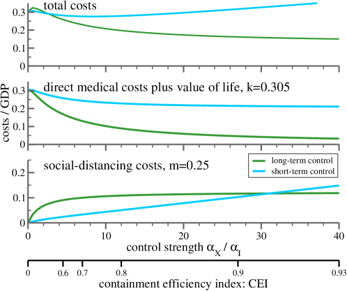
Figure 4: Cost of epidemic control strategies including value of life. Shown are the costs in terms of GDP_p.c., for long-term and short-term control, as defined by equation (8), both as a function of $\alpha_{X}$ and the CEI values (7), as indicated by the additional axis at the bottom. Given are the costs incurring from social distancing, equation (10) with $m=0.25$ (lower panel), the pure medical costs with value of life costs (middle panel), and the sum of social and medical costs (upper panel). It is assumed that the containment policy switches from mass control to individual tracking when the fraction of actual cases $I_{t}$ drops below a threshold of $I_{\rm min}=10^{-5}$. The starting $I_{0}=2\cdot 10^{-5}$.

Both control types, short- and long-term, can be employed either for the continuous-time SIR model, equation (1), or for the discrete-time variant,

$$I_{t+1}=\rho_{t}I_{t}(1-X_{t}),\quad\quad X_{t}=\sum_{k=0}^{\infty}I_{t-k}\,,$$ (9)

The time-dependent reproduction factor has been denoted here as $\rho_{t}$, in order to make clear that discrete times are used. Short- and long-term control is then equivalent to $\rho_{t}=\rho_{0}/(1+\alpha_{I}I)$ and $\rho_{t}=\rho_{0}/(1+\alpha_{X}X)$. One time step corresponds for the discrete-time SIR model to the mean infectious period.

The simulations of equation (9) presented in Fig. 3 illustrate the capability of short-term and long-term reaction policies to contain an epidemic. While both strategies are able to lower the peak of the outbreak with respect to the uncontrolled ($\alpha_{X}=\alpha_{I}=0$) case, the disease will become close to endemic when the reaction is based on the actual number of cases, $I_{t}$, and not on the overall history of the outbreak.

Also included in the lower panel of Fig. 3 is a protocol simulating an increase of testing by a factor of two. Here $(\alpha_{X},\alpha_{I})=(400,0)$ and $(\alpha_{X},\alpha_{I})=(0,400)$ have been used as the starting reaction strengths, respectively for long- and short-term control, which are increased by a factor of two when testing reduces the undercounting ratio by one half. One observes that long-term control is robust, in the sense that increased testing contributes proportionally to the containment of the outbreak. Strategies reacting to daily case number are in contrast likely to produce an endemic state.

The framework developed here, equations (1) and (2), describes mass control strategies, which are necessary when overly large case numbers do not allow to track individual infections. The framework is not applicable once infection rates are reduced to controllable levels by social distancing measures. The horizontal ’tail’ evident in the data from South Korea in Fig. 1b can be taken as evidence of such a shift from long-term mass control to the tracking of individual cases.

Costs of controlling the COVID-19 pandemic

As shown above, the controlled-SIR model allows for a faithful modeling of the entire course of an isolated outbreak. We apply it now to investigate how distinct policies and societal reaction patterns, as embedded in the parameter $\alpha_{X}$, influence the overall costs of the epidemic. This is an inter-temporal approach since the cost of restrictions today to public life (lockdowns, closure of schools, etc.) must be set against future gains in terms of lower infections (less intensive hospital care, fewer deaths). Four elements dominate the cost structure: (i) The working time lost due to an infection, (ii) the direct medical costs of infections, (iii) the value of life costs, and (iv) the cost related to ‘social distancing’. The first three are medical or health-related. All costs can be scaled in terms of GDP per capita (GDP_p.c.). This makes our analysis applicable not only to the US, but to most countries with similar GDP_p.c., e.g. most OECD countries.

Overall cost estimates

The cost estimates, which are given in detail in the Supplementary Information, can be performed disregarding discounting. With market interest rates close to zero and the comparatively short time period over which the epidemic plays out, a social discount rate between 3% and 5% would make little difference over the course of one year [48].

Total health costs $C^{\rm medical}$ incurring over the duration of the epidemic are proportional to the overall fraction $X_{\rm tot}=X_{t\to\infty}$ of infected, with a factor of proportionality $k$. We hence have $C^{\rm medical}=kX_{tot}$. We estimate $k\approx 0.305$ in terms of GDP_p.c. when all three contributions (working-time lost, direct medical cost, value of life) are taken into account, and $k\approx 0.14$ when value of life costs are omitted.

The economic costs induced by social-distancing measures, $C^{\rm social}$, depend in a non-linear way on the evolution of new cases (short-term control) or the percentage of the population infected (long-term control). To be specific, we posit that the reduction of economic activity is percentage-wise directly proportional to the relative reduction in the reproduction factor [49], viz to $(\rho_{0}-\rho_{t})/\rho_{0}$:

$$C^{\rm social}=\sum_{I_{t}>I_{\rm min}}\mbox{c}_{t}^{\rm s},\quad\quad\mbox{c}_{t}^{\rm s}=m\ \frac{\rho_{0}-\rho_{t}}{\rho_{0}}\,\frac{2}{52}\,,$$ (10)

where $2/52$ is the per year fraction of 2-week quarantine period. The epidemic is considered to be under control when the fraction of new infections $I_{t}$ falls below a minimal value $I_{\rm min}$. As detailed out in the Supplementary Information, a comprehensive analysis yields $m\approx 0.25$ in terms of GDP_p.c.. Note that the ansatz equation (10) holds only when mass control is operative, viz when large case numbers do not allow the tracking of individual infections.

Once $k$ and $m$ are known, one can compare the total costs incurring as the result of distinct policies by computing the sum of future costs for different values for $\alpha_{X}$ in equation (2). This is illustrated in Fig. 4 with the value of life costs included ($k=0.305$), and in Fig. 5, without value of life costs ($k=0.14$). Given are the total cumulative costs for the two strategies considered, long-term and short-term control, both as a function of the respective implementation strength, as expressed by the value of $\alpha_{X}$ and $\alpha_{I}$.

The middle panel of Fig. 4 shows that a society focused on short-term successes will incur substantially higher medical costs, because restrictions are relaxed soon after the peak. By contrast, if policy (and individual behavior) is influenced by the total number of all cases experienced so far, restrictions will not be relaxed prematurely and the medical costs will be lower for all values of $\alpha_{X}$. The bottom panel shows the social distancing costs as a fraction of GDP_p.c., which represent a more complicated trade-off between the severity of the restrictions and the time they need to be maintained. If neither policy, nor individuals react to the spread of the disease ($\alpha_{X}=0$) the epidemic will take its course and costs are solely medical. This changes as soon as society reacts, i.e. as $\alpha_{X}$ increases. Social distancing costs increase initially (i.e. for small values of $\alpha_{X}$), somewhat stronger for the long-term than for the short-term reaction framework. The situation reverses for higher values of $\alpha_{X}$ and $\alpha_{I}$ with $\alpha_{X},\alpha_{I}\approx 30$ being the turning point. From there on, the distancing cost from a long-term based reaction falls below that of the short-term strategy. The sum of the two costs is shown in the uppermost panel. For large values of $\alpha_{X}$, $\alpha_{I}$ short-term policies result in systematically higher costs.

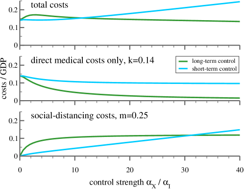
Figure 5: Cost of epidemic control without value of life. As in Fig. 4 (bottom panels are identical), but without the value of life costs. A long-term strategy with intermediate reaction strength is costlier than a hands-off policy.

Supplementary Figure 1 of the Supplementary Information shows that short-term control cannot explain observed COVID-19 outbreaks per se. Our estimates for the incurring costs suggest that economic cost considerations may have caused countries to follow predominantly long-term control strategies during the first wave of the COVID-19 outbreak.

Discussion

The total costs of competing containment strategies can be estimated if the feedback of socio-political measures can be modeled. For this one needs two ingredients: (i) a validated epidemiological model and (ii) a link between the impact of containment efforts, in terms of model parameters, to their economic costs. Regarding the first aspect, we studied the controlled-SIR model and showed that COVID-19 outbreaks follow in many cases the phase-space trajectory, the XI representation, predicted by the analytic solution. The same holds for the 2015 MERS outbreak in South Korea, as shown in Fig. 6b. We extracted for a number of countries and regions estimates for the intrinsic doubling times and found that they are not correlated to the severity of the outbreak. Regarding the second aspect, we proposed that the economic costs of social distancing are proportional to the achieved reduction in the infection rate [49]. Equation (10) establishes the required link between epidemiology, political actions and economic consequences. Health-related costs, which are related to official case counts, are in contrast comparatively easier to estimate. We have not considered formally the optimal control problem, which would consist of minimising the sum of total costs if the control strength could be chosen freely for every period. Instead, we have been interested here in comparing distinct containment strategies under which society and governments react in a predictable pattern to the spread of the disease.

A non-trivial outcome of our study is that strong suppression strategies lead to lower total costs than taking no action, when containment efforts are not relaxed with falling infection rates. A short-term control approach of softening containment with falling numbers of new cases is likely to lead to a prolonged endemic period. With regard to the ‘exit strategy’ discussion, these findings imply that social distancing provisions need to be replaced by measures with comparative containment power. A prime candidate is in this regard to ramp up testing capabilities to historically unprecedented levels, several orders of magnitude above pre-Corona levels. The epidemic can be contained when most new cases are tracked, as implicitly expressed by the factor $\alpha_{X}$. This strategy can be implemented once infection rates are reduced to controllable levels by social distancing measures. Containment would benefit if the social or physical separation of the ‘endangered’ part of the population from the ‘not endangered’ would be organized in addition on a country-wide level, as suggested by community-epidemiology. With this set of actions the vaccine-free period can be bridged.

As a last note, there is a sometimes voiced misconception regarding the meaning of the herd immunity point, which occurs for an infection factor of three when 66% of the population is infected. Beyond the herd immunity point, the infected-case counts remain elevated for a considerable time. The outbreak stops completely only once 94% of the population has been infected, as illustrated in Fig. 1a.

Methods

Validation of the model from COVID-19 data

In Fig. 2 we show how the model given in equation (2) is validated by COVID-19 data. Fig. 2a displays the collected data of infected population during the first wave of the COVID-19 pandemic in a range of representative countries and regions. Plotted is the time-dependent reproduction factor R_t as a function of the relative cumulative case count $X/X_{\rm peak}$. We followed standard procedures [37] and defined $R_{t}$ as the fraction of newly infected individuals at time $t$ with respect to the infected individuals at time $t-4$ days, $R_{t}=\overline{I}_{t}/\overline{I}_{t-4}$, where seven-day centered moving averages $\overline{I}_{t}=\sum_{s=t-3}^{t+3}I_{s}$ are considered. Also shown is a fit to the data using the functional form predicted by our model, equation (2). The quantitative comparison between field data and modeling validates the controlled-SIR model. For a set of representative countries and regions it is shown in Fig. 2b that there is a direct correlation between the measured reproduction factor $R_{t}$ and the effective reproduction factor $g_{t}$, as defined by equation (2).

Data collection and handling

Data has been accessed as of May 18 (2020) via the public COVID-19 Github repository of the Johns Hopkins Center of Systems Science and Engineering [50]. Preprocessing was kept minimal, comprising only a basic smoothing with sliding averages. If not stated otherwise, a seven time centered average (three days before/after, plus current day) has been used. Robustness checks with one, three and five day sliding averages were performed, as shown in Fig. 1d. Fractional case counts are obtained by dividing the raw number by the respective population size. For the case of South Korea, the XI-analysis was performed using the initial outbreak, up to March 10 (2020). China has been ommitted in view of the change in case count methodolgy mid February 2020.

The variable $I$ represents in the SIR model the fraction of the population that is infectious, which for this model coincides with the infected population. For the COVID-19 data, we used instead an XI-representation for which the number of new daily cases is plotted against the total case count. This procedure is admissible as long as the relative duration of the infectious period does not change.

Fitting procedure

We compared the theoretical result for the controlled SIR model, $I(X)\equiv I^{\rm(theory)}(X)$, see equation (3), to the reported data $I_{t}^{\rm(data)}$, where $t$ runs over all days. The field data $X_{t}^{\rm(data)}$ for the total case number is crowded at low levels of $X$ and $I$ in the XI representation. A fitting procedure that takes the range $X\in[0,X_{\rm tot}]$ uniformly into account is attained when minimizing the weighted loss function

$$U=\sum_{t}u_{t}\left(I_{t}^{\rm(data)}-I^{\rm(theory)}(X_{t}^{\rm(data)})\right)^{2}\,.$$ (11)

For the weight we used $u_{t}=X_{t}^{\rm(data)}-X_{t-1}^{\rm(data)}=I_{t}^{\rm(data)}$, which satisfies the sum-rule $\sum_{t}u_{t}=X_{\rm tot}$, where $X_{\rm tot}$ is the total (maximal) case count. With equation (11) it becomes irrelevant where the timeline of field data is truncated, both at the start or at the end. Adding a large number of null measurements after the epidemic stopped would not alter the result. Numerically the minimum of $U$ as a function of $g_{0}$ and $\alpha_{X}$ is evaluated.

Modeling field data as uncontrolled outbreaks

It is of interest to examine to which degree official case statistics could be modeled using an uncontrolled model, $\alpha_{X}=0$. For this purpose it is necessary to assume that the epidemics stops on its own, which implies that one needs to normalize the official case counts not with respect to the actual population, but with respect to a fictitious population size $N$. In this view the outbreak starts and ends in a socially or geographically restricted community. The results obtained when optimizing $N$ are included in Fig. 6a. At first sight, the $\alpha_{X}=0$ curve tracks the field data. Note however the very small effective population sizes, which are found to be 478000 for the case of Germany. Alternatively one may adjust $g_{0}$ by hand during the course of an epidemic, as it is often done when modeling field data.

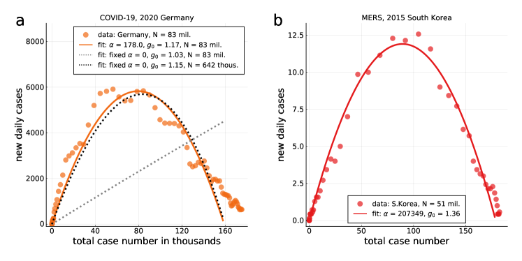
Figure 6: Case count modelling. a, Modeling case counts as uncontrolled outbreaks. Case counts, here for Germany (seven-day centered averages, dots), can be modeled using either the full XI representation (full line), as given by equation (3), or with the standard uncontrolled SIR model ($\alpha_{X}=0$, dashed lines). Using the nominal population size for Germany, 83 Million, leads to an utterly unrealistic $\alpha_{X}=0$ curve (dashed, grey). The best $\alpha_{X}=0$ fit is obtained when a fictitious population size of 478 Thousand is assumed (dashed, black). An epidemic abates on its own only when the population size is of the order of the total case count divided by $X_{\rm tot}$. b, XI representation of the 2015 MERS outbreak in South Korea, covering a total of 186 cases. A $n=7$ centered average has been used, in view of the small case numbers.

Analytic solution of the controlled-SIR model

Starting with the expression for the long-term control, equation (2), one can integrate the controlled-SIR model equation (1) to obtain a functional relation between $S$ and $I$. Integrating $\dot{I}/\dot{S}$, viz

$$dI=-dS+\frac{1}{g(S)S}\,dS=-dS+\frac{1}{g_{0}}\,\frac{1+\alpha_{X}(1-S)}{S}\,dS\,,$$

yields

$$I=-\left(\frac{\alpha_{X}}{g_{0}}+1\right)S+\frac{1+\alpha_{X}}{g_{0}}\,\log(S)+c\,,$$ (12)

where the integration constant $c$ is given by the condition $I(S\!=\!1)=0$. Substituting $S=1-X$ one obtains consequently the XI-representation equation (3). The analogous result for $\alpha_{X}=0$ has been derived earlier [51]. The number of actual cases, $I$, vanishes both when $X=0$, the starting point of the outbreak, and when the epidemic stops. The overall number of cases, $X_{\rm tot}$, is obtained consequently by the non-trivial root $X_{\rm tot}$ of equation (3), as illustrated in Fig. 1a. As a side remark, we mention that the XI representation allows us to reduce equation (1) to

$$\tau\dot{S}=-\frac{gS}{g_{0}}\Big{[}(\alpha_{X}+g_{0})(1-S)+(1+\alpha_{X})\log(S)\Big{]}\,,$$ (13)

which is one dimensional. Integrating equation (13) with $g=g(S)$ yields $S=S(t)$, from which $I(t)$ follows via $\tau\dot{I}=\big{(}gS-1\big{)}I$ and $R(t)$ from the normalization condition $S+I+R=1$.

Large control limit of the XI representation

Expanding equation (3) in $X$, which becomes small when $\alpha_{X}\gg 1$, one obtains

$$I=\frac{1+\alpha_{X}}{2g_{0}}X\left[2\,\frac{g_{0}-1}{1+\alpha_{X}}-X\right]+O(X^{3})\,,$$ (14)

which makes clear that the phase-space trajectory becomes an inverted parabola when infection fractions are small. As a consequence one finds

$$I\approx\frac{g_{0}-1}{g_{0}}\,X+O(X^{2})\,,$$ (15)

which shows that the slope $dI/dX=(g_{0}-1)/g_{0}$ at $X\to 0$ is independent of $\alpha_{X}$ and of the normalization procedure used for $I$ and $X$. The first result was to be expected, as $\alpha_{X}$ incorporates the reaction to the outbreak, which implies that $\alpha_{X}$ contributes only to higher order. The dimensionless natural growth factor $g_{0}$ is hence uniquely determined, modulo the noise inherent in field data, by measuring the slope of the daily case numbers with respect to the cumulative case count.

From equation (14) one obtains

$$X_{\rm tot}\big{|}_{\alpha_{X}\gg 1}\approx 2\,\frac{g_{0}-1}{\alpha_{X}}\,$$ (16)

for the total number of infected $X_{\rm tot}$ in the large-control limit. In analogy one finds

$$I_{\rm peak}\big{|}_{\alpha_{X}\gg 1}\approx\frac{(g_{0}-1)^{2}}{g_{0}\alpha_{X}},\quad\quad X_{\rm tot}\approx\frac{2g_{0}}{g_{0}-1}\,I_{\rm peak}$$ (17)

from equation (3), and in comparison with equation (16).

Time scale asymmetry

From the one-dimensional representation (13) of the controlled SIR model one can estimates two characteristic time scales. For this purpose one considers an initial relative infection status $f_{X}X_{\rm tot}$, with $f_{X}>0$ and $f_{X}\ll 1$.

• run-up: $T_{\rm up}$, defined as the time needed to reach the peak when starting from $X_{\rm start}=f_{X}X_{\rm tot}$.

• run-down: $T_{\rm down}$, defined as the time needed to reach $X_{\rm end}=(1-f_{X})X_{\rm tot}$, down from the peak.

In general one needs to integrate equation (13) numerically. Given that real-world fractional case counts $X$ are small, $X<X_{\rm tot}\ll 1$, one can simplify (13), as for (14), obtaining

$$t-t_{0}=\frac{\tau}{g_{0}-1}\log\left(\frac{X}{(X_{\rm tot}-X)^{2g_{0}-1}}\right)\,.$$ (18)

It follows directly that $T_{\rm down}/T_{\rm up}=2g_{0}-1$, as stated in equation (6). For a pathogen to spread its dimensional growth factor $g_{0}$ needs to be larger than unity, compare Table 1. Going down takes hence substantially longer than ramping up.

Data availability

The COVID-19 data examined is publicly accessible via the COVID-19 Github repository of the John Hopkins Center of Systems Science and Engineering
https://github.com/CSSEGISandData/COVID-19.
Data for the 2015 MERS outbreak in South Korea is publicly available from the archive of the World Health organization (WHO),
https://www.who.int/csr/disease/coronavirus _infections/archive-cases/en/.

Author contributions

Modeling and theory by C.G. and R.V, data analysis by L.S., medical aspects by K.V, economical and political topics by D.G.

Competing interests

The authors declare no competing interests.

Additional information

Correspondence and requests for materials should be addressed to C.G.

SUPPLEMENTARY INFORMATION

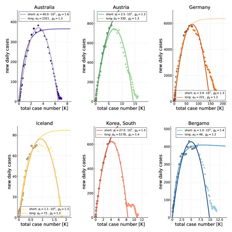
Supplementary Figure 1: $|$ Short- vs.- long-term containment. Fits to COVID-19 data for short-term control, $(\alpha_{I},\alpha_{X})=(\alpha_{I},0)$ and, for comparison, for long-term control, $(\alpha_{I},\alpha_{X})=(0,\alpha_{X})$. The parameter value are given in the respective legends. The intial slope, which reflect the initial phase of exponential growth, has been taken as a reference.

Societal reaction to the spread of the disease

The two strategies investigated here, short-term and long-term, correspond to reaction patterns that are observed for the COVID-19 outbreak [52, 53]. In Supplementary Figure 1 we present some examples. For both cases, the societal reaction described by the parameter $\alpha_{X}$ and $\alpha_{I}$ can be thought as a sum of two contributions

$$\alpha_{X}=\alpha_{s}+\alpha_{g},$$ (19)

where $\alpha_{s}$ quantifies the spontaneous reaction by the population and $\alpha_{g}$ encodes government interventions. Analogously, such a sum of two contributions can be made for $\alpha_{I}$.

The first contribution, $\alpha_{s}$, takes into account societal behavioral changes happening when a substantial fraction of the population spontaneously adopts social distancing (avoiding hand-shakes, restaurants, cinemas, etc.), f.i. in response to media reports about the severity of the outbreak. Voluntary social distancing can lead to substantially reduced restaurants and cinemas attendances even before governments impose mandatory school closures, curfews and other drastic measures.[54] An important aspect of the spread of COVID-19 is the distinct reactions of societies in different countries. In Asia the wearing of masks becomes a convention, which is likely to correspond to a higher $\alpha_{s}$, while such a measure tends to be resisted by a majority of European populations.[55]

The second contribution to the control factor, $\alpha_{g}$, captures the role of government interventions. Measures ranging from forbidding large events, to school closures and, finally, to lockdowns, become politically possible when the number of individuals infected increases and surpasses critical levels.

The aim of our investigation is not to evaluate the effectiveness of specific measures, which has been done elsewhere [28, 25], but to assess the dynamical effect of the societal reaction encoded in the feedback parameter $\alpha_{X}$, on the overall evolution of the epidemic. As most social distancing measures are costly, both for the economy and overall well-being[56], it is reasonable to assume that their strictness is increased only when necessary, viz in relation to the severity of the outbreak. The latter can be measured either by the number of current cases, $I_{t}$, or by the cumulative case count $X_{t}$.

The inverted U shape of the total cost of the virus as a function of $\alpha_{X}$ has one important corollary: the ’laissez faire’ equilibrium is not the optimum for society. If the government abstains from action leaving it to societal reaction to dampen the peak, the spread of the disease would be limited only by $\alpha_{s}$, which might bring society close to the hump of the total cost curve. Strong government action, i.e. a high value of $\alpha_{g}$ could then push the path to the other side of the hump resulting in lower costs. In other words, relying only on individual reaction which aims at lowering the risk to oneself, would be sub-optimal. This is of course a general result for all contagious diseases [20, 19] but we confirm it accounting explicitly for the cost of the measures needed to protect public health.

Detailed costs of controlling the COVID-19 pandemic

In what follows we present a detailed estimation of the costs of controlling the COVID-19 pandemic given in GDP per capita (GDP_p.c.) to ensure comparability across countries.

Four elements dominate the cost structure: (i) The working time lost due to an infection, (ii) the direct medical costs of infections, (iii) the value of life costs, and (iv) the cost related to ‘social distancing’. The first three are medical or health-related.

Health costs, loss of working time

A first direct impact of a wave of infections is that a fraction of the population cannot work. Based on the Diamond Princess data [57], where the entire population was tested, we estimate that only half of the infected develop symptoms that require them to stay home for a one- to two-week period and an additional two-week period until they are no longer contagious. About 20% of the infected (or 40% of those with symptoms) develop stronger symptoms requiring one additional period of absence from work [27]. To be conservative, we assume that there are no severe cases or deaths among the working age. This results in a reduction in the work force per year (52 weeks) of around $(0.3\times 2+0.2\times 3)\times(2/52)=2.4/52=0.05$, for every 1% of the population infected.

Medical costs, treatment, hospitalization

Hospitalization rates and costs of hospital treatment for COVID-19 vary enormously across across countries. But it is estimated that about 20% [58] of the infected individuals require some sort of hospitalization. A recent large scale survey of the literature[59] shows that about one fourth of them (around 5% of the infected) need intensive care and roughly on sixth dying. We adopt a more conservative fatality rate among the hospitalized of 1% [57].

As a comparison, we note that an average influenza season leads to a hospitalization of about 0.12% of the US population [60]; and one fourth of them require intensive care, with one twentieth (0.13% of all infected) dying [57]. Averaged over the 2010-17, of the order of 35 thousand influenza-related deaths per year have been registered in the US, one tenth of the over 300 thousand COVID-19 related fatalities registered in 2020.

Costs: Intensive care with ventilation is the most costly form of life saving in hospital care[59]. In the US, the cost of two weeks of an intensive care unit is equivalent to about 1 year (100%) of GDP_p.c. [61]. For Covid-19 patients in the US, it has been reported that average hospitalisation costs per case amount to over 70 thousand USD, or 115% of (annual) GDP per capita [62].

In Germany, which might be typical of the rest of Europe, the cost of two weeks of intensive care appears to be lower, around 20,000 Euro, or roughly 60% of GDP_p.c. [63]. We use the German parameters for a conservative estimate of medical costs. The cost of general hospitalization for two weeks is assumed to be 12,000 Euro, and equivalent to about 30% of GDP_p.c.. With two weeks of general hospitalization and two weeks of intensive care for severe cases, this results in a medical cost of $(0.05\times 0.6+0.05\times 0.3+0.15\times 0.3=0.09)$, that is of 9% GDP_p.c..

Value of lives lost

Third, the cost of premature death through the disease represents the most difficult element to evaluate in financial terms. We will show below that our central results remain valid even without assigning a monetary value to lives lost, but since major contributions [24] are based on an evaluation of the economic value of lives lost, we show how this point can be incorporated into our framework. There are two ways to attribute a monetary value on a life saved or lost. The first, mentioned in the main text, is based on the concept of a Value of Statistical Life (VSL), which is commonly used in the impact assessment of public policy that aims at lowering the probability of a premature death [64]. A typical application scenario for VSL is the case when the probability of death is very low (e.g. car accidents), but could be lowered even more (seat belts). For COVID-19, a high-death epidemic, we prefer a medical-based approach, which allows us to produce conservative estimates. VSL arrives in contrast often at much higher values, up to millions of Euro or Dollars [65]. Putting a monetary value on lives saved is unavoidable in medical practice that is confronted with the problem of selecting the procedures to be used to prolong life - a situation that arises for many patients infected by the Coronavirus under intensive care.

The literature dealing with the cost of medical procedures finds a central range of between 100,000 and 300,000 Dollars per year of life lost [66, 67]. Given the current US GDP_p.c., these values translate into a range of 1.5 to 4 years of GDP_p.c.. Cutler and Richardson [68] argue for a value equivalent to three times GDP_p.c.. We use the lower bound of this range (i.e. 1.5 times GDP_p.c.) for most of our simulations, which might thus under-estimated the value of lives saved through social distancing restrictions.

What remains to be determined is the number of years lost when a Corona patient dies.

On the cruise ship Diamond Princess [57, 26] which served almost as a laboratory, the average age at death was 76 years. Cruise passengers tend to have fewer acute health conditions than the general population, thus rendering the co-morbidity argument less prominent. The remaining life expectancy (weighted by the difference incidence by sex) would thus be 11 years. This implies that the economic value of the premature deaths should be equal to about 11 times the loss for one year of life saved (potentially higher for most European countries which tend to have a higher life expectancy).

For each 1% of the population the value of lives lost would thus be equal to $0.01\times 11\times$ the nominal value of one year of life.

The value of life can be measured in terms of multiples of GDP_p.c., which allows to write the sum of the three types of health or medical costs (loss of working time, hospitalization and value of lives lost) as a linear function of the percentage of the population infected:

$$c_{t}^{\rm med}=kI_{t}$$

with a proportionality factor $k$ being equal to the sum of the three contributions. Scaling $k$ with the GDP_p.c. allows for an application and comparison across countries. Using the lower bound of the central range yields then the following calibration of the medical costs:

$$(0.05+0.09+0.01\times 1.5\times 11)\times\mbox{GDP}_{\rm p.c.} =$$

$$0.305\times\mbox{GDP}_{\rm p.c.}$$ (20)

The upper bound for the value of $k$ would be substantially higher: $(0.05+0.09+0.01\times 4\times 11)\times\mbox{GDP}_{\rm p.c.}=0.58\times\mbox{GDP}_{\rm p.c.}$. For the numerical calculations we will use the conservative estimate $k=0.305$ in terms of GDP_p.c..

If we only consider the direct medical costs consisting of loss of working time and hospitalization, without including the value of lives lost, the proportionality factor in equation (20) reduces to $k=0.14$ in terms of GDP_p.c..

Medical costs over the lifetime of the epidemic

The cost estimates discussed so far, $c_{t}^{\rm med}$, refer to the per-period cost of the currently infected. For the total cost over the entire endemic we need to calculate the discounted sum of all $c_{t}^{\rm med}$ over time. Given that a period corresponds to about two weeks, we neglect discounting, which would make little difference even if one uses a social discount rate of 5% instead of using market rates (which may be negative). The total medical costs over the course of the endemic can be written as the simple sum of the cost per unit of time:

$$C^{\rm medical}=\sum_{I_{t}>I_{\rm min}}c_{t}^{\rm med}=kX_{tot}\,.$$ (21)

The epidemic is considered to have stopped when the fraction of new infections $I_{t}$ falls below a minimal value, $I_{\rm min}$.

Using the conservative estimate (low value of life) $k$ = 0.305 it is straightforward to evaluate the total cost of a policy of not reacting at all to the spread of the disease, which would lead in the end to $X_{\rm tot}=0.94$. A hands-off policy would therefore lead to medical costs of over 28% of GDP.

In absolute terms the cost of a policy of doing nothing would amount to 1000 billion Euro for a country like Germany. For the US the sum would be closer to 5 Trillion of Dollars (25% of a GDP of 20 Trillion of Dollars). As it would not be possible to ramp up hospital capacity in the short time given the rapid spread of the disease, the cost would be in reality substantially higher, together with the death toll [24, 25]. We abstract from the question of medical capacity (limited number of hospital beds) because we assume that society would react anyway as the virus spreads, thus limiting the peak, and, second, we are interested in the longer term implications of different strategies and not just in their impact on the short-term peak.

We note that even concentrating only on the direct medical cost and working time lost ($k$=0.14) a policy of letting the epidemic run its course through the entire population would lead to losses of working time and hospital treatment of over 13% of GDP (94% of 14%). By comparison, total health expenditure in most European countries amounts in normal times to about 11% of GDP [69]. Even apart from ethical considerations, to avoid or not potentially hundreds of thousands of premature deaths, there exists thus an economic incentive to slow the spread of the COVID-19 virus.

Given the somewhat contentious nature of the value of lives lost, we present in the middle panel of Fig. 4 of the main text the medical cost estimates (as a proportion of GDP) without including the value of life costs (results with including the value of life costs are shown in the main text). As shown in the figure, increasing $\alpha_{X}$ leads to a lower medical cost because the percentage of the population infected will be lower. The difference between short-term and long-term control increases for higher values of $\alpha_{X}$. At these $\alpha_{X}$ values the medical cost over the entire endemic would be lower because the overall fraction of infected population is lower. For a strongly reactive society and policy i.e. for $\alpha_{X}\gg 1$ (and the case of long-term control), an explicit solution for the total health cost is given by,

$$C^{\rm medical}=kX_{\rm tot}\big{|}_{\alpha_{X}\gg 1}\approx 2k\,\frac{g_{0}-1}{\alpha_{X}}\,$$ (22)

which implies that the total health or medical costs are inversely proportional to the strength of the policy reaction parameter. Draconian measures from the start, i.e. with $\alpha_{X}$ going towards infinity, reduce the medical costs to close to zero - irrespective of whether one adds the value of lives lost. This can be seen in Fig. 3 and Fig. 4 of the main text, where the medical cost (over the entire epidemic) starts for $\alpha_{X}=0$ at values close to $k$ because without any societal reaction 94% of the population would get infected and with increasing $\alpha_{X}$ the medical costs decline monotonously.

Social distancing costs

The economic costs of imposing social distancing on a wider population are at the core of policy discussions and drive financial markets. As mentioned above, social distancing can take many forms; ranging from abstaining from travel or restaurant meals to government interventions enforcing lockdowns, quarantine, closure of schools, etc. This cost is more difficult to estimate. However, a rough estimate is possible if one takes into account that most economic activity involves some social interactions. Limiting social interaction thus necessarily reduces economic activity. This suggests that the economic cost of the social distancing described in equation (2) of the main text should increase with the reduction in the transmission rate described by $g$.

Without any social distancing, $\alpha_{X}=0$, the economy would not be affected by the spread of the virus. Stopping all economic social interactions would bring the economy to a halt, but the reproduction rate of the virus would also go close to zero (Eichenbaum et al. [70] make a similar assumption). We thus posit that the (per-time unit) social-distancing economic cost ${c}_{t}^{\rm s}$ is proportional to the reduction in the transmission rate. The total economic costs $C^{\rm social}$ can be written as the sum of ${c}_{t}^{\rm s}$:

$$C^{\rm social}=\sum_{I_{t}>I_{\rm min}}\mbox{c}_{t}^{\rm s},\quad\quad\mbox{c}_{t}^{\rm s}=m\left[1-\frac{\rho_{t}}{\rho_{0}}\right]\frac{2}{52}$$ (23)

considering here the notation of the discrete-time controlled SIR model (equation (8)). The key question is the factor of proportionality, $m$, which links the severity of social distancing to the reduction in economic activity. Popular attention has focused on services linked directly to social contact. There exist indeed selected sectors which will completely shut down under a lockdown. However, these sectors (tourism, non-food retail, etc.) account for a limited share of the economy (less than 10% for most countries). Expenditure for food is actually little affected since even under the most severe lockdown, grocery shopping is still allowed and families must consume more food at home as they cannot go out to restaurants.

The manufacturing sector is less affected by social distancing than the service sector because in modern factories workers are scattered over a large factory floor, making it relatively easy to maintain production while maintaining the appropriate distance between workers. Moreover, some sectors, e.g. finance, can work online with only a limited effect on productivity. The widespread impression that the entire economy stops under a lockdown is thus not correct. The drastic measures adopted in China illustrate this proposition: when all non-essential social interactions were forbidden, industrial production and retail sales fell by ’only’ 20-25% [71] while the reproduction factor went from 3 to 0.3, a fall by a factor of ten. Using this experience we calibrate the parameter $m$ at 0.25. The projections of the International Monetary Fund, a loss of output of about 8% for severe lockdowns lasting one quarter [3], [72] confirm this order of magnitude.

A reduction in the reproduction factor $\rho_{t}$ to one tenth its normal epidemiological value of $\rho_{0}$ would thus lead to a loss of GDP of 25% for the time period during which the restriction or social distancing measures are in place. This would imply that an abrupt shutdown of the economy to 25% of its capacity for 12 weeks, or 6 incubation periods would cost about 0.25$\times$(12/52), or about 6% of annual GDP. A reduction of GDP by 6% represents a recession even deeper than the one which followed the financial crisis of 2009. This is compatible with current forecasts of zero GDP growth in China in 2020 (relative to a baseline of 5-6% before the crisis). But even such a large cost in terms of output foregone would be below the medical cost arising from herd immunity[73]. Even apart from ethical considerations, it would thus appear to make sense to accept a temporary shut down of parts of the economy to avoid the huge medical costs.

A first result is thus that if one compares two extremes: letting contagion run its course (herd immunity) or draconian measures, the social costs are lower in the second case. Small changes to the key parameters, $k$ and $m$, might change the exact values of the costs in terms of overall magnitude, but the ranking appears robust.

We do not consider separately the fiscal cost, i.e. the cost for the government to save millions of enterprises from bankruptcy and ensure that workers have a replacement income when they get laid off. This cost to governments is a transfer within the country from one part of society (tax payers) to those who suffer most under the economic crisis.

A key issue in the discussion on the economic cost of social distancing is the question about how long these measures need to be maintained. It is sometimes argued that the cost of a policy of social distancing would be unacceptably high because the measures could not be relaxed until the virus had been totally eradicated. However, this pessimism is not warranted by the success of a strategy of ‘testing and tracing’ implemented in some countries (mainly those which had experienced SARS). Such a strategy is, of course, only possible if the starting number of infections is low enough to allow for individual tracing.

We thus make the assumption that when the number of active cases falls below a certain threshold, the costly measures of general social distance containment are no longer needed and can be substituted by pro-active repeated testing coupled to quick follow-up of the remaining few cases which are quarantined and whose contacts are quickly traced. In this case the resulting economic cost is assumed to fall away. The experience of Taiwan[74], Korea[75] and Japan suggests that when the infected are less than one per 100,000, general social distancing is no longer required (assuming mass testing has been adopted in the meantime so that the infections can be accurately measured).

Parameter updating
The estimates on which our results are based will have to be updated when actualized COVID-19 data is available in the future. The WHO-China Joint Mission Report suggests a $\rho_{0}$ ($g_{0}$ in the continuous-time representation) per infected of $2-2.5$ [76] (in units of the disease duration), while we use the figures from Liu et al. [47], who predict a reproduction factor of around three. The numbers for the forecast of health costs are derived in part from the Diamond Princess data [57], for which the population was comparatively healthy. The statistics for symptoms requiring the absence from work may therefore in reality be somewhat higher.

The hospitalization and mortality rate are estimated with a substantial uncertainty, due to the high numbers of unregistered and untested infections. Early studies based on official data from China [77, 78] estimated that the number of actual infections may be between 10 to 20 times higher than the number of detected infections. However, serological test in e.g. Austria suggest only a factor of 3 [79]. The continuing screening of blood samples via the US, Nationwide Commercial Laboratory Seroprevalence Survey, showed in September 2020 an average undercounting factor of 2.6, as opposed to our assumption of 2. Leaving possibly lower, but still substantial true hospitalization and mortality rates for COVID-19.

A strong age gradient has been observed for the case fatality rate of COVID-19 by age[80], which could be logistic[81], and there are large variations across countries[82]. Moreover, one has to take into account that while case fatality rates are much lower for the younger, they are represent a larger share of the population and their life expectancy is also higher (e.g. over 20 years for the 60 years old). These two factors tend to give more weight to the younger age brackets, leading to resulting parameter estimates similar to ours [83].

One of our main goals has been the introduction of a generic framework, which can be updated by further advances in the accuracy of estimates while still presenting specific results with the data available at this time.

Relation to further studies
A range of determining factors have been examined for the ongoing COVID-19 epidemic, in particular the effect of quarantine [84] and that community-level social distancing may be more important than the social distancing of individuals [85]. An agent-based model for Australia found, in this regard, that school closures may not be decisive [18]. Microsimulation models suggest, on the other hand, that a substantial range of non-pharmaceutical interventions might be needed for an effective containment of the COVID-19 outbreak [25].

We also note attempts to derive disease transmission rates from economic principles of behavior [70], which would allow to measure the cost of the Corona pandemic under different policy settings. Another strand of the literature takes the pandemic as given, and as the basis for scenarios for the economic impact and for the financial-market volatility [86, 87].

References

- [1] WHO. Coronavirus disease 2019 (covid-19) situation report 56. \JournalTitleWHO (2020).
- [2] Baud, D. et al. Real estimates of mortality following covid-19 infection. \JournalTitleThe Lancet infectious diseases DOI: 10.1016/S1473-3099(20)30195-X (2020).
- [3] IMF. World Economic Outlook: The Great Lockdown. \JournalTitleInternational Monetary Fund (2020).
- [4] McKee, M. & Stuckler, D. If the world fails to protect the economy, covid-19 will damage health not just now but also in the future. \JournalTitleNature Medicine 26, 640–642, DOI: 10.1038/s41591-020-0863-y (2020).
- [5] Branas, C. C. et al. Flattening the curve before it flattens us: hospital critical care capacity limits and mortality from novel coronavirus (sars-cov2) cases in us counties. \JournalTitlemedRxiv DOI: 10.1101/2020.04.01.20049759 (2020).
- [6] Kermack, W. O. & McKendrick, A. G. A contribution to the mathematical theory of epidemics. \JournalTitleProceedings of the Royal Society of London. Series A 115, 700–721, DOI: 10.1098/rspa.1927.0118 (1927).
- [7] Bjørnstad, O. N., Finkenstädt, B. F. & Grenfell, B. T. Dynamics of measles epidemics: estimating scaling of transmission rates using a time series sir model. \JournalTitleEcological monographs 72, 169–184, DOI: 10.1890/0012-9615(2002)072[0169:DOMEES]2.0.CO;2 (2002).
- [8] Funk, S., Salathé, M. & Jansen, V. A. Modelling the influence of human behaviour on the spread of infectious diseases: a review. \JournalTitleJournal of the Royal Society Interface 7, 1247–1256, DOI: 10.1098/rsif.2010.0142 (2010).
- [9] Bauch, C. T. & Galvani, A. P. Social factors in epidemiology. \JournalTitleScience 342, 47–49, DOI: 10.1126/science.1244492 (2013).
- [10] Del Valle, S., Hethcote, H., Hyman, J. M. & Castillo-Chavez, C. Effects of behavioral changes in a smallpox attack model. \JournalTitleMathematical Biosciences 195, 228–251 (2005).
- [11] Meloni, S. et al. Modeling human mobility responses to the large-scale spreading of infectious diseases. \JournalTitleScientific reports 1, 62, DOI: 10.1038/srep00062 (2011).
- [12] Epstein, J. M., Parker, J., Cummings, D. & Hammond, R. A. Coupled contagion dynamics of fear and disease: mathematical and computational explorations. \JournalTitlePLoS One 3, e3955, DOI: 10.1371/journal.pone.0003955 (2008).
- [13] Pastor-Satorras, R., Castellano, C., Van Mieghem, P. & Vespignani, A. Epidemic processes in complex networks. \JournalTitleReviews of modern physics 87, 925, DOI: 10.1103/RevModPhys.87.925 (2015).
- [14] Xia, C., Wang, L., Sun, S. & Wang, J. An sir model with infection delay and propagation vector in complex networks. \JournalTitleNonlinear Dynamics 69, 927–934 (2012).
- [15] Wang, Z., Guo, Q., Sun, S. & Xia, C. The impact of awareness diffusion on sir-like epidemics in multiplex networks. \JournalTitleApplied Mathematics and Computation 349, 134–147 (2019).
- [16] Fenichel, E. P. et al. Adaptive human behavior in epidemiological models. \JournalTitleProceedings of the National Academy of Sciences 108, 6306–6311, DOI: 10.1073/pnas.1011250108 (2011).
- [17] Adam, D. Special report: The simulations driving the world’s response to covid-19. \JournalTitleNature 580, 316–318, DOI: 10.1038/d41586-020-01003-6 (2020).
- [18] Chang, S. L., Harding, N., Zachreson, C., Cliff, O. M. & Prokopenko, M. Modelling transmission and control of the covid-19 pandemic in australia. \JournalTitlearXiv:2003.10218 (2020).
- [19] Roberts, R., Mensah, E. & Weinstein, R. A guide to interpreting economic studies in infectious diseases. \JournalTitleClinical microbiology and infection 16, 1713–1720, DOI: 10.1111/j.1469-0691.2010.03366.x (2010).
- [20] Althouse, B. M., Bergstrom, T. C. & Bergstrom, C. T. A public choice framework for controlling transmissible and evolving diseases. \JournalTitleProceedings of the National Academy of Sciences 107, 1696–1701, DOI: 10.1073/pnas.0906078107a (2010).
- [21] Murphy, K. M. & Topel, R. H. The value of health and longevity. \JournalTitleJournal of political Economy 114, 871–904, DOI: 10.1086/508033 (2006).
- [22] Ashenfelter, O. & Greenstone, M. Using mandated speed limits to measure the value of a statistical life. \JournalTitleJournal of political Economy 112, S226–S267, DOI: 10.1086/379932 (2004).
- [23] Viscusi, W. K. & Aldy, J. E. The value of a statistical life: a critical review of market estimates throughout the world. \JournalTitleJournal of risk and uncertainty 27, 5–76, DOI: 10.1023/A:1025598106257 (2003).
- [24] Thunstrom, L., Newbold, S., Finnoff, D., Ashworth, M. & Shogren, J. F. The benefits and costs of flattening the curve for covid-19. \JournalTitleSSRN 3561934 DOI: 10.2139/ssrn.3561934 (2020).
- [25] Ferguson, N. M. et al. Impact of non-pharmaceutical interventions (npis) to reduce covid-19 mortality and healthcare demand. \JournalTitleImperial College, London DOI: 10.25561/77482 (2020).
- [26] Rocklöv, J., Sjödin, H. & Wilder-Smith, A. Covid-19 outbreak on the diamond princess cruise ship: estimating the epidemic potential and effectiveness of public health countermeasures. \JournalTitleJournal of Travel Medicine 27, DOI: 10.1093/jtm/taaa030 (2020).
- [27] Raoult, D., Zumla, A., Locatelli, F., Ippolito, G. & Kroemer, G. Coronavirus infections: Epidemiological, clinical and immunological features and hypotheses. \JournalTitleCell Stress 4, 66–75, DOI: 10.15698/cst2020.04.216 (2020).
- [28] Wilder-Smith, A., Chiew, C. J. & Lee, V. J. Can we contain the covid-19 outbreak with the same measures as for sars? \JournalTitleThe Lancet Infectious Diseases 20, e102–e107, DOI: 10.1016/S1473-3099(20)30129-8 (2020).
- [29] Gatto, M. et al. Spread and dynamics of the covid-19 epidemic in italy: Effects of emergency containment measures. \JournalTitleProceedings of the National Academy of Sciences 117, 10484–10491, DOI: 10.1073/pnas.2004978117 (2020).
- [30] Ferretti, L. et al. Quantifying sars-cov-2 transmission suggests epidemic control with digital contact tracing. \JournalTitleScience 368, DOI: 10.1126/science.abb6936 (2020).
- [31] Chinazzi, M. et al. The effect of travel restrictions on the spread of the 2019 novel coronavirus (covid-19) outbreak. \JournalTitleScience 368, 395–400, DOI: 10.1126/science.aba9757 (2020).
- [32] Wilson, N. et al. Modelling the potential health impact of the covid-19 pandemic on a hypothetical european country. \JournalTitlemedRxiv DOI: 10.1101/2020.03.20.20039776 (2020).
- [33] Tang, B. et al. Estimation of the transmission risk of the 2019-ncov and its implication for public health interventions. \JournalTitleJournal of clinical medicine 9, 462, DOI: 10.3390/jcm9020462 (2020).
- [34] Gros, C. Complex and adaptive dynamical systems: A primer (Springer, 2015).
- [35] Capasso, V. & Serio, G. A generalization of the kermack-mckendrick deterministic epidemic model. \JournalTitleMathematical Biosciences 42, 43–61 (1978).
- [36] Hethcote, H. W. & Van den Driessche, P. Some epidemiological models with nonlinear incidence. \JournalTitleJournal of Mathematical Biology 29, 271–287 (1991).
- [37] Cori, A., Ferguson, N. M., Fraser, C. & Cauchemez, S. A new framework and software to estimate time-varying reproduction numbers during epidemics. \JournalTitleAmerican journal of epidemiology 178, 1505–1512 (2013).
- [38] Lachmann, A. Correcting under-reported covid-19 case numbers. \JournalTitlemedRxiv DOI: 10.1101/2020.03.14.20036178 (2020).
- [39] Li, R. et al. Substantial undocumented infection facilitates the rapid dissemination of novel coronavirus (sars-cov2). \JournalTitleScience 368, 489–493, DOI: 10.1126/science.abb3221 (2020).
- [40] Max Roser, H. R. & Ortiz-Ospina, E. Coronavirus disease (covid-19) - statistics and research. \JournalTitleOur World in Data (2020). Https://ourworldindata.org/coronavirus.
- [41] Qiu, J. Covert coronavirus infections could be seeding new outbreaks. \JournalTitleNature DOI: 10.1038/d41586-020-00822-x (2020).
- [42] Leung, K., Wu, J. T., Liu, D. & Leung, G. M. First-wave covid-19 transmissibility and severity in china outside hubei after control measures, and second-wave scenario planning: a modelling impact assessment. \JournalTitleThe Lancet 395, 1382, DOI: 10.1016/S0140-6736(20)30746-7 (2020).
- [43] Kucharski, A. J. et al. Early dynamics of transmission and control of covid-19: a mathematical modelling study. \JournalTitleThe Lancet infectious diseases 20, 553, DOI: 10.1016/S1473-3099(20)30144-4 (2020).
- [44] Wu, J. T., Leung, K. & Leung, G. M. Nowcasting and forecasting the potential domestic and international spread of the 2019-ncov outbreak originating in wuhan, china: a modelling study. \JournalTitleThe Lancet 395, 689–697, DOI: 10.1016/S0140-6736(20)30260-9 (2020).
- [45] Alimohamadi, Y., Taghdir, M. & Sepandi, M. The estimate of the basic reproduction number for novel coronavirus disease (covid-19): a systematic review and meta-analysis. \JournalTitleJournal of Preventive Medicine and Public Health 53, 151, DOI: 10.3961/jpmph.20.076 (2020).
- [46] Yuan, J., Li, M., Lv, G. & Lu, Z. K. Monitoring transmissibility and mortality of covid-19 in europe. \JournalTitleInt J Infect Dis 95, 311, DOI: 10.1016/j.ijid.2020.03.050 (2020).
- [47] Liu, Y., Gayle, A. A., Wilder-Smith, A. & Rocklöv, J. The reproductive number of covid-19 is higher compared to sars coronavirus. \JournalTitleJournal of travel medicine 27, DOI: 10.1093/jtm/taaa021 (2020).
- [48] Moore, M. A., Boardman, A. E., Vining, A. R., Weimer, D. L. & Greenberg, D. H. Just give me a number! practical values for the social discount rate. \JournalTitleJournal of Policy Analysis and Management 23, 789–812, DOI: 10.1002/pam.20047 (2004).
- [49] Gros, C. & Gros, D. The economics of stop-and-go epidemic control. \JournalTitleCovid Economics 62, 74 (2020).
- [50] JHU-CSSE. Johns Hopkins Center of Systems Science and Engineering COVID-19 repository (2020).
- [51] Harko, T., Lobo, F. S. & Mak, M. Exact analytical solutions of the susceptible-infected-recovered (sir) epidemic model and of the sir model with equal death and birth rates. \JournalTitleApplied Mathematics and Computation 236, 184–194, DOI: 10.1016/j.amc.2014.03.030 (2014).
- [52] Boseley, S. New data, new policy: why UK’s coronavirus strategy changed. \JournalTitleThe Guardian (2020).
- [53] Vazquez, M. How Trump’s rhetoric has changed as coronavirus spread. \JournalTitleCNN (2020).
- [54] Deforche, K., Vercauteren, J., Müller, V. & Vandamme, A.-M. Behavioral changes before lockdown, and decreased retail and recreation mobility during lockdown, contributed most to the successful control of the covid-19 epidemic in 35 western countries. \JournalTitlemedRxiv (2020).
- [55] Han, E. et al. Lessons learnt from easing covid-19 restrictions: an analysis of countries and regions in asia pacific and europe. \JournalTitleThe Lancet (2020).
- [56] Every-Palmer, S. et al. Psychological distress, anxiety, family violence, suicidality, and wellbeing in new zealand during the covid-19 lockdown: A cross-sectional study. \JournalTitlePLoS one 15, e0241658 (2020).
- [57] Russell, T. W. et al. Estimating the infection and case fatality ratio for covid-19 using age-adjusted data from the outbreak on the diamond princess cruise ship. \JournalTitlemedRxiv DOI: 10.2807/1560-7917.ES.2020.25.12.2000256 (2020).
- [58] et al., S. B. Severe outcomes among patients with coronavirus disease 2019 (covid-19)-united states, february 12–march 16, 2020. \JournalTitleMMWR Morb Mortal Wkly Rep 69, 343–346, DOI: 10.15585/mmwr.mm6912e2 (2020).
- [59] Tzotzos, S. J., Fischer, B., Fischer, H. & Zeitlinger, M. Incidence of ards and outcomes in hospitalized patients with covid-19: a global literature survey. \JournalTitleCritical Care 24, 1–4 (2020).
- [60] CDC. Disease Burden of Influenza. \JournalTitleCenter for Disease Control (2020).
- [61] Chen, J. et al. Medical costs of keeping the us economy open during covid-19. \JournalTitleScientific reports 10, 1–10 (2020).
- [62] Costs for a hospital stay for covid-19 (2020).
- [63] Martin, J., Neurohr, C., Bauer, M., Weiß, M. & Schleppers, A. Kosten der intensivmedizinischen versorgung in einem deutschen krankenhaus. \JournalTitleDer Anaesthesist 57, 505–512, DOI: 10.1007/s00101-008-1353-7 (2008).
- [64] Renda, A., Schrefler, L., Luchetta, G. & Zavatta, R. Assessing the costs and benefits of regulation. \JournalTitleBrüssel: Centre for European Policy Studies (2013).
- [65] Hoffmann, S. Cost Estimates of Foodborne Illnesses. \JournalTitleUnited States Department of Agriculture (2014).
- [66] Neumann, P. J., Cohen, J. T., Weinstein, M. C. et al. Updating cost-effectiveness the curious resilience of the 50,000-per-qaly threshold. \JournalTitleNew England Journal of Medicine 371, 796–797, DOI: 10.1056/NEJMp1405158 (2014).
- [67] Twitter, M. R. et al. Potential costs of coronavirus treatment for people with employer coverage. \JournalTitleHealth System Tracker (2020).
- [68] Cutler, D. M. & Richardson, E. Your money and your life: The value of health and what affects it. Working Paper 6895, National Bureau of Economic Research (1999). DOI: 10.3386/w6895.
- [69] Mikulic, M. Health expenditure as a percentage of gross domestic product in selected countries in 2018. \JournalTitleStatista (2019).
- [70] Eichenbaum, M., Rebelo, S. & Trabandt, M. The macroeconomics of epidemics. \JournalTitleNBER Working Paper No. 26882 DOI: 10.3386/w26882 (2020).
- [71] Berger, H., Kang, K. & Rhee, C. Blunting the Impact and Hard Choices: Early Lessons from China. \JournalTitleInternational Monetary Fund (2020).
- [72] Alvarez, F. E., Argente, D. & Lippi, F. A simple planning problem for covid-19 lockdown. Tech. Rep., National Bureau of Economic Research (2020).
- [73] Rowthorn, R. & Maciejowski, J. A cost–benefit analysis of the covid-19 disease. \JournalTitleOxford Review of Economic Policy 36, S38–S55 (2020).
- [74] Wang, C. J., Ng, C. Y. & Brook, R. H. Response to covid-19 in taiwan: big data analytics, new technology, and proactive testing. \JournalTitleJama 323, 1341–1342 (2020).
- [75] Park, Y. J. et al. Contact tracing during coronavirus disease outbreak, south korea, 2020. \JournalTitleEmerging infectious diseases 26, 2465–2468 (2020).
- [76] Mission, W.-C. J. Report of the WHO-China Joint Mission on Coronavirus Disease 2019 (COVID-19). Geneva 2020 (2020).
- [77] Nishiura, H., Kobayashi, T., Yang, Y. & Hayashi, K. e. a. The rate of underascertainment of novel coronavirus (2019-ncov) infection: Estimation using japanese passengers data on evacuation flights. \JournalTitleJ Clin Med. 9, 419, DOI: 10.3390/jcm9020419 (2020).
- [78] Read, J. M., Bridgen, J. R., Cummings, D. A., Ho, A. & Jewell, C. P. Novel coronavirus 2019-ncov: early estimation of epidemiological parameters and epidemic predictions. \JournalTitleMedRxiv DOI: 10.1101/2020.01.23.20018549 (2020).
- [79] Henckel, E. Coronavirus. \JournalTitleDie Welt (2020).
- [80] Signorelli, C. & Odone, A. Age-specific covid-19 case-fatality rate: no evidence of changes over time. \JournalTitleInternational Journal of Public Health 65, 1435–1436 (2020).
- [81] Gao, X. & Dong, Q. A logistic model for age-specific covid-19 case-fatality rates. \JournalTitleJAMIA open 3, 151–153 (2020).
- [82] Hoffmann, C. & Wolf, E. Older age groups and country-specific case fatality rates of covid-19 in europe, usa and canada. \JournalTitleInfection 1–6 (2020).
- [83] Gros, D. The great lockdown: was it worth it? \JournalTitleCEPS Policy Insights (2020).
- [84] Peng, L., Yang, W., Zhang, D., Zhuge, C. & Hong, L. Epidemic analysis of covid-19 in china by dynamical modeling. \JournalTitlearXiv:2002.06563 (2020).
- [85] Siegenfeld, A. F. & Bar-Yam, Y. Eliminating covid-19: A community-based analysis. \JournalTitlearXiv:2003.10086 (2020).
- [86] Atkeson, A. What will be the economic impact of covid-19 in the us? rough estimates of disease scenarios. \JournalTitleNBER Working Paper No. 26867 DOI: 10.3386/w26867 (2020).
- [87] Baldwin, R. & di Mauro, B. W. Economics in the time of covid-19 (2020).
Acknowledgments
We thank Erik Gros for carefully reading the manuscript, Andrea Renda and Klaus Wälde for useful comments and Angela Capolongo for simulation support. We acknowledge financial support from the Horizon 2020 research and innovation program of the EU under grant agreement No. 101016233, H2020-SC1-PHE CORONAVIRUS-2020-2-RTD, PERISCOPE (Pan European Response to the Impacts of Covid-19 and future Pandemics and Epidemics) and from the Fullbright foundation (D.G.).