Total Variation Regularization for Compartmental Epidemic Models with Time-Varying Dynamics

Abstract

Compartmental epidemic models are among the most popular ones in epidemiology. For the parameters (e.g., the transmission rate) characterizing these models, the majority of researchers simplify them as constants, while some others manage to detect their continuous variations. In this paper, we aim at capturing, on the other hand, discontinuous variations, which better describe the impact of many noteworthy events, such as city lockdowns, the opening of field hospitals, and the mutation of the virus, whose effect should be instant. To achieve this, we balance the model’s likelihood by total variation, which regulates the temporal variations of the model parameters. To infer these parameters, instead of using Monte Carlo methods, we design a novel yet straightforward optimization algorithm, dubbed Iterated Nelder–Mead, which repeatedly applies the Nelder–Mead algorithm. Experiments conducted on the simulated data demonstrate that our approach can reproduce these discontinuities and precisely depict the epidemics.

1 Introduction

Compartmental models (Kermack and McKendrick, 1927), such as SIR, are an essential research subject in epidemiology (Siettos and Russo, 2013). These models divide the population into several compartments, among which each individual transfers according to some dynamics. For instance, the SIR model prescribes three compartments, with the Susceptible compartment for those vulnerable, the Infectious compartment for those contagious, and the Removed compartment for those who either obtained immunity after the recovery or died from the infection (Figure 1). The dynamics, on the other hand, govern the mechanics of how each individual transfers among these three compartments.

Within this fruitful research branch, a few researchers attempted to capture the time-varying aspect of the dynamics. That is, the dynamics are no longer constant ones through the entirety of the epidemic; rather, they vary due to, among others, changing population behaviors, public interventions, seasonal effects, viral evolution. This approach is not only, obviously, more realistic but also more coherent to empirical studies. For instance, the 1918 influenza pandemic displayed “three distinct waves” of infection within 12 months (He et al., 2011, p. 283). This kind of phenomenon can be explained only by a time-varying dynamic.

To capture the time-varying aspect, these researchers exclusively supposed that the parameters characterizing the dynamics are continuous deterministic functions or stochastic processes of time. One parameter particularly honored by this privilege is the transmission rate, which quantifies how often an infectious infects a susceptible. In the case of continuous deterministic functions, the transmission rate has taken the form of exponential functions (Chowell et al., 2004; Althaus, 2014), sigmoid functions (Camacho et al., 2014), sinusoid functions (Stocks et al., 2018), cubic B-splines (He et al., 2011), and Legendre polynomials (Smirnova et al., 2019). In the case of continuous stochastic processes, it has taken the form of Wiener process (Dureau, Kalogeropoulos and Baguelin, 2013; Funk et al., 2018; Cazelles et al., 2018; Kucharski et al., 2020) and, more generally, Gaussian processes with the periodic kernel or the squared exponential kernel (Rasmussen et al., 2011; Xu et al., 2016).

Whilst continuous machinery is useful for capturing the time-varying aspect of the dynamics, it is not suitable to capture the sudden shocks on the dynamics, which entails discontinuity. For instance, during the recent Coronavirus Disease 2019 (COVID-19) pandemic, multiple regions (e.g., Wuhan, Italy, France) were suddenly closed off. These measures, especially the draconian one in Wuhan, were aimed at instantly reducing the transmission rate. Modeling them via a continuous function or process has the danger of smoothing out the transmission rate shift and thus underestimates the efficiency of these measures.

For the accurate detection of such sudden changes in the dynamics, we do not impose the property of continuity, let alone smoothness on the dynamic. Instead, the model estimation error is controlled by total variation regularization. Total variation regularization has the effect of detecting discontinuities within the investigated object (e.g., function, process). It is used, among others, in image denoising, wherein it successfully restores the sharpness of images. The hence restored object has a well-known staircase visual effect. By applying total variation regularization on the calibration of epidemic dynamics, we can hope to reconstruct a dynamic mostly constant while still allowing some phase shifts.

It is worth noting that our approach is fundamentally different from the piecewise approaches (such as the one proposed in Funk et al., 2017). The latter artificially break the epidemic into several time periods and then models each period individually, whilst the former does not presume any locations to implant such breakages and, instead, lets the data speak for itself. The latter are reasonable for the modeling of public interventions, which generate foreseeable sudden impacts on the epidemic dynamic. The former is more general and can additionally capture invisible phase shifts induced by, say, viral evolution. Furthermore, total variation regularization can still be preferable for the modeling of foreseeable phase shifts, for these shifts may not happen immediately after, say, the public intervention. The piecewise approach may neglect the delays and thus underestimate the efficiency of the interventions.

To apply total variation regularization in a principled way, we adopt the well-known state-space framework in epidemiology. This framework supposes that the underlying compartment status is a latent object and hence not directly observable. To infer the latent status, we can only collect secondary information derived from it. By machine learning terminology, it is very similar to the Hidden Markov Model (HMM). The state-space framework enables the evidence synthesis approach, which leverages data from multiple sources: Surveillance data (i.e., prevalence and incidence) can be supplemented by additional serological, demographic, administrative, environmental, or phylogenetic data. Interested readers are referred to Birrell et al. (2018, Section 3)’s review for some examples. A recent study using phylogenetic data to infer the epidemic of COVID-19 can be found in Kucharski et al. (2020)’s work.

To infer the latent dynamic in the state-space framework, researchers almost exclusively adopt some Monte Carlo methods such as Sequential Monte Carlo (a.k.a. particle filter) or particle Markov Chain Monte Carlo (pMCMC). The procedure starts with the combination of the prior provided by hypotheses on the latent dynamic and the likelihood provided by the observation mechanism, followed by the simulation of the posterior via some Monte Carlo method. This procedure is so streamlined that an entire software package has been developed for it (Dureau, Ballesteros and Bogich, 2013).

We, instead, design an Iterated Nelder–Mead algorithm targeting the maximum a posteriori (MAP) estimate, where the objective function of interest is the likelihood regularized by total variation. In contrast to Monte Carlo methods estimating the posterior mean, MAP focuses on the posterior mode. Past experiences in image denoising suggest that MAP restores the discontinuities in the investigated object much better than the posterior mean does. Therefore, the key here is to design a suitable optimization algorithm to find the global optimum. Our experiences show that Iterated Nelder–Mead successfully reproduces the discontinuities and precisely depicts the dynamics.

It is worth noting that, due to the nonparametric nature of our approach, the objective function under investigation is neither convex nor unimodal. This property differentiates our work from many others also applying the Nelder–Mead algorithm but on a unimodal objective. When the objective is unimodal, all reasonable descent algorithms all converge to the same optimum (ignoring the convergence rate). Nevertheless, when the objective is multimodal, algorithms can be easily trapped in some local optimum, and it takes much skill to reach the global optimum. In particular, we discovered that the regularization hyperparameter controls not only the bias-variance tradeoff of the model but also the topology of the objective function. That is, an overly small value or an overly large value can both render the objective function challenging to optimize and hence trap the optimization algorithm.

The contributions of this study can be divided into two groups.

• It is the first one to propose total variation regularization to capture the discontinuity of time-varying epidemic dynamics. Moreover, it is the first one to apply the nonparametric approach simultaneously on more than one parameter. In the study, we focus on SIR and an ad hoc variant SIRQ, but, thanks to the state-space framework adopted, our methodology can be extended to other compartmental models and even non-compartmental ones.

• It is the first one successfully using non-Monte Carlo methods for the inference of nonparametric compartmental models. The Iterated Nelder–Mead algorithm designed for this purpose reveals the role of hyperparameters in tuning the topology of the objective function. Such knowledge might help solve the mysteries in the training of deep neural networks.

This paper is organized as follows. Section 2 introduces the most classic compartmental model, SIR, as well as designs a variant, SIRQ. The former describes an environment without interventions, whilst the latter adds an additional compartment, Quarantined, to model the intervention. Section 3 describes the state-space framework, whose two components are the state equation and the observation equation. Section 4 presents total variation regularization and Iterated Nelder–Mead. Section 5 tests our approach on simulated data, and the results are promising.

2 Compartmental models: SIR and SIRQ

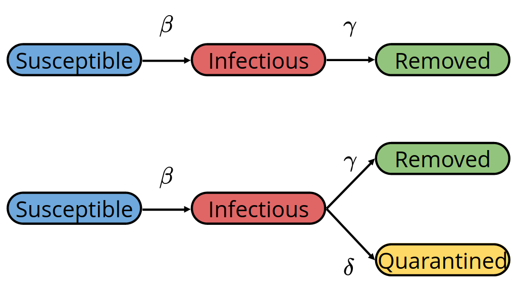
Figure 1: Upper: SIR. Lower: SIRQ.

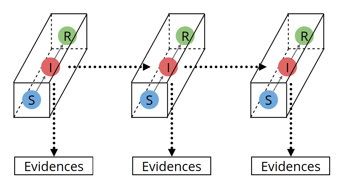
Figure 2: A state-space framework feat. SIR.

SIR, standing for Susceptible-Infectious-Removed, is the basic compartmental model. By using SIR as a stepping stone, we can understand more complex models such as SIRQ, which is promoted as a novel model in this paper.

2.1 SIR model

The SIR model separates the population into three compartments: susceptible, infectious, and removed. Each individual (logically) transfers among these compartments according to his health status (Figure 1).

Susceptible:

The population in this compartment are healthy people who are vulnerable to the disease.

Infectious:

The population in this compartment are infected people who are free to infect those susceptible.

Removed:

This compartment consists of two groups of people – those who died from the disease or recovered from it and hence obtained immunity.

To describe the dynamic governing the mechanism, two types of setups are possible – stochastic or deterministic. The stochastic one assumes that each individual transfers according to some probability. The usual setup is that the probability of a healthy people transferring from susceptible to infectious follows an exponential distribution of parameter $\beta$, and the probability of an infected people transferring from infectious to removed follows an (independent) exponential distribution of parameter $\gamma$.

On the other hand, the deterministic one simplifies the above process by taking advantage of the law of large numbers. Instead of studying the dynamic on an individual basis, the deterministic setup considers it at the aggregate level. That is, the number of individuals in each compartment varies according to some ordinary differential equations (ODE).

Let $S_{t}$, $I_{t}$, and $R_{t}$ be the number of susceptible, infectious, and removed at time $t$, respectively. Let $N_{t}=S_{t}+I_{t}+R_{t}$ be the number of the total population, which is supposed to be constant (i.e., there is no newborn or death owing to reasons other than the infectious disease in question). Then the stochastic dynamic can be expressed by the following equations.

$$\Pr(S_{t+h}-S_{t}=-1,I_{t+h}-I_{t}=1|S_{t},I_{t},R_{t})=\beta S_{t}I_{t}h/N_{t}+o(h),$$

$$\Pr(I_{t+h}-I_{t}=-1,R_{t+h}-R_{t}=1|S_{t},I_{t},R_{t})=\gamma I_{t}h+o(h).$$

The deterministic dynamic can be expressed by the following ODE.

$$\frac{\mathop{}\!\mathrm{d}S_{t}}{\mathop{}\!\mathrm{d}t}=-\frac{\beta S_{t}I_{t}}{N_{t}},$$

$$\frac{\mathop{}\!\mathrm{d}I_{t}}{\mathop{}\!\mathrm{d}t}=\frac{\beta S_{t}I_{t}}{N_{t}}-\gamma I_{t},$$

$$\frac{\mathop{}\!\mathrm{d}R_{t}}{\mathop{}\!\mathrm{d}t}=\gamma I_{t}.$$

For large-scale epidemics, the deterministic dynamic is a good enough approximation of the stochastic dynamic (Kurtz, 1981). Interested readers are also referred to Siettos and Russo (2013, p. 301) for a quick review and to Birrell et al. (2018, Section 3.2) for a detailed discussion.

The parameter $\beta$ is called the transmission rate, and $\gamma$ is called the removal rate. The ratio $\beta/\gamma$ is associated with the most crucial quantity of infectious diseases, the basic reproduction number $\mathcal{R}_{0}=\frac{\beta}{\gamma}$, which stands for the average number of victims an infectious is expected to infect at the very beginning of the outbreak. If $\mathcal{R}_{0}>1$, the disease becomes an epidemic; if $\mathcal{R}_{0}<1$, the disease dies out; if $\mathcal{R}_{0}=1$, it is an endemic (i.e., the number of infectious neither grows nor deceases).

2.2 SIRQ model

There are many extensions to SIR. Here, we design another one, dubbed susceptible-infectious-removed-quarantined (SIRQ), to include the influence of public interventions. SIRQ creates a fourth compartment, quarantined, which hosts the part of infectious getting quarantined or hospitalized (Figure 1). Therefore, the infectious can have two futures: either they stay wild and get nature-selected (i.e., removed) as in the SIR model, or they get quarantined, which prevents them from infecting others all the same.

The dynamics of SIRQ are very similar to the above, so we present here only the deterministic one.

$$\frac{\mathop{}\!\mathrm{d}S_{t}}{\mathop{}\!\mathrm{d}t}=-\frac{\beta S_{t}I_{t}}{N_{t}},$$

$$\frac{\mathop{}\!\mathrm{d}I_{t}}{\mathop{}\!\mathrm{d}t}=\frac{\beta S_{t}I_{t}}{N_{t}}-\gamma I_{t}-\delta I_{t},$$

$$\frac{\mathop{}\!\mathrm{d}R_{t}}{\mathop{}\!\mathrm{d}t}=\gamma I_{t},$$

$$\frac{\mathop{}\!\mathrm{d}Q_{t}}{\mathop{}\!\mathrm{d}t}=\delta I_{t},$$

where $Q_{t}$ is the number of quarantined at time $t$, $N_{t}=S_{t}+I_{t}+R_{t}+Q_{t}$ is the total number of the population, and $\delta$ is the rate the infectious getting quarantined. The ratio $\gamma/\delta$ reflects the ratio of the infectious staying under the radar. Here, the quarantined are assumed not infectious (we consider the possibility of infecting healthcare personnel to be neglectable). Also, we do not further specify the outflow of the quarantined compartment, so it contains three types of people – those being quarantined, those who died during the quarantine, and those who recovered during the quarantine.

This model is particularly relevant to the situation of COVID-19. On the one hand, many victims of COVID-19 are asymptomatic. They will hence not go to the hospital, and they get recovered all by themselves. On the other hand, given the high transmissibility of COVID-19, there are not enough hospital resources for every patient. Many infectious have to stay wild and get nature-selected. Besides the above two reasons, there is another one specific to China, mainland: the recall of the test kits is unsatisfying.

One usage of this model is to speculate the ratio of asymptomatic patients or the ratio of hospitalization. The removed compartment is supposed to be unobservable, whilst the quarantined compartment can be observed from the confirmed cases. Our experiments show that, in the parametric setting, the ratio of asymptomatic patients or the like can be accurately inferred given only sparse information on the infectious and the quarantined.

Concerning the basic reproduction number, it has two choices. The controlled version uses $\frac{\beta}{\gamma+\theta}$, whose value determines whether the disease will become an epidemic or die out. The uncontrolled version uses $\frac{\beta}{\gamma}$, which stands for the outcome if the quarantine measure is ever called off.

3 State-space framework

The state-space framework has become the de facto state of the art for the usage of compartment models. Many studies, such as the one by Wu et al. (2020), use this framework implicitly. This section will first lay down a solid mathematical foundation of the state-space framework and then complement it with some concrete examples.

3.1 Mathematical foundation

The state-space framework is very similar to the Hidden Markov Model in machine learning. It assumes that the compartment status is in the invisible state space and that we can only observe secondary information derived from the states. Let us illustrate this concept with SIR. The vector $(S_{t},I_{t},R_{t})$ forms the (invisible) state at time $t$. The dynamic characterized by the parameters $(\beta,\gamma)$ connects the temporally successive states (e.g., $(S_{t},I_{t},R_{t})$ and $(S_{t+1},I_{t+1},R_{t+1})$). The state at time $t$ determines the evidence data that we could collect at time $t$ (Figure 2).

In the state-space framework, there are usually two tasks. The first one is to infer the underlying state status, which tells us the severity of the current epidemic. The second one is to characterize the properties (e.g., $\mathcal{R}_{0}$) of the epidemic itself, which helps us evaluate the ferocity of our enemy. These two tasks are interdependent: the fulfillment of one entails the other.

It is a principled way to infer these two tasks together through the graphical model (Figure 3). First of all, the epidemic dynamic parameter $\theta$ (in SIR, $\theta=(\beta,\gamma)$) governs the temporal transition of the states $X_{t}$ (in SIR, $X_{t}=(S_{t},I_{t},R_{t})$):

$$X_{t+1}|X_{t}\sim p_{\theta}(\cdot|X_{t})\quad\text{(state equation)}.$$

This probability distribution can be degenerate, in which case it is reduced to a deterministic epidemic dynamic. SIR and SIRQ provide examples of $p_{\theta}$. Next, the invisible states $X_{t}$ generates some empirical evidence, denoted as $Y_{t}$:

$$Y_{t}|X_{t}\sim p_{\bar{\eta}}(\cdot|X_{t})\quad\text{(observation equation)},$$

where $\bar{\eta}$ is often manually selected by the researchers to prevent any unintended complexity. Also, Bayesian statisticians may go further by supposing that the parameter $\theta$ lies in some probability space. Thus, they will include in the model a prior:

$$\theta\sim\bar{\pi}(\cdot)\quad\text{(prior)},$$

where the prior $\bar{\pi}$ is preset. Finally, to infer the state $X_{t}$ and the parameter $\theta$, we can build their posterior distribution, which is proportional to the joint distribution. Let $x_{i}$ be the value observed of $X_{i}$ and let $x_{1:T}$ denote the tuple $x_{1},\ldots,x_{T}$, then the posterior distribution

$$p(\theta,x_{1:T}|y_{1:T})\propto p_{\bar{\eta}}(y_{1:T}|x_{1:T})p_{\theta}(x_{1:T})\bar{\pi}(\theta)\quad\text{(posterior)}.$$

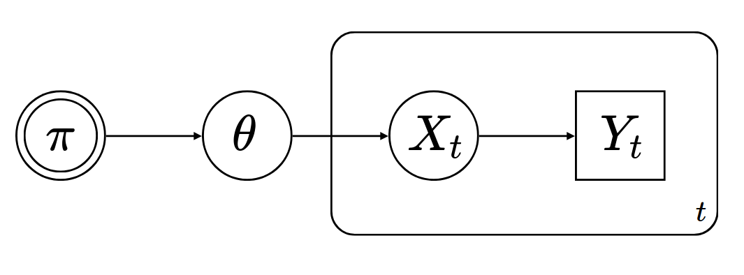
Figure 3: Graphical model for the state-space framework.

The above assumes the Markov property. In practice, the state-space framework can be more general by abandoning the Markov property or by introducing dependence between $Y_{t}$.

In the following, we will give some concrete examples. Section 3.2 gives some candidates for the observation equation, and Section 3.3 gives some candidates for the prior. As for the state equation, SIR and SIRQ in the previous section are good candidates.

3.2 Candidates for the observation equation

The observation equation introduces evidence for the inference of the dynamic and the latent states. Traditionally we use only surveillance data, but now an increasing number of studies start to use exotic data such as serological, demographic, administrative, environmental, and phylogenetic data (Birrell et al., 2018).

The first example is how researchers used traveling data to infer the total number of COVID-19 patients in Wuhan, China. In January 2020, there are a large number of people infected by COVID-19 in Wuhan city. Unaware of the infection, they traveled abroad and later got diagnosed. Imai et al. (2020) modeled this natural experiment as sampling with replacement. That is, the number of patients diagnosed abroad follows a binomial distribution $\text{Bin}(m,I/N)$, where $m$ stands for the total number of outbound travelers, $I$ the number of infectious, and $N$ the total population. Rigorously speaking, the natural experiment is more like sampling without replacement, but the difference is neglectable when $m\ll N$. Wu et al. (2020) modeled it, alternatively, as a Poisson distribution $\text{Poi}(mI/N)$. Incidentally, there is no fundamental difference between the above two options, for $\text{Bin}(m,I/N)\approx\text{Poi}(mI/N)$ when $m>20$ and $I\ll N$ thanks to the law of rare events.

The second example is based on a probably unpopular opinion: using the number of confirmed cases to infer the quarantined compartment. It is attempting to use the confirmed cases for the infectious compartment instead. Nonetheless, a smarter and more sensible arrangement is to use them for the removed compartment in SIR or the quarantined compartment in SIRQ. When a person is confirmed infected, he most likely will be admitted to the hospital and thus lose the ability to infect others (if the risk of infecting the healthcare personnel is low). The removed compartment in SIR is used for this purpose. If the hospitalization is imperfect (i.e., a part of patients are not confirmed and have to be nature-selected), this is a perfect scenario for the SIRQ model, where the confirmed cases can be associated with the quarantined compartment. Xu et al. (2016, Section 5.2) thought alike and used the confirmed cases to infer the removed compartment. In this article, we will use the confirmed cases for the quarantined compartment. The observation equation can either feature the Gaussian distribution or the Poisson distribution. In fact, there is no significant difference, as $\texttt{Poi}(\lambda)\approx\mathcal{N}(\lambda,\lambda)$ for sufficiently large $\lambda$.

The third example is to use the serological data to infer the removed compartment by detecting the antibody in the blood. In an imperfect quarantine scenario modeled by SIRQ, some patients survived the disease without formal medical intervention or died because of it. These patients are never administratively confirmed, but they reflect the severity of the epidemic all the same. To fairly evaluate the epidemic, it is essential to estimate the portion of unconfirmed cases. Since recovered people will have an antibody in the blood, the serological data can help us screen out this group of people. To get an unbiased estimate, we can sample the whole population, and then it is reduced to an elementary statistics problem.

3.3 Candidates for the prior

The prior denotes the preset distribution on the parameter characterizing the dynamic (the parameter characterizing the observation equation is preset). This parameter can be finite-dimensional (vector) or infinite-dimensional (function). The finite-dimensional cases usually use an uninformative prior (i.e., constant), and the posterior degenerates to the plain likelihood. It is only in the infinite-dimensional cases that the selection of prior becomes nontrivial.

In the infinite-dimensional case, the parameter $\theta_{t}$ is time-varying. We are to sample functions for $\theta_{t}$ in some function space. In other words, $\theta_{t}$ is a stochastic process. There are mainly two candidate spaces for this purpose. The first defines the stochastic process by a stochastic differential equation:

$$\mathop{}\!\mathrm{d}h(\theta_{t})=\mu_{t,\theta}\mathop{}\!\mathrm{d}t+\sigma_{t,\theta}\mathop{}\!\mathrm{d}B_{t},$$

where $\mu_{t,\theta}$ is the drift, $\sigma_{t,\theta}$ is the volatility, $B_{t}$ is a standard Wiener process, and $h(\cdot)$ is a preset deterministic function. The most common choice for $\theta_{t}$ is Brownian motion where $h(\cdot)=\cdot$ and geometric Brownian motion where $h(\cdot)=\log(\cdot)$. If the process is expected to converge, Dureau, Kalogeropoulos and Baguelin (2013, p. 4) also proposed the Ornstein Uhlenbeck process.

The second function space is the Gaussian process. A Gaussian process has the property that its arbitrary segments follow a multivariate Gaussian distribution, hence the name. It is wildly used in nonparametric Bayesian statistics. The distribution of the Gaussian process is uniquely defined by its expectation (function) and its kernel (covariance function) $K(\cdot,\cdot)$. Xu et al. (2016) investigated two types of kernels: squared exponential

$$K(x,y)=\alpha^{2}\exp[-(x-y)^{2}/(2\ell^{2})]$$

and periodic

$$K(x,y)=\alpha^{2}\exp(-\ell^{-1}(1-\cos(2\pi\omega^{-1}|x-y|))).$$

In the above description, the parameter $\theta_{t}$ is quite abstract. In practice, this $\theta_{t}$ has concrete meanings. For example, in SIRQ, $\theta_{t}=(\beta_{t},\gamma_{t},\delta_{t})$, in which case, we can apply independent priors individually on each component.

4 Total variation regularization and Iterated Nelder–Mead

Priors can limit the model complexity and hence control the model estimation error in the context of bias-variance tradeoff. An alternative approach is to apply a regularization on the log-likelihood. This section introduces the concept of total variation regularization, which is popular in image denoising. It has the advantage of detecting the discontinuities in the investigated object, and thus it is expected here to capture sudden shocks on the dynamics. Also, in contrast to Monte Carlo methods, the standard approach to calculate the posterior mean, this section designs a novel algorithm, dubbed Iterated Nelder–Mead, intended to calculate the posterior mode.

4.1 Total variation regularization

Section 3 formulates the posterior as

$$p_{\bar{\eta}}(y_{1:T}|x_{1:T})p_{\theta}(x_{1:T})\bar{\pi}(\theta).$$

By applying logarithm, we get

$$\underbrace{\log p_{\bar{\eta}}(y_{1:T}|x_{1:T})+\log p_{\theta}(x_{1:T})}_{\text{log-likelihood}}+\underbrace{\log\bar{\pi}(\theta)}_{\text{regularization}},$$

where the last term can be regarded as a regularization. In other words, prior is one type of regularization.

An alternative regularization would be substituting the prior for a norm applied on $\theta$:

$$\underbrace{\log p_{\bar{\eta}}(y_{1:T}|x_{1:T})+\log p_{\theta}(x_{1:T})}_{\text{log-likelihood}}+\underbrace{\left\lVert\theta\right\rVert}_{\text{regularization}}.$$

This norm can be, among others, total variation

$$\left\lVert\theta\right\rVert_{\text{TV}}:=\sup\sum_{i}|\theta_{t_{i+1}}-\theta_{t_{i}}|,$$

where the supreme runs over the set of all partitions, or quadratic variation

$$[\theta]:=\lim_{\left\lVert P\right\rVert\rightarrow 0}\sum_{i}(\theta_{t_{i+1}}-\theta_{t_{i}})^{2},$$

where $P$ ranges over all partitions and the norm is the mesh.

The above frames the prior as a type of regularization; the converse is true as well. Total variation regularization or quadratic variation regularization can be regarded as a prior on the space of functions with finite total variations or finite quadratic variations, respectively. In particular, quadratic variation regularization is equivalent to specifying $\theta$ as Brownian motion.

4.2 Iterated Nelder–Mead

It is wildly perceived, in the computer vision community, that the posterior mean’s ability to recover the discontinuity is not as good as the posterior mode. This subsection describes the challenges to calculate the posterior mode as well as provides solutions to it.

The first challenge is the unavailability of the gradient. Although the part of the likelihood associated with the observation equation can be easily differentiated, the part associated with the state equation does not have closed-forms. Therefore, we have to rely on some zero-order algorithm. One algorithm fit for this purpose is the Nelder–Mead method (a.k.a. downhill simplex method), which is prevalent in civil engineering. For example, to build a suspension bridge, an engineer has to choose the thickness of each strut, cable, and pier. These elements are interdependent, and it is not easy to determine the impact of changing any specific element. Analogously, in our context, changing the value of the dynamic at any single point is unlikely to have a significant impact on the whole epidemic (the integral does not depend on the function values on a null set).

The second challenge is the multimodality of the objective function, which refers to functions with multiple modes. Two factors contribute to this multimodality. On the one hand, when the observation is sparse, there are many candidate dynamics able to reproduce the observation accurately; each candidate then forms a valley. On the other hand, constant dynamics do not suffer from the regularization penalty, and the modification on a single point will not affect the overall dynamic (null set) but does increase total variation, so each constant dynamic also forms a valley. The optimization algorithm can, therefore, be easily trapped in some local optimum. To mitigate the influence of multimodality, we designed the Iterated Nelder–Mead algorithm, which repeatedly reruns Nelder–Mead on the new local optimum. (Algorithm 1).

Algorithm 1 Iterated Nelder–Mead

initiate point x, objective function f

repeat

     $\textbf{x}\leftarrow\text{Nelder--Mead}(\textbf{f},\textbf{x})$

until stop condition fulfilled

Iterated Nelder–Mead mitigates the problem of multimodality to some extent, but it does not affect the hardship of the problem itself. During the experiments, we discovered that the regularization hyperparameter (weight) plays a critical role in defining the hardship of the problem by altering the topology of the objective function. Indeed, when the regularization weight is small, the objective function has many equally good local minima—the desired local minimum hides among its peers. When the regularization weight is large, the objective function contains fewer local minima with each minimum, however, being an abyss. Once the solver loses its way into one abyss, it has no chance ever to escape. Therefore, the regularization weight should be something in-between—highlight the desired local minimum while preserving the smoothness of the objective function (Figure 4).

Figure 4: Topology of the objective function with various regularization weights. Left: under-regularized. Middle: over-regularized. Right: well-regularized.

5 Experiments

Three types of dynamics and three types of (simulated) data are investigated in this study. The three types of dynamics are constant SIRQ with no regularization, time-varying SIR with regularization, and time-varying SIRQ with regularization. All dynamics use the ODE versions specified in Section 2 and are implemented with the Euler-Maruyama scheme.

The three types of data are virulence data, surveillance data, and serology data:

Virulence.

Sample the population and test for the pathogen (e.g., virus). This data is for the estimation of the current number of infectious people

Surveillance.

The confirmed and thus quarantined cases of the disease. This data is for the estimation of the number of removed (in SIR) or quarantined (in SIRQ) people.

Serology.

Sample the population and test for the antibody. This data is for the estimation of the removed people in SIRQ provided that the infectious disease in question is a novel one. If the sampling cost is a concern, this data can be collected along with the virulence data.

5.1 Constant SIRQ

The SIRQ model has three parameters $\theta=(\beta,\gamma,\delta)$. The epidemic takes place in a small town with 1000 inhabitants. It starts with 10 infectious people and 0 removed or quarantined people. Then the epidemic develops with a dynamic $(\beta,\gamma,\delta)=(0.3,0.03,0.07)$. Two types of evidence are available for the inference of the epidemic. The virulence data is 9 samples during the life of the epidemic, with a sample size of 10 people each. The surveillance data is the number of confirmed cases at 8 different moments. The maximum likelihood estimate yields the value $(\hat{\beta},\hat{\gamma},\hat{\delta})=(0.307,0.030,0.073)$, very close to the ground truth.

Although this experiment does not include any time-varying factor, it demonstrates the power of this simple model. With virulence data and surveillance data only, we can precisely estimate the basic reproduction number and the quarantine ratio $\delta/\gamma$. This model is particularly useful in the COVID-19 pandemic, where many victims are asymptomatic.

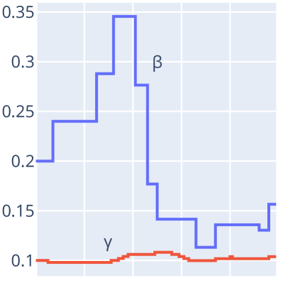
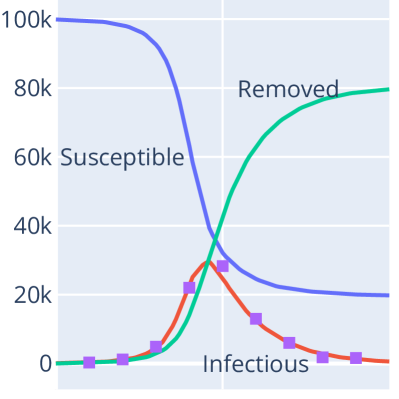
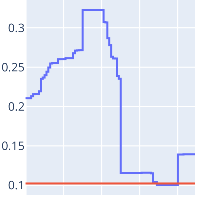
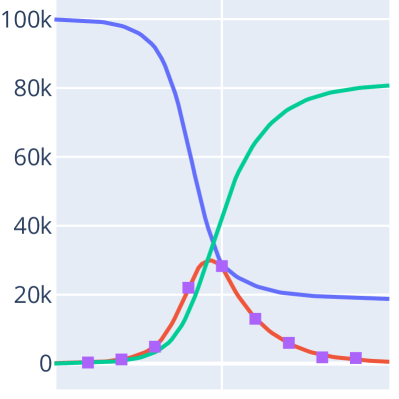
Figure 5: Time-varying SIR. Left: the dynamic. Right: the resulted epidemic and the evidence (represented by the dots). Top: ground truth. Bottom: estimation. $\beta$ denotes the transmission rate; $\gamma$ denotes the removal rate.

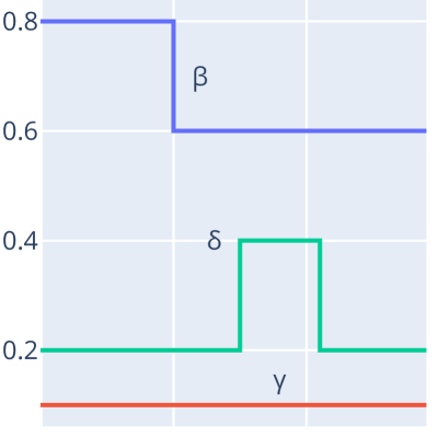
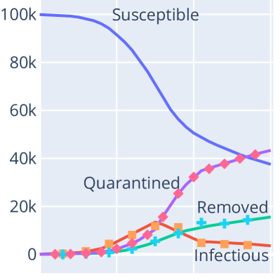
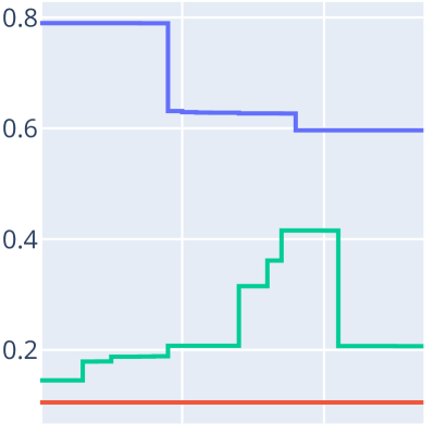
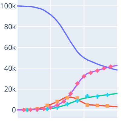
Figure 6: Time-varying SIRQ. Left: the dynamic. Right: the resulted epidemic and the evidence (dots). Top: ground truth. Bottom: estimation. $\beta$ denotes the transmission rate; $\gamma$ denotes the removal rate; $\delta$ denotes the quarantine rate.

5.2 Time-varying SIR with regularization

The model tested in this subsection has one time-varying parameter and one constant parameter $\theta_{t}=(\beta_{t},\gamma)$. The transmission rate $\beta_{t}$ is supposed to be time-varying to reflect, among others, the gatherings in holidays, the adoption of social distancing. The removal rate $\gamma$ is supposed to be constant because the aggressiveness of the virus and the resistance of the population are believed to be stable (unless the virus mutates). In the experiment, the ground truth $\beta_{t}$ firstly increases because of holiday gatherings. It then drops because of increasing public awareness (Figure 5).

The epidemic takes place in a city of 100k inhabitants. It starts with 100 infectious people and 0 removed people. The only data available to infer the epidemic is the 9-sample virulence data during the life of the epidemic, with each sample containing 1k people. The lack of the number of confirmed cases suggests that this is a foreign country trying to evaluate an epidemic-struck country with information censorship; the virulence data corresponds to the exported cases.

The data is considered sparse in contrast to the 100-dimensional parameter, which justifies the necessity of regularization. We applied total variation regularization and solved it with Iterated Nelder–Mead. The estimated dynamic qualitatively recovers the ground truth and generates evidence identical to the sample collected (Figure 5).

5.3 Time-varying SIRQ with regularization

The model tested in this subsection has two time-varying parameters and one constant parameter $\theta_{t}=(\beta_{t},\gamma,\delta_{t})$. The transmission rate $\beta_{t}$ is supposed to be time-varying to reflect, among others, the gatherings in holidays, the adoption of social distancing. The removal rate $\gamma$ is supposed to be constant because the aggressiveness of the virus and the resistance of the population are believed to be stable (unless the virus mutates). The quarantine rate $\delta_{t}$ is supposed to be time-varying to reflect the opening of field hospitals. In the experiment, the ground truth $\beta_{t}$ is mostly constant with one sudden drop because of the city lockdown, whilst the ground truth $\delta_{t}$ rises suddenly thanks to the opening of a field hospital and then drops to the previous level because the hospital is full (Figure 6).

The epidemic takes place in a city of 100k inhabitants. It starts with 100 infectious people and 0 removed or quarantined people. The data available here is much richer than the scenario in the last subsection. It includes a 9-sample virulence data with each containing 1k people, the confirmed cases, and a 9-sample serology data with each also containing 1k people. All this information is not too difficult to obtain for countries with excellent governance.

One challenge to infer this model is the coexistence of two time-varying parameters. Still, total variation regularization and Iterated Nelder–Mead succeeded in reproducing the ground truth, and the estimated dynamic generates evidence that perfectly fits the reality.

6 Conclusions

The combination of total variation regularization and Iterated Nelder–Mead successfully detects the discontinuities of the underlying time-varying dynamics. When the epidemic follows an SIR dynamic with time-varying transmission rate $\beta_{t}$, the proposed combination recovers the dynamic with the help of sparse virulence data. When the epidemic follows an SIRQ dynamic with time-varying transmission rate $\beta_{t}$ and time-varying quarantine rate $\delta_{t}$, the proposed combination recovers the dynamic with the help of virulence, surveillance, and serology data.

There are three directions to strengthen this study. Firstly, it is unclear whether the local optimum achieved by Iterated Nelder–Meadis the global one. Since the optimization algorithm plays a crucial role in the solution-finding process, one part of the research effort should be improving the searching ability of the optimization algorithm. Secondly, it is currently unclear whether these dynamics could be perfectly recovered with more data or under better conditions. One research direction thus consists of precisely inferring the underlying dynamics so that public policies (e.g., city lockdown) could be better evaluated. It also helps compare the efficiency of different policies in the same country and the efficiency of the same policy in different countries. Thirdly and most importantly, we believe that our machinery is a handy weapon against COVID-19.

References

- (1)
- Althaus (2014) Althaus, C. L. (2014), ‘Estimating the reproduction number of ebola virus (ebov) during the 2014 outbreak in west africa’, PLoS currents 6.
- Birrell et al. (2018) Birrell, P. J., De Angelis, D. and Presanis, A. M. (2018), ‘Evidence synthesis for stochastic epidemic models’, Statistical Science 33(1), 34–43.
- Camacho et al. (2014) Camacho, A., Kucharski, A., Funk, S., Breman, J., Piot, P. and Edmunds, W. (2014), ‘Potential for large outbreaks of ebola virus disease’, Epidemics 9, 70–78.
- Cazelles et al. (2018) Cazelles, B., Champagne, C. and Dureau, J. (2018), ‘Accounting for non-stationarity in epidemiology by embedding time-varying parameters in stochastic models’, PLoS computational biology 14(8).
- Chowell et al. (2004) Chowell, G., Hengartner, N. W., Castillo-Chavez, C., Fenimore, P. W. and Hyman, J. M. (2004), ‘The basic reproductive number of ebola and the effects of public health measures: the cases of congo and uganda’, Journal of theoretical biology 229(1), 119–126.
- Dureau, Ballesteros and Bogich (2013) Dureau, J., Ballesteros, S. and Bogich, T. (2013), Ssm: Inference for time series analysis with state space models.
- Dureau, Kalogeropoulos and Baguelin (2013) Dureau, J., Kalogeropoulos, K. and Baguelin, M. (2013), ‘Capturing the time-varying drivers of an epidemic using stochastic dynamical systems’, Biostatistics 14(3), 541–555.
- Funk et al. (2018) Funk, S., Camacho, A., Kucharski, A. J., Eggo, R. M. and Edmunds, W. J. (2018), ‘Real-time forecasting of infectious disease dynamics with a stochastic semi-mechanistic model’, Epidemics 22, 56–61.
- Funk et al. (2017) Funk, S., Ciglenecki, I., Tiffany, A., Gignoux, E., Camacho, A., Eggo, R. M., Kucharski, A. J., Edmunds, W. J., Bolongei, J., Azuma, P. et al. (2017), ‘The impact of control strategies and behavioural changes on the elimination of ebola from lofa county, liberia’, Philosophical Transactions of the Royal Society B: Biological Sciences 372(1721), 20160302.
- He et al. (2011) He, D., Dushoff, J., Day, T., Ma, J. and Earn, D. J. (2011), ‘Mechanistic modelling of the three waves of the 1918 influenza pandemic’, Theoretical Ecology 4(2), 283–288.
- Imai et al. (2020) Imai, N., Dorigatti, I., Cori, A., Donnelly, C., Riley, S. and Ferguson, N. (2020), ‘Report 2: Estimating the potential total number of novel coronavirus cases in wuhan city, china’.
- Kermack and McKendrick (1927) Kermack, W. O. and McKendrick, A. G. (1927), ‘A contribution to the mathematical theory of epidemics’, Proceedings of the royal society of london. Series A, Containing papers of a mathematical and physical character 115(772), 700–721.
- Kucharski et al. (2020) Kucharski, A. J., Russell, T. W., Diamond, C., Liu, Y., Edmunds, J., Funk, S., Eggo, R. M., Sun, F., Jit, M., Munday, J. D. et al. (2020), ‘Early dynamics of transmission and control of covid-19: a mathematical modelling study’, The lancet infectious diseases .
- Kurtz (1981) Kurtz, T. G. (1981), Approximation of population processes, Vol. 36, SIAM.
- Rasmussen et al. (2011) Rasmussen, D. A., Ratmann, O. and Koelle, K. (2011), ‘Inference for nonlinear epidemiological models using genealogies and time series’, PLoS computational biology 7(8).
- Siettos and Russo (2013) Siettos, C. I. and Russo, L. (2013), ‘Mathematical modeling of infectious disease dynamics’, Virulence 4(4), 295–306.
- Smirnova et al. (2019) Smirnova, A., deCamp, L. and Chowell, G. (2019), ‘Forecasting epidemics through nonparametric estimation of time-dependent transmission rates using the seir model’, Bulletin of mathematical biology 81(11), 4343–4365.
- Stocks et al. (2018) Stocks, T., Britton, T. and Höhle, M. (2018), ‘Model selection and parameter estimation for dynamic epidemic models via iterated filtering: application to rotavirus in germany’, Biostatistics .
- Wu et al. (2020) Wu, J. T., Leung, K. and Leung, G. M. (2020), ‘Nowcasting and forecasting the potential domestic and international spread of the 2019-ncov outbreak originating in wuhan, china: a modelling study’, The Lancet 395(10225), 689–697.
- Xu et al. (2016) Xu, X., Kypraios, T. and O’Neill, P. D. (2016), ‘Bayesian non-parametric inference for stochastic epidemic models using gaussian processes’, Biostatistics 17(4), 619–633.