A Consistency Test of EFT Power Countings from Residual Cutoff Dependence

Abstract

I summarise a method to quantitatively assess the consistency of power-counting proposals in Effective Field Theories which are non-perturbative at leading order. It uses the fact that the Renormalisation Group evolution of an observable predicts the functional form of its residual cutoff dependence on the breakdown scale of an Effective Field Theory (EFT), on the low-momentum scales, and on the order of the calculation. Passing this test is a necessary but not sufficient consistency criterion for a suggested power counting whose exact nature is disputed. For example, in Chiral Effective Field Theory ($\chi$EFT) with more than one nucleon, a lack of universally accepted analytic solutions obfuscates the relation between convergence pattern and numerical results, and led to proposals which predict different numbers of Low Energy Coefficients (LECs) at the same chiral order, and at times even predicts a different ordering long-range contributions. The method may provide an independent check whether an observable is properly renormalised at a given order, and allows one to estimate both the breakdown scale and the momentum-dependent order-by-order convergence pattern of an EFT. Conversely, it may help identify those LECs (and long-range pieces) which produce renormalised observables at a given order. I also discuss its underlying assumptions and relation to the Wilsonian Renormalisation Group Equation; useful choices for observables and cutoffs; the momentum window in which the test likely provides best signals; its dependence on the values and forms of cutoffs as well as on the EFT parameters; the impact of fitting LECs to data in different or the same channel; and caveats as well as limitations. Since the test is designed to minimise the use of data, it allows one to quantitatively falsify if the EFT has been renormalised consistently. This complements other tests which quantify how an EFT compares to experiment. Its application in particular to the ${}^{3}\mathrm{P}_{0}$ and ${}^{3}\mathrm{P}_{2}$-${}^{3}\mathrm{F}_{2}$ partial waves of $\mathrm{NN}$ scattering in $\chi$EFT may elucidate persistent power-counting issues.

1 Motivation: Serious Theorists Have Error Bars

1.1 Introduction

That our understanding of natural phenomena is based on concrete, falsifiable predictions is deeply ingrained in the scientific method. It is insufficient to compare numbers; one also must judge their reliability. And since we do not trust experiments without error bars, why should it be acceptable for a theorist to not assess uncertainties in a calculation, before a closer look at the data to be explained? Simply stating that this is “difficult” is certainly no sufficient excuse, especially after the recent surge of articles which offer statistically meaningful methods to ascertain and interpret theory errors; see e.g. editorial ; JPhysG ; JPhysG2 . The prospect of a reproducible, objective, quantitative estimate of theoretical uncertainties lies thus at the heart not only of any Effective Field Theory (EFT). But EFTs claim to possess well-defined schemes to find just such estimates. It is therefore befitting to explore how the validity of such prescriptions can be gauged.

More than two decades ago, Lepage discussed in a highly influential lecture methods to quantify convergence to data Lepage:1997cs , no doubt based on standard lore in Computational Physics (see e.g. Ref. Landau ). In contradistinction, the test presented in the following hopes to quantify the internal consistency of an EFT and takes minimal resort to experimental information. In an ideal world, theorists would perform “double-blind” calculations in which theoretical uncertainties are assessed under the pretence that no or only very limited data is available. Such “post-dictions” are of course predictions when information is indeed experimentally unknown or hard to access, or when data consistency must be checked. But even when not, they contribute to the discourse and hopefully increase the community’s confidence in the method used. They thus form an important sociological aspect of the Scientific Method.

The presentation is organised as follows. The remainder of this Introduction aims to motivate why a reliable scheme to quantify theory uncertainties is imperative but not quite straightforward in EFTs with unnatural shallow scales, and lists schemes discussed in the literature. Section 2 provides a first description of the proposed test, on a rather abstract level. An example in sect. 3 provides a concrete experience of the method. After this illustration, the final section addresses a number of what may at first reading be perceived as details. Most of these are cross-referenced in sect. 2, so that the interested reader can quickly find further information if desired. These topics include: extensions, assumptions, choices, and limitations of the method; a discussion of which observables and kinematics are likely to provide clear signals; and miscellaneous notes; followed by concluding remarks. This organisation has the advantage to not overburden the initial presentation in sect. 2 with a large numbers of qualifiers and footnotes which disrupt the flow.

On a historical note, the origin of these remarks goes back to publications in 2003 and 2005 Bedaque:2002yg ; improve3body , and to lectures at the 2008 US National Nuclear Physics Summer School NNPSS . When the issue was revisited at two workshops Saclay ; Benasque , its conclusions were generally perceived as not immediately straightforward or widely known. Input on some aspects was also provided for two recent publications Furnstahl:2014xsa ; Epelbaum:2014efa . Dai et al. explored it in $\overline{\mathrm{N}}\mathrm{N}$ scattering Dai:2017ont . It seems therefore fitting to present an expanded Technical Note, updating, expanding and – where necessary – correcting a proceeding from 2015 Griesshammer:2015osb .

1.2 Rationale: Consistency Issues in EFTs with Shallow Bound States

Effective Field Theories take advantage of a separation of scales to expand interactions and observables in a dimension-less quantity which for the sake of this presentation is denoted by

$$Q=\frac{\text{typical low momenta }k,p_{\text{typ}}}{\text{breakdown scale }\overline{\Lambda}_{\text{EFT}}}<1\;\;.$$ (1)

The numerator contains the relative momentum $k$ between scattering particles, and other intrinsic low scales which are summarily denoted by $p_{\text{typ}}$. At the breakdown scale $\overline{\Lambda}_{\text{EFT}}$, new dynamical degrees of freedom enter which are not explicitly accounted for by the EFT but whose effects at these short distances are simplified into Low-Energy Coefficients (LECs).

Consider, for example, Chiral Effective Field Theory ($\chi$EFT), the extension of (purely mesonic) Chiral Perturbation Theory to the one- and few-nucleon system; see e.g. Hammer:2019poc for a recent review: $p_{\text{typ}}$ then includes the pion mass and the inverse scattering lengths of the $\mathrm{NN}$ system: $\gamma_{t}\approx 45\;\mathrm{MeV}$ in the ${}^{3}\mathrm{S}_{1}$ channel and $\gamma_{s}\approx-8\;\mathrm{MeV}$ in the ${}^{1}\mathrm{S}_{0}$ channel are at leading order given by the inverse scattering lengths of these channels, $\gamma_{t,s}\approx 1/a_{t,s}$. Its breakdown scale $\overline{\Lambda}_{\chi}\approx[700\dots 1000]\;\mathrm{MeV}$ is consistent with the masses of the $\omega$ and $\rho$ as the next-lightest exchange mesons, and with the chiral symmetry breaking scale – if the $\Delta(1232)$ as lowest nucleonic resonance is included as dynamical degree of freedom. In a theory without it, the breakdown scale shrinks to $\overline{\Lambda}_{\chi}(\not{\Delta})\approx 300\;\mathrm{MeV}$. Another example is “pion-less EFT” (EFT($\not{\pi}$)), which in turn is the low-energy version of $\chi$EFT because the pion itself is integrated out, so that $\overline{\Lambda}_{\not{\pi}}\approx m_{\pi}\gg p_{\text{typ}}\sim\gamma_{t,s}$. With such a parameter, all interactions and contributions to any observable are determined by expanding them in $Q$ and estimating their relative strengths by Naïve Dimensional Analysis NDA ; NDA2 ; Weinberg:1989dx ; Georgi:1992dw ; Griesshammer:2005ga . When all interactions are perturbative, as in the mesonic and one-baryon sectors, this amounts to not much more than counting powers of $k$ and $p_{\text{typ}}$ – hence the name power counting (PC) scheme.

The situation is more complicated when some interactions must be treated non-perturbatively at leading order because of shallow real or virtual bound states with scales $p_{\text{typ}}\ll\overline{\Lambda}_{\text{EFT}}$ in the EFT’s range of validity. In $\mathrm{NN}$ scattering, all terms in the leading-order (LO) Lippmann-Schwinger equation, including the potential, must be of the same order when all nucleons are close to their non-relativistic mass-shell. If that were not the case, one term could be treated as perturbation of the others and there would be no shallow bound-state. Thus, a shallow bound state necessitates resumming at least some particular interaction or interactions, i.e. an infinite number of interaction points at LO. This, in turn, imposes a consistency condition on that interaction and on the amplitude. In a non-relativistic theory, both the amplitude $T_{\mathrm{NN}}$ and potential $V_{\mathrm{NN}}$ must be of order $Q^{-1}$.

In order to show this, consider the intermediate-state $\mathrm{NN}$ propagator (correlated Green’s function) $G_{\mathrm{NN}}\propto\frac{1}{\vec{q}^{2}-\vec{k}^{2}}$ in time-ordered perturbation theory, where $\vec{q}$ is the relative momentum of one nucleon in the intermediate state, and $\vec{k}$ is the scattering momentum. In a field-theoretical approach, $G_{\mathrm{NN}}$ emerges after one picks the nucleon-pole in the (non-relativistic) energy-integration, $q_{0}\sim\frac{q^{2}}{2M}$ (“potential” régime; see e.g. Beneke:1997zp ; Griesshammer:1997wz ). In either case, the integral is dominated by momenta $k\sim q$.

Denoting $T_{\mathrm{NN}}$ by an ellipse and $V_{\mathrm{NN}}$ by a rectangle, one arrives at the semi-graphical equation:

$$\begin{split}\includegraphics[clip={},width=433.62pt]{consistentPC-onecolumn.pdf}\end{split}$$ (2)

Therefore, a shallow real or virtual bound state mandates $T_{\mathrm{NN}}\sim V_{\mathrm{NN}}\sim Q^{-1}$, unless one is willing to resort to ad-hoc fine-tuning between differing contributions.

This leads to a surprising take on the one-pion exchange. It appears to scale as $(\vec{\sigma}_{1}\cdot\vec{q})(\vec{\sigma}_{2}\cdot\vec{q})/(\vec{q}^{2}+m_{\pi}^{2})\sim Q^{0}$ when one counts only explicit low-momentum scales, but must be of order $Q^{-1}$ if its iteration is to be mandated in bound-state dynamics $q_{0}\sim\frac{q^{2}}{2M}$. For $q_{0}\sim q$, on the other hand, the nucleon becomes static, $\mathrm{NN}$ rescattering is suppressed, and one enters the soft and ultra-soft régimes of Non-Relativistic QED/QCD; see e.g. Refs. Beneke:1997zp ; Griesshammer:1997wz and references both in and to these.

In a straightforward extension, amplitude and interaction between $n$ nucleons which accommodate non-perturbative features at LO scale as

$$T_{n\mathrm{N}}\sim V_{n\mathrm{N}}\sim Q^{1-n}\;\;.$$ (3)

Since both the interactions and the LECs themselves carry inverse powers of $Q$, finding their importance by just counting momenta is therefore clearly insufficient.

The resulting scaling for $T_{n\mathrm{N}}$ only assumes the existence (but not particular numerical value) of unnaturally small scales, irrespective of the form of the interaction. It does not reveal which terms constitute the LO potential or how the “unnatural” shallow scale emerges; only how those terms must be power-counted.

These arguments imply that a choice of EFTs exists, all of which have the same symmetries and degrees of freedom but differ in their power counting. These include the popularly used version with shallow $\mathrm{NN}$ bound states and the one-pion exchange at leading order Hammer:2019poc ; a “KSW” version in which the one-pion exchange scales indeed as $Q^{0}$ and thus is not needed to bind the shallow bound states at LO but enters at NLO, with analytic results in the $\mathrm{NN}$ system that pass every test of self-consistency but limit the radius of convergence to $\overline{\Lambda}_{\mathrm{KSW}}\lesssim 200\;\mathrm{MeV}$ or so Kaplan:1998tg ; Kaplan:1998we ; Fleming:1999ee ; and a version in which low-energy Nuclear Physics has no shallow bound states at all ($\gamma_{t,s}\sim\overline{\Lambda}_{\text{EFT}}$), so that the one-pion exchange is perturbative. Nature’s provision of shallow bound states rules out the latter.

In $\mathrm{NN}$ scattering, a main issue appears to be an intrinsic scale $\Lambda_{\mathrm{NN}}=16\pi f_{\pi}^{2}/(g_{A}^{2}M)\approx 300\;\mathrm{MeV}$, where $f_{\pi}\approx 92\;\mathrm{MeV}$ is the pion decay constant and $g_{A}\approx 1.27$. It sets the strength of the one-pion exchange potential Kaplan:1998we ; Barford:2002je and lies right between the typical low scale $m_{\pi}$ and the expected breakdown scale $\overline{\Lambda}_{\chi}$, possibly providing a less-than-perfect separation of scales and convergence.

This behaviour of LO amplitudes and interactions in the presence of shallow bound states has long been recognised in pionless EFT (EFT($\not{\pi}$)) and its variants (like Halo-EFT and EFT of point-like interactions), where the scaling of operators and the $\beta$ functions of couplings between up to $3$ nucleons are well-established Bedaque:2002mn ; Platter:2009gz ; Hammer:2019poc . For example, analytic results in well-controlled limits show one momentum-independent $3\mathrm{N}$ operator at LO. Likewise, Non-Relativistic QED and QCD count the Coulomb potential as $Q^{-1}$ to allow its resummation.

The situation in $\chi$EFT for two and more nucleons is less obvious. In order to circumvent the apparent paradox between having to resum in order to get a shallow bound state on the one hand, and the momentum scaling of the one-pion exchange potential on the other hand, Weinberg pragmatically suggested to still count LECs and the one-pion exchange as $Q^{0}$, but to apply the perturbative counting of momenta not to amplitudes but to the few-nucleon potential, which is then iterated to produce shallow bound states. How this translates into a PC of observables is under dispute. It has also been demonstrated that Weinberg’s pragmatic proposal predicts an incorrect scaling of short-distance singularities with $m_{\pi}$ Beane:2001bc ; and that it permits no unique convergence for $\Lambda\gtrsim\overline{\Lambda}_{\text{EFT}}$, including in the limit $\Lambda\to\infty$ Nogga:2005hy ; see also U. van Kolck’s contribution to this volume vankolck . Further disagreement persists about the interpretation of approximate solutions (large off-shell momenta, semi-classical limit, etc.), and about more technical problems (deeply bound states etc.). In addition, a cutoff/regulator $\Lambda$ becomes numerically necessary. It is conceptually quite different from the breakdown scale $\overline{\Lambda}_{\text{EFT}}$, albeit the two symbols are similar. It cannot be much smaller than the breakdown scale in order not to “cut out” physical, low-resolution momenta in loops. But even how far $\Lambda$ should be varied is under dispute: Is any value $\Lambda\gtrsim\overline{\Lambda}_{\text{EFT}}$ legitimate, including $\Lambda\to\infty$ (see e.g. ref. Nogga:2005hy and references to it); or should the range be constrained to $\Lambda\approx\overline{\Lambda}_{\text{EFT}}$ (see e.g. ref. Epelbaum:2006pt and references to it)?

In any case, it should be clear that no particular value of any cutoff (including infinity) is preferred to any other, as long as $\Lambda\gtrsim\overline{\Lambda}_{\text{EFT}}$. For any cutoff, one truncates some non-physical high-momentum/short-distance modes whose Physics is not represented in detail, just because an EFT’s effective degrees of freedom are ineffective for loop momenta $q\gtrsim\overline{\Lambda}_{\text{EFT}}$.

It is thus no surprise that in addition to Weinberg’s pragmatic proposal, three active PC proposals emerged in $\chi$EFT, all with the same degrees of freedoms: nucleons and pions only Weinberg ; Birse:2005um ; Birse:2009my ; Valderrama:2009ei ; Valderrama:2011mv ; Valderrama:2019lhj ; Long:2011xw ; Long:2012ve . Table 1 lists their predictions for the order at which a LEC or long-range contribution enters in the lower $\mathrm{NN}$ partial waves. While there is agreement that the long-range part is dominated by one-pion-exchange, ordering of its two-pion exchange is under dispute. More importantly, each finds a different number of LECs at any given order – and each claims consistency. Not all can be right, though. Articles, panels and sessions at Chiral Dynamics and other conferences as well as dedicated workshops led to little consensus (see e.g. Daniel Phillips’ even-handed account at Chiral Dynamics 2012 Phillips:2013fia and van Kolck’s more recent review vanKolck:2020llt ); some additional notable contributions include Refs. Kaplan:1996xu ; Kaplan:1998we ; Beane:2001bc ; Nogga:2005hy ; Epelbaum:2006pt ; Beane:2008bt ; Epelbaum:2009sd ; Valderrama:2016koj ; Hammer:2019poc .

This is not just stamp-collecting or a philosophical question which potentially exposes the soft underbelly of $\chi$EFT and the credibility of its error assessments, but which is “otherwise” of little practical consequence. A central EFT promise is that it encodes the unresolved short-distance information at a given accuracy into not just some, but the smallest-possible number of independent LECs under given symmetries. For example, the PC proposals of $\mathrm{NN}$ $\chi$EFT differ most for attractive triplet waves: the ${}^{3}\mathrm{P}_{2}$-${}^{3}\mathrm{F}_{2}$ system at order $Q^{0}$ has no LEC parameter Weinberg – or $3$ of similar size Birse:2005um ; Birse:2009my – or $3$, but with different weights Valderrama:2009ei ; Valderrama:2011mv ; Valderrama:2019lhj – or $1$Long:2011xw ; Long:2012ve . To bring it to a boil: If all proposals are renormalised and fit $\mathrm{NN}$ data with the same $\chi^{2}$, the one with the least number of parameters wins.

For the sake of this article, I am agnostic about this dispute. Rather, I propose to test if a predicted convergence pattern is reflected in the answers, i.e. if a proposed power counting is consistent.

order	Weinberg (modified) Weinberg	Birse 2005 Birse:2005um ; Birse:2009my	Pavon et al. 2006 Valderrama:2009ei ; Valderrama:2011mv ; Valderrama:2019lhj	Long/Yang 2012 Long:2011xw ; Long:2012ve
$Q^{-1}$	LO of ${}^{1}\mathrm{S}_{0}$, ${}^{3}\mathrm{S}_{1}$, OPE	LO of ${}^{1}\mathrm{S}_{0}$, ${}^{3}\mathrm{S}_{1}$, OPE, ${}^{3}\mathrm{D}_{1}$, ${}^{3}\mathrm{SD}_{1}$	LO of ${}^{1}\mathrm{S}_{0}$, ${}^{3}\mathrm{S}_{1}$, OPE, ${}^{3}\mathrm{P}_{0,2}$, ${}^{3}\mathrm{D}_{2}$	LO of ${}^{1}\mathrm{S}_{0}$, ${}^{3}\mathrm{S}_{1}$, OPE, ${}^{3}\mathrm{P}_{0,2}$
$Q^{-\frac{1}{2}}$	none	LO of ${}^{3}\mathrm{P}_{0,1,2}$, ${}^{3}\mathrm{PF}_{2}$, ${}^{3}\mathrm{F}_{2}$, ${}^{3}\mathrm{D}_{2}$	LO of ${}^{3}\mathrm{SD}_{1}$, ${}^{3}\mathrm{D}_{1}$, ${}^{3}\mathrm{PF}_{2}$, ${}^{3}\mathrm{F}_{2}$	none
$Q^{0}$	none	NLO of ${}^{1}\mathrm{S}_{0}$	NLO of ${}^{1}\mathrm{S}_{0}$	NLO of ${}^{1}\mathrm{S}_{0}$
$Q^{\frac{1}{2}}$	none	NLO of ${}^{3}\mathrm{S}_{1}$, ${}^{3}\mathrm{D}_{1}$, ${}^{3}\mathrm{SD}_{1}$	none	none
$Q^{1}$	LO of ${}^{3}\mathrm{SD}_{1}$,${}^{1}\mathrm{P}_{1}$, ${}^{3}\mathrm{P}_{0,1,2}$, TPE; NLO of ${}^{1}\mathrm{S}_{0}$, ${}^{3}\mathrm{S}_{1}$	none	none	LO of ${}^{3}\mathrm{SD}_{1}$,${}^{1}\mathrm{P}_{1}$, ${}^{3}\mathrm{P}_{1}$, ${}^{3}\mathrm{PF}_{2}$, TPE; NLO of ${}^{3}\mathrm{S}_{1}$, ${}^{3}\mathrm{P}_{0}$, ${}^{3}\mathrm{P}_{2}$; N2LO of ${}^{1}\mathrm{S}_{0}$
$Q^{\frac{3}{2}}$	none	NLO of ${}^{3}\mathrm{D}_{2}$, ${}^{3}\mathrm{P}_{0,1,2}$, ${}^{3}\mathrm{PF}_{2}$, ${}^{3}\mathrm{F}_{2}$	none	none
$Q^{2}$	NLO of TPE	LO of TPE, ${}^{1}\mathrm{P}_{1}$; NLO of OPE; N2LO of ${}^{1}\mathrm{S}_{0}$	LO of TPE, ${}^{1,3}\mathrm{P}_{1}$; NLO of ${}^{3}\mathrm{S}_{1}$, ${}^{3}\mathrm{D}_{1,2}$, ${}^{3}\mathrm{SD}_{1}$, ${}^{3}\mathrm{P}_{0,2}$, ${}^{3}\mathrm{PF}_{2}$; N2LO of ${}^{1}\mathrm{S}_{0}$	NLO of TPE; N3LO of ${}^{1}\mathrm{S}_{0}$
# at $Q^{-1}$	$2$	$4$	$5$	$4$
# at $Q^{0}$	$+0$	$+7$	$+5$	$+1$
# at $Q^{1}$	$+7$	$+3$	0	$+8$
total at $Q^{1}$	$9$	$14$	$10$	$13$

Table 1: Order $Q^{n}$ at which some LECs and the One- as well as Two-Pion-Exchange (OPE, TPE) enter in partial waves, for proposed power-countings in $\mathrm{NN}$ $\chi$EFT Saclay . LECs of mixing angles are denoted e.g. by ${}^{3}\mathrm{SD}_{1}$. The bottom part summarises the number of LECs at a given order. Not all schemes have contributions at a given order, and some do not list all higher partial waves. While the information was collected with feedback from the respective authors, only I am to blame for errors. The results of Weinberg’s pragmatic proposal have been shifted by $-1$ so that its potential starts at order $Q^{-1}$, as mandated by the general arguments of eq. (2).

2 The Test: Turning Cutoff Dependence into an Advantage

Assume we calculated an observable $\mathcal{O}$ whose first nonzero contribution is at order $n_{0}$ up to and including order $Q^{n}$ with $n\geq n_{0}$ in an EFT, i.e. up to N${}^{n-n_{0}}$LO (next-to-next-to-…-leading order, with $n-n_{0}$ occurrences of “next”) relative to LO:

$$\begin{split}\mathcal{O}(k,p_{\text{typ}};&\Lambda;\overline{\Lambda}_{\text{EFT}})=\sum\limits_{i=n_{0}}^{n}\left(\frac{k,p_{\text{typ}}}{\overline{\Lambda}_{\text{EFT}}}\right)^{i}\mathcal{O}_{i}(k,p_{\text{typ}};\overline{\Lambda}_{\text{EFT}})\;\\ &+\;\mathcal{C}_{n}(\Lambda;k,p_{\text{typ}},\overline{\Lambda}_{\text{EFT}})\left(\frac{k,p_{\text{typ}}}{\overline{\Lambda}_{\text{EFT}}}\right)^{n+1-n_{0}}\end{split}$$ (4)

[Non-integer $n$ and non-integer steps from one order to the next will be discussed in 4.1.0.1.] The notation $\left(\frac{k,p_{\text{typ}}}{\overline{\Lambda}_{\text{EFT}}}\right)$ for $Q$ indicates that numerators may depend on combinations of both $k$ and $p_{\text{typ}}$. If properly renormalised, effects attributed to a regulator $\Lambda$ appear only at orders which are higher than the last order $n$ which is known in full. Therefore, the sum $\mathcal{O}$ may depend on $\Lambda$ via higher-order cutoff artefacts which are subsumed into the function $\mathcal{C}_{n}$, but the renormalised order-$Q^{i}$ contribution $\mathcal{O}_{i}$ to the observable $\mathcal{O}$ does not.

This series expansion of $\mathcal{O}$ is based on a key assumption not only of EFTs but of Physics in general: “Naturalness”. To formulate this principle rigorously is beyond the scope of this presentation. Sometimes, it is only discussed as constraint on the LECs in an EFT, but the concept applies more broadly. Paraphrasing van Kolck at the workshop out of which this volume grew vanKolckSaclay , I define Weak Naturalness as requiring that higher-order terms in an expansion do generally not spoil the perturbative series, i.e. $|\mathcal{O}_{i}|>|\mathcal{O}_{i+1}Q|$ in most cases; see also Hammer:2019poc .

Weak naturalness is not quite as strong a condition as what many people understand as “Naturalness”, where all the coefficients shall be of “order $1$”, i.e. $l^{n}|\mathcal{O}_{i}|\sim\mathcal{O}(1)$, with the exponent $n$ of an appropriate scale $l$ picked such that the result has dimension-less units and one needs to agree what numbers shall be considered as “of order $1$”. In order to circumvent specifying a scale $l$, one can postulate that “the coefficients $\mathcal{O}_{i}$ should all have about the same size” or “$|\mathcal{O}_{i+1}|/|\mathcal{O}_{i}|\sim 1$ should be about one”. That, however, still begs the question what ratios can be considered as “order $1$”: what about $1/4$th, $4$, or $10$?

Weak Naturalness, on the other hand, is tied to the size of the expansion coefficient and can thus be defined more robustly. When $Q\approx 10^{-20}$ as in nuclear corrections from Quantum Gravity at the Planck scale, then ratios of $|\mathcal{O}_{i+1}|/|\mathcal{O}_{i}|\approx 10^{15}$ may appear prohibitively large, but the contribution of the $(i+1)$st term in the series of the observable $\mathcal{O}$ is still suppressed by $10^{-20+15}=10^{-5}$ against that of the $i$th term and hence provides for all practical purposes a negligible correction. If, on another hand, $Q\approx\frac{1}{4}$ as expected in $\chi$EFT, then ratios of $|\mathcal{O}_{i+1}|/|\mathcal{O}_{i}|\approx 3$ or so are already precarious.

Naturalness for Quantum Field Theories was popularised by ’t Hooft tHooft:1979rat . It flows into the other fundamental EFT assumption: Higher-order terms can reliably be estimated by Naïve Dimensional Analysis, see e.g. NDA ; NDA2 ; Griesshammer:2005ga . Both concepts have been implicit assumptions of the quantitative scientific method since it was first employed. Without these variants of Occam’s Razor Occam , one cannot rule out alternative explanations via extraordinarily large higher-order corrections. Scientists just have to hope that Nature is not malevolent (“Raffiniert ist der Herrgott, aber boshaft ist er nicht.” Einstein ).

Weak Naturalness also applies to the residual $\mathcal{C}_{n}$. While it may still depend on $\overline{\Lambda}_{\text{EFT}}$, $k$ and $p_{\text{typ}}$, it should be of natural size for all $k,p_{\text{typ}}<\overline{\Lambda}_{\text{EFT}}$, so that its contribution is parametrically suppressed by $Q^{n+1}$ relative to the known terms of the series. Specifically, we require that $\mathcal{O}_{n}/\mathcal{C}_{n}\gtrsim Q$ for (statistically speaking) the “wide variety of residuals and orders available”, with only “a few” exceptions. If that were not the case, cutoff variations would regularly produce corrections which are comparable in size to the regulator-independent terms $\mathcal{O}_{i}(k,p_{\text{typ}};\overline{\Lambda}_{\text{EFT}})$. This would contradict the EFT assumption that higher-order corrections are usually parametrically small.

A quantitative analysis of what constitutes a “regular”, “parametrically small” or “exceptional” case, or a “wide variety” and “a few” cases, or under which circumstances a scale should be considered “unnatural”, requires a comprehensive and generally accepted, quantitative theory of (Weak) Naturalness and Naïve Dimensional Analysis. That, however, does appear at present not to be fully available anonymous . It is certainly well beyond the scope of this presentation. Work in this direction will most likely employ Bayesian statistical analysis, starting from reasonable expectations clearly formulated as priors; see e.g. refs. JPhysG ; JPhysG2 and references therein. Braaten and Hammer provide interesting probabilistic interpretations of “unnaturalness” in a square-well-plus-van-der-Waals setting in sect. 2.2 of ref. Braaten:2004rn .

With these qualifiers, we progress to explore the relative difference of $\mathcal{O}(k,p_{\text{typ}};\Lambda)$ in eq. (4) at any two cutoffs:

$$\begin{split}&{\frac{\mathcal{O}(k,p_{\text{typ}};\Lambda_{1})-\mathcal{O}(k,p_{\text{typ}};\Lambda_{2})}{\mathcal{O}(k,p_{\text{typ}};\Lambda_{1})}=\left(\frac{k,p_{\text{typ}}}{\overline{\Lambda}_{\text{EFT}}}\right)^{n+1}}\\ &\;\;\;\;\times\;\frac{\mathcal{C}_{n}(\Lambda_{1};k,p_{\text{typ}},\overline{\Lambda}_{\text{EFT}})-\mathcal{C}_{n}(\Lambda_{2};k,p_{\text{typ}},\overline{\Lambda}_{\text{EFT}})}{\mathcal{O}(k,p_{\text{typ}};\Lambda_{1};\overline{\Lambda}_{\text{EFT}})}\\ \end{split}$$ (5)

$$\begin{split}&=\left(\frac{k,p_{\text{typ}}}{\overline{\Lambda}_{\text{EFT}}}\right)^{n+1-n_{0}}\frac{\mathcal{C}_{n}(\Lambda_{1};\dots)-\mathcal{C}_{n}(\Lambda_{2};\dots)}{\mathcal{O}_{n_{0}}(k,p_{\text{typ}};\overline{\Lambda}_{\text{EFT}})}\\ &\hskip 21.52771pt\;\times\;\left[1+O\left(\frac{k,p_{\text{typ}}}{\overline{\Lambda}_{\text{EFT}}}\right)\right]\;\;.\end{split}$$ (6)

The last expression uses the expansion of $\mathcal{O}$ to leading order and demonstrates that the leading polynomial dependence is on $\left(\frac{k,p_{\text{typ}}}{\overline{\Lambda}_{\text{EFT}}}\right)^{n+1-n_{0}}$. Corrections are suppressed at least by another power of $\frac{k,p_{\text{typ}}}{\overline{\Lambda}_{\text{EFT}}}$ and carry a mild dependence on the cutoff $\Lambda_{1}$; see also note 4.1.0.2.

For more insight, multiply eq. (5) by $\Lambda_{1}/(\Lambda_{1}-\Lambda_{2})$ and take $\Lambda_{2}\to\Lambda_{1}$:

$$\frac{\Lambda}{\mathcal{O}}\;\frac{\mathrm{d}\mathcal{O}}{\mathrm{d}\Lambda}=\frac{1}{\mathcal{O}}\left(\frac{k,p_{\text{typ}}}{\overline{\Lambda}_{\text{EFT}}}\right)^{n+1}\;\frac{\mathrm{d}\mathcal{C}_{n}(\Lambda)}{\mathrm{d}\ln\Lambda}\;\;.$$ (7)

This is the operator on the left of Wilson’s Renormalisation Group Equation for the observable $\mathcal{O}$: $\frac{\mathrm{d}\ln\mathcal{O}}{\mathrm{d}\ln\Lambda}=0$. Wilson’s equation is balanced by a zero on the right-hand side, guaranteeing that observables are independent of the renormalisation scheme. Note that eq. (7) features a total derivative: LECs in $\mathcal{O}$ are readjusted as $\Lambda$ changes.

In practise and in eq. (7), an EFT at finite order $n$ and with finite cutoff tolerates cutoff artefacts which are parametrically small, i.e. at least of order $n+1$. Therefore, the term on the right-hand side is not necessarily zero, but only must be parametrically suppressed, namely at least one order higher than the last retained order in $\mathcal{O}$. This also limits the rate of change in the residual $\mathcal{C}_{n}$: Consistent with Weak Naturalness, an observable is “perturbatively renormalised” when the right-hand side of eq. (5) is smaller than any (or at least the vast majority) of the terms on the left-hand side. To some, this condition implies $\Lambda$ can only be varied in a range around $\overline{\Lambda}_{\text{EFT}}$; the functional dependence on $k$ and $n$ is then still a quantitative prediction. Equation (5) therefore reveals quantitative aspects of the Renormalisation Group evolution and can be utilised to falsify claims of consistency in an EFT.

One can now vary $k$ and $p_{\text{typ}}$ to read off both the order $n$ to which the calculation is complete and the breakdown scale $\overline{\Lambda}_{\text{EFT}}$. Subsequently, one can reconstruct also the $k$-dependent expansion parameter $Q$ from eq. (1) (see also note 4.1.0.4). All that is feasible if the cutoff behaviour cannot be eliminated in its entirety, i.e. $\mathcal{C}_{n}(\Lambda_{1})\neq\mathcal{C}_{n}(\Lambda_{2})$ for at least some cutoff pairs, and if the residuals $\mathcal{C}_{n}$ vary more slowly with $k$ and $p_{\text{typ}}$ than with $\Lambda$; see also practicalities in notes 4.1.0.8 and 4.1.0.9. The results of such a fit may certainly be inconclusive; see extended remarks in sect. 4, in particular sect. 4.3. But if higher orders are not parametrically suppressed and the exponent comes out smaller than the PC prediction $n+1-n_{0}$, then the EFT is necessarily not properly renormalised. As will be discussed in sect. 4.1 (in particular notes 4.1.0.3 and 4.3.0.4), an exponent $\geq n+1-n_{0}$ does neither suffice to demonstrate consistency, nor does it establish failure.

In its generality, this equation may be of limited value since it relies on dis-entangling behaviours in a multi-dimensional space which is spanned by several expansion parameters $\frac{k}{\overline{\Lambda}_{\text{EFT}}}$ and $\frac{p_{\text{typ}}}{\overline{\Lambda}_{\text{EFT}}}$, the latter usually coming from a number of typical low-energy scales, e.g. $m_{\pi},\gamma_{t,s},\dots$ in $\chi$EFT. These can be hard to vary in practise when data is available only at the physical point; but see a later discussion in 4.1.0.7.

For first steps, it may be more practical to consider eq. (5) at fixed $p_{\text{typ}}$ and vary the scattering momentum only in a “window of opportunity” $\frac{p_{\text{typ}}}{\overline{\Lambda}_{\text{EFT}}}\ll\frac{k}{\overline{\Lambda}_{\text{EFT}}}\ll 1$ where all scales but $\frac{k}{\overline{\Lambda}_{\text{EFT}}}$ can be neglected, at least in the first few orders. The catch is that the denominator in eq. (5) also contributes to the $k$-dependence, with its LO contribution

$$\left(\frac{k,p_{\text{typ}}}{\overline{\Lambda}_{\text{EFT}}}\right)^{n_{0}}\mathcal{O}_{n_{0}}(k,p_{\text{typ}};\overline{\Lambda}_{\text{EFT}})$$ (8)

and higher orders providing parametrically small corrections as indicated in eq. (6). This does not mean that the exponent of $k$ itself is $n+1-n_{0}$. Rather, it may be $n+1-\eta$, where $\eta\leq n_{0}$ is the exponent characterising the $k$-dependence of the observable at LO.

A simple example may be helpful to illustrate that point. From eq. (2), the amplitude $\mathcal{A}\propto 1/(k\cot\delta-\mathrm{i}k)$ of $\mathrm{NN}$ scattering scales as $Q^{-1}$, i.e. $k\cot\delta\sim Q^{1}$ ($n_{0}=1$). According to the Effective-Range Expansion ERE1 ; ERE2 ; ERE3 ; ERE4 in scattering momenta,

$$k\cot\delta=-\gamma+\frac{r_{0}}{2}k^{2}+\mathcal{O}(k^{4})\;\;.$$ (9)

The effective range $r_{0}$ sets the radius of convergence, $kr_{0}\ll 1$, i.e. $r_{0}\sim 1/\overline{\Lambda}_{\not{\pi}}$. The inverse system size (inverse scattering length) $\gamma$ provides a “typical low-momentum scale” and scales indeed as $\gamma\equiv p_{\text{typ}}\sim Q^{1}$ as predicted, but it involves no $k$-dependence, $\gamma\sim(k/\overline{\Lambda}_{\not{\pi}})^{0}$, i.e. $\eta=0<n_{0}=1$. The denominator of eq. (5) is thus $k$-independent at LO, and largely remains so for $kr_{0}\ll 1$ at NLO, albeit the NLO contribution itself is quadratic in $k$. The variation of $k$ in eq. (5) will thus at N${}^{n-n_{0}}$LO pick up a functional dependence on $\left(\frac{k}{\overline{\Lambda}_{\text{EFT}}}\right)^{(n+1-\eta)=(n+1)}$, and not on $\left(\frac{k}{\overline{\Lambda}_{\text{EFT}}}\right)^{(n+1-n_{0})=n}$.

In addition, recall that the regions in which an observable is not analytic in $(k,p_{\text{typ}})$ contain the actually physically most relevant information. If any observable were just a Taylor expansion in $Q$, little could be learned from it. Therefore, an observable is dominated by its non-analyticities because these encode the Physics of relevance. In contradistinction, the residuals $\mathcal{C}_{n}$ are dominated by unphysical cutoff artefacts since they encode Physics incorrectly captured a momenta larger than those at which the EFT is applicable. These are thus well-parametrised by polynomials in $k,p_{\text{typ}}$.

Therefore, instead of prescribing the $k$-dependence of the observable as $k^{n_{0}}$ via eq. (8), it is more useful to have the LO observable itself prescribe a LO dependence $\sim(k/\overline{\Lambda}_{\text{EFT}})^{\eta}$ from eq. (5), where $\eta$ encodes that possible non-analyticity at LO and might, in the worst case, depend on $k$. Each higher order adds then at least one factor of $\frac{k}{\overline{\Lambda}_{\text{EFT}}}$. The LO exponent $\eta$ is not re-calibrated at higher orders since it is bound to change only by parametrically small amounts; see eq. (6). Otherwise, higher-order effects would upset the ordering at the heart of power-counting (cf. Weak Naturalness and Naïve Dimensional Analysis). The exponent $\eta$ can be non-integer (encoding non-analyticities), and must obey $\eta\leq n_{0}$ for an observables whose LO is of order $Q^{n_{0}}$.

Further notes on reasonable observable choices can be found in sect. 4.2.

Therefore, the following test emerges from eq. (10) for variations in one variable $k\gg p_{\text{typ}}$:

$$\begin{split}\@ADDCLASS{ltx_eqn_lefteqn}$\displaystyle\frac{\mathcal{O}(k,p_{\text{typ}};\Lambda_{1})-\mathcal{O}(k,p_{\text{typ}};\Lambda_{2})}{\mathcal{O}(k,p_{\text{typ}};\Lambda_{1})}$\mbox{}\hfil\\ &\;\;\;\;\to\left(\frac{k}{\overline{\Lambda}_{\text{EFT}}}\right)^{n+1-\eta}\times\;f(\Lambda_{1},\Lambda_{2};k,p_{\text{typ}},\overline{\Lambda}_{\text{EFT}})\end{split}$$ (10)

where $f(\Lambda_{1},\Lambda_{2};k,p_{\text{typ}},\overline{\Lambda}_{\text{EFT}})$ is a slowly varying function of $k$ and $p_{\text{typ}}$. Here, $\eta\leq n_{0}$ encodes the dependence of the observable on $k$ for $p_{\text{typ}}\ll k\ll\overline{\Lambda}_{\text{EFT}}$ and does not change from order to order, but is determined already at LO. A discussion of the size of this “window of opportunity”, and how to possibly extend it, is provided in notes 4.1.0.6 and 4.1.0.7.

Equation (5) is rigorously true, but extracting slopes at large $k$ as in eq. (10) needs additional assumptions, including a choice of the “window of opportunity” and a robust but flexible algorithm to extract slopes. All these can be cast into priors which lead to statistical likelihoods with clearly stated underlying assumptions. It should not be a surprise that techniques developed in Bayesian analysis will be most helpful. Their application to EFTs is rapidly evolving; see e.g. JPhysG ; JPhysG2 and references therein.

This ends the discussion of eq. (5) in a limited space of limited variations of $k$ at fixed $p_{\text{typ}}$; varying different parameters is discussed in note 4.1.0.5. Exploration of the whole parameter space $(k,p_{\text{typ}})$ provides more unambiguous answers but would certainly not be chosen for first studies. Indeed, the example discussed in the next section will explore the one-parameter fit to $k$.

Equations (5) and (10) are formulated in terms of renormalised quantities only and therefore hold for any regulator, but they are most useful for cutoffs: Answers in nonperturbative EFTs are usually found only numerically and for a cutoff regulator, i.e. for a regulator which explicitly suppresses high momenta $q\gtrsim\Lambda$ in loops. It is this case which we use to our advantage from now on.

Cutoffs are of course only sensible if all loop momenta are sampled which lie in the domain of validity of the EFT, i.e. if $\Lambda\gtrsim\overline{\Lambda}_{\text{EFT}}$. Only then can the coefficients $\mathcal{C}_{n}$ be expected to be of natural size relative to $\overline{\Lambda}_{\text{EFT}}$ (with the caveats mentioned around eq. (3)). Remember that these coefficients are those of observables and therefore should be renormalised already. Except for this, no particular assumption is necessary as to the size of $\Lambda$ relative to $\overline{\Lambda}_{\text{EFT}}$ in eqs. (5) and (10). In dimensional regularisation and some other analytic regularisation schemes, on the other hand, renormalisation can be performed exactly and no cutoff $\Lambda$ or residual regulator scale appears in observables at all ($\mathcal{C}_{n}\equiv 0$ for all $n$). Equations (5) and (10) are then an exact zero, with no information about $n$ and $\overline{\Lambda}_{\text{EFT}}$. But doubts about proper renormalisation of a calculation which is analytic at each step do not arise, so the test is moot anyway.

Further comments and qualifiers about the test are postponed to sect. 4. It contains a reiterated and augmented discussion of assumptions, consequences and limitations (sect. 4.1); a discussion about which observables are most promising (sect. 4.2); and other, more general remarks (sect. 4.3).

3 An Application: Confirming the Hierarchy of $3\mathrm{N}$ Interactions in EFT($\not{\pi}$)

Before continuing the discussion of the parameters of the test in sect. 4, consider its first application (to my knowledge): the ${}^{2}\mathrm{S}_{\frac{1}{2}}$ $\mathrm{Nd}$ wave in EFT($\not{\pi}$), where $\overline{\Lambda}_{\not{\pi}}\sim m_{\pi}$ and $p_{\text{typ}}\sim\gamma_{t,s}$. Electroweak effects are not accounted for, i.e. $\mathrm{nd}$ and $\mathrm{pd}$ scattering are identical. It is well-known that in this channel, the $3\mathrm{N}$ interaction without derivatives does not follow simplistic PC rules (“just count momenta”) which predict $H_{0}$ at N²LO or $\mathcal{O}(Q^{0})$ Bedaque:2002mn ; Platter:2009gz ; Hammer:2019poc . Instead, it is needed at LO to stabilise the system (Thomas collapse, Efimov effect); its scaling, $H_{0}\sim Q^{-2}$, follows from eq. (3) for $n=3$. If the first momentum-dependent $3\mathrm{N}$ interaction $k^{2}H_{2}$ follows the simplistic argument and scales as $Q^{2}$, then new LECs need to be determined from $3\mathrm{N}$ data only at N⁴LO. Therefore, one could find $2\mathrm{N}$ interaction strengths from few-N data with only one new $3\mathrm{N}$ datum up to an accuracy of better than $Q^{4}\approx\frac{1}{3^{4}}\approx 1$% at low momenta. This is crucial for example for hadronic flavour-conserving parity violation since it considerably extends the number of targets and observables Griesshammer:2010nd ; Vanasse:2018buq .

Based on the asymptotic off-shell amplitudes, Refs. Bedaque:2002yg ; improve3body proposed that $H_{2}$ is only suppressed by $Q^{2}$ relative to LO, i.e. that calculations at N²LO or on the $10$%-level do already need one additional $3\mathrm{N}$ datum as input. In Ref. effrange , this was confirmed and extended to a general scheme to find the order at which any given $3\mathrm{N}$ interaction starts contributing. The argument analyses perturbations to the asymptotic form of the LO integral equation. It is not immediately transparent, as witnessed by a subsequent claim by Platter and Phillips that a $k$-dependent $3\mathrm{N}$ interaction enters not earlier than N³LO Platter:2006ev . Upon closer inspection, that claim was later refuted by Ji and Phillips Ji:2012nj .

Refs. Bedaque:2002yg ; improve3body also supplied numerical evidence from solutions of the Faddeev equations in momentum space with a step-function cutoff: a double-logarithmic plot of eq. (5) for the inverse $K$ matrix, $\mathcal{O}=k\cot\delta$ at $\Lambda_{1}=900\;\mathrm{MeV}$ and $\Lambda_{2}=200\;\mathrm{MeV}$, both well above the breakdown scale $\overline{\Lambda}_{\not{\pi}}\approx m_{\pi}$ of EFT($\not{\pi}$). A slight variant of that plot is reproduced here as fig. 1, for a slightly smaller cutoff $\Lambda_{1}=600\;\mathrm{MeV}$; fig. 3 contains the results for $\Lambda_{1}=900\;\mathrm{MeV}$ and will be discussed later.

The cutoff dependence decreases order-by-order as expected when the theory is perturbatively renormalised in the EFT sense. However, there is no decrease from NLO (next-to-leading order) to N²LO when $H_{2}\equiv 0$. That by itself could be accidental – after all, would one not expect better convergence with one more parameter to tune? (No, see the subsequent discussions on the influence of fitting parameters in sect. 4.2.)

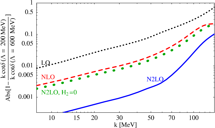
Figure 1: Double-logarithmic error plot for the ${}^{2}\mathrm{S}_{\frac{1}{2}}$ wave of $\mathrm{Nd}$ scattering in EFT($\not{\pi}$); cf. Refs. Bedaque:2002yg ; improve3body . Black dotted line: LO; red dashed: NLO; blue solid: N²LO with $H_{2}\neq 0$; green dotted: N²LO with $H_{2}\equiv 0$.

More informative is a look at the slopes in $\ln k$. Lines at different orders are near-parallel for small $k$ because there are additional natural low-energy scales $p_{\text{typ}}$, namely the binding momenta of the deuteron ($\gamma_{t}\approx 45\;\mathrm{MeV}$) and of the virtual singlet-S state ($\gamma_{s}\approx-8\;\mathrm{MeV}$). For $k\lesssim\gamma_{t,s}$, eqs. (5) and (10) are not very sensitive to $k$, so all slopes should indeed be small and near-identical. However, in the “window of opportunity” $k\gg\gamma_{t,s}$ (but of course still $k\ll\overline{\Lambda}_{\not{\pi}}$, so that the EFT converges), they converge towards one region. According to the discussion below eq. (10), slopes in that window are at order $Q^{n}$ given by $n+1-\eta$, with $\eta\leq n_{0}$ determined by the LO-dependence on $k$.

Indeed, the fits of $n$ to the nearly straight lines in the momentum range between $70\;\mathrm{MeV}>\gamma_{t,s}$ and $100$-to-$130\;\mathrm{MeV}\lesssim\overline{\Lambda}_{\not{\pi}}$ compare well to the PC prediction when $H_{2}$ is added at N²LO improve3body :

slope LO NLO N²LO N²LO without $$H_{2}$$

slope fit [sic!]

prediction not renormalised

(11)

The asterisk ^∗ serves as reminder that in the $3\mathrm{N}$ system, $k\cot\delta\sim Q^{2}$ ($n_{0}=2$) from eq. (3), but the observed LO slope at large $k$ is $(n=n_{0}=2)+1-\eta\stackrel{{\scriptstyle!}}{{\approx}}1.9$, forcing $\eta=1$ as input into the following predictions.

Without $H_{2}$ at N²LO, the slope does not improve from NLO. This is a clear signal that the PC is inconsistent without a momentum-dependent $3\mathrm{N}$ interaction at N²LO: Its assumptions do not bear out in the functional behaviour of this observable on $k$. On the other hand, when $H_{2}$ is included, the slope is markedly steeper than at NLO. The general agreement between predicted and fitted slope is astounding, and actually quite stable against variation of the fit range or of the two cutoffs $\Lambda_{1}$ and $\Lambda_{2}$. Only the LO numbers are somewhat sensitive, and only to the upper limit improve3body .

It may appear somewhat surprising that the slope increases by two units from NLO to N²LO when one includes $H_{2}$. One would have expected the change from each order to the next to be by only one unit. This may however stem from the “partially resummed formalism” used at that time, which resums some higher-order contributions. It may be worth revisiting this issue with J. Vanasse’s method to determine higher-order corrections in “strict perturbation” Vanasse:2013sda ; see also the extended note 4.1.0.12. But we will see in the notes 4.1.0.2 on “Assumptions of the Expansion” that a fitted slope which is larger than predicted does not invalidate the power counting – the converse does.

Finally, the figure provides a rough value of $\overline{\Lambda}_{\not{\pi}}\approx[120\dots 150]\;\mathrm{MeV}$ as the region where the fitted lines of different orders coalesce. This is not in disagreement with the breakdown scale expected of EFT($\not{\pi}$).

For completeness, fig. 2 provides a plot of $|k\cot\delta(\Lambda=900\;\mathrm{MeV})|$ ($k\cot\delta$ is complex above the $\mathrm{Nd}$ breakup, $k_{\mathrm{break}}\approx 52\;\mathrm{MeV}$). It shows that corrections from LO to NLO, and further on to N²LO, are indeed parametrically small up to $k\lesssim 140\;\mathrm{MeV}$. This provides information on the magnitude of each contribution, while the error plot of fig. 1 provides information on the magnitude of the variation of each contribution with $\Lambda$. The extracted breakdown scale of both agrees, as is to be expected.

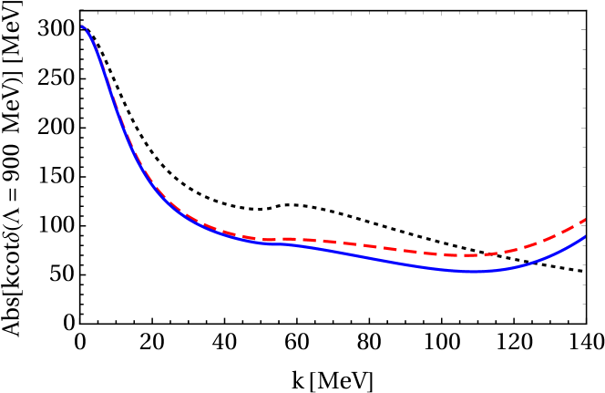
Figure 2: The magnitude of $k\cot\delta$ at cutoff $\Lambda=900\;\mathrm{MeV}$ in the ${}^{2}\mathrm{S}_{\frac{1}{2}}$ wave of $\mathrm{Nd}$ scattering in EFT($\not{\pi}$); cf. Refs. Bedaque:2002yg ; improve3body . Notation as in fig. 1.

4 Notes of Note

With this example in mind, we conclude by considering assumptions, strengths, extensions, features, caveats and limitations of such an analysis to assess the consistency of a PC proposal, grouped by three topics: comments directly relevant to the test; notes about the choice of observables, and concluding remarks. With in each topic, arguments progress from general to specific.

4.1 Matters of Principle

Let us first discuss more details about the fundamental assumptions, consequences and limitations of the procedure.

4.1.0.1 Extending the Expansion

In its original formulation, eq. (5) may at first glance insinuate that each order contains integer powers of the expansion parameter $Q$. However, the order $n$ is not necessarily an integer, and the first omitted order is not always $Q^{n+1}$, but more generally $Q^{n+\beta}$, $\mathrm{Re}[\beta]>0$. For example, some $\chi$EFT $\mathrm{NN}$ proposals in table 1 proceed in half-integer steps. To replace $n+1\to n+\beta$ in eqs. (4), (5), (10), (7) – and indeed throughout – is straightforward. In EFT($\not{\pi}$), the slope-fit in eq. (11) endorses that the $3\mathrm{N}$ PC proceeds in integer steps. Including non-analytic dependencies of the residuals on $k$ or $p_{\text{typ}}$ is also straightforward. For the remainder of the presentation, all such replacements are implied, but we stick to the integer case for convenience. One might also recall that arbitrarily small steps $\beta\to 0$ are not helpful unless the expansion parameter is extremely small. In that case, $\lim_{\beta\to 0}Q^{\beta}=1$ for fixed $Q$ implies that there is no ordering of terms in the series by relative size.

4.1.0.2 Assumptions of the Expansion

It is also appropriate to highlight and reiterate a few key premises. The assumptions on the residual $\mathcal{C}_{n}$ are endorsed if order $n$ and breakdown scale $\overline{\Lambda}_{\text{EFT}}$ follow indeed the functional form of eqs. (5) or its variants (10) and (7). Naïve Dimensional Analysis sets the magnitude of $\mathcal{C}_{n}$ to the scale of its running NDA ; NDA2 . Its cutoff-dependence and other effects are eventually absorbed into higher-order LECs, i.e. the cutoff dependence of observables should generically decrease order-by-order – even when no new fit parameters/LECs are encountered (see also below).

We can actually be somewhat more specific about the condition that the variation of the residual $\mathcal{C}_{n}$ with respect to $\Lambda$ should be larger than that for other parameters. Since $k,p_{\text{typ}}\ll\Lambda_{1},\Lambda_{2}$, the numerator on the left-hand side of eq. (5) can be expanded as

$$\begin{split}\mathcal{C}_{n}&(\Lambda_{1};k,p_{\text{typ}},\overline{\Lambda}_{\text{EFT}})-\mathcal{C}_{n}(\Lambda_{2};k,p_{\text{typ}},\overline{\Lambda}_{\text{EFT}})\\ &=c_{0}(\Lambda_{1},\Lambda_{2};\overline{\Lambda}_{\text{EFT}})+c_{1}(\Lambda_{1},\Lambda_{2};\overline{\Lambda}_{\text{EFT}})\;\frac{k,p_{\text{typ}}}{\Lambda_{1},\Lambda_{2}}+\dots\end{split}$$ (12)

If the first term dominates, then the dependence of eq. (5) on $k$ and $p_{\text{typ}}$ is indeed indicative of the order $Q^{n+1}$. If subsequent terms dominate, the exponent of eq. (5) may be larger than $n+1$ – but never smaller. Likewise, the slope of eq. (10) in the “window of opportunity” may be larger than $n+1-\eta$ (with $\eta\leq n_{0}$) – but never smaller.

4.1.0.3 Necessary but Not Sufficient

This last argument shows that an exponent smaller than $n+1$ conclusively demonstrates failure of the PC to be consistent. However, the criterion is necessary rather than sufficient: Exponents $\geq n+1$ (slopes $\geq n+1-\eta$ in the “window of opportunity”) are proof neither of failure, nor of success. Indeed, a PC may be inconsistent but the coefficient of the terms with exponent $<n+1$ may be anomalously small, leading to a “false negative”: The test does not reveal a problem, but the power counting is still inconsistent. Only understanding the limitations of the test allows one to avoid the danger of interpreting this as a “successful pass”.

4.1.0.4 Estimating the Expansion Parameter

As elaborated above, the test provides a direct prescription to find $\overline{\Lambda}_{\text{EFT}}$, and thus an estimate of the momentum-dependent expansion parameter $Q=\frac{k,p_{\text{typ}}}{\overline{\Lambda}_{\text{EFT}}}$ as a function of $k$. But it also allows for another practical way to assess $Q$: vary both cutoffs $\Lambda_{1}$ and $\Lambda_{2}$ over a wide range. Ratios between different orders estimate $Q(k,p_{\text{typ}})$, and hence residual theoretical uncertainties as a function of $k$. This is of course only one of several ways to assess $Q(k)$; within reason, the least optimistic and hence most conservative of several methods should be picked. For example, Ref. Griesshammer:2011md combined this with the convergence pattern of the EFT series Furnstahl:2015rha .

4.1.0.5 Choice of Expansion Parameter

In sect. 3, $k$ is varied while the other scales $p_{\text{typ}}$ are fixed, but any combination of the low-energy scales may serve as variable(s). For example, scanning in the pion mass at fixed $k\ll m_{\pi}$ may elucidate the $m_{\pi}$-dependence of some couplings. Recall that the chiral limit $m_{\pi}\to 0$ is of obvious importance in $\chi$EFT since its formal starting point is chiral symmetry. This was indeed explored in Ref. Beane:2001bc to demonstrate the inconsistency of Weinberg’s pragmatic proposal. It can also be of particular relevance to extrapolating lattice computations at non-physical pion masses. Likewise, varying the anomalous scales $\gamma_{t,s}$ may reveal information about how the EFT approaches the unitarity limit $\gamma_{t,s}\to 0$, whose importance for nuclear systems recently has been emphasised; see e.g. Kievsky:2015dtk ; Konig:2016utl ; Konig:2016iny ; Kolck:2017zzf ; Kievsky:2018xsl ; vanKolck:2019qea ; Konig:2019xxk . Here, I will continue to concentrate on variations with $k$, but most issues transfer straightforwardly to other variations.

4.1.0.6 Window of Opportunity

As stressed around eq. (5), one can read off logarithmic slopes most easily in the range $p_{\text{typ}}\ll k\ll\overline{\Lambda}_{\text{EFT}}$. In the EFT($\not{\pi}$) example above, that “window of opportunity” is narrow but appears to suffice: $\overline{\Lambda}_{\not{\pi}}/(p_{\text{typ}}\sim\gamma_{t,s})\lesssim 3$. In $\chi$EFT with dynamical $\Delta(1232)$ degrees of freedom, one would expect a wider range: $\overline{\Lambda}_{\chi}/(p_{\text{typ}}\sim m_{\pi})\gtrsim 4$. Still, the one-pion exchange scale of $\mathrm{NN}$ scattering, $\Lambda_{\mathrm{NN}}\approx 300\;\mathrm{MeV}$, which was mentioned in the Introduction, complicates the situation Kaplan:1998we ; Barford:2002je . If it is a low scale, $m_{\pi}<\Lambda_{\mathrm{NN}}\stackrel{{\scriptstyle?}}{{\ll}}\overline{\Lambda}_{\chi}$, the window of opportunity could possibly be halved to $\overline{\Lambda}_{\chi}/(p_{\text{typ}}\sim m_{\pi},\Lambda_{\mathrm{NN}})\approx 2$. In $\chi$EFT without explicit $\Delta(1232)$, $\Lambda_{\mathrm{NN}}$ is comparable to $\overline{\Lambda}_{\chi}(\not{\Delta})\approx 300\;\mathrm{MeV}$, therefore counts as a high scale, and one finds again a window of size $\overline{\Lambda}_{\chi}(\not{\Delta})/(p_{\text{typ}}\sim m_{\pi})\approx 2$. Only further, practical investigation can elucidate how big the window actually is in either EFT.

One may of course also fit the variables $n$ and $\overline{\Lambda}_{\text{EFT}}$ in eq. (5) to the numerical results below that window, but then one needs to specify the scales $p_{\text{typ}}$ and determine their contributions relative to $k$. This could be achieved by independently varying $p_{\text{typ}}$; see note 4.1.0.5 above. Alternatively, one can employ another trick discussed now.

4.1.0.7 Extending the Window of Opportunity

In the physically accessible world, the size of that window is prescribed because the scales $p_{\text{typ}}\sim m_{\pi},\gamma_{t,s},\dots$ have fixed values. We can however not only explore functional dependencies via variations of $p_{\text{typ}}$ directly as in 4.1.0.5; we can simply extend the window in which the slope of $k$ can be extracted by decreasing the scales $p_{\text{typ}}$. While data is available only at the physical point, an EFT power counting must remain formally consistent when its underlying qualitative assumptions are still valid. In $\chi$EFT, that is the interpretation of the pion as quasi-Goldstone boson of chiral symmetry ($m_{\pi}\ll\overline{\Lambda}_{\chi}$), and the existence of anomalously shallow binding scales in the $\mathrm{NN}$ system ($\gamma_{t,s}\ll m_{\pi}$), which in turn is related to the importance of the unitarity limit Kievsky:2015dtk ; Konig:2016utl ; Konig:2016iny ; Kolck:2017zzf ; Kievsky:2018xsl ; vanKolck:2019qea ; Konig:2019xxk . These assumptions do not depend on the particular values of $m_{\pi}$ or $\gamma_{t,s}$ off the physical point, so there is no need to explore how the parameters $\gamma_{t,s}$ correlate with $m_{\pi}$; that dependence was first studied in refs. Beane:2002xf ; Epelbaum:2002gb . Rather, one constructs multiverses with different pion masses and $\gamma_{t,s}$, only for the purpose of disentangling the multi-variate dependencies in eq. (5) and enlarging the window of opportunity in which a slope in $k$ should emerge.

4.1.0.8 Choice of Regulator

Residual cutoff dependence emerges naturally in numerical computations. This test uses it as a tool to check consistency, but how crucial are details of the regularisation procedure? The example in sect. 3 used a “hard” cutoff, but $\overline{\Lambda}_{\text{EFT}}$ and the exponent $n$ do not depend on a specific regulator. If the theory can be renormalised exactly, all residual regulator dependence disappears by dimensional transmutation; cf. (7). It may well be that the test is most decisive for regulators which are usually disfavoured because they show significant cutoff artefacts (but in which the residuals $\mathcal{C}_{n}$ are of course still of natural size).

4.1.0.9 Choice of Cutoffs

As just established, the functional dependencies of eqs. (5) and (7) on $n$ and $\overline{\Lambda}_{\text{EFT}}$ do not depend on $\Lambda_{1}$ and $\Lambda_{2}$. While any two cutoffs $\Lambda_{1},\Lambda_{2}\gtrsim\overline{\Lambda}_{\text{EFT}}$ will do in principle, small leverage may however lead to numerical artefacts. The larger $\Lambda_{2}-\Lambda_{1}$, the clearer the signal should be. For our example, fig. 3 shows that an upper cutoff of $900\;\mathrm{MeV}$ instead of $600\;\mathrm{MeV}$ leads indeed to different curves but very similar slopes, including for the N²LO result at $H_{2}=0$. Infinities, zeroes and oscillations of $\mathcal{O}$ with $k$ for any pair $\Lambda_{1},\Lambda_{2}$ can lead to problems (see note 4.2.0.4) which are readily avoided by choosing a cutoff pair such that $\mathcal{O}(\Lambda_{1})-\mathcal{O}(\Lambda_{2})>0$ for all $k$. Even when one does not choose to take one of the cutoffs to infinity, a reasonable range of allowed cutoffs exists. If $\Lambda_{1}\approx\Lambda_{2}$, one may of course directly consider the numerical derivative of eq. (7) – over a range of cutoffs. [To reiterate: exact cutoff independence $\mathcal{O}(\Lambda_{1})\equiv\mathcal{O}(\Lambda_{2})$ for any cutoff pair is not considered.]

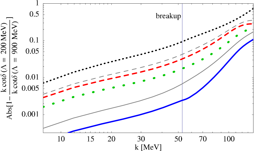
Figure 3: Thick coloured lines: Z-parametrisation of the $\mathrm{NN}$ amplitude as in fig. 1, but for $\Lambda_{1}=900\;\mathrm{MeV}$, not $600\;\mathrm{MeV}$; thin gray lines: Bethe’s Effective Range Parametrisation, whose LO is identical to that of Z-parametrisation; from Ref. improve3body . The N²LO result for $H_{2}=0$ in Z-parametrisation is included as in fig. 1 (thick green dots). This provides an example that different choices for the cutoff $\Lambda_{1}$ lead to different curves but similar slopes (compare the thick coloured lines to fig. 1), and that this holds also when different parametrisations are used (gray vs. coloured lines). Overall notation as in fig. 1.

4.1.0.10 Decreasing Cutoff Dependence

Equation (5) is a variant of the Renormalisation Group evolution of $\mathcal{O}$, eq. (7), which in turn quantifies the fundamental EFT tenet that observables must become order-by-order less sensitive to loop contributions beyond $\overline{\Lambda}_{\text{EFT}}$, the range of applicability. Cutoff dependence in observables should therefore generically decrease from order to order, irrespective whether or not LECs are fitted. This does not apply to the $\mathcal{C}_{n}$ themselves, but it does apply to the entire left-hand side of eq. (5). Refitting LECs may of course help to absorb some cutoff dependence. Indeed, no new LECs enter at NLO in the example above ($H_{0}$ is just refitted), and the cutoff dependence decreases from LO to NLO. While it is conceivable that the residual $\mathcal{C}_{n}$ is sometimes somewhat larger than Naïve Dimensional Analysis predicts, it should apply “most of the time”, statistically speaking and after appropriate Bayesian priors have been declared – see the comments below eq. (4).

Still, a specific regulator form may produce a very small residual cutoff dependence at one order but a significantly larger one at a subsequent order, $\mathcal{C}_{n}(\Lambda_{1})-\mathcal{C}_{n}(\Lambda_{2})<\mathcal{C}_{n+1}(\Lambda_{1})-\mathcal{C}_{n+1}(\Lambda_{2})$ for some $n$. This may for example occur if the regulator produces only corrections with even powers of $\Lambda$ and the numerics preserves this symmetry at least approximately (e.g. because $\Lambda_{1}\approx\Lambda_{2}$, allowing for a perturbative expansion). If this overwhelms the expansion in $Q$, $\mathcal{O}$ may indeed systematically become more dependent on $\Lambda$ between some orders, but not between all. Nonetheless, one should not just see some qualitatively improved cutoff dependence with increasing order, but one must see the quantitatively predicted slopes emerge for many orders: that they must be $\geq n+1-\eta$ at N${}^{n-n_{0}}$LO, provides a rigorous lower bound; see eqs. (10) and (12).

4.1.0.11 Constructing a PC by Trial-and-Error

This last point provides an opportunity. If the cutoff dependence of a given observable does not decrease consistently between subsequent orders, caution may be advisable. For example, $\Lambda$-dependence may increase from one order to the next, but then decrease markedly when another full order with a new LEC is included. This could signal that this LEC cures cutoff dependence already at a lower order – and hence that the PC is inconsistent. One should then study the convergence pattern as the LEC is promoted to a lower order such that the cutoff dependence decreases always between subsequent orders. This may help to construct a consistent PC by trial-and-error and iteration. Remember also that after a LEC starts contributing at a certain order, it is re-adjusted at each subsequent order to absorb both cutoff effects and still match its determining datum.

4.1.0.12 Calculating Higher Orders

Traditionally, observables beyond LO have been found by “partially resumming” contributions, i.e. the power-counted potential is iterated like in Weinberg’s original suggestion. Since corrections to the LO potential are defined as parametrically small, they can be included in “strict perturbation”. This avoids two recurring problems. First, spurious deeply bound states can be generated by iteration. This usually becomes the more problematic, the higher the order or the larger the cutoff $\Lambda$ improve3body ; Vanasse:2013sda . Second, partial resummation often softens the (unphysical) ultraviolet behaviour of the amplitude, so that fewer LECs appear to be necessary to cure residual cutoff dependence. A striking example of this is found yet again in the $3\mathrm{N}$ system of EFT($\not{\pi}$) Gabbiani:2001yh . There, a careless resummation of effective-range contributions at LO appears to eliminate the need for the three-nucleon interaction which is central for the Efimov effect. That also happens to lead to results which are not supported by data. A “strictly perturbative” approach may provide clearer signals for the PC test than a partially-resummed one.

4.2 Picking Observables

The comments in this section discuss that not all observables are equally suited for clear results of the proposed test, and provide criteria to identify those that are more likely to be.

4.2.0.1 Isolating Dynamical Effects

While any observable could be chosen, those which are free from kinematic or other constraints (e.g. from symmetries) are preferred. Consider the scattering amplitude $\mathcal{A}_{l}$ in the $l$th partial wave (for simplicity, assume no mixing). Since it is complex, one could choose $\mathcal{O}=|\mathcal{A}_{l}|$. However, unitarity relates $\mathcal{A}_{l}=1/(k\cot\delta_{l}-\mathrm{i}k)$ to the phase shift $\delta_{l}$. This constraint dominates when $\delta_{l}$ is between about $\pi/4$ and $3\pi/4$ – which affects much of the $\mathrm{NN}$ S-wave phase shifts. Even outside this interval, the additional contribution to eqs. (5) and (10) is not sensitive to dynamics. In addition, analyticity dictates that phase shifts approach zero like $k^{2l+1}$ for $k\to 0$ in the $l$th partial wave. Since both numerator and denominator in eq. (5) are then zero, $\mathcal{O}=\delta_{l}$ is dominated by numerical uncertainties as $k\to 0$. This may not be a problem if the region in which the slopes are determined is far away, but only a closer inspection could tell if that holds. Likewise, it may be prudent to eliminate phase-space factors of effects from cuts in decay constants, production cross sections, etc, to arrive at “smooth” functions to analyse.

A sensible choice for single-channel scattering appears thus to be $\mathcal{O}=k^{2l+1}\cot\delta_{l}$: It is only constrained to be real below the first inelasticity, and imaginary parts are usually small above it. One can then choose to consider its magnitude, or real and imaginary parts separately Dai:2017ont . Indeed, the S-wave example above kept track of the imaginary part by plotting

$$\left|1-\frac{k\cot\delta_{0}(\Lambda_{2})}{k\cot\delta_{0}(\Lambda_{1})}\right|\;\;.$$ (13)

While factors of $k$ formally cancel, one should remember that the numerics of calculating $\mathcal{A}$ (i.e. $k\cot\delta_{0}$) is more benign when the powers of $k$ are kept.

In the EFT($\not{\pi}$) example above, examining

$$1-\frac{|k\cot\delta_{0}(\Lambda_{2})|}{|k\cot\delta_{0}(\Lambda_{1})|}$$ (14)

is disfavoured. In that form, there appears for each pair of cutoff values a momentum $k_{0}$ in a range around $100\;\mathrm{MeV}$ inside the “window of opportunity” where the results of both cutoffs appear to agree (“accidental zero”; see also note 4.2.0.5 below).

4.2.0.2 Partial-Wave Mixing

In the $\mathrm{NN}$ system, two partial waves with total angular momentum $J$ mix. The corresponding unconstrained observables in the Stapp-Ypsilanti-Metropolis (SYM or “nuclear-bar”) parametrisation are

$$k^{2\pm 1-2J}\bar{\delta}_{J\pm 1}\;\;\mbox{ and }\;\;k^{-(2J+1)}\bar{\epsilon}_{J}\;\;.$$ (15)

In the Blatt-Biedenharn parametrisation, the same rules apply for the eigenphases, but $k^{-2}\epsilon_{J}$ is the unconstrained variable for the mixing angle; see e.g. deSwart:1995ui . These choices do not suffer from unitarity constraints (except for being real below the first inelasticity) and can be used directly.

4.2.0.3 Dependence on Parameter Input

The test’s goal is to resort minimally to empirical data, ideally only relying on the existence of anomalously shallow scales in a theory whose LO is non-perturbative, but not on their exact values. Instead, the goal is to focus on consistency of the EFT. To which degree can one achieve that? First, consider processes in which $\mathcal{O}(k)$ is a parameter-free prediction, i.e. its LECs are all known from some other process(es). To what extent does the procedure depend on that choice? In the example, the two-nucleon interactions were determined to match the Z-parametrisation of $\mathrm{NN}$-scattering (by fitting to the pole position and residue of the scattering amplitude) Phillips:1999hh . Figure 3 shows that results with Bethe’s Effective-Range Parametrisation have a markedly different rate of convergence, but the extracted slopes and $\overline{\Lambda}_{\not{\pi}}$ agree very well improve3body . Note that LO is identical in both parametrisations.

4.2.0.4 Accidental Zeroes and Infinities

Some observables may however show additional structures which should be avoided. For example, the ${}^{3}\mathrm{P}_{0}$ phase shift in $\mathrm{NN}$ scattering is zero at a lab energy of about $150\;\mathrm{MeV}$, so that the relative deviation of $\mathcal{O}=\delta_{l}$ in eq. (5) diverges. Likewise, $\mathcal{O}=k^{2l+1}\cot\delta_{l}$ diverges (approaches zero) at $\delta_{l}=0$ ($\pi/2$), e.g. in the ${}^{1}\mathrm{S}_{0}$ wave at $k\approx 370\;\mathrm{MeV}$ and ${}^{3}\mathrm{S}_{1}$ wave at $k\approx 90\;\mathrm{MeV}$ and $400\;\mathrm{MeV}$ Epelbaum:2014efa . As the qualitative plot in fig. 4 shows, the corresponding spikes may make it more difficult to determine slopes.

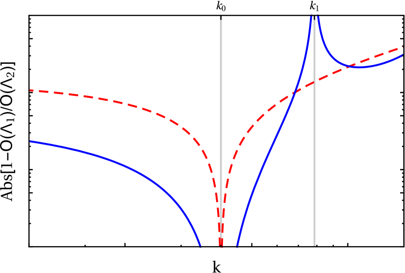
Figure 4: Qualitative example of the impact of zeroes in $\mathcal{O}(\Lambda_{2})-\mathcal{O}(\Lambda_{1})$ (exact reproduction of datum at $k_{0}$), and in $\mathcal{O}(\Lambda)$ (“accidental zero” of $\mathcal{O}(\Lambda_{1})$ at $k_{1}$). Red dashed line: $n=1$; blue solid: $n=2$.

4.2.0.5 Fitting to a Point

Such a “zero” in eq. (5) is actually induced intentionally when the observable contains a LEC that is determined in the channel in which one tests the PC. If the observable is tuned to exactly reproduce a certain value at some point $(k_{0},p_{\text{typ}})$, then $\mathcal{O}(k_{0};\Lambda_{1})-\mathcal{O}(k_{0};\Lambda_{2})=0$ – with all the problems mentioned just now. Obviously, one should choose the fit point to be outside the “window of opportunity”. In the example of sect. 3, the strength of the $3\mathrm{N}$ interaction $H_{0}$ without derivatives was fixed at each order to the $\mathrm{Nd}$ scattering length, i.e. using $k=0$ as fit point. That is far away from the “window of opportunity”. At N²LO, the momentum-dependent $3\mathrm{N}$ interaction $H_{2}$ was in addition determined from the triton binding energy $B_{3}=8.48\;\mathrm{MeV}$, i.e. the pole in the amplitude is fixed to $k_{0}=\sqrt{-4MB_{3}/3}\approx 100\;\mathrm{i}\;\mathrm{MeV}$. If one chooses this fit point for $H_{0}$ at LO and NLO, instead of $k_{0}=0$, the pattern of the slopes is wiped out; see fig. 5. It appears that fitting only at $k_{0}$ introduces a new low-energy scale $p_{\text{typ}}$ and leaves no window $\overline{\Lambda}_{\not{\pi}}\gg k\gg|k_{0}|\approx 100\;\mathrm{MeV}$, while the N²LO fit at both $k=0$ and $k_{0}$ does not suffer this limitation.

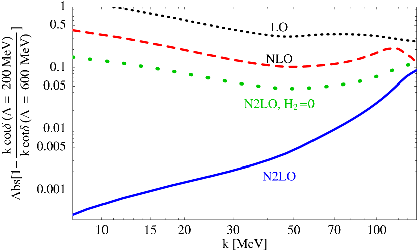
Figure 5: Test when the leading $3\mathrm{N}$ interaction is determined not by the $\mathrm{Nd}$ scattering length as in fig. 1, but by the position of the triton pole. The N²LO fit uses again the $\mathrm{Nd}$ scattering length and triton binding energy.

4.2.0.6 Fitting in a Region

The issue is less transparent when the LEC is not determined by exactly reproducing some data, but by fitting over a whole region in $k$. That is the typical case in $\mathrm{NN}$ scattering (see e.g. Ref. Epelbaum:2014efa ), and in $\overline{\mathrm{N}}\mathrm{N}$ scattering Dai:2017ont . The deviation of the fitted result from data is more regular at any given cutoff $\Lambda$ than when it is exactly zero at $k_{0}$. A pronounced spike is therefore replaced by a more uniformly, but also more stealthily, constrained behaviour inside the fit region. The comparison between two cutoffs in eqs. (5) and (10) is thus also more uniform as a function of $k$. Since cutoff variations can now be balanced by adjusting LECs, the coefficients $\mathcal{C}_{n}$ are artificially small in that régime. One still expects the cutoff dependence to decrease order-by-order, but the characteristic slopes are harder to see since the observable is constrained by the fit. Just like in the neighbourhood of a fit point, an observable will first have to shed the fit constraints outside the fit region for pronounced slopes to emerge.

Such a fit region must of course be inside the applicability range of the EFT. Traditional fits do not take into account that the systematic uncertainties of an EFT increase with $k$, but assign a $k$-independent uncertainty weight. Equation (4) suggests that this is justified for $k\lesssim p_{\text{typ}}$ since the error varies only mildly. In that case, one can speculate that the impact on the slopes at higher $k$ is not too big. This limits a reasonable fit region to $k\lesssim\gamma_{t,s}$ in EFT($\not{\pi}$); and to $k\lesssim m_{\pi}$ in $\chi$EFT. In addition, one expects clearer signals if the same fit region is used at each order. It is difficult to see how slopes can clearly be identified when the fit region extends far towards $\overline{\Lambda}_{\text{EFT}}$. Practical considerations, like insufficient or low-quality data at low momenta, may well override this choice. But there is a way around, as discussed now.

4.2.0.7 Fitting to Pseudo-Data

As a recourse and in order to assess the impact of a fit region on the slopes, one may create an artificial, “exact datum” $\mathcal{O}_{0}(k_{0})$ at very low $k\to 0$ which agrees with low-energy data (e.g. a scattering length, effective range, etc); and then assess the dependence of the slope on reasonable variations of $\mathcal{O}_{0}(k_{0})$. The goal is then not to find good agreement with actual data at higher energies, but to test the convergence pattern. An EFT will not become inconsistent just because some particular datum is shifted by some small amount, or because the error bar on a datum is substantially reduced. For example, the power-counting for $\mathrm{NN}$ amplitudes in eq. (2) only uses that there is a shallow real or virtual bound state, not its exact location.

4.2.0.8 Summary: Choice of Observable

Ideal candidates for $\mathcal{O}$ are positive-definite observables which are not subject to unitarity and other constraints, and which are nonzero and finite over a wide range in $k$ and $\Lambda$, including the régime $k\gtrsim p_{\text{typ}}$ where one hopes to determine the slope. EFT parameters/LECs should be determined at very low $k$. A good signal may need some creativity. The choices $\mathcal{O}=k^{2l+1}\cot\delta_{l}$, $k^{2\pm 1-2J}\bar{\delta}_{J\pm 1}$ and $k^{-(2J+1)}\bar{\epsilon}_{J}$, with Effective-Range parameters determining unknowns, appear suitable in most scattering cases.

4.3 Miscellaneous Notes

Finally, the following notes wrap up a variety of issues.

4.3.0.1 Consistency Assessment vs. “Lepage Plots” and Other Data-Driven Approaches

To put this test into a broader context, one should note that double-logarithmic convergence plots are not unfamiliar. Lepage compared to data in order to quantify how accurately the EFT reproduces experimental information Lepage:1997cs . This triggered a series of influential studies of differences between approximations and “exact results” in toy-models, see e.g. Steele:1998un ; Steele:1998zc ; Kaplan:1999qa . More recently, Birse and collaborators perused similar techniques, after removing the strong influence of long-range Physics (One- and Two-Pion Exchange) from empirical phase shifts in a modified Effective Range Expansion. This allows a more detailed study of the residual short-distance interactions under the assumption that long-distance Physics is generally agreed upon to be understood sufficiently well Birse:2007sx ; Birse:2010jr ; Ipson:2010ah . As table 1 shows, that is true for one-pion exchange, but not for two-pion exchange. Both of these alternative approaches rely on a high-quality, data-based partial wave analysis.

The test advocated here emphasises somewhat different aspects. It tries to minimise dependence on data, depending only on empirical input which is mostly qualitative: the existence of anomalously small scales, and of some low-momentum window in which a few data can be used to determine LECs. It then aims to answer complementing questions: Does the output match the assumptions? Is the theory consistent, and consistently renormalised in both its long- and short-range aspects? Recall that an EFT may converge by itself, but not to data, if some dynamical degrees of freedom are incorrect or missing. For example, a $\chi$EFT without dynamical $\Delta(1232)$ at $k\approx 300\;\mathrm{MeV}$ cannot reproduce Delta resonance properties – but it may well be consistent.

In other words, an EFT may be consistent by itself, but not consistent with Nature.

4.3.0.2 Insensitivity to Some LECs

This procedure can only help determine if a LEC is correctly accounted for when it is needed to absorb residual cutoff dependence. Equation (7) then determines its running, and its initial condition is fixed by some input, for example data or results of a more fundamental theory. Some LECs do however start contributing just because of their natural size, and not to renormalise that order. For example, the magnetic moment of the nucleon enters the one-baryon Lagrangean of $\chi$EFT at NLO, albeit it is not needed to renormalise loops. Similarly, the contribution of a LEC to a particular observable may be unnaturally small (or even zero).

4.3.0.3 Numerics

The analysis can be numerically indecisive. We would trust results only if $n$ and $\overline{\Lambda}_{\text{EFT}}$ can be determined quite robustly in a reasonably wide range to cutoffs (and, possibly, cutoff forms), parameter sets and fit-windows. None of this provides, however, sufficient excuse not to report results.

4.3.0.4 Sampling Tests

Finding that the exponent at each order $Q^{n}$ is not smaller than $n+1-n_{0}$ is necessary but not sufficient for a consistent PC. We saw that fine-tuning, particular choices of regulator forms and observables, and anomalously small coefficients are some reasons which may hide signals of exponents $<n+1-n_{0}$ which violate the PC assumptions. If exponents are always $\geq n+1-n_{0}$ for a variety of independent observables, regulators etc., that may increase confidence in PC consistency – but cannot prove it. The same statement holds when the exponent $n+1-n_{0}$ is substituted by the slopes $n+1-\eta$ in the “window of opportunity”.

That is why this is a falsification test.

4.4 Outlook

Unnaturally small scales provide significant challenges to formulating a power-counting scheme in EFTs when analytic results cannot be obtained. This presentation advocated a quantitative and pragmatic test which can falsify a proposed scheme, and which may elucidate the power-counting issues which plague $\chi$EFT. It provides a necessary but not sufficient consistency criterion.

In its simplest and, for now, only tested variant, a “window of opportunity” is necessary, in which all low scales but one momentum scale $k$ can be neglected, but in which the EFT still converges, $k\ll\overline{\Lambda}_{\text{EFT}}$. This may be problematic in $\chi$EFT because it is not quite clear what role is played by $\Lambda_{\mathrm{NN}}\approx 300\;\mathrm{MeV}$, the strength-scale of the $\mathrm{NN}$ potential; see discussion in 4.1.0.6.

The $\chi$EFT power-counting proposals differ most starkly in the attractive triplet partial waves of $\mathrm{NN}$ scattering since they reflect different philosophies on how to treat the non-selfadjoint, attractive $1/r^{3}$ potential at short distances which appears at leading order; see table 1. It would therefore be interesting to see this test applied to the ${}^{3}\mathrm{P}_{0}$ wave and to the ${}^{3}\mathrm{P}_{2}$-${}^{3}\mathrm{F}_{2}$ system; and work is indeed under way Yang:2019hkn ; hgrieYang . In addition, one should explore whether one can merge the present approach with the work of Birse and collaborators Birse:2007sx ; Birse:2010jr ; Ipson:2010ah . As one referee pointed out, it may be possible to analyse quasi-data generated at different EFT orders using the modified Effective Range Expansion to more clearly isolate short-distance effects.

The test proposed here is not necessarily a silver bullet to endorse or reject a particular counting since its results may in the worst case be inconclusive. It is thus neither more nor less than one more arrow in the quiver to test EFTs. But that implies it is still worth a try.

Data Availability Statement

The preciously few data underlying this work are available in full upon request from the author.

References

- (1) The Editors, Editorial: Uncertainty Estimates, Phys. Rev. A83, 040001 (2011).
- (2) Enhancing the Interaction between Nuclear Experiment and Theory Through Information and Statistics, special issue J. Phys. G 42 number 3 (March 2015).
- (3) Further Enhancing the Interaction between Nuclear Experiment and Theory through Information and Statistics (ISNET 2.0), special issue J. Phys. G 46 number 10 (2019, publication ongoing).
- (4) G. P. Lepage, [nucl-th/9706029].
- (5) R. Landau, J. Páez and C. Bordeianu, A Survey of Computational Physics: Introductory Computational Science, Princeton University Press, 2008: chapter 2.3.
- (6) P. F. Bedaque, H. W. Grießhammer, G. Rupak and H.-W. Hammer, Nucl. Phys. A 714, 589 (2003) [nucl-th/0207034].
- (7) H. W. Grießhammer, Nucl. Phys. A 744, 192 (2004) [nucl-th/0404073].
-
(8)
H. W. Grießhammer, Introduction to Effective Field
Theories, National Nuclear Physics Summer School 2008,
Washington DC (USA); notes at home.gwu.edu/
hgrie/. - (9) H. W. Grießhammer, Summary: Systematising the System in Chiral Effective Field Theory, remarks at Nuclear Forces from Effective Field Theory, CEA/SPhN Saclay (France) 2013.
- (10) H. W. Grießhammer, Testing a Power Counting, remarks at Bound States and Resonances in Effective Field Theories and Lattice QCD Calculations, Benasque (Spain) 2014.
- (11) R. J. Furnstahl, D. R. Phillips and S. Wesolowski, J. Phys. G 42, 034028 (2015) [arXiv:1407.0657 [nucl-th]].
- (12) E. Epelbaum, H. Krebs and U. G. Meißner, Eur. Phys. J. A 51, 53 (2015) [arXiv:1412.0142 [nucl-th]].
- (13) L. Y. Dai, J. Haidenbauer and U. G. Meißner, JHEP 1707, 078 (2017) [arXiv:1702.02065 [nucl-th]].
- (14) H. W. Grießhammer, PoS CD 15, 104 (2016) [arXiv:1511.00490 [nucl-th]].
- (15) H.-W. Hammer, S. König and U. van Kolck, [arXiv:1906.12122 [nucl-th]].
- (16) A. Manohar and H. Georgi, Nucl. Phys. B 234, 189 (1984) [n.b. Acknowledgement].
- (17) H. Georgi and L. Randall, Nucl. Phys. B 276, 241 (1986).
- (18) S. Weinberg, Phys. Rev. Lett. 63, 2333 (1989).
- (19) H. Georgi, Phys. Lett. B 298, 187 (1993) [hep-ph/9207278].
- (20) H. W. Grießhammer, Nucl. Phys. A 760, 110 (2005) [nucl-th/0502039].
- (21) M. Beneke and V. A. Smirnov, Nucl. Phys. B 522, 321 (1998) [hep-ph/9711391].
- (22) H. W. Grießhammer, Phys. Rev. D 58, 094027 (1998) [hep-ph/9712467].
- (23) D. B. Kaplan, M. J. Savage and M. B. Wise, Phys. Lett. B 424, 390 (1998) [nucl-th/9801034].
- (24) D. B. Kaplan, M. J. Savage and M. B. Wise, Nucl. Phys. B 534, 329 (1998) [nucl-th/9802075].
- (25) S. Fleming, T. Mehen and I. W. Stewart, Nucl. Phys. A 677, 313 (2000) [nucl-th/9911001].
- (26) T. Barford and M. C. Birse, Phys. Rev. C 67, 064006 (2003) [arXiv:hep-ph/0206146 [hep-ph]].
- (27) P. F. Bedaque and U. van Kolck, Ann. Rev. Nucl. Part. Sci. 52, 339-396 (2002) [nucl-th/0203055].
- (28) L. Platter, Few Body Syst. 46, 139-171 (2009) [arXiv:0904.2227 [nucl-th]].
- (29) S. R. Beane, P. F. Bedaque, M. J. Savage and U. van Kolck, Nucl. Phys.A 700, 377 (2002) [nucl-th/0104030].
- (30) A. Nogga, R. G. E. Timmermans and U. van Kolck, Phys. Rev. C 72, 054006 (2005) [nucl-th/0506005].
- (31) U. van Kolck, this volume.
- (32) E. Epelbaum and U.-G. Meissner, Few Body Syst. 54, 2175 (2013) [nucl-th/0609037].
- (33) S. Weinberg, Nucl. Phys. B 363, 3 (1991).
- (34) M. C. Birse, Phys. Rev. C 74, 014003 (2006) [nucl-th/0507077].
- (35) M. C. Birse, PoS CD 09, 078 (2009) [arXiv:0909.4641 [nucl-th]].
- (36) M. P. Valderrama, Phys. Rev. C 83, 024003 (2011) [arXiv:0912.0699 [nucl-th]].
- (37) M. Pavon Valderrama, Phys. Rev. C 84, 064002 (2011) [arXiv:1108.0872 [nucl-th]].
- (38) M. Pavon Valderrama, [arXiv:1902.08172 [nucl-th]].
- (39) B. Long and C. J. Yang, Phys. Rev. C 85, 034002 (2012) [arXiv:1111.3993 [nucl-th]].
- (40) B. Long and C. J. Yang, Phys. Rev. C 86, 024001 (2012) [arXiv:1202.4053 [nucl-th]].
- (41) D. R. Phillips, PoS CD 12, 013 (2013) [arXiv:1302.5959 [nucl-th]].
- (42) U. van Kolck, Front. Phys., in press [arXiv:2003.06721 [nucl-th]].
- (43) D. B. Kaplan, M. J. Savage and M. B. Wise, Nucl. Phys. B 478, 629 (1996) [nucl-th/9605002].
- (44) S. R. Beane, D. B. Kaplan and A. Vuorinen, Phys. Rev. C 80, 011001 (2009) [arXiv:0812.3938 [nucl-th]].
- (45) E. Epelbaum and J. Gegelia, Eur. Phys. J. A 41, 341 (2009) [arXiv:0906.3822 [nucl-th]].
- (46) M. P. Valderrama, Int. J. Mod. Phys. E 25, 1641007 (2016) [arXiv:1604.01332 [nucl-th]].
- (47) U. van Kolck, Tower of Effective Field Theories: Status and Perspectives, workshop The Tower of Effective (Field) Theories and theEmergence of Nuclear Phenomena (EFT and Philosophy of Science) at CEA/SPhN Saclay, 17 January 2017.
- (48) G. ’t Hooft, NATO Sci. Ser. B 59, 135 (1980).
- (49) William of Occam (or Ockham) is generally credited, but the exact reference is not fully resolved. A commonly mentioned text appears to be Quaestiones et decisiones in quattuor libros Sententiarum Petri Lombardi ed. Lugd. (1495), i, dist. 27, qu. 2, K.
- (50) A. Einstein in R. W. Clark, Einstein: The Life and Times, William Morrow pub. (1973), chap. 14.
- (51) Anonymous, priv. comm.
- (52) E. Braaten and H.-W. Hammer, Phys. Rept. 428, 259 (2006) [cond-mat/0410417].
- (53) J. Schwinger, hectographed notes on nuclear physics, Harvard University 1947
- (54) G. F. Chew and M. L. Goldberger, Phys. Rev. 75, 1637 (1949)
- (55) F. C. Barker and R. E. Peierls, Phys. Rev. 75, 3122 (1949)
- (56) H. A. Bethe, Phys. Rev. 76, 38 (1949).
- (57) H. W. Grießhammer and M. R. Schindler, Eur. Phys. J. A 46, 73 (2010) [arXiv:1007.0734 [nucl-th]].
- (58) J. Vanasse, Phys. Rev. C 99, 054001 (2019) [arXiv:1809.10740 [nucl-th]].
- (59) H. W. Grießhammer, Nucl. Phys. A 760 (2005), 110 [nucl-th/0502039].
- (60) L. Platter and D. R. Phillips, Few Body Syst. 40, 35 (2006) [cond-mat/0604255].
- (61) C. Ji and D. R. Phillips, Few Body Syst. 54, 2317 (2013) [arXiv:1212.1845 [nucl-th]].
- (62) J. Vanasse, Phys. Rev. C 88, 044001 (2013) [arXiv:1305.0283 [nucl-th]].
- (63) H. W. Grießhammer, M. R. Schindler and R. P. Springer, Eur. Phys. J. A 48, 7 (2012) [arXiv:1109.5667 [nucl-th]].
- (64) R. J. Furnstahl, N. Klco, D. R. Phillips and S. Wesolowski, Phys. Rev. C 92, 024005 (2015) [arXiv:1506.01343 [nucl-th]].
- (65) A. Kievsky and M. Gattobigio, Few Body Syst. 57 (2016) 217 [arXiv:1511.09184 [nucl-th]].
- (66) S. König, H. W. Grießhammer, H. W. Hammer and U. van Kolck, Phys. Rev. Lett. 118, no. 20, 202501 (2017) [arXiv:1607.04623 [nucl-th]].
- (67) S. König, J. Phys. G 44, no. 6, 064007 (2017) [arXiv:1609.03163 [nucl-th]].
- (68) U. van Kolck, Few Body Syst. 58, no. 3, 112 (2017).
- (69) A. Kievsky, M. Viviani, D. Logoteta, I. Bombaci and L. Girlanda, Phys. Rev. Lett. 121, no. 7, 072701 (2018) [arXiv:1806.02636 [nucl-th]].
- (70) U. van Kolck, Nuovo Cim. C 42, no. 2-3-3, 52 (2019).
- (71) S. König, [arXiv:1910.12627 [nucl-th]].
- (72) S. R. Beane and M. J. Savage, Nucl. Phys. A 717, 91 (2003) [nucl-th/0208021].
- (73) E. Epelbaum, U. G. Meißner and W. Glöckle, Nucl. Phys. A 714, 535 (2003) [nucl-th/0207089].
- (74) F. Gabbiani, [nucl-th/0104088].
- (75) J. J. de Swart, C. P. F. Terheggen and V. G. J. Stoks, [nucl-th/9509032].
- (76) D. R. Phillips, G. Rupak and M. J. Savage, Phys. Lett. B 473, 209 (2000) [nucl-th/9908054].
- (77) J. V. Steele and R. J. Furnstahl, Nucl. Phys. A 637, 46 (1998) [nucl-th/9802069].
- (78) J. V. Steele and R. J. Furnstahl, Nucl. Phys. A 645, 439 (1999) [nucl-th/9808022].
- (79) D. B. Kaplan and J. V. Steele, Phys. Rev. C 60, 064002 (1999) [nucl-th/9905027].
- (80) M. C. Birse, Phys. Rev. C 76, 034002 (2007) [arXiv:0706.0984 [nucl-th]].
- (81) M. C. Birse, Eur. Phys. J. A 46, 231 (2010) [arXiv:1007.0540 [nucl-th]].
- (82) K. L. Ipson, K. Helmke and M. C. Birse, Phys. Rev. C 83, 017001 (2011) [arXiv:1009.0686 [nucl-th]].
- (83) C.-J. Yang, Eur. Phys. J. A 56, no. 3, 96 (2020) doi:10.1140/epja/s10050-020-00104-0 [arXiv:1905.12510 [nucl-th]].
- (84) H. W. Grießhammer and Ch.-J. Yang, in preparation.