Automated Configuration of Negotiation Strategies

Abstract.

Bidding and acceptance strategies have a substantial impact on the outcome of negotiations in scenarios with linear additive and nonlinear utility functions. Over the years, it has become clear that there is no single best strategy for all negotiation settings, yet many fixed strategies are still being developed. We envision a shift in the strategy design question from: What is a good strategy?, towards: What could be a good strategy? For this purpose, we developed a method leveraging automated algorithm configuration to find the best strategies for a specific set of negotiation settings. By empowering automated negotiating agents using automated algorithm configuration, we obtain a flexible negotiation agent that can be configured automatically for a rich space of opponents and negotiation scenarios.

To critically assess our approach, the agent was tested in an ANAC-like bilateral automated negotiation tournament setting against past competitors. We show that our automatically configured agent outperforms all other agents, with a 5.1% increase in negotiation payoff compared to the next-best agent. We note that without our agent in the tournament, the top-ranked agent wins by a margin of only 0.01%.

1. Introduction

As of the 1980s, researchers have tried to design algorithms (or software agents) that can assist or act on behalf of humans in negotiations. Early adopters in this field are Smith, Sycara, Robinson, Rosenschein and Klein Smith (1980); Sycara (1988); Sycara-Cyranski (1985); Robinson (1990); Rosenschein (1986); Klein and Lu (1989).

In 2010, the General Environment for Negotiation with Intelligent multi-purpose Usage Simulation Lin et al. (2014) (GENIUS) platform was created to provide a test-bed for evaluating new developments in the field of automated negotiation. Alongside, the Automated Negotiating Agents Competition Baarslag et al. (2012) (ANAC) competition series was organized to stimulate the development of negotiation algorithms in academia. Every year, ANAC poses a new challenge for contestants to cope with. Today, the combined effort of GENIUS and ANAC has resulted in a standardized test-bed with more than 100 negotiating agents and negotiation scenarios that are readily accessible for research on automated negotiation Baarslag et al. (2015).

The negotiators are generally hard-coded software agents, based on a strategy with fixed parameters that are tuned at design time to optimize its behavior. The difficulty lies not in developing a negotiator, but in winning the competition, as both the configuration space and the space of negotiation scenarios are large, and the competing agents change every year.

This makes manual configuration on larger sets of negotiation instances tedious, time-consuming and impractical. Furthermore, note that evaluating a single strategy on a large set of negotiation scenarios takes too much time to be practical.

To avoid these difficulties, agents have been configured on smaller sets Matos et al. (1998). Attempts were made to automate this process, for example using genetic programming Holland (1992), but again only on specific and simplified test sets. For instance, agents were only tested in one or two scenarios, or merely optimized against themselves Eymann (2001); Dworman et al. (1996). The resulting agents are highly specialized with unpredictable performance when negotiating outside of their comfort zone. No attempts have been reported at automating this configuration task on large-scale, broad sets of negotiation scenarios and opponent strategies.

In this work, we present a solution for the automated algorithm configuration problem for automated negotiation on large problem sets. We recreate a negotiation agent from literature Lau et al. (2006) that is configured manually, combine it with contemporary opponent learning techniques and create a configuration space of its strategic behavior. To automatically configure this conceptually rich and highly parametric design, we use Sequential Model-based optimization for general Algorithm Configuration Hutter et al. (2011) (SMAC), a general-purpose automated algorithm configuration procedure that has been used previously to optimize the performance of cutting-edge solvers for Boolean Satisfiability (SAT), Mixed Integer Programming (MIP) and other NP-hard problems. We note that here, we apply automated algorithm configuration for the first time to a multi-agent problem.

The aim of this work is to automatically configure a negotiation algorithm with no fixed or pre-defined strategy. This agent can be configured to perform well on a user-defined set of training problem instances, with little restrictions on the size of the instances or instance sets. To demonstrate its performance, we configure the agent in an attempt to win an ANAC-like bilateral tournament.

We show that we can win such a tournament with a comfortable margin of 5.1% in increased negotiation payoff compared to the number two. These margins are not observed in a tournament without our negotiation agent, where the winning strategy obtains a marginal improvement in negotiation payoff of 0.012%.

2. Related work

In this section, we discuss related work in the field of automated algorithm configuration, as well as some past applications in the research area of automated negotiation.

2.1. Automated algorithm configuration

In literature, automated algorithm configuration is also referred to as parameter tuning or hyperparameter optimization (in machine learning). It can be formally described as follows: given a parameterized algorithm $A$, a set of problem instances $I$ and a cost metric $c$, find parameter settings of $A$ that minimize $c$ on $I$ Hutter et al. (2011). The configuration problem occurs for example in solvers for MIP problems Hutter et al. (2010), neural networks, classification pipelines, and every other algorithm that contains performance-relevant parameters.

These configuration problems can be solved by basic approaches such as manual search, random search, and grid search, but over the years researchers developed more intelligent methods to obtain the best possible configuration for an algorithm. Two separate part within these methods can be identified: how new configurations are selected for evaluation and how a set of configurations is compared.

F-Race Birattari et al. (2010) races a set of configurations against each other on an incremental set of target instances and drops low performing configurations in the process. This saves computational budget, as not all configurations have to be tested on the full target instance set. The set of configurations to test can be selected either manually, as a grid search, or at random. Balaprakash et al. Balaprakash et al. (2007) extended upon F-Race by implementing it as a model-based search Zlochin et al. (2004), which iteratively models and samples the configuration space in search of promising candidate configurations.

ParamILS Hutter et al. (2009) does not use a model, but instead performs a local tree search operation to iteratively find better configurations. Like F-Race, ParamILS is capable of eliminating low performing configurations without evaluating them on the full set of instances.

Another popular method of algorithm configuring is GGA Ansótegui et al. (2009), which makes use of genetic programming to find configurations that perform well. This method does not model the configuration space and has no method to eliminate low performing configurations early.

The final method we want to mention is SMAC, which is an algorithm configuration method that uses a random forest model to predict promising configurations. It also includes an early elimination mechanism for promising configurations by comparing them with a dominant incumbent configuration on individual problem instances.

2.2. Automated configuration in negotiation agents

Earlier attempts for solving the automated configuration problem in automated negotiation mostly used basic approaches, such as random and grid search. The only advanced method used to configure negotiation strategies is the genetic algorithm.

Matos et al. Matos et al. (1998) encoded a mix of baseline tactics as an chromosome and deployed a genetic algorithm to find the best mix. They assumed perfect knowledge of the opponents preferences and their strategy is only tested against itself on a single negotiation scenario. Eymann Eymann (2001) encoded a more complex strategy as a chromosome with 6 parameters, again only testing its performance against itself and using the same scenario. Dworman et al. Dworman et al. (1996) implement the genetic algorithm in a coalition game with 3 players, with a strategy in the form of a hard coded if-then-else rule. The parameters of the rule are implemented as a chromosome. The strategy is tested against itself on a coalition game with varying coalition values. Lau et al. Lau et al. (2006) use a genetic algorithm to explore the outcome space during a negotiation session, but do not use it to change the strategy.

3. Preliminaries

Automated negotiation is performed by software agents called parties, negotiation agents or simply agents. Agents that represent opposing parties in negotiation are also referred to as opponents. We focus solely on negotiations between two parties, which is known as bilateral negotiation. The software platform that we use for agent construction and testing is GENIUS Lin et al. (2014), which contains all the necessary components to setup a negotiation, allowing us to focus solely on agent construction.

In this paper, we use the Stacked Alternating Offers Protocol Aydoğan et al. (2017) (SAOP) as negotiation protocol, which is the formalization of the Stacked Alternating Offers Protocol Rubinstein (1982); Osborne and Rubinstein (1994) (AOP) in GENIUS. Here, agents take turns and at each turn either make an (counter) offer, accept the current offer, or walk away. This continues until one of the parties agrees, or a deadline is reached, which is set to 60 seconds in this paper (normalized to $t\in[0,1]$).

Besides a protocol we need a set of opponent agents $A$ to negotiate against and a set of scenarios $S$ to negotiate over. We call the combination of a single opponent $a\in A$ and a single scenario $s\in S$ a negotiation setting or negotiation instance $\pi\in\Pi=A\times S$.

3.1. Scenario

The negotiations in this paper are performed over multi-issue scenarios. Past research has already described on how to define and use such scenarios in automated negotiation Raiffa (1982); Marsa-Maestre et al. (2014); Baarslag (2014). We adopt these standards in this paper and describe them briefly.

An issue is a sub-problem in the negotiation for which an agreement must be found. It can be either numerical or categorical. The set of possible solutions in an issue is denoted by $I$ and the Cartesian product of all the issues in a scenario forms the total outcome space $\Omega$. An outcome is denoted by $\omega\in\Omega$.

Every party has his own preferences over the outcome space $\Omega$ expressed through a utility function $u(\omega)$, such that $U:\Omega\rightarrow[0,1]$, where a score of 1 is the maximum. We refer to our own utility function with $u(\omega)$ and to the opponents utility function with $u_{o}(\omega)$. The negotiations are performed under incomplete information, so the utility of the opponent is predicted, which is denoted by $\hat{u}_{o}(\omega)$.

Each scenario has a Nash bargaining solution Nash (1950) that we will use for performance analyses. Equation 1 defines this equilibrium.

$$\omega_{Nash}=\operatorname*{arg\,max}_{\omega\in\Omega}\left(u(\omega)*u_{o}(\omega)\right)$$ (1)

We simplify in this paper, by eliminating the reservation utility and discount factor from the scenarios for the experiments.

3.2. Dynamic agent

We first create a Dynamic Agent with a flexible strategy equivalent to a configuration space. We implement a few popular components and add their design choices to the configuration space, increasing the chances that it contains a successful strategy. We refer to this configuration space (or strategy space) with $\Theta$. We name the constructed agent Dynamic Agent $DA(\theta)$, with strategy $\theta\in\Theta$.

The dynamic agent is constructed on the basis of the BOA-architecture Baarslag (2014). We use this structure to give a brief overview of the workings of the dynamic agent and its configuration space.

3.2.1. Bidding strategy

The implemented bidding strategy applies a fitness value to the outcome space $\Omega$ and selects the outcome with the highest fitness as the offer, which is an approach used by Lau et al. Lau et al. (2006). This fitness function $f(\omega,t)$ balances between our utility, the opponent’s utility and the remaining time towards the deadline. Such a tactic is also known as a time dependent tactic and generally concedes towards the opponent as time passes.

The fitness function in Equation 2 has three parameters:

• A trade-off factor $\delta$ that balances between the importance of our own utility and the importance of reaching an agreement.

• A factor to control an agents eagerness to concede relative to time, where $e$. Boulware if $0<e<1$, linear conceder if $e=1$, conceder if $e>1$.

• A categorical parameter $n$ that sets the outcome where the fitness function concedes towards over time (Equation 3). Here, $x^{last}$ is the last offer made by the opponent and $x^{+}$ is the best offer the opponent made in terms of our utility.

$$\begin{split}f(\omega,t)&=F(t)*u(\omega)+(1-F(t))*f_{n}(\omega)\\ F(t)&=\delta*(1-t^{\frac{1}{e}})\end{split}$$ (2)

$$\begin{split}f_{1}(\omega)&=1-|\hat{u}_{o}(\omega)-\hat{u}_{o}(x^{last})|\\ f_{2}(\omega)&=\min(1+\hat{u}_{o}(\omega)-\hat{u}_{o}(x^{last}),1)\\ f_{3}(\omega)&=1-|\hat{u}_{o}(\omega)-\hat{u}_{o}(x^{+})|\\ f_{4}(\omega)&=\min(1+\hat{u}_{o}(\omega)-\hat{u}_{o}(x^{+}),1)\\ f_{5}(\omega)&=\hat{u}_{o}(\omega)\end{split}$$ (3)

Outcome space exploration

The outcome space is potentially large. To reduce computational time and to ensure a fast response time of our agent, we apply a genetic algorithm to explore the outcome space in search of the best outcome. Standard procedures such as, elitism, mutation and uniform crossover are applied and the parameters of the genetic algorithm are added to the configuration space.

Configuration space

The configuration space of the bidding strategy is summarized in Table 1.

Description	Symbol	Domain
Trade-off factor	$\delta$	$[0,1]$
Conceding factor	$e$	$(0,2]$
Conceding goal	$n$	$\{1,2,3,4,5\}$
Population size	$N_{p}$	$[50,400]$
Tournament size	$N_{t}$	$[1,10]$
Evolutions	$E$	$[1,5]$
Crossover rate	$R_{c}$	$[0.1,0.5]$
Mutation rate	$R_{m}$	$[0,0.2]$
Elitism rate	$R_{e}$	$[0,0.2]$

Table 1. Configuration space in bidding strategy

3.2.2. Opponent model

The Smith Frequency model Van Galen Last (2012) is used to estimate the opponents utility function $\hat{u}_{o}(\omega)$. According to an analysis by Baarslag et al. Baarslag et al. (2013), the performance of this opponent modelling method is already quite close to that of the perfect model. No parameters are added to the configuration space of the Dynamic Agent.

3.2.3. Acceptance strategy

The acceptance strategy decides when to accept an offer from the opponent. Baarslag et al. Baarslag et al. (2014) performed an isolated and empirical research on popular acceptance conditions. They combined acceptance conditions and showed that a combined approach outperforms its parts. Baarslag et al. defined four parameters and performed a grid-search in search of the best strategy. We adopt the combined approach and add its parameters (Table 2) to the configuration space of the Dynamic Agent. For more details on the combined acceptance condition, see  Baarslag et al. (2014).

Description	Symbol	Domain
Scale factor	$\alpha$	$[1,1.1]$
Utility gap	$\beta$	$(0,0.2]$
Accepting time	$t_{acc}$	$[0.9,1]$
Lower boundary utility	$\gamma$	$\{{MAX}^{W},{AVG}^{W}\}$

Table 2. Configuration space in acceptance strategy

3.3. Problem definition

The negotiation agents in the GENIUS environment are mostly based on manually configured strategies by competitors in ANAC. These agents almost always contain parameters that are set by trial and error, despite the abundance of automated algorithm configuration techniques (e.g. Genetic Algorithm Holland (1992)). Manual configuration is a difficult and tedious job due to the dimensionality of both the configuration and the negotiation problem space.

A few attempts were made to automate this process as discussed in Section 2, but only on very specific negotiation settings with few configuration parameters. The main reason for this, is that many automated configuration algorithms require to evaluate a challenging configuration on the full training set. To illustrate, evaluating the performance of a single configuration on the full training set that we use in this paper would take 1̃8.5 hours, regardless of the hardware due to the real-time deadline. These methods of algorithm configuration are therefore impractical.

Automated strategy configuration

We have an agent called Dynamic Agent $DA(\theta)$, with strategy $\theta$. We want to configure this agent, such that it performs generally well, using automated configuration methods. More specifically, we want the agent to perform generally well in bilateral negotiations with a real time deadline of $60[s]$. To do so, we take a diverse and large set of both agents $A_{train}$ of size $|A_{train}|=20$ and scenarios $S_{train}$ of size $|S_{train}|=56$ that we use for training, making the total amount of training instances $|\Pi_{train}|=|A_{train}|*|S_{train}|=1120$. Running all negotiation settings in the training set would take $1120$ minutes or $\sim 18.5$ hours, regardless of the hardware as we use real time deadlines.

Now suppose we have a setting for the Dynamic Agent based on the literature $\theta_{l}$ and a setting that is hand tuned based on intuition, modern literature and manual tuning $\theta_{m}$ that we consider baselines. Can we automatically configure a strategy $\theta_{opt}\in\Theta$ that outperforms the baselines and wins an ANAC-like bilateral tournament on a never before seen test set of negotiation instances $\Pi_{test}$?

4. Automated configuration

The goal of our work is to create an agent that can be configured to obtain a negotiation strategy that performs well in a given setting. This requires us to define what it mean for a strategy to perform well. An obvious performance measure is the utility $o(\theta,\pi)$ obtained using strategy $\theta$ in negotiation instance $\pi$. As we are interested in optimizing performance on the full set of training instances rather than for a single instance, we define the performance of a configuration on an instance set as the average utility:

$$O(\theta,\Pi)=\frac{1}{|\Pi|}\cdot\sum_{\pi\in\Pi}o(\theta,\pi),$$ (4)

where:

$o$ ${}:{}$	utility of configuration $\theta$ on instance $\pi$
$O$ ${}:{}$	average utility of configuration $\theta$ on instance set $\Pi$
$\theta\in\Theta$ ${}:{}$	parameter configuration
$\pi$ ${}:{}$	single negotiation instance consisting of opponent agent $a\in A$ and scenario $s\in S$, where $\pi=\langle a,s\rangle\in\Pi$
$\Pi$ ${}:{}$	set of negotiation instances

As stated in Section 3.3, automated configuration methods that require evaluation on the full training set of instances, thus requiring Equation 4 to be calculated, are impractical for our application. A second component that influences the amount of required evaluations, is the mechanism that selects configurations for evaluation. This is not a straightforward problem, as the configuration space is large, and simple approaches, such as random search and grid search, suffer from the curse of dimensionality.

4.1. SMAC

To solve the problem defined in Section 3.3, we bring SMAC, a prominent, general-purpose algorithm configuration procedure Hutter et al. (2011), into the research area of automated negotiation. We note that SMAC is well suited for tackling the configuration problem arising in the context of our study:

1. It can handle different types of parameters, including real- and integer-valued as well as categorical parameters.

2. It can configure on subsets of the training instance set, reducing the computational expense.

3. It has a mechanism to terminate poorly performing configurations early, saving computation time. If it detects that a configuration is performing very poorly on a small set of instances (e.g., a very eager conceder), it stops evaluating and drops the configuration.

4. It models the relationship between parameter settings, negotiation instance features and performance, which tends to significantly reduce the effort of finding good configurations.

5. It permits straightforward parallelization of the configuration process by means of multiple independent runs, which leads to significant reductions in wall-clock time.

SMAC keeps a run history (Equation 5), consisting of a configuration $\theta_{i}$ with its associated utility $o_{i}$ on a negotiation instance that is modeled by a feature set $\mathcal{F}(\pi)$. A random forest regression model is fitted to this run history, mapping the configuration space and negotiation instance space to a performance estimate $\hat{o}$ (Equation 6). This model is then used to predict promising configurations, which are subsequently raced against the best configuration found so far, until an overall time budget is exhausted. We refer the reader to Hutter et al. (2011) for further details on SMAC.

$$R=\{(\langle\theta_{1},\mathcal{F}(\pi)\rangle,o_{1}),\dots,(\langle\theta_{n},\mathcal{F}(\pi)\rangle,o_{n})\}$$ (5)

$$\mathcal{M}:(\Theta\times\Pi)\rightarrow\hat{o}$$ (6)

In order for SMAC to be successful in predicting promising configurations, it requires an accurate feature description of the negotiation instances that captures differences in complexity between these instances.

Automated algorithm configuration

Suppose we have a set of opponent agents $A$ and a set of negotiation scenarios $S$, such that combining a single agent $a\in A$ and a single scenario $s\in S$ creates a new negotiation setting or instance $\pi\in\Pi$. Can we derive a set of features for both the opponent and the scenario that characterize the complexity of the negotiation instance?

We approach this question empirically, by analyzing if a candidate feature set helps the automated algorithm configuration method in finding better configurations within the same computational budget.

5. Instance Features

The negotiation instances consist of an opponent and a scenario. We will extract features for both component separately and then combine them as a feature set of an instance (Equation 7). This feature description is used to by the configuration method to predict promising strategies for our Dynamic Agent $DA(\theta)$.

$$\mathcal{F}:\Pi\rightarrow(X_{sc}\times X_{opp})$$ (7)

5.1. Scenario features

A negotiation scenario consists of a shared domain and individual preference profiles. Ilany et al. Ilany and Gal (2016) specified a list of features to model a scenario that they used for strategy selection in bilateral negotiation. Although the usage differs in their paper, the goal to model the scenario is the same, so we will follow Ilany et al.. The features are fully independent of the opponents behavior. An overview of the scenario features is provided in Table 3.

Feature type	Description	Equation	Notes
Domain	Number of issues	$|I|$
Domain	Average number of values per issue	$\frac{1}{|I|}\sum\limits_{i\in I}|V_{i}|$
Domain	Number of possible outcomes	$|\Omega|$
Preference	Standard deviation of issue weights	$\sqrt{\frac{1}{|I|}\sum\limits_{i\in I}{(w_{i}-\frac{1}{|I|})}^{2}}$
Preference	Average utility of all possible outcomes	$\frac{1}{|\Omega|}\sum\limits_{\omega\in\Omega}u(\omega)$	denoted by $u(\bar{\omega})$
Preference	Standard deviation utility of all possible outcomes	$\sqrt{\frac{1}{|\Omega|}\sum\limits_{\omega\in\Omega}{(u(\omega)-u(\bar{\omega}))}^{2}}$

Table 3. Scenario features

5.2. Opponent features

This section describes the opponent features in detail. For each opponent, we store both the mean and the Coefficient of Variance (CoV) of all features.

5.2.1. Normalized time

The time $t\in[0,1]$ it takes to reach an agreement with the opponent.

5.2.2. Concession rate

To measure how much an opponent is willing to concede towards our agent, we use the notion of Concession Rate (CR) introduced by Baarslag et al. Baarslag et al. (2011). The CR is a normalized ratio $CR\in[0,1]$, where $CR=1$ means that the opponent fully conceded and $CR=0$ means that the opponent did not concede at all. By using a ratio instead of an absolute value (utility), the feature is disassociated from the scenario.

To calculate the CR, Baarslag et al. Baarslag et al. (2011) used two constants. The minimum utility an opponent has demanded during the negotiation session $u_{o}(x_{o}^{-})$ and the Full Yield Utility (FYU), which is the utility that the opponent receives at our maximum outcome $u_{o}(\omega^{+})$.

We present a formal description of the CR in Equation 8 and a visualization in Figure 1.

$$CR(x_{o}^{-})=\begin{cases}1&\text{if }u_{o}(x_{o}^{-})\leq u_{o}(\omega^{+}),\\ \frac{1-u_{o}(x_{o}^{-})}{1-u_{o}(\omega^{+})}&\text{otherwise.}\end{cases}$$ (8)

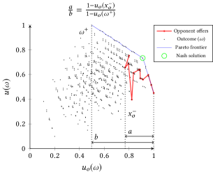
Figure 1. Visualization of Concession Rate (CR)

5.2.3. Average rate

We introduce the Average Rate (AR) that indicates the average utility an opponent has demanded as a ratio depending on the scenario. The two constants needed are the FYU ($u_{o}(\omega^{+})$) as described in the previous section and the average utility an opponent demanded ($u_{o}(\bar{x})$). The AR is a normalized ratio $AR\in[0,1]$, where $AR=0$ means that the opponent only offered his maximum outcome and $AR=1$ means that the average utility the opponent demanded is less than or equal to the FYU. We present a definition of the AR in Equation 9 and a visualization in Figure 2.

$$AR(\bar{x})=\begin{cases}1&\text{if }u_{o}(\bar{x})\leq u_{o}(\omega^{+}),\\ \frac{1-u_{o}(\bar{x})}{1-u_{o}(\omega^{+})}&\text{otherwise.}\end{cases}$$ (9)

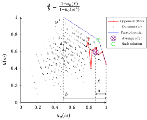
Figure 2. Visualization of Average Rate (AR)

The AR is another indication of competitiveness of the opponent based on average utility demanded instead of minimum demanded utility as the CR is.

5.2.4. Default configuration performance

According to Hutter et al. Hutter et al. (2011), the performance of any default configuration on a problem works well as a feature for that specific problem. For negotiation, this translates to the obtained utility of a hand-picked default strategy on a negotiation instance. The obtained utility is normalized and can be used as a feature for that negotiation instance.

We implement this concept as an opponent feature by selecting a default strategy and using it to obtain an agreement $\omega_{agree}$ with the opponent. We then normalize the obtained utility and use it as the Default Configuration Performance (DCP) feature. We present the formal definition of this feature in Equation 10 and a visualization in Figure 3.

$$DCP(\omega_{agree})=\begin{cases}0&\text{if }u(\omega_{agree})\leq u(\omega^{-}),\\ \frac{u(\omega_{agree})-u(\omega^{-})}{1-u(\omega^{-})}&\text{otherwise.}\end{cases}$$ (10)

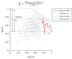
Figure 3. Visualization of Default Configuration Performance (DCP)

5.3. Opponent utility function

As can be seen in Figure 1, 2, and 3, the actual opponent utility function $u_{o}(\omega)$ is used to calculate the opponent features. SMAC is only used to configure the Dynamic Agent on the training set. As the opponent features are only used by SMAC, we can safely use the opponent’s utility function to construct those features (Equation 8, 9 and 10) without giving the Dynamic Agent an unfair advantage during testing. The Dynamic Agent always uses the predicted opponent utility $\hat{u}_{(}\omega)$ obtained through the model (Section 3.2.2), as is conventional in the ANAC.

We provide an overview of when the predicted opponent utility function and when the actual opponent utility function is used in Table 4.

	Training	Testing
$DA(\theta)$	$\hat{u}_{o}(\omega)$	$\hat{u}_{o}(\omega)$
SMAC	$u_{o}(\omega)$	N/A

Table 4. Opponent utility function usage

6. Empirical evaluation

We must set baseline configurations to compare to the result of the optimization. The basis of our Dynamic Agent is derived from a paper by Lau et al. Lau et al. (2006). Though some functionality is added, it is possible to set our agent’s strategy to resemble that of the original agent. We refer to this configuration from the literature as $\theta_{l}$, its parameters can be found in Table 5.

Another baseline strategy is added, which is configured manually, as the literature configuration is outdated. A combination of intuition, past research, and manual search, is used for this manual configuration, which we consider default method for current ANAC competitors. We present the manually configured parameters $\theta_{m}$ in Table 5 and an explanation below:

• Accepting: The acceptance condition parameters of $\theta_{l}$ set a pure $AC_{next}$ strategy with parameters $\alpha=1,\ \beta=0$. Baarslag et al. Baarslag et al. (2014) performed an empirical research on a variety of acceptance conditions and showed that there are better alternatives. We set the accepting parameters of our configuration to the best performing condition as found by Baarslag et al. Baarslag et al. (2014).

• Fitness function: Preliminary testing showed that the literature configuration concedes much faster than the average ANAC agent, resulting in a poor performing strategy. We set a more competitive parameter configuration for the fitness function by manual search, to match the competitiveness of the ANAC agents.

• Space exploration: The domain used in the paper has a relatively small set of outcomes. We increased the population size, added an extra evolution to the genetic algorithm and made some minor adjustments to cope with larger outcome spaces.

	Accepting				Fitness function			Space exploration
$\theta$	$\alpha$	$\beta$	$t_{acc}$	$\gamma$	$n$	$\delta$	$e$	$N_{p}$	$N_{t}$	$E$	$R_{c}$	$R_{m}$	$R_{e}$
$\theta_{l}$	$1$	$0$	$1$	$MAX^{W}$	$1$	$0.5$	$0.5$	$200$	$3$	$3$	$0.6$	$0.05$	$0.1$
$\theta_{m}$	$1$	$0$	$0.98$	$MAX^{W}$	$4$	$0.95$	$0.05$	$300$	$5$	$4$	$0.6$	$0.05$	$0.05$

Table 5. Baseline configurations parameters

6.1. Method

SMAC is run in embarrassingly parallel mode on a computing cluster by starting a separate SMAC process on chunks of allocated hardware. SMAC selects a negotiation instance and a configuration to evaluate on that instance and calls the negotiation environment GENIUS through a wrapper function.

Input

The training instances were created by selecting a diverse set of opponents and scenarios from the GENIUS environment. The scenarios have non-linear utility functions and vary in competitiveness and outcome space size (between 9 and 400 000). The scenario features were calculated in advance as described in Section 5.1, and the configuration space is defined in Section 3.2.

The opponent features, as defined in Section 5.2, can only be gathered by performing negotiations against the opponents. We gather these features in advance by negotiating 10 times in every instance with the manual strategy $\theta_{m}$.

Hardware & configuration budget

We perform 300 independent parallel runs of SMAC for 4 hours of wall-clock time each, on a computing cluster running Simple Linux Utility for Resource Management Yoo et al. (2003) (SLURM). To ensure consistent results, all runs were performed on Intel^® Xeon^® CPU, allocating 1 CPU core, with 2 processing threads and 12 GB RAM to each run of SMAC.

Output

Every parallel SMAC process outputs its best configuration $\theta_{inc}$ after the time budget is exhausted. As there are 300 parallel processes, a decision must be made on which of the 300 configurations to use. To do so, the SMAC random forest regression model conform Equation 6 is rebuild and used to predict the performance of every $\theta_{inc}$. The configuration with the best predicted performance is selected as best configuration $\theta_{opt}$.

6.2. Results

The configuration process as described is run three times without instance features and three times with instance features, under identical conditions. There is now a total of 8 strategies: 2 baselines $[\theta_{l},\theta_{m}]$, 3 optimized without features $[\theta_{1},\theta_{2},\theta_{3}]$, and 3 optimized with features $[\theta_{4},\theta_{5},\theta_{6}]$. An overview of the final configurations is presented in Table 6.

	Accepting				Fitness function			Space exploration
$\theta$	$\alpha$	$\beta$	$t_{acc}$	$\gamma$	$n$	$\delta$	$e$	$N_{p}$	$N_{t}$	$E$	$R_{c}$	$R_{m}$	$R_{e}$
$\theta_{l}$	$1$	$0$	$1$	$MAX^{W}$	$1$	$0.5$	$0.5$	$200$	$3$	$3$	$0.6$	$0.05$	$0.1$
$\theta_{m}$	$1$	$0$	$0.98$	$MAX^{W}$	$4$	$0.98$	$0.05$	$300$	$5$	$4$	$0.4$	$0.05$	$0.05$
$\theta_{1}$	$1.001$	$0.048$	$0.901$	$AVG^{W}$	$3$	$0.879$	$0.00183$	$345$	$10$	$4$	$0.437$	$0.003$	$0.176$
$\theta_{2}$	$1.041$	$0.001$	$0.904$	$AVG^{W}$	$4$	$0.913$	$0.00130$	$384$	$5$	$4$	$0.431$	$0.126$	$0.198$
$\theta_{3}$	$1.009$	$0.026$	$0.910$	$MAX^{W}$	$1$	$0.977$	$0.00113$	$361$	$2$	$5$	$0.279$	$0.181$	$0.072$
$\theta_{4}$	$1.032$	$0.022$	$0.931$	$AVG^{W}$	$3$	$0.914$	$0.00429$	$311$	$8$	$3$	$0.251$	$0.082$	$0.132$
$\theta_{5}$	$1.015$	$0.017$	$0.925$	$AVG^{W}$	$5$	$0.961$	$0.00105$	$337$	$5$	$3$	$0.192$	$0.090$	$0.138$
$\theta_{6}$	$1.027$	$0.022$	$0.943$	$AVG^{W}$	$3$	$0.985$	$0.00227$	$283$	$7$	$4$	$0.294$	$0.057$	$0.156$

Table 6. Configurations overview

The obtained configurations are now analyzed with an emphasis on the following three topics:

1. The influence of the instance features on the convergence of the configuration process.

2. The performance of the obtained configurations on a never before seen set of instances.

3. The performance of the best configuration in an ANAC-like bilateral tournament.

6.2.1. Influence of instance features

To study the influence of the instance features on the configuration process, we compare the strategies obtained by configuring with features and by configuring without features. Only the training set of instances is used for the performance comparison, as we are purely interested in the convergence towards a higher utility.

Every configuration is run 10 times on the set of training instances $\Pi_{train}$ and the average obtained utility is calculated by Equation 4. The results are presented in Table 7, including an improvement ratio over $\theta_{m}$.

$\theta$	$O(\theta,\Pi)$	$\frac{O(\theta,\Pi)-O(\theta_{m},\Pi)}{O(\theta_{m},\Pi)}$	Description
$\theta_{l}$	0.533	-0.307	Literature
$\theta_{m}$	0.769	0	Manually configured
$\theta_{1}$	0.785	0.020	Configured without features
$\theta_{2}$	0.770	0.000	Configured without features
$\theta_{3}$	0.792	0.029	Configured without features
$\theta_{4}$	0.800	0.040	Configured with features
$\theta_{5}$	0.816	0.060	Configured with features
$\theta_{6}$	0.803	0.044	Configured with features

Table 7. Performance of configurations on $\Pi=\Pi_{train}$

SMAC is capable of improving the performance of the Dynamic Agent above our capabilities of manual configuration. We observe that configuration without instance features potentially leads to marginal improvements on the training set. Finally, we observe that the usage of instance features leads to less variation in final configuration parameters (Table 6) and to a significant improvement of obtained utility.

6.2.2. Performance on test set

Testing the configurations on a never before seen set of opponent agents and scenarios is needed to rule out potential overfitting. We selected a diverse set of scenarios and opponents for testing, such that $|\Pi_{test}|=|A_{test}|*|S_{test}|=16*28=448$.

Every configuration is once again run 10 times on the set of training instances $\Pi_{test}$ and the average obtained utility is calculated by Equation 4. The results are presented in Table 8, including an improvement ratio over $\theta_{m}$.

$\theta$	$O(\theta,\Pi)$	$\frac{O(\theta,\Pi)-O(\theta_{m},\Pi)}{O(\theta_{m},\Pi)}$	Description
$\theta_{l}$	0.563	-0.261	Literature
$\theta_{m}$	0.763	0	Manually configured
$\theta_{1}$	0.779	0.021	Configured without features
$\theta_{2}$	0.760	-0.004	Configured without features
$\theta_{3}$	0.774	0.015	Configured without features
$\theta_{4}$	0.792	0.038	Configured with features
$\theta_{5}$	0.795	0.042	Configured with features
$\theta_{6}$	0.789	0.034	Configured with features

Table 8. Performance of configurations on $\Pi=\Pi_{test}$

It is now clear that strategy configuration without instance features is undesirable as it potentially leads to a worse performing strategy. Configuration with instance feature on the other hand, still leads to a significant performance increase on a never before seen set of negotiation instances.

6.2.3. ANAC tournament performance of best configuration

The strategy configuration method is successful in finding improved configurations, but the results are only compared against the other configurations of our Dynamic Agent. No comparison is yet made with agents build by ANAC competitors. We now compare the performance of the best configuration that we found to the ANAC agents in the test set of opponents.

We select $\theta_{5}$ as the best strategy based on performance on the training set and enter the Dynamic Agent in an ANAC-like bilateral tournament with a 60 second deadline. The Dynamic Agent is combined with the test set of opponents and scenarios. Every combination of 2 agents negotiated 10 times on every scenario, for a total amount of 38080 negotiation sessions. The averaged results are presented in Table 9. We elaborate on the performance measures found in the table:

• Utility: The utility of the agreement.

• Opp. utility: The opponent’s utility of the agreement.

• Social welfare: The sum of utilities of the agreement.

• Pareto distance: Euclidean distance of the agreement to the nearest outcome on the Pareto frontier in terms of utility.

• Nash distance: Euclidean distance of the agreement to the Nash solution in terms of utility (Equation 1).

• Agreement ratio: The ratio of negotiation sessions that result in an agreement.

Agent	Utility	Opp. utility	Social welfare	Pareto distance	Nash distance	Agreement ratio
RandomCounterOfferParty	0.440	0.957	1.398	0.045	0.415	1.000
HardlinerParty	0.496	0.240	0.735	0.507	0.754	0.496
AgentH	0.518	0.801	1.319	0.118	0.408	0.904
ConcederParty	0.577	0.848	1.425	0.047	0.358	0.964
LinearConcederParty	0.600	0.831	1.431	0.046	0.350	0.964
PhoenixParty	0.625	0.501	1.125	0.263	0.468	0.748
GeneKing	0.637	0.760	1.396	0.061	0.383	0.993
Mamenchis	0.651	0.725	1.377	0.087	0.360	0.927
BoulwareParty	0.662	0.786	1.448	0.043	0.319	0.968
Caduceus	0.677	0.486	1.163	0.241	0.453	0.784
Mosa	0.699	0.640	1.339	0.113	0.385	0.902
ParsCat2	0.716	0.671	1.386	0.108	0.286	0.904
RandomDance	0.737	0.716	1.453	0.024	0.344	0.998
ShahAgent	0.744	0.512	1.256	0.188	0.389	0.821
AgentF	0.751	0.605	1.356	0.100	0.367	0.918
SimpleAgent	0.756	0.437	1.194	0.212	0.470	0.801
$DA(\theta_{5})$	0.795	0.566	1.361	0.087	0.407	0.922

Table 9. Bilateral ANAC tournament results using $DA(\theta_{5})$ (bold = best, underline = worst)

Using the Dynamic Agent with $\theta_{5}$ results in a successful negotiation agent that is capable of winning a ANAC-like bilateral tournament by outperforming all other agents (two-tailed t-test: $p<0.001$). It managed to obtain a $\frac{0.795-0.756}{0.756}*100\%\approx 5.1\%$ higher utility than SimpleAgent, the number two in the ranking, while also outperformed it on every other performance measure.

Since the presence of our agent in the tournament also influences the performance of other agents, we also ran the full tournament without our Dynamic Agent as a sanity check. The top 5 performers of this tournament are presented in Table 10, along with their margins over the respective next lower-ranking agent in terms of utility.

Agent	Utility	Margin
Mosa	0.715	3.01%
ShahAgent	0.736	2.43%
RandomDance	0.754	0.65%
AgentF	0.759	0.01%
SimpleAgent	0.759

Table 10. Bilateral ANAC tournament without $DA(\theta_{5})$

7. Conclusion

The two main contributions of this work are (1) the success of automated configuration of negotiation strategies using a general-purpose configuration procedure (here: SMAC), and (2) an investigation of the importance of the features of negotiation settings.

7.1. Configuration

Two baseline strategies were selected for our comparison. The first configuration, $\theta_{l}$, is based on publications from which we derived the agent Lau et al. (2006); Baarslag et al. (2014). The second configuration, $\theta_{m}$, is configured based on intuition, recent literature and manual search, which we considered the default approach for current ANAC competitors. In Section 6, we automatically configured our dynamic Agent using SMAC.

The configuration based on earlier work $\theta_{l}$ Lau et al. (2006) performed poorly compared to the manually configured configuration $\theta_{m}$, and achieved 26.1% lower utility on our test set. The best automatically configured strategy $\theta_{5}$ outperformed both baseline configurations and achieved a 4.2% increase in utility compared to $\theta_{m}$. From this, we conclude that the automated configuration method is successful in outperforming manual configuration.

Our experiments show that the automated configuration method can produce a strategy that can win an ANAC-like bilateral tournament by a margin of 5.1% (Table 9). This is particularly striking when considering that without our agent, the winner of the same tournament beats the next-based agent only by a margin of 0.01%.

7.2. Features

We consider a set of features that characterizes the negotiation scenario as well as the opponent. Our empirical results indicate that when using the negotiation instance features, SMAC is able to find good configurations faster.

Overall, using SMAC in combination with instance features leads to less variation in the parameter settings between the final configurations obtained in multiple independent runs (Table 6, Table 7), as well as significant and consistent performance improvement. Furthermore, our results show that automated configuration without features does not always outperform manual configuration. Therefore, we conclude that the instance features presented in this paper are a necessary ingredient for the successful automated configuration of negotiation strategies.

7.3. Future work

For this initial step towards automated configuration of negotiation agents, the negotiation scenarios were simplified by removing the reservation utility and the discount factor. Now that we have demonstrated that our general approach can be successful, additional validation should be performed in more complex and different negotiation environments.

Over the years, it became clear that there is no single best negotiation strategy for all negotiation settings Lin et al. (2014). In this work, we have presented a method to automatically configure an effective strategy for a specific set of negotiation settings. However, if this set becomes too diverse, we inherently end up in a situation where the automatically configured best strategy may not perform too well. Future work should exploit the strategy space of the dynamic agent by extracting multiple complementary strategies for specific settings, along with an on-line selection mechanism that determines the strategy to be used in a specific instance.

References

- (1)
- Ansótegui et al. (2009) Carlos Ansótegui, Meinolf Sellmann, and Kevin Tierney. 2009. A Gender-Based Genetic Algorithm for the Automatic Configuration of Algorithms. In Principles and Practice of Constraint Programming - CP 2009, Ian P Gent (Ed.). Springer Berlin Heidelberg, Berlin, Heidelberg, 142–157.
- Aydoğan et al. (2017) Reyhan Aydoğan, David Festen, Koen V. Hindriks, and Catholijn M. Jonker. 2017. Alternating offers protocols for multilateral negotiation. In Studies in Computational Intelligence. Vol. 674. Springer, 153–167. https://doi.org/10.1007/978-3-319-51563-2_10
- Baarslag (2014) T Baarslag. 2014. What to bid and when to stop. 338 pages. https://doi.org/10.4233/uuid:3df6e234-a7c1-4dbe-9eb9-baadabc04bca
- Baarslag et al. (2015) Tim Baarslag, Reyhan Aydoğan, Koen V. Hindriks, Katsuhide Fujita, Takayuki Ito, and Catholijn M. Jonker. 2015. The Automated Negotiating Agents Competition, 2010–2015. AI Magazine 36, 4 (2015), 2010–2014. https://doi.org/10.1609/aimag.v36i4.2609
- Baarslag et al. (2013) Tim Baarslag, Mark Hendrikx, Koen Hindriks, and Catholijn Jonker. 2013. Predicting the performance of opponent models in automated negotiation. In Proceedings - 2013 IEEE/WIC/ACM International Conference on Intelligent Agent Technology, IAT 2013, Vol. 2. IEEE, 59–66. https://doi.org/10.1109/WI-IAT.2013.91
- Baarslag et al. (2011) Tim Baarslag, Koen Hindriks, and Catholijn Jonker. 2011. Towards a quantitative concession-based classification method of negotiation strategies. Lecture Notes in Computer Science (including subseries Lecture Notes in Artificial Intelligence and Lecture Notes in Bioinformatics) 7047 LNAI (2011), 143–158. https://doi.org/10.1007/978-3-642-25044-6_13
- Baarslag et al. (2014) Tim Baarslag, Koen Hindriks, and Catholijn Jonker. 2014. Effective acceptance conditions in real-time automated negotiation. Decision Support Systems 60, 1 (2014), 68–77. https://doi.org/10.1016/j.dss.2013.05.021
- Baarslag et al. (2012) Tim Baarslag, Koen Hindriks, Catholijn Jonker, Sarit Kraus, and Raz Lin. 2012. The first automated negotiating agents competition (ANAC 2010). Studies in Computational Intelligence 383, Anac (2012), 113–135. https://doi.org/10.1007/978-3-642-24696-8_7
- Balaprakash et al. (2007) Prasanna Balaprakash, Mauro Birattari, and Thomas Stützle. 2007. Improvement strategies for the F-Race algorithm: Sampling design and iterative refinement. Lecture Notes in Computer Science (including subseries Lecture Notes in Artificial Intelligence and Lecture Notes in Bioinformatics) 4771 (2007), 108–122. https://doi.org/10.1007/978-3-540-75514-2_9
- Birattari et al. (2010) Mauro Birattari, Zhi Yuan, Prasanna Balaprakash, and Thomas Stützle. 2010. F-Race and Iterated F-Race: An Overview. In Experimental Methods for the Analysis of Optimization Algorithms, Thomas Bartz-Beielstein, Marco Chiarandini, Luís Paquete, and Mike Preuss (Eds.). Springer Berlin Heidelberg, 311–336. https://doi.org/10.1007/978-3-642-02538-9_13
- Dworman et al. (1996) Garett Dworman, Steven O. Kimbrough, and James D. Laing. 1996. Bargaining by artificial agents in two coalition games: A study in genetic programming for electronic commerce. Proceedings of the First Annual Conference on Genetic Programming (1996), 54–62. http://portal.acm.org/citation.cfm?id=1595536.1595544
- Eymann (2001) T Eymann. 2001. Co-evolution of bargaining strategies in a decentralized multi-agent system. AAAI Fall 2001 Symposium on Negotiation Methods for Autonomous Cooperative Systems (2001), 126–134. http://www.aaai.org/Papers/Symposia/Fall/2001/FS-01-03/FS01-03-016.pdf
- Holland (1992) John Henry Holland. 1992. Adaptation in natural and artificial systems: an introductory analysis with applications to biology, control, and artificial intelligence. MIT press. 232 pages.
- Hutter et al. (2010) Frank Hutter, Holger H. Hoos, and Kevin Leyton-Brown. 2010. Automated configuration of mixed integer programming solvers. Lecture Notes in Computer Science (including subseries Lecture Notes in Artificial Intelligence and Lecture Notes in Bioinformatics) 6140 LNCS (2010), 186–202. https://doi.org/10.1007/978-3-642-13520-0_23
- Hutter et al. (2011) Frank Hutter, Holger H. Hoos, and Kevin Leyton-Brown. 2011. Sequential model-based optimization for general algorithm configuration. Lecture Notes in Computer Science (including subseries Lecture Notes in Artificial Intelligence and Lecture Notes in Bioinformatics) 6683 LNCS (2011), 507–523. https://doi.org/10.1007/978-3-642-25566-3_40
- Hutter et al. (2009) Frank Hutter, Holger H. Hoos, Kevin Leyton-Brown, and Thomas Stützle. 2009. ParamILS: An automatic algorithm configuration framework. Journal of Artificial Intelligence Research 36 (2009), 267–306. https://doi.org/10.1613/jair.2861
- Ilany and Gal (2016) Litan Ilany and Ya’akov Gal. 2016. Algorithm selection in bilateral negotiation. Autonomous Agents and Multi-Agent Systems 30, 4 (2016), 697–723. https://doi.org/10.1007/s10458-015-9302-8
- Klein and Lu (1989) Mark Klein and Stephen C.Y. Lu. 1989. Conflict resolution in cooperative design. Artificial Intelligence in Engineering 4, 4 (1989), 168–180. https://doi.org/10.1016/0954-1810(89)90013-7
- Lau et al. (2006) Raymond Y.K. Lau, Maolin Tang, On Wong, Stephen W. Milliner, and Yi Ping Phoebe Chen. 2006. An evolutionary learning approach for adaptive negotiation agents. International Journal of Intelligent Systems 21, 1 (2006), 41–72. https://doi.org/10.1002/int.20120
- Lin et al. (2014) Raz Lin, Sarit Kraus, Tim Baarslag, Dmytro Tykhonov, Koen Hindriks, and Catholijn M. Jonker. 2014. Genius: An integrated environment for supporting the design of generic automated negotiators. Computational Intelligence 30, 1 (2014), 48–70. https://doi.org/10.1111/j.1467-8640.2012.00463.x
- Marsa-Maestre et al. (2014) Ivan Marsa-Maestre, Mark Klein, Catholijn M. Jonker, and Reyhan Aydoǧan. 2014. From problems to protocols: Towards a negotiation handbook. Decision Support Systems 60, 1 (2014), 39–54. https://doi.org/10.1016/j.dss.2013.05.019
- Matos et al. (1998) Noyda Matos, Carles Sierra, and Nick R. Jennings. 1998. Determining successful negotiation strategies: An evolutionary approach. Proceedings - International Conference on Multi Agent Systems, ICMAS 1998 (1998), 182–189. https://doi.org/10.1109/ICMAS.1998.699048
- Nash (1950) John F. Nash. 1950. The Bargaining Problem. Econometrica 18, 2 (1950), 155. https://doi.org/10.2307/1907266
- Osborne and Rubinstein (1994) Martin J. Osborne and Ariel Rubinstein. 1994. A Course in Game Theory. (1 ed.). Vol. 1. MIT press. https://doi.org/10.2307/2554642
- Raiffa (1982) Howard Raiffa. 1982. The art and science of negotiation. Harvard University Press.
- Robinson (1990) W.N. Robinson. 1990. Negotiation behavior during requirement specification. [1990] Proceedings. 12th International Conference on Software Engineering (1990), 268–276. https://doi.org/10.1109/ICSE.1990.63633
- Rosenschein (1986) J. S. Rosenschein. 1986. Rational interaction: cooperation among intelligent agents. Ph.D. Dissertation. Stanford University, Stanford, CA, USA. http://www.osti.gov/energycitations/product.biblio.jsp?osti_id=5310977
- Rubinstein (1982) Ariel Rubinstein. 1982. Perfect Equilibrium in a Bargaining Model. Econometrica 50, 1 (1982), 97. https://doi.org/10.2307/1912531
- Smith (1980) Reid G. Smith. 1980. The Contract Net Protocol: High-Level Communication and Control in a Distributed Problem Solver. IEEE Trans. Comput. C-29, 12 (1980), 1104–1113. https://doi.org/10.1109/TC.1980.1675516
- Sycara (1988) Katia Sycara. 1988. Resolving Goal Conflicts via Negotiation. The Seventh National Conference on Artificial Intelligence (1988), 245–249. http://www.aaai.org/Papers/AAAI/1988/AAAI88-044.pdf
- Sycara-Cyranski (1985) K Sycara-Cyranski. 1985. Arguments Of Persuasion In Labour Mediation. Proceedings of the International Joint Conference on Artificial Intelligence 1 (1985), 294–296.
- Van Galen Last (2012) Niels Van Galen Last. 2012. Agent Smith: Opponent model estimation in bilateral multi-issue negotiation. Studies in Computational Intelligence 383 (2012), 167–174. https://doi.org/10.1007/978-3-642-24696-8_12
- Yoo et al. (2003) Andy B. Yoo, Morris A. Jette, and Mark Grondona. 2003. SLURM: Simple Linux Utility for Resource Management. Lecture Notes in Computer Science 2862 (2003), 44–60. https://doi.org/10.1007/10968987_3
- Zlochin et al. (2004) Mark Zlochin, Mauro Birattari, Nicolas Meuleau, and Marco Dorigo. 2004. Model-based search for combinatorial optimization: A critical survey. Annals of Operations Research 131, 1-4 (2004), 373–395. https://doi.org/10.1023/B:ANOR.0000039526.52305.af