A study on the statistical significance of mutual information between morphology of a galaxy and its large-scale environment

Abstract

A non-zero mutual information between morphology of a galaxy and its large-scale environment is known to exist in SDSS upto a few tens of Mpc. It is important to test the statistical significance of these mutual information if any. We propose three different methods to test the statistical significance of these non-zero mutual information and apply them to SDSS and Millennium Run simulation. We randomize the morphological information of SDSS galaxies without affecting their spatial distribution and compare the mutual information in the original and randomized datasets. We also divide the galaxy distribution into smaller subcubes and randomly shuffle them many times keeping the morphological information of galaxies intact. We compare the mutual information in the original SDSS data and its shuffled realizations for different shuffling lengths. Using a $t$-test, we find that a small but statistically significant (at $99.9\%$ confidence level) mutual information between morphology and environment exists upto the entire length scale probed. We also conduct another experiment using mock datasets from a semi-analytic galaxy catalogue where we assign morphology to galaxies in a controlled manner based on the density at their locations. The experiment clearly demonstrates that mutual information can effectively capture the physical correlations between morphology and environment. Our analysis suggests that physical association between morphology and environment, may extend to much larger length scales than currently believed and the information theoretic framework presented here, can serve as a sensitive and useful probe of the assembly bias and large-scale environmental dependence of galaxy properties.

1 Introduction

The role of environment on galaxy formation and evolution is one of the most complex issues in cosmology. The present day Universe is filled with billions of galaxies which are distributed across a vast network namely the ‘cosmic web’ (Bond et al., 1996) that stretches through the Universe. This spectacular network of galaxies is made up of interconnected filaments, walls and nodes which are encompassed by vast empty regions. The galaxies broadly form and evolve in these four types of environments inside the cosmic web. One can characterize the environment of a galaxy with the local density at its location. The role of local density on galaxy properties is well studied in literature (Oemler, 1974; Dressler, 1980; Goto et al., 2003; Davis & Geller, 1976; Guzzo et al., 1997; Zehavi et al., 2002; Hogg et al., 2003; Blanton et al., 2003; Park et al., 2005; Einasto, et al., 2003a; Kauffmann et al., 2004; Mouhcine et al., 2007; Koyama et al., 2013; Bamford et al., 2009). It is now well known that the galaxy properties exhibit a strong dependence on the local density of their environment. However the role of large-scale environment on the formation and evolution of galaxies still remains a debated issue.

The growth of primordial density perturbations leads to collapse of dark matter halos in a hierarchical fashion. It is now widely accepted following the seminal work by White & Rees (1978) that galaxies form at the centre of the dark matter halos by radiative cooling and condensation. One of the central postulates of the halo model (Neyman & Scott, 1952; Mo & White, 1996; Ma & Fry, 2000; Seljak, 2000; Scoccimarro & Sheth, 2001; Cooray & Sheth, 2002; Berlind & Weinberg, 2002; Yang, Mo & van den Bosch, 2003) is that the halo mass determines all the properties of a galaxy. But this need not be strictly true. The halos are assembled through accretion and merger in different parts of the cosmic web. Different accretion and merger histories of the halos across different environments leads to assembly bias (Croton, Gao & White, 2007; Gao & White, 2007; Musso, et al., 2018; Vakili & Hahn, 2019) which manifests in the clustering of these halos. The early-forming low mass halos in simulations are found to be more strongly clustered than the late-forming halos of similar mass.

The presence of beyond halo mass effect in observations, is a matter of considerable debate due to conflicting results obtained by various studies on galactic conformity and assembly bias. A study (Zehavi, et al., 2011) of the colour and luminosity dependence of galaxy clustering in SDSS find that most observed trends can be explained by halo occupation distribution (HOD) modelling within a $\Lambda$CDM cosmology. Alam, et al. (2019) study the dependence of clustering and quenching on the cosmic web using SDSS and show that the observed cosmic web dependence in the SDSS can be largely explained by HOD modelling without introducing any galaxy assembly bias. Yan, Fan & White (2013) show that the galaxy properties do not depend on the tidal environment of the cosmic web. Paranjape, Hahn & Sheth (2018) show that any observed dependence of galaxy properties on the tidal environment can be traced to those inherited from the assembly bias of their parent halos and additional effects of large-scale environment must be weak. Lin, et al. (2016) analyze the clustering of early and late forming halo samples using SDSS and find no significant evidence for assembly bias. Abbas & Sheth (2007) show that environmental effects are also present in Poisson cluster models and the halo bias in these models are surprisingly similar to the standard models of halo bias (Mo & White, 1996). A number of observations suggest that the properties of satellite galaxies are strongly correlated with the central galaxy (Weinmann et al., 2006; Kauffmann et al., 2010; Wang et al., 2010; Wang & White, 2012). Tinker, et al. (2017) study the effect of halo formation history on quenching process in central galaxies and find a statistically significant impact at high masses and no impact at low masses. Kauffmann et al. (2013) find that the star formation rates in galaxies can be correlated upto 4 Mpc. Sin, Lilly & Henriques (2017) re-examine the nature of galactic conformity presented in Kauffmann et al. (2013) and find that such effects can arise due to selection biases. Paranjape, et al. (2015) prescribed a tunable model within HOD framework to introduce varying levels of conformity in the mock galaxy catalogues and find no conclusive evidence of galaxy assembly bias on 4 Mpc. Miyatake, et al. (2016) study the halo bias of SDSS galaxy clusters using projected auto-correlation function and weak lensing and find that they differ by a factor of $1.5$, which could be a significant evidence of assembly bias. Zu, et al. (2017) study the possible origin of the discrepancy between the large scale halo bias of galaxy clusters (Miyatake, et al., 2016) and find that these differences mostly arise due to projection effects. A recent work by Kerscher (2018) reported the existence of galactic conformity out to 40 Mpc. Montero-Dorta, et al. (2017) analyze LRGs from SDSS-III BOSS survey and find a strong observational evidence of assembly bias.

Some other works (Luparello et al., 2015; Scudder et al., 2012; Pandey & Bharadwaj, 2006, 2008; Darvish et al., 2014; Filho et al., 2015) report significant dependence of the luminosity, star formation rate and metallicity of galaxies on the large-scale environment. A recent study by Lee (2018) show that both the least and most luminous elliptical galaxies in sheetlike structures inhabit the regions with highest tidal coherence. It has been shown that the large-scale environments in the cosmic web influence the mass, shape and spin of dark matter halos (Hahn et al., 2007, 2007b). A number of studies (Trujillo et al., 2006; Lee & Erdogdu, 2007; Paz et al., 2008; Jones et al., 2010; Tempel & Libeskind, 2013; Tempel et al., 2013) suggest alignment of halo shapes and spins with filaments which can extend upto $40$ Mpc (Chen, et al., 2019). In a recent study Pandey & Sarkar (2017) use information theoretic measures to show that the galaxy morphology and environment in the SDSS exhibit a synergic interaction at least upto a length scale of $\sim 30{\,h^{-1}\,{\rm Mpc}}$. A more recent study (Pandey & Sarkar, 2020) find that the fraction of red galaxies in sheets and filaments increases with the size of these large-scale structures. Any such large-scale correlations beyond the extent of the dark matter halo are unlikely to be explained by direct interactions between them. All these observations suggest that the role of environment on galaxy formation and evolution may not be limited to local density alone. The morphology and coherence of large-scale patterns in the cosmic web may play a significant role in determining the galaxy properties and their evolution.

Pandey & Sarkar (2017) use mutual information to quantify the large-scale environmental dependence of galaxy morphology. They find a non-zero mutual information between morphology of galaxies and their environment which decreases with increasing length scales but remains non-zero throughout the entire length scales probed. In the present work, we would like to test the statistical significance of mutual information between morphology and environment and study its validity and effectiveness as a measure of large-scale environmental dependence of galaxy properties for future studies.

We propose a method where we destroy the correlation between morphology and environment by randomizing the morphological classification and measure the mutual information to test its statistical significance. We also divide the data into cubes and shuffle them around many times to test how the mutual information between morphology and environment are affected by the shuffling procedure. We carry out these tests using data from the Galaxy Zoo database (Lintott, et al., 2008). Further, we carry out a controlled test using a semi-analytic galaxy catalogue (Henriques et al., 2015) based on the Millennium simulation (Springel et al., 2005). The galaxies in these mock datasets are selectively assigned morphology based on their local density. We measure the mutual information between morphology and environment in each case and try to understand the statistical significance of mutual information in the present context. The goal of the present analysis is to explore the potential of mutual information as a statistical measure to reveal the large-scale correlations between environment and morphology if any.

A $\Lambda$CDM cosmological model with $\Omega_{m0}=0.315$, $\Omega_{\Lambda 0}=0.685$ and $h=0.674$ (Planck Collaboration, et al., 2018) is used to convert redshifts to distances throughout the analysis.

2 DATA

2.1 SDSS DR16

We use data from the $16^{th}$ data release Ahumada, et al. (2019) of Sloan Digital Sky Survey (SDSS) York, et al. (2000). DR16 is the final data release of the fourth phase of SDSS which covers more than nine thousand square degrees of the sky and provides spectral information for more than two million galaxies. This includes an accumulation of data collected for new targets as well as targets from all prior data releases of SDSS. The data is downloaded through SciServer: CASjobs which is a SQL based interface for public access. We identify a contiguous region within $0^{\circ}\leq\delta\leq 60^{\circ}$ & $135^{\circ}\leq\alpha\leq 225^{\circ}$ and select all galaxies with the apparent r-band Petrosian magnitude limit $m_{r}<17.77$ within that region. Here $\alpha$ and $\delta$ are the right ascension and declination respectively. We combine the three tables SpecObjAll, Photoz and ZooSpec of SDSS database to get the required information about each of these selected galaxies. We retrieve the spectroscopic and photometric information of galaxies from the SpecObjAll and Photoz tables respectively. The ZooSpec table provides The morphological classifications for the SDSS galaxies from the Galaxy Zoo project. Galaxy zoo (Lintott, et al., 2008, 2011) is a platform where millions of registered volunteers vote for visual morphological classification of galaxies. These votes contribute in identification of galaxy morphologies through a structured algorithm. The galaxies in galaxy zoo are flagged as spiral, elliptical or uncertain depending on the vote fractions. We only consider the galaxies which are flagged as spiral or elliptical with debiased vote fraction $>0.8$ (Bamford et al., 2009). These cuts yield a total $136155$ galaxies within redshift $z<0.3$. We then construct a volume limited sample using a r-band absolute magnitude cut $M_{r}\leq-20.5$. This provides us $44049$ galaxies within $z<0.096$. The present analysis requires a cubic region. We extract a cubic region of side $145{\,h^{-1}\,{\rm Mpc}}$ from the volume limited sample which contains $14558$ galaxies. The resulting datacube consists of $11171$ spiral galaxies and $3387$ elliptical galaxies. The mean intergalactic separation of the galaxies in this sample is $\sim 6{\,h^{-1}\,{\rm Mpc}}$.

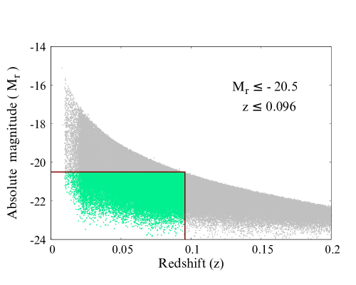
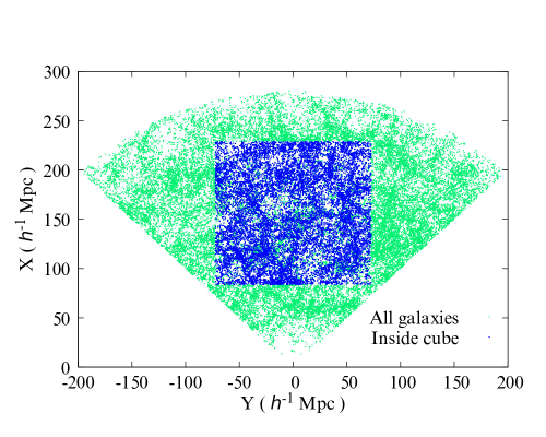
Figure 1: The top left panel shows the definition of the volume limited sample in the redshift-absolute magnitude plane. The top right panel shows the projected view of the galaxies in the entire volume limited sample (green dots) and those inside the cubic region (blue dots). The bottom left panel shows the distributions of spirals (blue dots) and ellipticals (brown dots) in the extracted datacube from the volume limited sample. The bottom right panel shows the variation in number density inside the datacube along each of the 3-axes. The number densities are computed in slices of thickness $10.36{\,h^{-1}\,{\rm Mpc}}$.

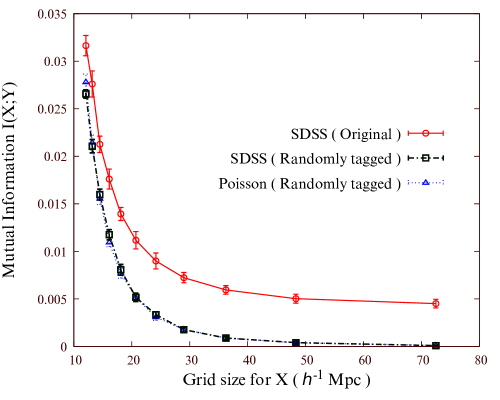
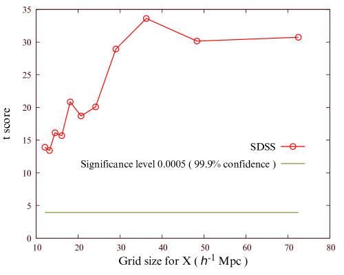
Figure 2: The left panel of this figure shows the mutual information $I(X;Y)$ as a function of length scales for the original SDSS datacube and the SDSS datacube where the morphological information of galaxies are randomized. The results for mock Poisson distribution with randomly assigned morphology are also shown together for a comparison. The $1-\sigma$ errorbars for the original SDSS data are estimated using $10$ jack-knife samples drawn from the same dataset. For the SDSS random and Poisson random datasets each, we estimate the $1-\sigma$ errobars using 10 different realizations. The right panel of this figure shows the t score as a function of length scales, obtained from a $t$-test which compares the SDSS galaxy distribution with randomized morphological classification to the SDSS galaxy distribution with actual morphological classification.

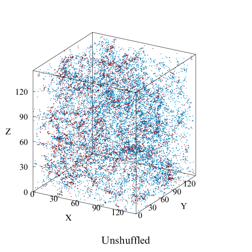
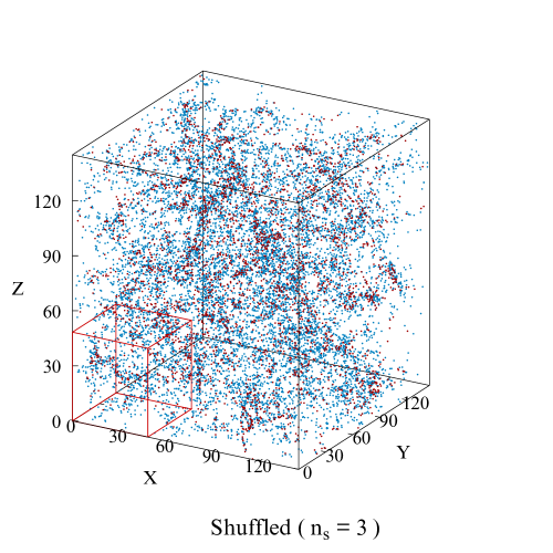
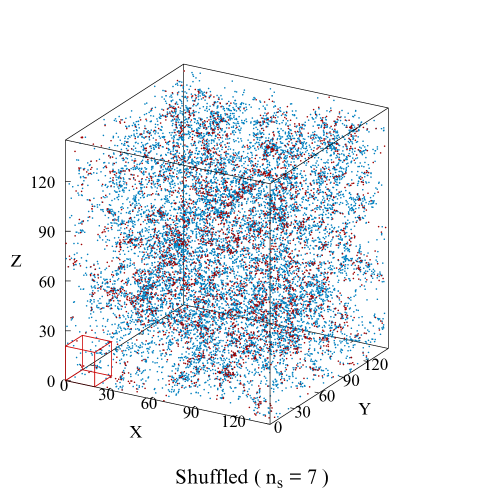
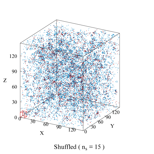
Figure 3: This figure shows the distributions of spirals (blue dots) and ellipticals (brown dots) in the original unshuffled SDSS datacube along with one realization of shuffled datacube for three different values of shuffling lengths ($l_{s}$). The value of $l_{s}$ is decided by $n_{s}$ which is the number of subcubes that would fit along each dimension. The size of shuffling units in each case is shown with a subcube (in red) at a corner of the respective shuffled realization.

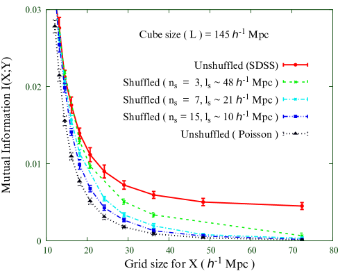
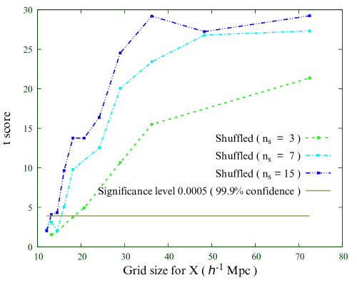
Figure 4: The left panel of this figure shows the mutual information $I(X;Y)$ as a function of length scales in the unshuffled SDSS datacube along with that from the shuffled realizations with three different shuffling length. The $1-\sigma$ errorbars shown for the unshuffled SDSS data are obtained from $10$ jack-knife samples drawn from the same dataset. For the SDSS shuffled datasets and Poisson random datasets each, the $1-\sigma$ errobars are estimated using 10 different realizations. For each shuffling length, the grid sizes are chosen so that they are not equal or integral multiples of the shuffling length and the vice versa. The right panel of this figure shows the t score at different length scales, obtained from a $t$ test comparing the shuffled distributions with the original unshuffled galaxy distribution from SDSS.

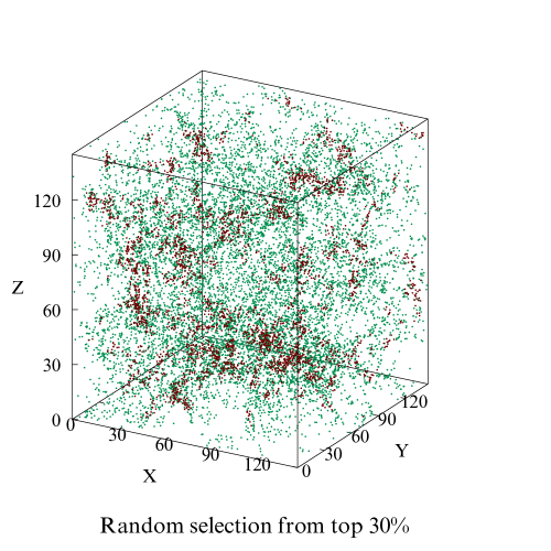
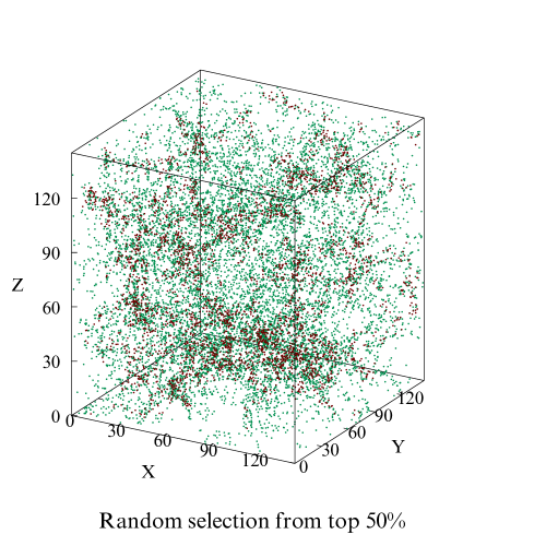
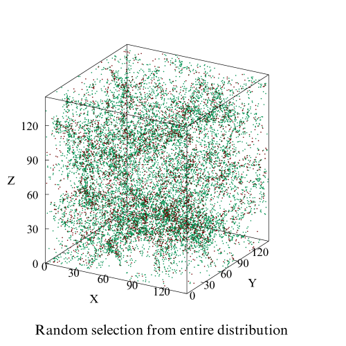
Figure 5: This figure shows the distributions of spirals (greenish dot) and ellipticals (brown dot) in a realization of the mock SDSS datacube from SAM where the galaxies are assigned morphology based on the density at their locations. The three datacubes corresponds to three different schemes for density dependent morphology assignment.

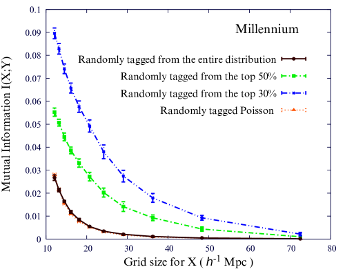
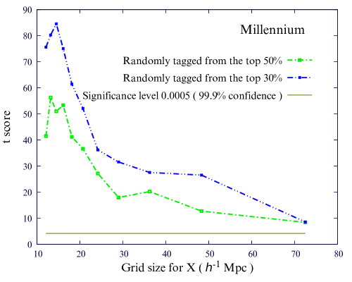
Figure 6: The left panel of this figure shows mutual information $I(X;Y)$ as a function of length scales for different morphology-density relations. $1-\sigma$ errorbars for the Millennium galaxies are estimated using data from 8 non-overlapping mock datacubes from the SAM catalogue. The $1-\sigma$ errorbars corresponding to the Poisson dataset are estimated using 8 mock datacubes containing random distributions. The right panel of this figure shows the t score at different length scales, obtained from $t$ test where we compared the distributions with density dependent morphological tagging to that without any density dependence of morphology.

2.2 Millennium Run Simulation

Galaxy formation and evolution involve many complex physical processes such as gas cooling, star formation, supernovae feedback, metal enrichment, merging and morphological evolution. The semi analytic models (SAM) of galaxy formation (White & Frenk, 1991; Kauffmann, White & Guiderdoni, 1993; Cole et al., 1994; Baugh et al., 1998; Somerville & Primack, 1999; Benson et al., 2002) is a powerful tool which parametrise these complex physical processes in terms of simple models following the dark matter merger trees over time and finally provide the statistical predictions of galaxy properties at any given epoch. In the present work, we use the data from a semi analytic galaxy catalogue (Henriques et al., 2015) derived from the Millennium run simulation (MRS) (Springel et al., 2005). Henriques et al. (2015) updated the Munich model of galaxy formation using the values of cosmological parameters from PLANCK first year data. This model provides a better fit to the observed stellar mass functions and reproduce the recent data on the abundance and passive fractions of galaxies over the redshift range $0\leq z\leq 3$ better than the other models. We use SQL to extract the required data from the Millennium database . We use the peculiar velocities of the Millennium galaxies to map them in redshift space and extract all the galaxies with $M_{r}\leq-20.5$. Finally we construct 8 mock SDSS datacubes of side $145{\,h^{-1}\,{\rm Mpc}}$ each containing a total $14558$ galaxies.

2.3 Random distributions

We simulate 10 Poisson distributions each within a cube of side $145{\,h^{-1}\,{\rm Mpc}}$. $14558$ random data points are generated within each of the 10 datacubes. For each cube, we randomly label $3387$ points as elliptical and rest of the points are labelled as spirals. The number of galaxies and the ratio of spirals to ellipticals in these random data sets are identical to that observed in the original SDSS datacube.

3 Method of analysis

3.1 Mutual information between environment and morphology

We consider a cubic region of side $L{\,h^{-1}\,{\rm Mpc}}$ extracted from the volume limited sample prepared from SDSS DR16. We subdivide the entire cube into $N_{d}$ number of $d{\,h^{-1}\,{\rm Mpc}}\times d{\,h^{-1}\,{\rm Mpc}}\times d{\,h^{-1}\,{\rm Mpc}}$ voxels. We define a discrete random variable $X$ with $N_{d}$ outcomes $\{X_{i}:i=1,...N_{d}\}$. The probability of finding a randomly selected galaxy in the $i^{th}$ voxel is $p(X_{i})=\frac{N_{i}}{N}$, where $N_{i}$ is the number of galaxies in the $i^{th}$ voxel and $N$ is the total number of galaxies in the cube. The random variable $X$ thus defines the environment of a galaxy at a specific length scale $d{\,h^{-1}\,{\rm Mpc}}$.

The information entropy (Shannon, 1948) associated with the random variable $X$ at scale $d$ is given by

$$H(X) = -\sum_{i=1}^{N_{d}}p(X_{i})\log p(X_{i})$$ (1)

$$= \log N-\frac{\sum_{i=1}^{N_{d}}N_{i}\log N_{i}}{N}$$

We use another variable $Y$ to describe the morphology of the galaxies. We have only considered the galaxies with a classified morphology and hence there are only two possible outcomes: spiral or elliptical. If the cube consists of $N_{sp}$ spiral galaxies and $N_{el}$ elliptical galaxies then the information entropy associated with $Y$ will be

$$H(Y) = -\left(\frac{N_{sp}}{N}\log\frac{N_{sp}}{N}+\frac{N_{el}}{N}\log\frac{N_{el}}{N}\right)$$ (2)

$$= \log N-\frac{N_{sp}\log N_{sp}+N_{el}\log N_{el}}{N}$$

Now having the prior information about the morphology of each of the galaxies one can determine the mutual information between morphology of the galaxies and their environment.

The mutual information $I(X;Y)$ between environment and morphology is ,

$$I(X;Y) = \sum^{N_{d}}_{i=1}\sum^{2}_{j=1}\,p(X_{i},Y_{j})\,\log\,\frac{p(X_{i},Y_{j})}{p(X_{i})p(Y_{j})}$$

$$= H(X)+H(Y)-H(X,Y)$$

$H(X)$ and $H(Y)$ are the individual entropy associated with the random variables $X$ and $Y$ respectively. The joint entropy $H(X,Y)\leq H(X)+H(Y)$ where the equality holds only when $X$ and $Y$ are independent. The joint entropy is symmetric i.e. $H(X,Y)=H(Y,X)$.

If $N_{ij}$ is the number of galaxies in the $i^{th}$ voxel that belongs to the $j^{th}$ morphological class ($j=1$ for spiral and $j=2$ for elliptical), then the joint entropy $H(X,Y)$ is given by,

$$H(X,Y) = -\sum_{i=1}^{N_{d}}\sum_{j=1}^{2}p(X_{i},Y_{j})\log p(X_{i},Y_{j})$$ (4)

$$= \log N-\frac{1}{N}\sum_{i=1}^{N_{d}}\sum_{j=1}^{2}N_{ij}\log N_{ij}$$

where

$$\sum_{i=1}^{N_{d}}\sum_{j=1}^{2}N_{ij}=N$$ (5)

Here $p(X_{i},Y_{j})=p(X_{i}|Y_{j})p(Y_{j})=\frac{N_{ij}}{N}$ is the joint probability derived from the conditional probability using Bayes’ theorem.

The mutual information between two random variables measures the reduction in uncertainty in the knowledge of one random variable given the knowledge of other. A higher value of mutual information between two random variables convey a greater degree of association between the two random variables. One specific advantage of mutual information over the traditional tools like covariance analysis is that it does not require any assumptions regarding the nature of the random variables and their relationship.

3.2 Randomizing the morphological classification of galaxies

We consider each of the SDSS galaxies in the datacube and randomly identify them as spirals and ellipticals leaving aside their actual morphology. We randomly pick $3387$ SDSS galaxies and tag them as ellipticals. Rest of the galaxies in the SDSS datacube are labelled as spirals. The number of spirals and ellipticals in the resulting distribution thus remains same as the original distribution.

We generate 10 such datacubes with randomly assigned galaxy morphology from the original SDSS datacube and measure the mutual information between environment and morphology in each of them. We would like to compare the mutual information $I(X;Y)$ measured in the original SDSS data with that from the SDSS dataset with randomly assigned morphology to study the statistical significance of $I(X;Y)$ and its scale dependence.

3.3 Shuffling the spatial distribution of galaxies

We divide the SDSS datacube of side $L{\,h^{-1}\,{\rm Mpc}}$ into $N_{c}=n_{s}^{3}$ smaller subcubes of size $l_{s}=\frac{L}{n_{s}}{\,h^{-1}\,{\rm Mpc}}$. Each of these smaller subcubes along with all the galaxies within them are rotated around three different axes by different angles which are random multiples of $90^{\circ}$. The rotated subcubes are then randomly interchanged with any other subcubes inside the datacube. This process of arbitrary rotation followed by random swapping is repeated for $100\times N_{c}$ times to generate a Shuffled realization (Bhavsar & Ling, 1988) from the original SDSS datacube. We carry out the shuffling procedure for three different choices $n_{s}=3$, $n_{s}=7$ and $n_{s}=15$ which corresponds to shuffling length $l_{s}=48.33{\,h^{-1}\,{\rm Mpc}}$, $l_{s}=20.71{\,h^{-1}\,{\rm Mpc}}$ and $l_{s}=9.67{\,h^{-1}\,{\rm Mpc}}$ respectively. We generate 10 shuffled realizations for each values of the shuffling length ($l_{s}$). Our goal is to compare the mutual information $I(X;Y)$ measured in the original SDSS data with that from the shuffled datasets to test the statistical significance of $I(X;Y)$ on different length scales.

3.4 Simulating different morphology-density correlations

The morphology-density relation is a well known phenomenon which indicates that environment play a crucial role in deciding galaxy morphology. We would like to test whether mutual information $I(X;Y)$ can capture the strength of morphology-density relation in the galaxy distribution. We construct a set of SDSS mock datacubes from a semi analytic galaxy catalogues as discussed in Section 2.2.

We compute the local number density at the location of each galaxies using $k^{th}$ nearest neighbour method (Casertano & Hut, 1985). We find the distance to the the $k^{th}$ nearest neighbour to each galaxy. The local number density around a galaxy is estimated as,

$$n_{k}=\frac{k-1}{V(r_{k})}$$ (6)

Here $r_{k}$ is the distance to the $k^{th}$ nearest neighbour and $V(r_{k})=\frac{4}{3}\pi r_{k}^{3}$. We have used $k=10$ in this analysis.

Our goal is to test if $I(X;Y)$ can capture the degree and nature of correlation between environment (X) and morphology (Y). The elliptical galaxies are known to reside preferentially in denser environments. Each mock SDSS datacubes from the SAM contains a total $14558$ galaxies. We would like to assign a morphology to each of these galaxies. To do so, we first sort the number density at the locations of galaxies in a descending order. We consider three different schemes which are as follows,

(i) We randomly label $3387$ galaxies as ellipticals from the top 30% high density locations and consider the rest of the $11171$ galaxies as spirals.

(ii) We randomly label $3387$ galaxies as ellipticals from top 50% high density locations and consider the rest of the $11171$ galaxies as spirals.

(iii) We randomly label $3387$ galaxies as ellipticals irrespective of their local density and consider the rest of the $11171$ galaxies as spirals.

The morphology-density relation in case (i) is stronger than case (ii) and there is no morphology-density relation in case (iii). We would like to test if mutual information $I(X;Y)$ can correctly capture the degree of association between environment and morphology in these distributions.

3.5 Testing statistical significance of the difference in mutual information with $t$ test

We use an equal variance $t$-test which can be used when both the datasets consists of same number of samples or have a similar variance. We calculate the $t$ score at each length scale using the following formula,

$$t=\frac{|\bar{X_{1}}-\bar{X_{2}}|}{\sigma_{s}\sqrt{\frac{1}{n_{1}}+\frac{1}{n_{2}}}}$$ (7)

where $\sigma_{s}=\sqrt{\frac{(n_{1}-1)\sigma_{1}^{2}+(n_{2}-1)\sigma_{2}^{2}}{n_{1}+n_{2}-2}}$, $\bar{X_{1}}$ and $\bar{X_{1}}$ are the average values, $\sigma_{1}$ and $\sigma_{2}$ are the standard deviations, $n_{1}$ and $n_{2}$ are the number of datapoints associated with the two datasets at any given lengthscale.

We would like to test the null hypothesis that the average value of mutual information in the original and randomized or shuffled distribution at a given lengthscale are not significantly different. We find that randomizing or shuffling the data always leads to a reduction in the mutual information between morphology and environment. We use a one-tailed test with significance level $\alpha=0.0005$ which corresponds to a confidence level of $99.9\%$. The degrees of freedom in this test is $(n_{1}+n_{2}-2)$. The same test is also applied to asses the statistical significance of $I(X;Y)$ in mock datasets where a morphology-density relation is introduced in a controlled manner. We compute the $t$ score at each length scale using Equation 7 and determine the associated $p$ value to test the statistical significance.

Table 1: This table shows the $t$ score and the associated $p$ value at each length scale when we compare the mutual information between actual SDSS data and SDSS data with randomized morphological information.

Grid size ( ${\,h^{-1}\,{\rm Mpc}}$ )	$t$ score	$p$ value
$12.08$	$13.911$	$2.26\times 10^{-11}$
$13.18$	$13.417$	$4.10\times 10^{-11}$
$14.50$	$16.125$	$1.90\times 10^{-12}$
$16.11$	$15.692$	$3.02\times 10^{-12}$
$18.12$	$20.853$	$2.34\times 10^{-14}$
$20.71$	$18.698$	$1.53\times 10^{-13}$
$24.17$	$20.088$	$4.46\times 10^{-14}$
$29.00$	$28.934$	$7.59\times 10^{-17}$
$36.25$	$33.613$	$5.36\times 10^{-18}$
$48.33$	$30.151$	$3.67\times 10^{-17}$
$72.50$	$30.736$	$2.61\times 10^{-17}$

Table 2: This table shows the $t$ score and the associated $p$ value at each length scale when we compare the mutual information between actual SDSS data and its shuffled realizations for different shuffling lengths. The grid size for each $n_{s}$ is chosen in a such a way so that the shuffling length is not equal or an integral multiple of the grid size.

Grid size	$n_{s}=3$		$n_{s}=7$		$n_{s}=15$
( ${\,h^{-1}\,{\rm Mpc}}$ )	$t$ score	$p$ value	$t$ score	$p$ value	$t$ score	$p$ value
$12.08$	-	-	$2.196$	$2.07\times 10^{-2}$	$2.029$	$2.88\times 10^{-2}$
$13.18$	$1.559$	$6.82\times 10^{-2}$	$3.148$	$2.78\times 10^{-3}$	$4.097$	$3.38\times 10^{-4}$
$14.50$	$1.967$	$3.24\times 10^{-2}$	$2.037$	$2.83\times 10^{-2}$	$4.324$	$2.04\times 10^{-4}$
$16.11$	-	-	$5.064$	$4.04\times 10^{-5}$	$9.656$	$7.63\times 10^{-9}$
$18.12$	$3.794$	$6.64\times 10^{-4}$	$9.806$	$6.03\times 10^{-9}$	$13.765$	$2.69\times 10^{-11}$
$20.71$	$4.928$	$5.43\times 10^{-5}$	-	-	$13.762$	$2.70\times 10^{-11}$
$24.17$	-	-	$12.536$	$1.24\times 10^{-10}$	$16.367$	$1.48\times 10^{-12}$
$29.00$	$10.667$	$1.64\times 10^{-9}$	$20.061$	$4.57\times 10^{-14}$	$24.534$	$1.38\times 10^{-15}$
$36.25$	$15.510$	$3.68\times 10^{-12}$	$23.429$	$3.09\times 10^{-15}$	$29.184$	$6.52\times 10^{-17}$
$48.33$	-	-	$26.795$	$2.94\times 10^{-16}$	$27.235$	$2.20\times 10^{-16}$
$72.50$	$21.376$	$1.52\times 10^{-14}$	$27.325$	$2.08\times 10^{-16}$	$29.234$	$6.33\times 10^{-17}$

Table 3: This table shows the $t$ score and the associated $p$ value at each length scale when we compare the mutual information between mock datasets with and without a morphology-density relation.

Grid size	Random selection from top 30%		Random selection from top 50%
( ${\,h^{-1}\,{\rm Mpc}}$ )	$t$ score	$p$ value	$t$ score	$p$ value
$12.08$	$75.590$	$5.46\times 10^{-20}$	$41.511$	$2.32\times 10^{-16}$
$13.18$	$80.264$	$2.36\times 10^{-20}$	$56.285$	$3.35\times 10^{-18}$
$14.50$	$84.539$	$1.14\times 10^{-20}$	$50.987$	$1.33\times 10^{-17}$
$16.11$	$75.073$	$6.01\times 10^{-20}$	$53.361$	$7.04\times 10^{-18}$
$18.12$	$61.435$	$9.88\times 10^{-19}$	$41.186$	$2.59\times 10^{-16}$
$20.71$	$52.083$	$9.87\times 10^{-18}$	$36.618$	$1.32\times 10^{-15}$
$24.17$	$36.197$	$1.55\times 10^{-15}$	$27.185$	$8.10\times 10^{-14}$
$29.00$	$31.549$	$1.04\times 10^{-14}$	$17.937$	$2.34\times 10^{-11}$
$36.25$	$27.540$	$6.77\times 10^{-14}$	$20.213$	$4.65\times 10^{-12}$
$48.33$	$26.512$	$1.14\times 10^{-13}$	$12.707$	$2.23\times 10^{-9}$
$72.50$	$8.541$	$3.17\times 10^{-7}$	$8.379$	$3.98\times 10^{-7}$

4 Results

4.1 Effects of randomizing the morphological classification

We show the mutual information $I(X;Y)$ between environment and morphology as a function of length scale in the SDSS datacube in left panel of Figure 2 which shows that the morphology of the SDSS galaxies and their large-scale environment share a small non-zero mutual information throughout the entire length scale. The result for the SDSS datasets with randomly assigned morphology is also shown in the same panel for a comparison. This shows that there is a significant reduction in $I(X;Y)$ at each length scale due to the randomization of morphological information of the SDSS galaxies. We find that a finite non-zero mutual information still persists at each length scale even after the randomization of morphology. To understand its origin, we also measure the mutual information measured in the Poisson datacubes with randomly assigned morphology and show them together in the left panel of Figure 2. Interestingly, we find that the non-zero mutual information between $X$ and $Y$ in the Poisson distributions are nearly same as the SDSS datacube with randomly assigned morphology.

The information entropy $H(X)$ associated with environment at each length scale $d$ remains unchanged, as the position of each galaxies in the resulting distribution remains same as the original SDSS distribution. There would be also no change in the information entropy $H(Y)$ associated with morphology of the galaxies as the number of spirals and ellipticals remains the same after the randomization. However this procedure would change the joint entropy $H(X,Y)$. The randomization of morphological classification would turn the joint probability distribution to a product of the two individual probability distribution i.e. $p(X_{i},Y_{j})=p(X_{i})p(Y_{j})$. The adopted procedure is thus expected to destroy any existing correlations between environment and morphology and consequently any non-zero mutual information between environment and morphology should ideally disappear after the randomization.

However in left panel of Figure 2, we find that $I(X;Y)$ does not reduce to zero after the randomization of morphology of the SDSS galaxies. This residual nonzero mutual information can be explained by the results obtained from the Poisson datacubes with randomly assigned morphology. The results show that $I(X;Y)$ in the Poisson datacubes with randomly assigned morphology and SDSS datacube with randomly assigned morphology are nearly the same. This suggests that a part of the measured mutual information arises due to the finite and discrete nature of the galaxy sample. The origin of this residual information is thus non-physical in nature and should be properly taken into account during such analysis.

The reduction in $I(X;Y)$ due to the randomization of morphology suggests that a part of the measured mutual information $I(X;Y)$ must have some physical origin. Interestingly, left panel of Figure 2 shows that randomization leads to a reduction in the mutual information at each length scale. We test the statistical significance of these differences at each length scale using a $t$ test. We show the $t$ score at each length scale in the right panel of Figure 2. The critical $t$ score at $99.9\%$ confidence level for $18$ degrees of freedom are also shown in the same panel. The $t$ score and the associated $p$ value at each length scale are tabulated in Table 1. We find a strong evidence against the null hypothesis which suggests that the differences in the mutual information $I(X;Y)$ in the two distributions are statistically significant at $99.9\%$ confidence level for the entire length scales probed. This clearly indicates that the association between environment and morphology is not limited to only the local environment but extends to environments on larger length-scales.

4.2 Effects of shuffling the spatial distribution of galaxies

We divide the SDSS datacube into a number of regular subcubes using different values of $l_{s}$ as discussed in Section 3.3 and shuffle them many times to generate a set of shuffled realizations for each shuffling length. The Figure 3 shows the distributions of ellipticals (brown dots) and spirals (blue dots) in the original unshuffled SDSS datacube along with one realization of the shuffled datacubes for each shuffling length. The size of the shuffling units used to shuffle the data in each case are shown with a red subcube at the corner of the respective shuffled datacubes. A comparison of the shuffled datacubes with the original SDSS datacube clearly shows that the coherent features visible in the actual data on larger length scales progressively disappears with the increasing shuffling length. It may be noted that both the measurement of $I(X;Y)$ and shuffling requires us to divide the datacube into a number of subcubes. In each case, we choose the shuffling lengths and the grid sizes so that the shuffling length is not equal or integral multiple of grid size or vice versa. This must be ensured to avoid any spurious correlations in $I(X;Y)$.

We compare the mutual information $I(X;Y)$ in the original and shuffled datasets in the left panel of Figure 4. For each shuffled datasets we observe a reduction in $I(X;Y)$ at different length scales. A smaller reduction in $I(X;Y)$ is observed at smaller length scales whereas a relatively larger reduction in $I(X;Y)$ is seen on larger length scales.

It may be noted that the morphological information of galaxies remain intact after shuffling the data. The shuffling procedure keeps the clustering at scales below $l_{s}$ nearly identical to the original data but eliminates all the coherent spatial features in the galaxy distribution on scales larger than $l_{s}$. Shuffling is thus expected to diminish any existing correlations between environment and morphology. Measuring the mutual information between environment and morphology in the original SDSS data and its shuffled versions allows us to address the statistical significance of $I(X;Y)$. The mutual information is expected to reduce by a greater amount on scales above the shuffling length $l_{s}$ because shuffling destroys nearly all the coherent patterns beyond this length scale. On the other hand, we expect a relatively smaller reduction in $I(X;Y)$ below the shuffling length $l_{s}$. This can be explained by the fact that most of the coherent features in the galaxy distribution below length scale $l_{s}$ survive the shuffling procedure. However some of the coherent features which extend upto $l_{s}$ but lie across the subcubes would be destroyed by shuffling. Shuffling may also produce a small number of spatial features which are the product of pure chance alignments. These random features are unlikely to introduce any physical correlations between environment and morphology. A comparison of $I(X;Y)$ between the original and shuffled data at different length scales for different shuffling length thus reveal the statistical significance of the degree of association between environment and morphology on different length scales.

We find that $I(X;Y)$ decreases monotonically at all length scales with decreasing shuffling lengths. Figure 4 shows that $I(X;Y)$ for $n_{s}=15$ or $l_{s}\sim 10{\,h^{-1}\,{\rm Mpc}}$ still lies above the values that are expected for an identical Poisson random distributions. A greater reduction in $I(X;Y)$ on larger length scales for each shuffling length considered suggests that the mutual information between environment and morphology is statistically significant on these length scales. $I(X;Y)$ in actual data and shuffled data for different shuffling lengths do not differ much on smallest length scale as the coherent structures on these length scales are nearly intact in all the shuffled datasets. However when shuffled with smaller values of $l_{s}$, greater number of coherent structures on larger length scales are lost. This explain why reduction in $I(X;Y)$ increases with decreasing shuffling length.

We employ a $t$ test to test the statistical significance of the observed differences in $I(X;Y)$ in original and all shuffled datasets at different length scales. The $t$ score and the corresponding $p$ value at each length scale are tabulated in Table 2. The $t$ score for the shuffled datasets for three different shuffling length are shown as a function of length scale in the right panel of Figure 4. We find that the differences in $I(X;Y)$ in the shuffled and unshuffled SDSS data are statistically significant at $99.9\%$ confidence level at nearly the entire length scale probed.

We find a weak evidence against the null hypothesis for all the shuffling lengths at smaller length scales. This arises due to the fact that the coherence between environment and morphology are retained on smaller scales when the data is shuffled with a comparable or larger shuffling lengths. However we note that a considerable reduction in $I(X;Y)$ can occur even below the shuffling length for $n_{s}=7$ and $n_{s}=3$. A subset of the coherent features extending below the shuffling length may lie across the subcubes used to shuffle the data. These coherent structures will be destroyed by the shuffling procedure even when they are smaller than the shuffling length. The number of such coherent structures which belongs to this particular group is expected to increase with the size of the subcubes due to their larger boundary.

The results shown in Figure 4 thus indicates that the association between environment and morphology is certainly not limited to their local environment but extends throughout the length scales probed in this analysis.

4.3 Effects of different morphology-density correlations

In Figure 5, we show the distributions of spirals and ellipticals in mock SDSS datacubes from SAM. We show one distribution for each of the simulated morphology-density relations.

We show the mutual information $I(X;Y)$ as a function of length scales for the three different density-morphology relation in the left panel of Figure 6. When the elliptical are randomly selected from the entire distribution irrespective of their density then we do not expect any mutual information between morphology and environment. The non-zero mutual information in this case is just an outcome of the finite and discrete nature of the distributions. We find that the results for this case is identical to that expected for a Poisson distribution with same ratio of spirals to ellipticals.

However when ellipticals are preferentially selected from denser regions, the mutual information between morphology and environment rises above the values that are expected for a Poisson random distribution. The figure Figure 6 shows that mutual information $I(X;Y)$ is significantly higher than Poisson distribution when galaxies are randomly tagged as elliptical from the top $50\%$ high density positions. We find that the mutual information between morphology and environment increase further to much higher values when galaxies are randomly identified as ellipticals from the top $30\%$ high density regions. We note a change in $I(X;Y)$ at all lengthscales upto $50{\,h^{-1}\,{\rm Mpc}}$. A larger change in $I(X;Y)$ is observed on smaller length scales whereas the change in $I(X;Y)$ becomes gradually smaller on larger length scales. This indicates that the morphology-density relations simulated here, become weaker on larger length scales.

We use a $t$ test to asses the statistical significance of the differences in $I(X;Y)$ in the mock datasets with and without a morphology-density relation. We tabulate the $t$ score and the corresponding $p$ value at each length scale for the two mock datasets in Table 3. In the right panel of Figure 6, we show the $t$ score as a function of length scales in two mock datasets with different morphology-density relation. The results suggest that a statistically significant difference ($99.9\%$ confidence level) exists between the datasets with and without a morphology-density relation. Interestingly, these differences persist throughout the entire length scale probed in the analysis. This indicates that the correlation between environment and morphology is not limited to the local environment but extends to larger length scales.

The morphology-density relations considered here are too simple in nature. In this experiment, we find that the mutual information between morphology and environment decreases monotonically with increasing length scales. Contrary to this, the SDSS observations show that mutual information initially decreases with increasing length scales and nearly plateaus out at larger length scales. The schemes used for the morphology-density relation in this experiment are not realistic in nature. But they clearly shows that mutual information can effectively capture the degree of association between morphology and environment and such a relation may extend upto larger length scales.

5 Conclusions

In the present work, we aim to test the statistical significance of mutual information between morphology of a galaxy and its environment. The morphology-density relation is a well known phenomenon which has been observed in the galaxy distribution. The relation suggests that the ellipticals are preferentially found in denser regions of galaxy distribution whereas spirals are sporadically distributed across the fields. It is important to understand the role of environment in galaxy formation and evolution. The local density at the location of a galaxy is very often used to characterize its environment. It is believed that the environmental dependence of galaxy properties can be mostly explained by the local density alone. The mutual information between environment and morphology for SDSS galaxies has been studied by Pandey & Sarkar (2017) where they find that a non-zero mutual information between morphology and environment persists throughout the entire length scale probed. They show that the mutual information between environments on different length scales may introduce such correlations between environment and morphology observed on larger length scales. We would like to critically examine the statistical significance of the observed non-zero mutual information between morphology and environment on different length scales. We propose three different methods to asses the statistical significance of mutual information. These methods also help us to understand the relative importance of environment on different length scales in deciding the morphology of galaxies.

Three different tests are carried out in the present analysis. In the first case, we randomize the morphological information about the SDSS galaxies without affecting their spatial distribution. In the second case, we shuffle the spatial distribution of the SDSS galaxies without affecting their morphological classification. Both these tests show that the mutual information between morphology and environment are statistically significant at $99.9\%$ confidence level throughout the entire length scales probed in this analysis. We find that a small non-zero mutual information can be observed even in a random distribution without any existing physical correlations between environment and morphology. This non-zero value originates from the finite and discrete nature of the distribution. Interestingly, the mutual information between environment and morphology in the SDSS datacube is significantly larger than the randomized datasets throughout the entire length scales probed. Shuffling the SDSS datacube also affect the mutual information between environment and morphology in a statistically significant way at nearly the entire length scales considered. This suggests that the association between morphology and environment continues upto a larger length scales and these correlations must have a physical origin. In a third test, we construct a set of mock SDSS datacubes from the semi analytic galaxy catalogue where we assign morphology to the simulated galaxies based on the density at their locations. We vary the strength of the simulated morphology-density relation and measure mutual information between environment and morphology in each case. Our results suggest that mutual information effectively capture the degree of association between environment and morphology in these mock datasets.

We extend our analysis to dark matter halo sample from Millennium simulation (see Appendix A) where we investigate if the angular momentum of dark matter halos display any large-scale correlations at fixed halo mass. The analysis shows that statistically significant correlations are observed only for the halos in the mass range $\sim 10^{11}-10^{12}M_{\odot}$. The assembly bias is known to be more pronounced at low masses ($\sim 10^{12}M_{\odot}$) and the observed correlations could be a signature of assembly bias. But we could not confirm this due to a wider variation of halo mass in this mass range. Choosing a narrower range around this halo mass does not provide us sufficient number of dark matter halos within the specific volume required for the present analysis. The present analysis also suggests that the observed large-scale correlations between morphology and environment is small but statistically more significant than that observed between the angular momentum of dark matter halos and their environment.

Besides the halo assembly bias, the rich baryonic physics may also play an important role, which allow much more complicated interactions between galaxies and their environment. The effects of local density on morphology of galaxies is understood in terms of various types of galaxy interactions, ram pressure stripping and quenching of star formation. These processes may play a dominant role in shaping the morphology of a galaxy. However they may not be the only factors which decides the morphology of a galaxy. The presence of large-scale coherent features like filaments, sheets and voids may induce large-scale correlations between the observed galaxy properties and their environment. Further studies may reveal if any new physical processes are required to explain such large-scale correlations. In any case, we need to understand the physical origin of such correlations and if required, incorporate them in the models of galaxy formation. Most studies employ correlation functions to study the assembly bias. Here, we speculate that the information theoretic framework presented in this paper, might serve as a more sensitive probe of galaxy assembly bias than traditional correlation functions.

Every statistical measure have their pros and cons. One particular drawback of mutual information is that it does not tell us the direction of the relation between two random variables i.e. the measured mutual information does not provide us the simple information that the ellipticals and spirals are preferentially distributed in high density and low density regions respectively. But the mutual information reliably captures the degree of association between any two random variables irrespective of the nature of their relationship. So in the present context, mutual information can be an effective and powerful tool to quantify the degree of influence that environment imparts on morphology across different length scales. The amplitude of mutual information quantify the strength of correlation between morphology and environment on different length scales. It also helps us to probe the length scales upto which the morphology of a galaxy is sensitive to its environment.

One can also study the mutual information between environment and any other galaxy property to understand the influence of environment on that property at various length scales. The relative influence of environment on different galaxy properties on any given length scale may provide useful inputs for the galaxy formation models. Finally we note that mutual information between environment and a galaxy property is a powerful and effective tool which can be used successfully for the future studies of large-scale environmental dependence of galaxy properties.

6 Data availability

The data underlying this article are available in https://skyserver.sdss.org/casjobs/ and https://www.mpa.mpa-garching.mpg.de/millennium/. The datasets were derived from sources in the public domain: https://www.sdss.org/, http://zoo1.galaxyzoo.org and https://www.mpa.mpa-garching.mpg.de/millennium/.

7 ACKNOWLEDGEMENT

The authors thank an anonymous reviewer for useful comments and suggestions which helped us to improve the draft. SS would like to thank UGC, Government of India for providing financial support through a Rajiv Gandhi National Fellowship. BP would like to acknowledge financial support from the SERB, DST, Government of India through the project CRG/2019/001110. BP would also like to acknowledge IUCAA, Pune for providing support through associateship programme.

The authors would like to thank the SDSS team and Galaxy Zoo team for making the data public. Funding for the Sloan Digital Sky Survey IV has been provided by the Alfred P. Sloan Foundation, the U.S. Department of Energy Office of Science, and the Participating Institutions. SDSS-IV acknowledges support and resources from the Center for High-Performance Computing at the University of Utah. The SDSS web site is www.sdss.org.

SDSS-IV is managed by the Astrophysical Research Consortium for the Participating Institutions of the SDSS Collaboration including the Brazilian Participation Group, the Carnegie Institution for Science, Carnegie Mellon University, the Chilean Participation Group, the French Participation Group, Harvard-Smithsonian Center for Astrophysics, Instituto de Astrofísica de Canarias, The Johns Hopkins University, Kavli Institute for the Physics and Mathematics of the Universe (IPMU) / University of Tokyo, the Korean Participation Group, Lawrence Berkeley National Laboratory, Leibniz Institut für Astrophysik Potsdam (AIP), Max-Planck-Institut für Astronomie (MPIA Heidelberg), Max-Planck-Institut für Astrophysik (MPA Garching), Max-Planck-Institut für Extraterrestrische Physik (MPE), National Astronomical Observatories of China, New Mexico State University, New York University, University of Notre Dame, Observatário Nacional / MCTI, The Ohio State University, Pennsylvania State University, Shanghai Astronomical Observatory, United Kingdom Participation Group, Universidad Nacional Autónoma de México, University of Arizona, University of Colorado Boulder, University of Oxford, University of Portsmouth, University of Utah, University of Virginia, University of Washington, University of Wisconsin, Vanderbilt University, and Yale University.

The Millennium Simulation data bases (Lemson & Virgo Consortium, 2006) used in this paper and the web application providing online access to them were constructed as part of the activities of the German Astrophysical Virtual Observatory.

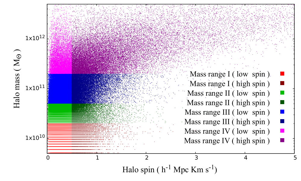
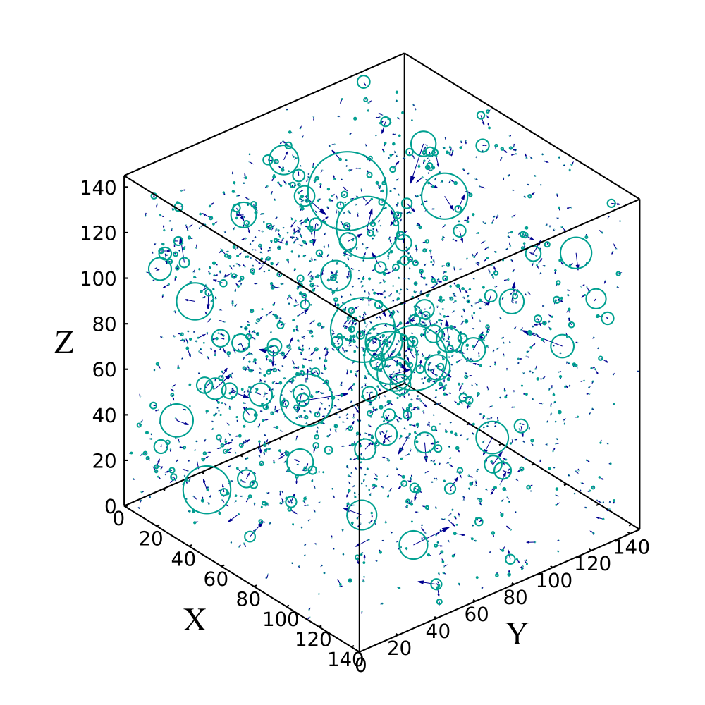
Figure 7: The left panel of the figure shows the distribution of halo spin in the four mass bins. The right panel of the figure shows the spatial distribution of 2000 dark matter halos randomly selected from the entire population. In this panel, each green circle represents a dark matter halo and the blue arrows attached to each circle represent the angular momentum vector associated with the halo. The radii of the circles are proportional to the masses and the lengths of the arrows are proportional to the magnitudes of the angular momentum of the dark matter halos. This is shown as a visual representation of the distribution of dark matter halos and their angular momentum. We have used only the spatial distribution of the halo centers in our analysis.

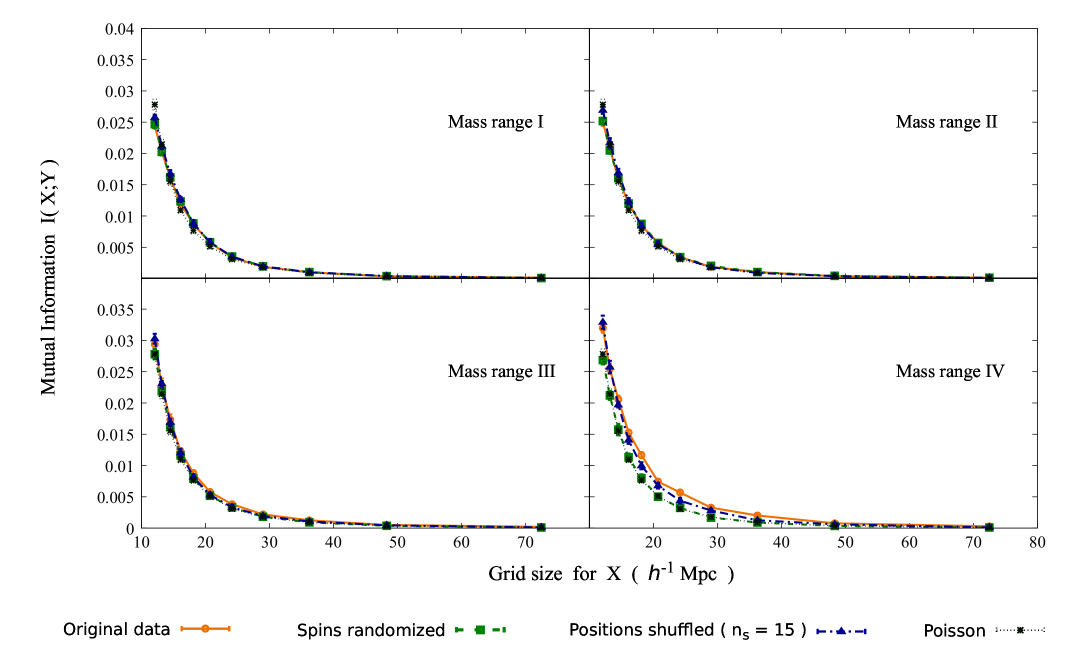
Figure 8: The different panels of this figure show the mutual information between the environment of a dark matter halo and its spin angular momentum for $4$ different mass bins. The results after randomization of the halo spins and shuffling of the spatial distributions ($n_{s}=15$) are also shown together in each panel. We also show the results for mock Poisson samples with randomly assigned spin angular momentum in each case. The $1-\sigma$ errorbars are obtained from 10 subsamples analyzed in each mass bin.

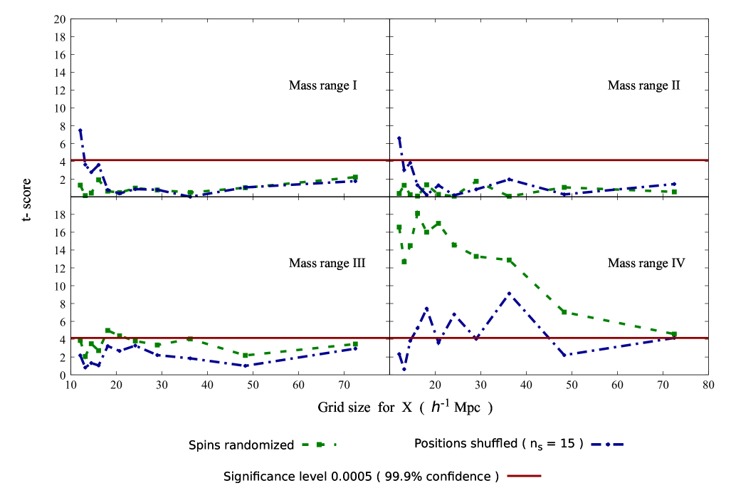
Figure 9: The different panels of this figure show the t score at different length scales, for the randomized and shuffled distributions in four different halo mass ranges.

Table 4: This table shows the four bins which is used to classify the dark matter halos.

Mass range I ( in $M_{\odot}$ unit )	:   $5\times 10^{9}\leq M\leq 2\times 10^{10}$
Mass range II ( in $M_{\odot}$ unit )	:   $2\times 10^{10}\leq M\leq 5\times 10^{10}$
Mass range III ( in $M_{\odot}$ unit )	:   $5\times 10^{10}\leq M\leq 2\times 10^{11}$
Mass range IV ( in $M_{\odot}$ unit )	:   $2\times 10^{11}\leq M\leq 5\times 10^{12}$

Appendix A Mutual information between the environment and angular momentum of dark matter halos

In this section, we would like to extend our analysis to dark matter halos using the Millennium halo catalogue. We download the data from MPAHaloTrees table of Millennium database using a SQL query. We retrieve the virial mass, angular momentum (in $h^{-1}$Mpc Km s^-1 units ) and 3 dimensional position and velocities of all the dark matter halos. We map the spatial distribution of the halos from real space to redshift space and extract a cubic region of size $145{\,h^{-1}\,{\rm Mpc}}$. These halos are then divided into four different bins depending on their masses, which are defined in Table 4. We construct $10$ mock samples corresponding to each mass bin. $14558$ halos are randomly selected for $10$ times for each mass bin. Each mock sample thus contains $14558$ dark matter halos distributed within a cubic region of size $145{\,h^{-1}\,{\rm Mpc}}$.

Our goal is to perform an analysis with the dark matter halos to test the large-scale environmental dependence of halo spins. The analysis is analogous to the study we carried out for the SDSS galaxies. We use the magnitude of angular momentum of the dark matter halos to classify them into two different groups. The distribution of the angular momentum ($\omega$) of the dark matter halos in different mass bins are shown in the left panel of Figure 7. Only the dark matter halos with $0<\omega\leq 5$ are considered in this analysis. We use a critical value $\omega_{c}=0.5$ to divide the halos in two different classes. The choice of $\omega_{c}$ is somewhat arbitrary. We choose this value to have significant number of halos in both the high and low angular momentum states. Halos with $\omega\leq\omega_{c}$ are termed as low spin halos whereas the ones with $\omega_{c}<\omega\leq 5$ are labelled as high spin halos.

In order to randomize the angular momentum of the halos, we randomly select pairs of halos and swap their spin tags without altering their positions. The number of low and high spin halos remains unchanged after such randomization. For each mock sample, we randomly identify $100\times 14558$ pairs and interchange their spin states. Any correlation between the environment of a halo and its spin is expected to be destroyed by this operation.

We then shuffle the spatial distribution of the dark matter halos keeping their angular momentum unchanged. We consider the smallest shuffling length ($n_{s}=15$) used for the analysis with SDSS galaxies. Higher values of shuffling lengths would be necessary only if there is a significant change in the mutual information introduced by this shuffling length.

We calculate the mutual information for the randomized and shuffled distributions of dark matter halos in each mass range.

In Figure 8, we show the mutual information between the environment of a halo and its angular momentum as a function of length scale for four different mass bins. We find a small nonzero mutual information between environment and angular momentum which respectively extend upto $30{\,h^{-1}\,{\rm Mpc}}$ and $50{\,h^{-1}\,{\rm Mpc}}$ in the first two and last two mass bins. We compare these mutual information with those obtained for the randomized and shuffled distributions in each mass bin. We find that randomizing the spins and shuffling the data do not introduce any noticeable change in the measured mutual information between angular momentum and environment in the first two halo mass bins. The fact that the actual mutual information coincides with that from randomized, shuffled and Poisson data at all scales suggests that these non-zero mutual information do not have any physical origin. They purely arise due to finite and discrete nature of the distributions. However, we observe that randomization and shuffling change the mutual information in the mass bins III and IV. We asses the statistical significance of the differences in each mass bin using $t$- test. The results are shown in different panels of Figure 9. Clearly the low mass bins (bin I and II) do not show a statistically significant change in the mutual information over nearly the entire length scale. The statistical significance of the differences gradually increases with halo mass (bin III and IV) as can be seen in the two bottom panels of Figure 9. A statistically significant difference ($99.9\%$ confidence) is observed over most of the length scales for the halos in mass range IV.

This analysis shows that for smaller mass halos, there are no clear association between the angular momentum of dark matter halos and their large-scale environment. A statistically significant correlation between these variables are observed only for the relatively more massive dark matter halos in mass bin IV. The assembly bias is expected to be more significant for halo mass $\sim 10^{12}M_{\odot}$ which are included in bin IV. So these correlations, may in principle originate from assembly bias. Alternatively, they may be a manifestation of a wider variation of halo mass in bin IV. Unfortunately, we could not verify this due to lack of sufficient number of halos within the chosen volume when a narrow mass range is opted for bin IV. We also repeat our analysis with different values of $\omega_{c}$ and recover the same trend. Finally, we note that the correlations between morphology of SDSS galaxies and their large-scale environment are more pronounced than the associations detected between angular momentum of dark matter halos and their environment.

References

- Abbas & Sheth (2007) Abbas U., Sheth R. K., 2007, MNRAS, 378, 641
- Ahumada, et al. (2019) Ahumada R., et al., 2019, arXiv, arXiv:1912.02905
- Alam, et al. (2019) Alam S., Zu Y., Peacock J. A., Mandelbaum R., 2019, MNRAS, 483, 4501
- Bamford et al. (2009) Bamford, S. P., Nichol, R. C., Baldry, I. K., et al. 2009, MNRAS, 393, 1324
- Baugh et al. (1998) Baugh, C.M., Cole, S., Frenk, C.S. & Lacey, C.G. 1998, ApJ, 498, 504
- Benson et al. (2002) Benson, A.J., Lacey, C.G., Baugh, C.M., Cole, S. & Frenk, C.S. 2002, MNRAS, 333, 156
- Berlind & Weinberg (2002) Berlind, A., Weinberg, D.H. 2002, ApJ, 575, 587
- Bhavsar & Ling (1988) Bhavsar, S. P. & Ling, E. N. 1988, ApJ Letters, 331, L63
- Blanton et al. (2003) Blanton, M. R., et al. 2003, ApJ, 594, 186
- Bond et al. (1996) Bond J. R., Kofman L., Pogosyan D. 1996, Nature, 380, 603
- Casertano & Hut (1985) Casertano S., Hut P., 1985, ApJ, 298, 80
- Chen, et al. (2019) Chen Y.-C., Ho S., Blazek J., He S., Mandelbaum R., Melchior P., Singh S., 2019, MNRAS, 485, 2492
- Cole et al. (1994) Cole, S., Aragon-Salamanaca, A., Frenk, C.S., Navarro, J.F., Zepf, S.E. 1994, MNRAS, 271, 781
- Cooray & Sheth (2002) Corray, A., Sheth, R.K., 2002, Phys. Rep., 371, 1
- Croton, Gao & White (2007) Croton D. J., Gao L., White S. D. M., 2007, MNRAS, 374, 1303
- Dressler (1980) Dressler, A., 1980, ApJ, 236, 351
- Davis & Geller (1976) Davis, M., & Geller, M.J., 1976, ApJ, 208, 13
- Darvish et al. (2014) Darvish, B., Sobral, D., Mobasher, B., et al. 2014, ApJ, 796, 51
- Einasto, et al. (2003a) Einasto, J., Hütsi, G., Einasto, M., Saar, E., Tucker, D. L., Müller, V., Heinämäki, P., & Allam, S. S. 2003, A&A, 405, 425
- Lee & Erdogdu (2007) Lee, J., & Erdogdu, P. 2007, ApJ, 671, 1248
- Filho et al. (2015) Filho, M. E., Sánchez Almeida, J., Muñoz-Tuñón, C., et al. 2015, ApJ, 802, 82
- Gao, Springel & White (2005) Gao L., Springel V., White S. D. M., 2005, MNRAS, 363, L66
- Gao & White (2007) Gao L., White S. D. M., 2007, MNRAS, 377, L5
- Goto et al. (2003) Goto, T., Yamauchi, C., Fujita, Y., Okamura, S., Seikiguchi, M., Smail, I. Bernardi, M., & Gomez, P.L., 2003, MNRAS, 346, 601
- Guzzo et al. (1997) Guzzo, L., Strauss, M.A., Fisher, K.B., Giovanelli, R., & Haynes, M.P., 1997, ApJ, 489, 37
- Hahn et al. (2007) Hahn, O., Porciani, C., Carollo, C. M., & Dekel, A. 2007, MNRAS, 375, 489
- Hahn et al. (2007b) Hahn, O., Carollo, C. M., Porciani, C., & Dekel, A. 2007, MNRAS, 381, 41
- Henriques et al. (2015) Henriques, B. M. B., White, S. D. M., Thomas, P. A., et al. 2015, MNRAS, 451, 2663
- Hogg et al. (2003) Hogg, D. W., et al. 2003, ApJ Letters, 585, L5
- Hoyle et al. (2002) Hoyle, F., et al. 2002, ApJ, 580, 663
- Jones et al. (2010) Jones, B. J. T., van de Weygaert, R., & Aragón-Calvo, M. A. 2010, MNRAS, 408, 897
- Kauffmann, White & Guiderdoni (1993) Kauffmann, G., White, S.D.M. & Guiderdoni, B. 1993, MNRAS, 264, 201
- Kauffmann et al. (2004) Kauffmann, G., White, S. D. M., Heckman, T. M., et al. 2004, MNRAS, 353, 713
- Kauffmann et al. (2010) Kauffmann, G., Li, C., & Heckman, T. M. 2010, MNRAS, 409, 491
- Kauffmann et al. (2013) Kauffmann, G., Li, C., Zhang, W., & Weinmann, S. 2013, MNRAS, 430, 1447
- Kerscher (2018) Kerscher M., 2018, A&A, 615, A109
- Koyama et al. (2013) Koyama, Y., Smail, I., Kurk, J., et al. 2013, MNRAS, 434, 423
- Lemson & Virgo Consortium (2006) Lemson G., Virgo Consortium . the ., 2006, arXiv, astro-ph/0608019
- Lee (2018) Lee J., 2018, ApJ, 867, 36
- Lintott, et al. (2008) Lintott, C. J., Schawinski, K., Slosar, A., et al. 2008, MNRAS, 389, 1179
- Lintott, et al. (2011) Lintott, C., Schawinski, K., Bamford, S., et al. 2011, MNRAS, 410, 166
- Lin, et al. (2016) Lin Y.-T., et al., 2016, ApJ, 819, 119
- Luparello et al. (2015) Luparello, H. E., Lares, M., Paz, D., et al. 2015, MNRAS, 448, 1483
- Ma & Fry (2000) Ma, C.P., Fry, J.N. 2000, ApJ, 543, 503
- Miyatake, et al. (2016) Miyatake H., More S., Takada M., Spergel D. N., Mandelbaum R., Rykoff E. S., Rozo E., 2016, PhRvL, 116, 041301
- Mo & White (1996) Mo, H. J., & White, S. D. M. 1996, MNRAS, 282, 347
- Mouhcine et al. (2007) Mouhcine, M., Baldry, I. K., & Bamford, S. P. 2007, MNRAS, 382, 801
- Montero-Dorta, et al. (2017) Montero-Dorta A. D., et al., 2017, ApJL, 848, L2
- Musso, et al. (2018) Musso M., Cadiou C., Pichon C., Codis S., Kraljic K., Dubois Y., 2018, MNRAS, 476, 4877
- Neyman & Scott (1952) Neyman, J., & Scott, E. L. 1952, ApJ, 116, 144
- Oemler (1974) Oemler A., 1974, ApJ, 194, 1
- Pandey & Bharadwaj (2006) Pandey, B., & Bharadwaj, S. 2006, MNRAS, 372, 827
- Pandey & Bharadwaj (2008) Pandey, B., & Bharadwaj, S. 2008, MNRAS, 387, 767
- Pandey & Sarkar (2017) Pandey, B., & Sarkar, S. 2017, MNRAS, 467, L6
- Pandey & Sarkar (2020) Pandey, B., & Sarkar, S. 2020, Submitted to MNRAS, arxiv:2002.08400
- Paranjape, et al. (2015) Paranjape A., Kovač K., Hartley W. G., Pahwa I., 2015, MNRAS, 454, 3030
- Paranjape, Hahn & Sheth (2018) Paranjape A., Hahn O., Sheth R. K., 2018, MNRAS, 476, 5442
- Park et al. (2005) Park, C., et al. 2005, ApJ, 633, 11
- Paz et al. (2008) Paz, D. J., Stasyszyn, F., & Padilla, N. D. 2008, MNRAS, 389, 1127
- Planck Collaboration, et al. (2018) Planck Collaboration, et al., 2018, arXiv, arXiv:1807.06209
- Scoccimarro & Sheth (2001) Scoccimarro, R., Sheth, R. 2001, ApJ, 329, 629
- Scudder et al. (2012) Scudder, J. M., Ellison, S. L., & Mendel, J. T. 2012, MNRAS, 423, 2690
- Seljak (2000) Seljak, U. 2000, MNRAS, 318, 203
- Shannon (1948) Shannon, C. E. 1948, Bell System Technical Journal, 27, 379-423, 623-656
- Sin, Lilly & Henriques (2017) Sin L. P. T., Lilly S. J., Henriques B. M. B., 2017, MNRAS, 471, 1192
- Springel et al. (2005) Springel et al. 2006, Nature, 435, 629
- Somerville & Primack (1999) Somerville, R.S. & Primack, J.R. 1999, MNRAS, 310, 1087
- Tempel & Libeskind (2013) Tempel, E., & Libeskind, N. I. 2013, ApJ Letters, 775, L42
- Tempel et al. (2013) Tempel, E., Stoica, R. S., & Saar, E. 2013, MNRAS, 428, 1827
- Tinker, et al. (2017) Tinker J. L., Wetzel A. R., Conroy C., Mao Y.-Y., 2017, MNRAS, 472, 2504
- Trujillo et al. (2006) Trujillo, I., Carretero, C., & Patiri, S. G. 2006, ApJ Letters, 640, L111
- Vakili & Hahn (2019) Vakili M., Hahn C., 2019, ApJ, 872, 115
- Wang et al. (2010) Wang, Y., Park, C., Hwang, H. S., & Chen, X. 2010, ApJ, 718, 762
- Wang & White (2012) Wang, W., & White, S. D. M. 2012, MNRAS, 424, 2574
- Weinmann et al. (2006) Weinmann, S. M., van den Bosch, F. C., Yang, X., & Mo, H. J. 2006, MNRAS, 366, 2
- White & Rees (1978) White, S. D. M., & Rees, M. J. 1978, MNRAS, 183, 341
- White & Frenk (1991) White, S. D. M. & Frenk, C. S. 1991, ApJ, 379, 52
- Yan, Fan & White (2013) Yan H., Fan Z., White S. D. M., 2013, MNRAS, 430, 3432
- Yang, Mo & van den Bosch (2003) Yang, X., Mo, H.J., van den Bosch, F.C. 2003, MNRAS, 339, 1057
- York, et al. (2000) York D. G., et al., 2000, AJ, 120, 1579
- Zehavi et al. (2002) Zehavi, I., et al. 2002, ApJ,571,172
- Zehavi, et al. (2011) Zehavi I., et al., 2011, ApJ, 736, 59
- Zu, et al. (2017) Zu Y., Mandelbaum R., Simet M., Rozo E., Rykoff E. S., 2017, MNRAS, 470, 551