Flat phase of polymerized membranes at two-loop order

Abstract

We investigate two complementary field-theoretical models describing the flat phase of polymerized – phantom – membranes by means of a two-loop, weak-coupling, perturbative approach performed near the upper critical dimension $D_{uc}=4$, extending the one-loop computation of Aronovitz and Lubensky [Phys. Rev. Lett. 60, 2634 (1988)]. We derive the renormalization group equations within the modified minimal substraction scheme, then analyze the corrections coming from two-loop with a particular attention paid to the anomalous dimension and the asymptotic infrared properties of the renormalization group flow. We finally compare our results to those provided by nonperturbative techniques used to investigate these two models.

I Introduction

Fluctuating surfaces are ubiquitous in physics (see, e.g., Refs.Nelson et al. (2004); Bowick and Travesset (2001)). One meets them within the context of high-energy physics Polyakov (1987); David (1989); Wheater (1994); See the contribution of F. David in [1] , initially through high-temperature expansions of lattice gauge theories, then in the large-$N$ limit of gauge theories, in two-dimensional quantum gravity, in string theory as world-sheet of string and, finally, in brane theory. They also occur as a fundamental object of biophysics where surfaces – called in this context membranes – constitute the building blocks of living cells such as erythrocyte Schmidt et al. (1993); Bowick and Travesset (2001). Last but not least, fluctuating surfaces – or membranes – have provided, in condensed matter physics, an extremely suitable model to describe both qualitatively and quantitatively sheets of graphene Novoselov et al. (2004, 2005) or graphenelike materials (see, e.g., Katsnelson (2012) and references therein).

Two types of membranes should be distinguished regarding their critical or, more generally, long-distance properties: fluid membranes and polymerized membranes See the contribution of D. R. Nelson in Ref.[1] ; D. R. Nelson (2002). The specificity of fluid membranes is that the molecules are essentially free to diffuse inside the structure. The consequence of this lack of fixed connectivity is the absence of elastic properties. As a result, the free energy of the membrane depends only on its shape – its curvature – and not on a specific coordinate system. Early studies de Gennes and Taupin (1982); Peliti and Leibler (1985); Helfrich (1985) have shown that strong height – out-of-plane – fluctuations occur in such systems in such a way that the normal-normal correlation functions exponentially decay with the distance over a typical persistence length $\xi\sim e^{4\pi\kappa/T}$ in a way similar to what happens in the two-dimensional $O(N)$ model. As a consequence, there is no long-range orientational order in fluid membranes – that are always crumpled – in agreement with the Mermin-Wagner theorem Mermin and Wagner (1966).

Polymerized – or tethered – membranes are more remarkable. Indeed due to the fact that molecules are tied together through a potential, they display a fixed internal connectivity giving rise to elastic – shearing and stretching – contributions to the free energy. It has been substantiated that, in these conditions, the coupling between the out-of-plane and in-plane fluctuations leads to a drastic reduction of the former Nelson and Peliti (1987). This makes possible the existence of a phase transition between a disordered crumpled phase at high temperatures and an ordered flat phase with long-range order between the normals at low-temperatures Aronovitz and Lubensky (1988); David and Guitter (1988); Guitter et al. (1989); M. Paczuski and M. Kardar and D. R. Nelson (1988); Aronovitz et al. (1989); Nelson et al. (2004), analogous to that occurring in ferro/antiferro magnets – see, however, below. Although the nature – first or second order – of this crumpled-to-flat transition is still under debate J.-P. Kownacki and Diep (2002); H. Koibuchi and N. Kusano and A. Nidaira and K. Suzuki and M. Yamada (2004); H. Koibuchi and T. Kuwahata (2005); J.-P. Kownacki and Mouhanna (2009); H. Koibuchi and A. Shobukhov (2014); Essafi et al. (2014); U. Satoshi and H. Koibuchi (2016); R. Cuerno, R. Gallardo Caballero, A. Gordillo-Guerrero, P. Monroy and J. J. Ruiz-Lorenzo (2016) and the mere existence of a crumpled phase for realistic, i.e., self-avoiding Bowick et al. (2001), membranes seems to be compromised, there is no doubt about the existence of a stable flat phase.

Let us consider a $D$-dimensional membrane embedded in the $d$-dimensional Euclidean space. The location of a point on the membrane is realized by means of a $D$-dimensional vector ${\bf x}$ whereas a configuration of the membrane in the Euclidean space is described through the embedding ${\bf x}\to{\bf R}({\bf x})$ with ${\bf R}\in\mathbb{R}^{d}$. One assumes the existence of a low temperature, flat phase, defined by ${\bf R}^{0}({\bf x)}=({\bf x},{\bf 0}_{d_{c}})$ where ${\bf 0}_{d_{c}}$ is the null vector of co-dimension $d_{c}=d-D$ and one decomposes the field $\bf{R}$ into $\bf{R}(\bm{x)}=[{\bf x}+{\bf u}({\bf x}),{\bf h}({\bf x})]$ where ${\bf u}$ and ${\bf h}$ represent $D$ longitudinal – phonon – and $d-D$ transverse – flexural – modes, respectively. The action of a flat phase configuration ${\bf R}$ is given by Nelson and Peliti (1987); Aronovitz and Lubensky (1988); David and Guitter (1988); Aronovitz et al. (1989); Guitter et al. (1988, 1989)

$$\begin{array}[]{ll}S[{\bf R}]=\displaystyle\int\text{d}^{D}x&\displaystyle\left\{{\kappa\over 2}\big{(}\Delta{\bf R}\big{)}^{2}+{\lambda\over 2}\,u_{ii}^{2}+{\mu}\,u_{ij}^{2}\right\}\end{array}$$ (1)

where $u_{ij}$ is the strain tensor that parametrizes the fluctuations around the flat phase configuration ${\bf R}^{0}({\bf x)}$: $u_{ij}={1\over 2}(\partial_{i}{\bf R}.\partial_{j}{\bf R}-\partial_{i}{\bf R}^{0}.\partial_{j}{\bf R}^{0})={1\over 2}(\partial_{i}{\bf R}.\partial_{j}{\bf R}-\delta_{ij})$. In Eq. (1), $\kappa$ is the bending rigidity constant whereas $\lambda$ and $\mu$ are the Lamé coefficients; stability considerations require that $\kappa$, $\mu$, and the bulk modulus $B=\lambda+2\mu/D$ be all positive.

The most remarkable fact arising from the analysis of (1) is that, in the flat phase, the normal-normal correlation functions display long-range order from the upper critical ($uc$) dimension $D_{uc}=4$ down to the lower critical ($lc$) dimension $D_{lc}<2\$Aronovitz and Lubensky (1988); Aronovitz et al. (1989). While in apparent contradiction with the Mermin-Wagner theorem Mermin and Wagner (1966), this result can be explained in the following way. At long distances, or low momenta, typically given by $\displaystyle q\ll\sqrt{\mu/\kappa},\sqrt{\lambda/\kappa}$, the term $\big{(}\Delta{\bf u}\big{)}^{2}$ in (1) can be neglected with respect to the terms of the type $(\partial_{i}u_{j})^{2}$ entering in the strain tensor $u_{ij}$, which are, thus, promoted to the rank of kinetic terms of the field $u$ I. V. Gornyi, V. Yu. Kachorovskii and A. D. Mirlin (2015). It follows immediately from power counting considerations that the nonlinear term in the phonon field ${\bf u}$ appearing in $u_{ij}$, i.e. $\partial_{i}u_{k}\partial_{j}u_{k}$, is irrelevant; it can thus also be discarded. Under these assumptions the stain tensor $u_{ij}$ is given by:

$$u_{ij}\simeq{1\over 2}\left[\partial_{i}u_{j}+\partial_{j}u_{i}+\partial_{i}{\bf h}.\partial_{j}{\bf h}\right]\ .$$ (2)

It follows that action (1) is now quadratic in the phonon field ${\bf u}$ and one can integrate over it exactly. This leads to an effective action depending only on the flexural field ${\bf h}$. In Fourier space, this effective action reads Le Doussal and Radzihovsky (1992); P. Le Doussal and L. Radzihovsky (2018)

$$S_{\text{eff}}[{\bf h}\,]=\frac{\kappa}{2}\,\int_{\bf k}\,k^{4}\,|{\bf h}(\bf k)|^{2}+$$

$$+\frac{1}{4}\,\int_{{\bf k}_{1},{\bf k}_{2},{\bf k}_{3},{\bf k}_{4}}{\bf h}({\bf k}_{1})\cdot{\bf h}({\bf k}_{2})\,R_{ab,cd}({\bf q})\,k_{1}^{a}\,k_{2}^{b}\,k_{3}^{c}\,k_{4}^{d}\,\,{\bf h}({\bf k}_{3})\cdot{\bf h}({\bf k}_{4})\,,$$ (3)

where $\int_{\bf k}=\int d^{D}{k}/(2\pi)^{D}$ and ${\bf q}={\bf k}_{1}+{\bf k}_{2}=-{\bf k}_{3}-{\bf k}_{4}$. The fourth order, ${\bf q}$-transverse tensor, $R_{ab,cd}({\bf q})$ is given by Le Doussal and Radzihovsky (1992); P. Le Doussal and L. Radzihovsky (2018)

$$R_{ab,cd}({\bf q})={\mu\,(D\lambda+2\mu)\over\lambda+2\mu}N_{ab,cd}({\bf q})+\mu\,M_{ab,cd}({\bf q})$$ (4)

where one has defined the two mutually orthogonal tensors:

$$\begin{array}[]{ll}&N_{ab,cd}({\bf q})=\displaystyle{1\over D-1}\,P_{ab}^{T}({\bf q})\,P_{cd}^{T}({\bf q})\\ \\ &M_{ab,cd}({\bf q})=\displaystyle{1\over 2}\,\big{[}P_{ac}^{T}({\bf q})\,P_{bd}^{T}({\bf q})+P_{ad}^{T}({\bf q})\,P_{bc}^{T}({\bf q})\big{]}-N_{ab,cd}({\bf q})\end{array}$$

where $P_{ab}^{T}({\bf q})=\delta_{ab}-q_{a}q_{b}/{\bf q}^{2}$ is the transverse projector. Note that, in $D=2$, the tensor $M_{ab,cd}$ vanishes identically and the effective action (3) is parametrized by only one coupling constant which turns out to be proportional to Young’s modulus Nelson and Peliti (1987); Le Doussal and Radzihovsky (1992); P. Le Doussal and L. Radzihovsky (2018): $K_{0}=4\mu(\lambda+\mu)/(\lambda+2\mu)$. The key point is that the momentum-dependent interaction (4) is nonlocal and gives rise to a phonon-mediated interaction between flexural modes which is of the long-range kind. More precisely, this interaction contains terms such that the product $R(|{\bf x}-{\bf y}|)|{\bf x}-{\bf y}|^{2}$ is not an integrable function in $D=2$ as required by the Mermin-Wagner theorem Mermin and Wagner (1966) (see Coquand (2019) for a detailed discussion). This flat phase is characterized by power-law behaviour for the phonon-phonon and flexural-flexural modes correlation functions Aronovitz and Lubensky (1988); Guitter et al. (1988); Aronovitz et al. (1989); Guitter et al. (1989):

$$G_{uu}(q)\sim q^{-(2+\eta_{u})}\hskip 8.5359pt{\hbox{and}}\hskip 8.5359ptG_{hh}(q)\sim{q^{-(4-\eta)}}$$ (5)

where $\eta$ and $\eta_{u}$ are nontrivial anomalous dimensions. In fact, it follows from Ward identities associated with the remaining partial rotation invariance of (1) – see below – that $\eta$ and $\eta_{u}$ are not independent quantities and one has $\eta_{u}=4-D-2\eta$ Aronovitz and Lubensky (1988); Guitter et al. (1988); Aronovitz et al. (1989); Guitter et al. (1989). Interestingly, Eq. (5) provide also an implicit equation for the lower critical dimension $D_{lc}$ defined as the dimension below which there is no more distinction between phonon and flexural modes. One gets from Eq. (5): $D_{lc}-2+\eta(D_{lc})=0$ Peliti and Leibler (1985); Aronovitz and Lubensky (1988); Aronovitz et al. (1989). It results from this expression that the lower critical dimension $D_{lc}$, as well as the associated anomalous dimension $\eta(D_{lc})$, are no longer given by a power-counting analysis around a Gaussian fixed point, as it occurs for the $O(N)$ model, but by a nontrivial computation of fluctuations. This implies, in particular, that there is no well-defined perturbative expansion of the flat phase theory near the lower critical dimension $D_{lc}$ based on the study of a nonlinear $\sigma$ – hard-constraints – model David and Guitter (1988).

On the other hand, the soft-mode, Landau-Ginzburg-Wilson, model (1) does not suffer from the same kind of pathology; a standard, $\epsilon$-expansion about the upper critical dimension $D_{uc}$ is feasible and has been performed at leading order, a long-time ago, in the seminal works of Aronovitz et al. Aronovitz and Lubensky (1988); Aronovitz et al. (1989) and Guitter et al. Guitter et al. (1988, 1989) who have determined the renormalization group (RG) equations and the properties of the flat phase near $D=4$. This perturbative approach faces, however, several drawbacks that explain why it has not been pushed forward until now: (i) It involves an intricate momentum and tensorial structure of the propagators and vertices that render the diagrammatic extremely rapidly growing in complexity with the order of perturbation Coquand et al. (2020a). (ii) The dimension of physical membranes, $D=2$, is “far away” from $D_{uc}$. Clearly, high orders of the perturbative series, followed by suitable resummation techniques, are needed to get quantitatively trustable results. The difficulty of carrying such a task is, however, increased by the first drawback. (iii) The massless theory is manageable with current modern techniques whereas, with the $1/q^{4}$–form of the flexural mode propagator $G_{hh}$ in (5), one apparently faces the problem of dealing with infrared divergences. (iv) The use of the dimensional regularization and, more precisely, the modified minimal substraction ($\overline{\rm MS}$) scheme, which is by far the most convenient one, can enter in conflict with the $D$-dependence of physical quantities or properties – see below.

In this context, several nonperturbative methods – with respect to the parameter $\epsilon=4-D$ – have been employed in order to tackle the physics directly in $D=2$. Among them, the $1/d_{c}$ expansion have been early performed at leading order David and Guitter (1988); Guitter et al. (1988); Aronovitz et al. (1989); Guitter et al. (1989); I. V. Gornyi, V. Yu. Kachorovskii and A. D. Mirlin (2015) and, very recently, at next-to-leading order D. R. Saykin, I. V. Gornyi, V. Yu. Kachorovskii and I. S. Burmistrov (2020). An improvement of the $1/d_{c}$ approximation that consists in replacing, within this last approach, the bare propagator and vertices by their dressed and screened counterparts leads to the so-called self-consistent screening approximation (SCSA) that has also been used at leading Le Doussal and Radzihovsky (1992); K. V. Zakharchenko, R. Roldán, A. Fasolino and M. I. Katsnelson (2010); R. Roldán, A. Fasolino, K. V. Zakharchenko, and M. I. Katsnelson (2011); P. Le Doussal and L. Radzihovsky (2018) and next-to-leading order Gazit (2009). Finally, a technique working in all dimensions $D$ and $d$, called nonperturbative renormalization group (NPRG) – see below – has been employed to investigate various kinds of membranes at leading order of the so-called derivative expansion J.-P. Kownacki and Mouhanna (2009); Essafi et al. (2011, 2014); Coquand and Mouhanna (2016); Coquand et al. (2018); Coquand et al. (2020b) and within an approach taking into account the full derivative dependence of the action F. L. Braghin and N. Hasselmann (2010); N. Hasselmann and F. L. Braghin (2011). Therefore, within the whole spectrum of approaches used to investigate the properties of the flat phase of membranes, it is only for the weak-coupling perturbative approach that the next-to-leading order is still missing (see however A. Mauri and M.I. Katsnelson (2020)). This is clearly a flaw as the subleading corrections of any approach generally provide valuable insights on the structure of the whole theory. They also convey useful information about the accuracy of complementary approaches.

We propose here to fill this gap and to investigate the properties of the flat phase of polymerized membranes at two-loop order in the coupling constants, near $D_{uc}=4$, considering successively the flexural-phonon, two-field, model (1) and then the flexural-flexural, effective model (3). We compute the RG functions of these two models, analyze their fixed points and compute the corresponding anomalous dimensions. Finally, we compare these results together and, then, with those obtained from nonperturbative methods. Note that, due to the length of the computations and expressions involved, we restrict here ourselves to the main results; details will be given in a forthcoming publication Coquand et al. (2020a).

II The two-field model

II.1 The perturbative approach

We first consider the two-field model (1) truncated by means of the long distance approximations Eq. (2) and $\big{(}\Delta{\bf u}\big{)}^{2}\simeq 0$. The perturbative approach proceeds as usual: one expresses the action in terms of the phonon and flexural fields ${\bf u}$ and ${\bf h}$ then get the propagators and 3 and 4-point vertices, see Guitter et al. (1989); Coquand et al. (2020a). A crucial issue is that, although the truncations of action (1) above break its original $O(d)$ symmetry, a partial rotation invariance remains Guitter et al. (1988, 1989):

$$\begin{array}[]{l}\displaystyle{\bf h}\mapsto{\bf h}+{\bf A}_{i}\,x_{i}\\[0.0pt] u_{i}\mapsto u_{i}-{\bf A}_{i}.{\bf h}-\displaystyle\frac{1}{2}{\bf A}_{i}.{\bf A}_{j}\,x_{j}\end{array}$$

where ${\bf A}_{i}$ is any set of $D$ vectors $\in\mathbb{R}^{d_{c}}$. From this property follow Ward identities for the effective action $\Gamma$ Guitter et al. (1988, 1989):

$$\int d^{D}x\bigg{(}{\bf h}\frac{\delta\Gamma}{\delta u_{i}}-x_{i}\frac{\delta\Gamma}{\delta{\bf h}}\bigg{)}=0\ .$$ (6)

One easily shows that this equation is solved by – the truncated form of – (1), thereby ensuring the renormalizability of the theory. Moreover, from (6), one can derive successive identities relating various $n$-points to $(n-1)$-point functions in such a way that only the renormalizations of phonon and flexural modes propagators are required. This is a tremendous simplification of the computation which, nevertheless, preserves a nontrivial algebra. Also, as previously mentioned, an apparent difficulty comes from the structure of the – bare – flexural mode propagator $G_{hh}(q)\sim 1/q^{4}$ and the masslessness of the theory that suggests that the perturbative expansion could be plagued by severe infrared divergencies. In this respect, one has first to note that the masslessness of the theory and the form of the propagators (5) are somewhat contrived as they originate from the derivative character of (1) relying itself from the lack of translational invariance of the embedding ${\bf x}\to{\bf R}({\bf x})$. It appears that the natural objects that should be ideally considered are the tangent-tangent correlation functions $\widetilde{G}\sim\langle\partial_{i}{\bf R}.\partial_{i}{\bf R}\rangle$ whose Fourier transforms are, for fixed-connectivity membranes, proportional to the position-position ones $G\sim\langle{\bf R}.{\bf R}\rangle$ with a factor of ${\bf q}^{2}$ Aronovitz et al. (1989) and are, consequently, infrared safe. In practice, however, employing the latter correlation functions is both preferable and innocuous as its use only implies the appearance of tadpoles that cancel order by order in perturbation theory. One can, thus, proceed using dimensional regularization in the conventional way ignoring the occurrence of possible infrared poles Smirnov and Chetyrkin (1984).

II.2 The renormalization group equations

One introduces the renormalized fields ${\bf h}_{R}$ and ${\bf u}_{R}$ through $\displaystyle{\bf h}=Z^{1/2}\kappa^{-1/2}{\bf h}_{R}$ and ${\bf u}=Z\kappa^{-1}{\bf u}_{R}$ and the renormalized coupling constants $\lambda_{R}$ and $\mu_{R}$ through :

$$\begin{split}&\displaystyle\lambda=k^{\epsilon}Z^{-2}\kappa^{2}Z_{\lambda}\lambda_{R}\\ &\mu=k^{\epsilon}Z^{-2}\kappa^{2}Z_{\mu}\mu_{R}\end{split}$$ (7)

where $k$ is the renormalization momentum scale and $\epsilon=4-D$. Within the $\overline{\rm MS}$ scheme, one introduces the scale $\overline{k}^{2}=4\pi e^{-\gamma_{E}}k^{2}$ where $\gamma_{E}$ is the Euler constant. One then defines the $\beta$-functions $\beta_{\lambda_{R}}=\partial_{t}\lambda_{R}$ and $\beta_{\mu_{R}}=\partial_{t}\mu_{R}$, with $t=\ln\overline{k}$. As usual, in order to write these quantities in terms of the field and coupling constant renormalizations $Z=Z(\lambda_{R},\mu_{R},\epsilon)$, $Z_{\lambda}=Z_{\lambda}(\lambda_{R},\mu_{R},\epsilon)$ and $Z_{\mu}=Z_{\mu}(\lambda_{R},\mu_{R},\epsilon)$ one expresses the independence of the bare coupling constants $\lambda$ and $\mu$ with respect to $t$: ${d\lambda/dt}={d\mu/dt}=0$. Using (7) and defining the anomalous dimension

$$\eta=\beta_{\lambda_{R}}\,{\partial\ln Z\over\partial\lambda_{R}}+\beta_{\mu_{R}}\,{\partial\ln Z\over\partial\mu_{R}}$$

one gets from these conditions:

$$\begin{split}&\beta_{\lambda_{R}}\,\partial_{\lambda_{R}}\ln(\lambda_{R}Z_{\lambda})+\beta_{\mu_{R}}\,\partial_{\mu_{R}}\ln(\lambda_{R}Z_{\lambda})=-\epsilon+2\eta\\ \\ &\beta_{\lambda_{R}}\,\partial_{\lambda_{R}}\ln(\mu_{R}Z_{\mu})+\beta_{\mu_{R}}\,\partial_{\mu_{R}}\ln(\mu_{R}Z_{\mu})=-\epsilon+2\eta\ \end{split}$$

where only simple poles in $\epsilon$ of $Z$, $Z_{\lambda}$ and $Z_{\mu}$ have to be considered, see Coquand et al. (2020a).

Computations have been performed independently by means of (i) conventional renormalization – counterterms – method (ii) BPHZ Bogoliubov and Parasiuk (1957); Hepp (1966); Zimmermann (1969) renormalization scheme with the help of the LITERED mathematica package for the reduction two-loop integrals Lee (2014). Both computations have required techniques for computing massless Feynman diagram calculations that are reviewed in, e.g., Ref.Kotikov and Teber (2019).

Omitting the $R$ indices on the renormalized coupling constants one gets, after involved computations Coquand et al. (2020a)

$$\begin{split}\beta_{\mu}&=-\epsilon\mu+2\mu\,\eta+\frac{d_{c}\,\mu^{2}}{6(16\pi^{2})}\bigg{(}1+\frac{227}{180}\,\eta^{(0)}\bigg{)}\\ \\ \beta_{\lambda}&=-\epsilon\lambda+2\lambda\,\eta+\frac{d_{c}\big{(}6\lambda^{2}+6\lambda\mu+\mu^{2}\big{)}}{6(16\pi^{2})}\\ \\ &-\frac{d_{c}\big{(}378\lambda^{2}-162\lambda\mu-17\mu^{2}\big{)}}{1080\,(16\pi^{2})}\,\eta^{(0)}-\frac{d_{c}^{2}\,\mu(3\lambda+\mu)^{2}}{36(16\pi^{2})^{2}}\end{split}$$ (8)

where

$$\begin{split}&\eta=\eta^{(0)}+\eta^{(1)}=\frac{5\mu(\lambda+\mu)}{16\,\pi^{2}(\lambda+2\mu)}\\ \\ &-\frac{\mu^{2}\Big{(}(340+39\,d_{c})\lambda^{2}+4(35+39\,d_{c})\lambda\mu+(81\,d_{c}-20)\mu^{2}\Big{)}}{72\,(16\pi^{2})^{2}(\lambda+2\mu)^{2}}\ .\end{split}$$ (9)

II.3 Fixed points analysis

Equations (8) and (9) constitute the first set of our main results. These equations extend to two-loop order those of Aronovitz and Lubensky Aronovitz and Lubensky (1988). One first recalls the properties of the one-loop RG flow Aronovitz and Lubensky (1988); Guitter et al. (1988); Aronovitz et al. (1989); Guitter et al. (1989), then, considers the full two-loop equations (8) and (9).

II.3.1 One-loop order

At one-loop order there are four fixed points, see Fig. 1:

(i) the Gaussian one $P_{1}$ for which $\mu^{*}_{1}=0,\,\lambda^{*}_{1}=0$ and $\eta_{1}=0$; it is twice unstable.

(ii) The – shearless – fixed point $P_{2}$ with $\mu^{*}_{2}=0,\,\lambda^{*}_{2}={16\pi^{2}\,\epsilon/d_{c}}$ and $\eta_{2}=0$ which lies on the stability line $\mu=0$; it is once unstable.

(iii) The infinitely compressible fixed point $P_{3}$ with $\mu^{*}_{3}=96\pi^{2}\,\epsilon/(20+d_{c}),\,\lambda^{*}_{3}=-48\pi^{2}\,\epsilon/(20+d_{c})$ and $\eta_{3}=10\,\epsilon/(20+d_{c})$, for which the bulk modulus $B$ vanishes, i.e.  $2\lambda^{*}_{3}+\mu^{*}_{3}=0$. It is thus located on the corresponding stability line; it is once unstable.

(iv) The flat phase fixed point $P_{4}$ for which $\mu^{*}_{4}=96\pi^{2}\,\epsilon/(24+d_{c}),\lambda^{*}_{4}=-32\pi^{2}\,\epsilon/(24+d_{c})$ and $\eta_{4}=12\,\epsilon/(24+d_{c})$. It is fully stable and, thus, controls the flat phase at long distance. At one-loop order, this fixed point is located on the stable line $3\lambda+\mu=0$ – that, in $D$ dimensions, generalizes to the line $(D+2)\lambda+2\mu=0$.

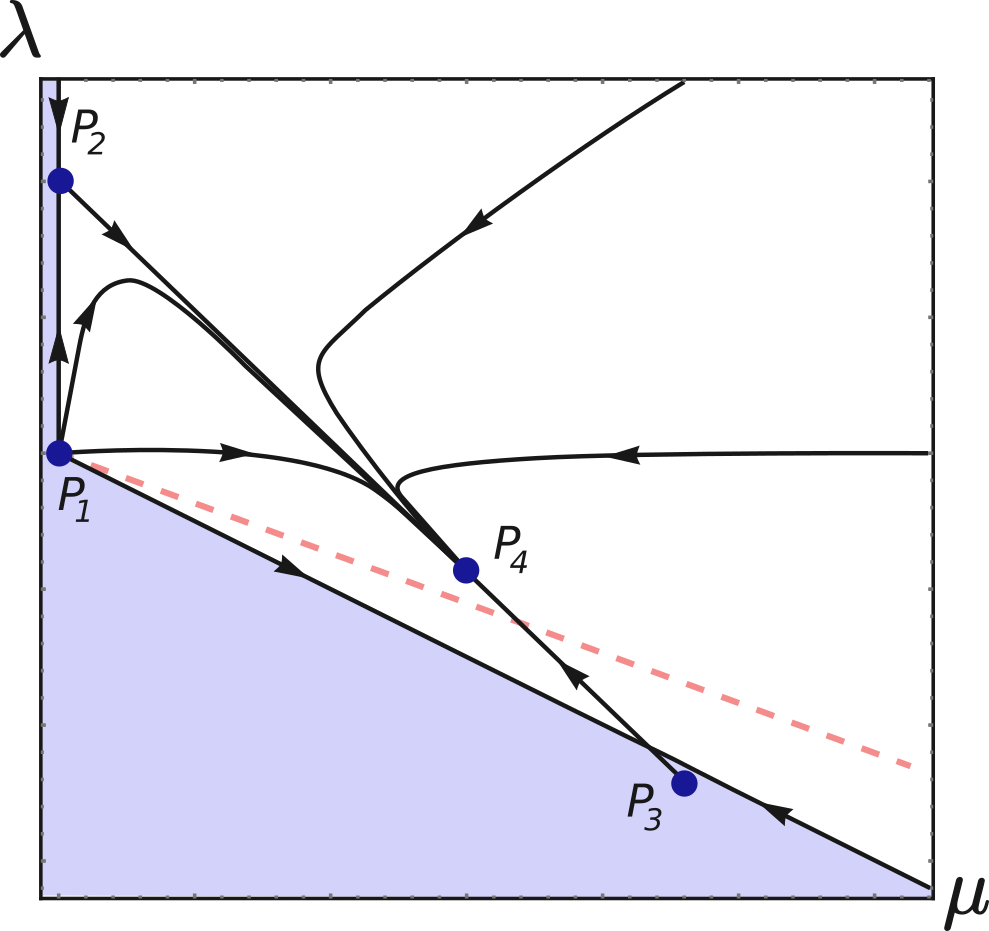
Figure 1: The schematic RG flow diagram (not to scale) on the plane $(\mu,\lambda)$. The stability region of action (1) is delimited by the line $2\lambda+\mu=0$ on which lies the fixed point $P_{3}$ at one-loop order and the line $\mu=0$ on which lies the fixed point $P_{2}$. The dashed line corresponds to the one-loop attractive subspace $3\lambda+\mu=0$ where the stable fixed point $P_{4}$ stands. At two-loop order, $P_{4}$ does not stand exactly on the line $3\lambda+\mu=0$ anymore whereas $P_{3}$ is ejected out the stability region.

II.3.2 Two-loop order

At two-loop order there are still four fixed points. For the two first ones, nothing changes whereas, for the two last ones, the situation changes only marginally:

(i) the Gaussian fixed point $P_{1}$ remains twice unstable.

(ii) The once unstable fixed point $P_{2}$ keeps the same coordinates as at one-loop order – with in particular $\mu_{2}^{*}=0$ – thus the associated anomalous dimension, which is proportional to $\mu$, see (9), still vanishes: $\eta_{2}=O(\epsilon^{3})$.

(iii) At the other once unstable fixed point $P_{3}$, whose coordinates and associated exponent are given in Table 1, the bulk modulus $B$ becomes now slightly negative – and of order $\epsilon^{2}$ – see Fig.1. It follows that, at this order, $P_{3}$ is ejected out of the stability region. However, we emphasize that this fact fully depends on the technique or – two-field or effective – formulation of the theory – see below. It is, thus, likely that this is an artifact of the present computation. So one can still consider $P_{3}$ as potentially present in the genuine flow diagram of membranes.

$\mu^{*}_{3}$	$\displaystyle\frac{96\pi^{2}\,\epsilon}{20+d_{c}}+\frac{80\pi^{2}(-d_{c}+232)}{3(20+d_{c})^{3}}\,\epsilon^{2}$
$\lambda^{*}_{3}$	$\displaystyle\ -\frac{48\pi^{2}\,\epsilon}{20+d_{c}}-\frac{8\pi^{2}(9d_{c}^{2}+265\,d_{c}+2960)}{3(20+d_{c})^{3}}\,\epsilon^{2}$
$\eta_{3}$	$\displaystyle\ \frac{10\,\epsilon}{20+d_{c}}-\frac{d_{c}(37\,d_{c}+950)}{6(20+d_{c})^{3}}\,\epsilon^{2}$

Table 1: Coordinates $\mu^{*}_{3}$ and $\lambda^{*}_{3}$ of the fixed point $P_{3}$ and the corresponding anomalous dimension $\eta_{3}$ at order $\epsilon^{2}$ obtained from the two-field model.

(iv) $P_{4}$ remains fully stable and, thus, still controls the flat phase. Its coordinates and associated anomalous dimension are given in Table 2. As a noticeable point one indicates that this fixed point no longer lies on the line $(D+2)\lambda+2\mu=(6-\epsilon)\lambda+2\mu=0$ – with a distance of order $\epsilon^{2}$ as expected – which is, thus, no longer an attractive line in the infrared.

As can be seen in Table 2 the anomalous dimension at $P_{4}$ is only very slightly modified with respect to its one-loop order value. The extrapolation of our result for $\eta_{4}$ to $D=2$, i.e.  $\epsilon=2$ and $d_{c}=1$ leads, at one and two-loop orders, to $\eta_{4}^{1l}=24/25=0.96$ and $\eta_{4}^{2l}=2856/3125\simeq 0.914$. These values are obviously only indicative and are in no way supposed to provide a quantitatively accurate prediction in $D=2$. However, one can note that the two-loop correction moves the value of $\eta_{4}$ towards the right direction if one refers to the generally accepted numerical data that lie in the range of $[0.72,0.88]$ Guitter et al. (1990); Zhang et al. (1993); M. J. Bowick et. al. (1996); Gompper and Kroll (1997); J. H. Los, M. I. Katsnelson, O. V. Yazyev, K. V. Zakharchenko, and A. Fasolino (2009); A. Tröster (2013); Wein and Wang (2014); A. Tröster (2015); J. H. Los, A. Fasolino and M. I. Katsnelson (2016); A. Kosmrlj and D.R. Nelson (2017); J. Hasik, E. Tosatti and R. Martonak (2018).

$\mu^{*}_{4}$	$\displaystyle\frac{96\pi^{2}\,\epsilon}{24+d_{c}}-\frac{32\pi^{2}(47d_{c}+228)}{5(24+d_{c})^{3}}\,\epsilon^{2}$
$\lambda^{*}_{4}$	$\displaystyle\ -\frac{32\pi^{2}\,\epsilon}{24+d_{c}}+\frac{32\pi^{2}(19d_{c}+156)}{5(24+d_{c})^{3}}\,\epsilon^{2}$
$\eta_{4}$	$\displaystyle\ \frac{12\,\epsilon}{24+d_{c}}-\frac{6d_{c}(d_{c}+29)}{(24+d_{c})^{3}}\,\epsilon^{2}$

Table 2: Coordinates $\mu^{*}_{4}$ and $\lambda^{*}_{4}$ of the flat phase fixed point $P_{4}$ and the corresponding anomalous dimension $\eta_{4}$ at order $\epsilon^{2}$ obtained from the two-field model.

III The flexural mode effective model

III.1 The perturbative approach

We have also considered an alternative approach to the flat phase theory of membranes which is given by the flexural mode effective model (3). There are three main reasons to tackle directly this model. The first one is formal and consists in showing that one can treat, at two-loop order, a model with a nonlocal interaction. The second reason is that this provides a nontrivial check of the previous computations. Indeed the field-content, the (unique) four-point nonlocal vertex as well as the whole structure of the perturbative expansion of the effective model (3) are considerably different from those of the two-field model so that the agreement between the two approaches is a very substantial fact. The last reason to investigate this model is that it involves a new coupling constant $b={\mu\,(D\lambda+2\mu)/(\lambda+2\mu)}$, see (4), which: (i) is directly proportional to the bulk modulus $B$ associated with a stability line of the model and (ii) incorporates a $D$-dependence which, as $b$ is considered as a coupling constant in itself, will be kept from the influence of the dimensional regularization.

III.2 The renormalization group equations

As in the two-field model, one introduces the renormalized field ${\bf h}_{R}$ through $\displaystyle{\bf h}=Z^{1/2}\kappa^{-1/2}{\bf h}_{R}$, the renormalized coupling constants $b_{R}$ and $\mu_{R}$ through

$$\begin{split}&\displaystyle b=k^{\epsilon}Z^{-2}\kappa^{2}Z_{b}\;b_{R}\\ &\mu=k^{\epsilon}Z^{-2}\kappa^{2}Z_{\mu}\;\mu_{R}\end{split}$$ (10)

and the $\beta$-functions $\beta_{b_{R}}=\partial_{t}b_{R}$ and $\beta_{\mu_{R}}=\partial_{t}\mu_{R}$. Using (10) to express the independence of the bare coupling constants $b$ and $\mu$ with respect to $t$ and defining the anomalous dimension

$$\eta=\beta_{b_{R}}\,{\partial\ln Z\over\partial b_{R}}+\beta_{\mu_{R}}\,{\partial\ln Z\over\partial\mu_{R}}$$

the $\beta$-functions $\beta_{b_{R}}$ and $\beta_{\mu_{R}}$ read:

$$\begin{split}&\beta_{b_{R}}\,\partial_{b_{R}}\ln(b_{R}Z_{b})+\beta_{\mu_{R}}\,\partial_{\mu_{R}}\ln(b_{R}Z_{b})=-\epsilon+2\eta\\ \\ &\beta_{b_{R}}\,\partial_{b_{R}}\ln(\mu_{R}Z_{\mu})+\beta_{\mu_{R}}\,\partial_{\mu_{R}}\ln(\mu_{R}Z_{\mu})=-\epsilon+2\eta\ .\end{split}$$

After a rather heavy algebra and using the same techniques as for the two-field model one gets:

$$\begin{split}&\beta_{\mu}=-\epsilon\mu+2\mu\,\eta+\frac{d_{c}\,\mu^{2}}{6(16\pi^{2})}\bigg{(}1+\frac{107b+574\,\mu}{216\,(16\pi^{2})}\bigg{)}\\ \\ &\beta_{b}=-\epsilon b+2b\,\eta\ +\frac{5d_{c}\,b^{2}}{12(16\pi^{2})}\bigg{(}1+\frac{178\,\mu-91b}{216\,(16\pi^{2})}\bigg{)}\end{split}$$ (11)

and:

$$\begin{split}\eta&=\frac{5(b+2\mu)}{6(16\pi^{2})}+\\ &\frac{5\,(15\,d_{c}-212)\,b^{2}+1160\,b\,\mu-4\,(111\,d_{c}-20)\,\mu^{2}}{2592(16\pi^{2})^{2}}\,.\end{split}$$ (12)

III.3 Fixed point analysis

Equations (11) and (12) constitute our second set of results. We now analyze their content.

III.3.1 One-loop order

At one-loop one finds four fixed points:

(i) the Gaussian one $P_{1}$ with $\mu^{*}_{1}=0,\,b^{*}_{1}=0$ and $\,\eta_{1}=0$, which is twice unstable.

(ii) A fixed point, $P_{2}^{\prime}$ with ${\mu}^{\prime*}_{2}=0,\,{b}^{\prime*}_{2}={192\pi^{2}\epsilon/5\,(d_{c}+4)}$ and $\eta_{2}^{\prime}={2\epsilon/(d_{c}+4)}$. This fixed point has no counterpart within the two-field model where $b$ is a function of $\lambda$ and $\mu$ and, in particular, proportional to $\mu$; it is once unstable.

(iii) The infinitely compressible fixed point $P_{3}$ with $\mu^{*}_{3}={96\pi^{2}\epsilon/(d_{c}+20)},\,b^{*}_{3}=0$ and $\eta_{3}=10\,\epsilon/(20+d_{c})$, for which the bulk modulus $B$ vanishes. It thus identifies with the fixed point $P_{3}$ of the two-field model; it is once unstable.

(iv) The fixed point $P_{4}$ with $\mu^{*}_{4}=96\pi^{2}\,\epsilon/(24+d_{c}),b^{*}_{4}={192\pi^{2}\epsilon/5(d_{c}+24)}$ and $\eta_{4}=12\,\epsilon/(24+d_{c})$ which is fully stable and controls the flat phase. It is located on the stable line $5b-2\mu=0$ – corresponding to $(D+1)b-2\mu=0$ in $D$ dimensions – equivalent to the line $3\lambda+\mu=0$ in the two-field model. It fully identifies with the fixed point $P_{4}$ of that model.

Note finally that, as said above, in $D=2$, the tensor $M_{ab,cd}$ vanishes, which is equivalent to the condition $\mu=0$. This implies that the coordinates of the fixed points all obey this condition. As a consequence, in $D=2$, only one nontrivial fixed point, $P_{2}^{\prime}$, remains.

III.3.2 Two-loop order

At two-loop order, as in the two-field model, the one-loop picture is not radically changed.

(i) The Gaussian fixed point $P_{1}$ remains twice unstable.

(ii) At $P_{2}^{\prime}$, ${\mu}^{\prime*}_{2}$ still strictly vanishes whereas ${b}^{\prime*}_{2}$ is only slightly modified, see Table 3. This fixed point, as well as its anomalous dimension $\eta_{2}^{\prime}$ has been first obtained at two-loop order by Mauri and Katsnelson A. Mauri and M.I. Katsnelson (2020) in a very recent study of the Gaussian curvature interaction (CGI) model – see below.

${\mu}^{\prime*}_{2}$	$0$
${b}^{\prime*}_{2}$	$\displaystyle\frac{192\pi^{2}\,\epsilon}{5(4+d_{c})}+\frac{32\pi^{2}(61d_{c}+424)}{75(4+d_{c})^{3}}\,\epsilon^{2}$
$\eta_{2}^{\prime}$	$\displaystyle\frac{2\,\epsilon}{4+d_{c}}+\frac{d_{c}(d_{c}-2)}{6(4+d_{c})^{3}}\,\epsilon^{2}$

Table 3: Coordinates ${\mu}^{\prime*}_{2}$ and ${b}^{\prime*}_{2}$ and the corresponding anomalous dimension $\eta_{2}^{\prime}$ of the fixed point $P_{2}^{\prime}$ at order $\epsilon^{2}$ obtained from the effective model; $P_{2}^{\prime}$ has been first obtained in A. Mauri and M.I. Katsnelson (2020).

(iii) The fixed point $P_{3}$ is interesting as it has a direct counterpart in the two-field model, which allows to study the modifications induced by the change in model. Its coordinates, see Table 4, differ from those of the two-field model, see Table 1, in particular as they still obey the condition $b_{3}^{*}=0$ – or $B=0$ – that puts $P_{3}$ just on the boundary of the stability region of the theory. This fact is an indication that, within the two-loop approach of the two-field model, the location of the fixed point $P_{3}$ out of the stability region is very likely an artifact of the model or of its perturbative approach. This could also be a drawback of the dimensional regularization that seems to mismanage $D$-dependent quantities such as the hypersurface $B=0$. Nevertheless the anomalous dimension $\eta_{3}$, see Table 4, coincides exactly with the two-field result, see Table 1, which is a strong check of our computations.

$\mu^{*}_{3}$	$\displaystyle\frac{96\pi^{2}\,\epsilon}{20+d_{c}}-\frac{80\pi^{2}(13d_{c}+8)}{3(20+d_{c})^{3}}\,\epsilon^{2}$
$b^{*}_{3}$	$0$
$\eta_{3}$	$\displaystyle\frac{10\,\epsilon}{20+d_{c}}-\frac{d_{c}(37d_{c}+950)}{6(20+d_{c})^{3}}\,\epsilon^{2}$

Table 4: Coordinates $\mu^{*}_{3}$ and $b^{*}_{3}$ of the fixed point $P_{3}$ and the corresponding anomalous dimension $\eta_{3}$ at order $\epsilon^{2}$ obtained from the effective model.

(iv) Finally the fixed point $P_{4}$ remains stable and controls the flat phase. Its coordinates and associated exponent $\eta_{4}$ are given in Table 5. In the same way as for the fixed point $P_{3}$, the coordinates of $P_{4}$ at two-loop order differ from those obtained from the two-field model, see Table 2. Also, these coordinates do not obey the condition $(D+1)b^{*}_{4}-2\mu^{*}_{4}=(5-\epsilon)b^{*}_{4}-2\mu^{*}_{4}=0$ corresponding to the one-loop stability line. Nevertheless, again the anomalous dimension $\eta_{4}$ coincides exactly with the two-field model result, see Table 2.

$\mu^{*}_{4}$	$\displaystyle\frac{96\pi^{2}\,\epsilon}{24+d_{c}}-\frac{32\pi^{2}(77d_{c}+948)}{5(24+d_{c})^{3}}\,\epsilon^{2}$
$b^{*}_{4}$	$\displaystyle\frac{192\pi^{2}\,\epsilon}{5(24+d_{c})}+\frac{64\pi^{2}(121d_{c}+3804)}{25(24+d_{c})^{3}}\,\epsilon^{2}$
$\eta_{4}$	$\displaystyle\frac{12\,\epsilon}{24+d_{c}}-\frac{6d_{c}(d_{c}+29)}{(24+d_{c})^{3}}\,\epsilon^{2}$

Table 5: Coordinates $\mu^{*}_{4}$ and $b^{*}_{4}$ of the flat phase fixed point $P_{4}$ and the corresponding anomalous dimension $\eta_{4}$ at order $\epsilon^{2}$ obtained from the effective model.

IV Comparison with previous approaches

We now discuss our results compared to the other techniques – or other models – that have been used to investigate the flat phase of membranes.

SCSA. The SCSA has been studied early Le Doussal and Radzihovsky (1992) to investigate the properties of membranes in any dimension $D$. It is generally employed using the effective action (3) which is more suitable than (1) to establish self-consistent equations. By construction, this approach is one-loop exact. It is also exact at first order in $1/d_{c}$ and, finally, at $d_{c}=0$. Even more remarkably, comparing the anomalous dimensions $\eta_{2}^{\prime}$, $\eta_{3}$ and $\eta_{4}$ obtained in this context to the two-loop results, see Table 6, one observes that the first one is exact at order $\epsilon^{2}$ whereas the latter ones are almost exact at this order as only the coefficients in $\epsilon^{2}/d_{c}^{2}$ differ slightly from those of our exact results.

There are two important features of the SCSA approach that should be underlined. First, the solution with a vanishing bare modulus $b=0$, thus corresponding to the fixed point $P_{3}$, leads to a vanishing long-distance effective modulus $b({\bf q})=0$ P. Le Doussal and L. Radzihovsky (2018), in agreement with our results $b^{*}_{3}=0$. Second, under the conditions fulfilled to reach the scaling behaviour associated with the fixed point $P_{4}$, one observes the asymptotic infrared behaviour Le Doussal and Radzihovsky (1992); P. Le Doussal and L. Radzihovsky (2018):

$${\lambda({\bf q})\over\mu({\bf q})}\underset{{\bf q}\to{\bf 0}}{\sim}-{2\over D+2}$$ (13)

in any dimension $D$ – which is equivalent to the condition $(D+2)\lambda+2\mu=0$ or, equivalently, $(D+1)b-2\mu=0$ discussed above. This property has been proposed to work at all orders of the SCSA and even to be exact Gazit (2009) which leads us to wonder about the genuine location of the fixed point $P_{4}$ found perturbatively at two-loop order that violates condition (13).

We finally recall that, in $D=2$, one gets, at leading order, $\eta_{SCSA}^{D=2,l}=0.821$ Le Doussal and Radzihovsky (1992); P. Le Doussal and L. Radzihovsky (2018) and, at next-to-leading order, $\eta_{SCSA}^{D=2,nl}=0.789$ Gazit (2009) which is inside the range of values given above and close to some of the most recent results obtained by means of numerical computations (see, e.g., A. Tröster (2015) that provides $\eta\simeq 0.79$.).

	Two-loop expansion	SCSA	NPRG
$\eta_{2}^{\prime}$	$\displaystyle\frac{2\,\epsilon}{4+d_{c}}+\frac{d_{c}(d_{c}-2)}{6(4+d_{c})^{3}}\,\epsilon^{2}$	$\displaystyle\frac{2\,\epsilon}{4+d_{c}}+\frac{d_{c}(d_{c}-2)}{6(4+d_{c})^{3}}\,\epsilon^{2}$	$\displaystyle{2\epsilon\over 4+d_{c}}+{d_{c}(10+3d_{c})\over 12(4+d_{c})^{3}}\epsilon^{2}$
$\eta_{3}$	$\displaystyle\ \frac{10\,\epsilon}{20+d_{c}}-\frac{d_{c}(37d_{c}+950)}{6(20+d_{c})^{3}}\,\epsilon^{2}$	$\displaystyle\frac{10\,\epsilon}{20+d_{c}}-\frac{d_{c}(37d_{c}+890)}{6(20+d_{c})^{3}}\,\epsilon^{2}$	$\displaystyle\frac{10\,\epsilon}{20+d_{c}}-\frac{d_{c}(69d_{c}+1430)}{12(20+d_{c})^{3}}\epsilon^{2}$
$\eta_{4}$	$\displaystyle\ \frac{12\,\epsilon}{24+d_{c}}-\frac{6d_{c}(d_{c}+29)}{(24+d_{c})^{3}}\,\epsilon^{2}$	$\displaystyle\frac{12\,\epsilon}{24+d_{c}}-\frac{6d_{c}(d_{c}+30)}{(24+d_{c})^{3}}\,\epsilon^{2}$	$\displaystyle\frac{12\,\epsilon}{24+d_{c}}-\frac{\,d_{c}(11d_{c}+276)}{2(24+d_{c})^{3}}\,\epsilon^{2}$

Table 6: Anomalous dimensions $\eta_{2}^{\prime}$, $\eta_{3}$ and $\eta_{4}$ obtained from the two-loop expansion of either the two-field or the effective model (this paper) – column 1 – from the SCSA Le Doussal and Radzihovsky (1992); P. Le Doussal and L. Radzihovsky (2018) – column 2 – and from the NPRG J.-P. Kownacki and Mouhanna (2009) – column 3. The two-loop value of $\eta_{2}^{\prime}$ has been first obtained by A. Mauri and M.I. Katsnelson (2020).

NPRG. This approach is, as the SCSA, nonperturbative in the dimensional parameter $\epsilon=4-D$. It is based on the use of an exact RG equation that controls the evolution of a modified, running effective action with the running scale Wetterich (1993) (see Bagnuls and Bervillier (2001); Berges et al. (2002); Delamotte et al. (2004); Pawlowski (2007); Rosten (2012); Delamotte (2012) for reviews). Approximations of this equation are needed and consist in truncating the running effective action in powers of the field-derivatives (and, if necessary, of the field itself). They however lead to RG equations that remain nonperturbative both in $\epsilon$ and in $1/d_{c}$. Such a procedure, called derivative expansion, has been validated empirically at order 4 in the derivative of the field Canet et al. (2003); G. De Polsi, I. Balog, M. Tissier and N. Wschebor (2020) and, more recently, up to order 6 I. Balog, H. Chaté, B. Delamotte, M. Marohni and N. Wschebor (2019), since one observes a rapid convergence of the physical quantities with the order in derivative. More formal argument for the convergence of the series – in contrast to the asymptotic nature of the usual, perturbative, series – have also been given in I. Balog, H. Chaté, B. Delamotte, M. Marohni and N. Wschebor (2019). One should have in mind that this approach, although nonperturbative and, as the SCSA, exact in a whole domain of parameters – at leading order in $\epsilon$, in $1/d_{c}$, in the coupling constant controlling the interaction near the lower-critical dimension, at $d_{c}=0$ – is nevertheless not exact and generally misses the next-to-leading order of the perturbative approaches. For instance, reproducing exactly the weak-coupling expansion at two-loop order requires the knowledge of the infinite series in derivatives Papenbrock and Wetterich (1995); Morris and Tighe (1999). Yet, for a given field theory, the ability of the NPRG to reproduce satisfactorily this subleading contribution is a very good indication of its efficiency. The NPRG equations for the flat phase of membranes have been derived at the first order in derivative expansion in J.-P. Kownacki and Mouhanna (2009) and then with help of ansatz involving the full derivative content in F. L. Braghin and N. Hasselmann (2010); N. Hasselmann and F. L. Braghin (2011). We give in Table 6, column 3, the anomalous dimensions obtained within this approach J.-P. Kownacki and Mouhanna (2009) and re-expanded here at second order in $\epsilon$. First, one notes that, as in the SCSA case, the leading order result is exactly reproduced. Then one can observe that the next-to-leading order is also numerically close or very close to those obtained within the two-loop computation.

It is also interesting to mention that, for the SCSA, the coordinates of the fixed point $P_{3}$ obey the condition of vanishing bulk modulus

$$B=O(\epsilon^{3})$$ (14)

whereas those of the fixed point $P_{4}$ obey the identity:

$$(6-\epsilon)\lambda_{4}^{*}+2\mu_{4}^{*}=O(\epsilon^{3})\ .$$ (15)

The properties (14) and (15) are, in fact, true nonperturbatively in $\epsilon$ at least within the first order in the derivative expansion performed in J.-P. Kownacki and Mouhanna (2009) and, again, in agreement with the SCSA result (13).

Finally, one should recall that the result obtained in $D=2$ by means of the NPRG approach J.-P. Kownacki and Mouhanna (2009); Coquand et al. (2020b) $\eta_{NPRG}^{D=2}=0.849(3)$ is also very close to that provided by several numerical approaches (see, e.g., J. H. Los, M. I. Katsnelson, O. V. Yazyev, K. V. Zakharchenko, and A. Fasolino (2009); Wein and Wang (2014); J. Hasik, E. Tosatti and R. Martonak (2018) that lead to $\eta\simeq 0.85$).

GCI model. We conclude by quoting a very recent – and first – two-loop, weak-coupling perturbative approach to membranes that has been performed by Mauri and Katsnelson A. Mauri and M.I. Katsnelson (2020) on a variant of the effective model (3) named Gaussian curvature interaction (GCI) model. It is obtained by generalizing to any dimension $D$ the simplified form of the usual effective model (3), i.e. with $M_{ab,cd}=0$, valid in the particular case $D=2$. As a consequence the authors of A. Mauri and M.I. Katsnelson (2020) get a – unique – nontrivial fixed point which, in our context, is nothing but the fixed point $P_{2}^{\prime}$. One of the main results of their analysis is that the two-loop anomalous dimension $\eta_{2}^{\prime}$ coincides exactly with the corresponding SCSA result, a fact which is also observed in Table 6. Our analysis of the complete theory shows that, for the stable fixed point $P_{4}$, a small discrepancy between the two-loop and the SCSA results occurs.

V Conclusion

We have performed the two-loop, weak coupling analysis of the two models describing the flat phase of polymerized membranes. We have determined the RG equations and the anomalous dimensions at this order. We have identified the fixed points, analyzed their properties and computed the corresponding anomalous dimensions. First, one notes that although the coordinates of the fixed points, as well as several $D$-dependent quantities, vary from one model to the other, the anomalous dimensions at the fixed points are very robust as we get the same values from the two models. This provides a very strong check of our computations. It remains nevertheless to understand more profoundly the interplay between the dimensional regularization used here and these $D$-dependent quantities that are inherent in theories with space-time symmetries, such as the present one. Second, the very good agreement between the anomalous dimensions computed in our paper with those obtained from the SCSA and NPRG approaches is a confirmation of the extreme efficiency of these last methods in the context of the theory of the flat phase of polymerized membranes. As said, these two approaches have in common that they both reproduce exactly – by construction – the leading order of all usual perturbative approaches. This, however, does not explain their singular achievements here which more likely rely on the very nature of the flat phase of membranes itself. This is under investigation.