Tunnel-number-one knot exteriors in $S^{3}$ disjoint from proper power curves

Abstract.

As one of the background papers of the classification project of hyperbolic primitive/Seifert knots in $S^{3}$ whose complete list is given in [BK20], this paper classifies all possible R-R diagrams of two disjoint simple closed curves $R$ and $\beta$ lying in the boundary of a genus two handlebody $H$ up to equivalence such that $\beta$ is a proper power curve and a 2-handle addition $H[R]$ along $R$ embeds in $S^{3}$ so that $H[R]$ is the exterior of a tunnel-number-one knot. As a consequence, if $R$ is a nonseparating simple closed curve on the boundary of a genus two handlebody such that $H[R]$ embeds in $S^{3}$, then there exists a proper power curve disjoint from $R$ if and only if $H[R]$ is the exterior of the unknot, a torus knot, or a tunnel-number-one cable of a torus knot.

The results of this paper will be mainly used in proving the hyperbolicity of P/SF knots and in classifying P/SF knots in once-punctured tori in $S^{3}$, which is one of the types of P/SF knots in [BK20]. Together with these results, the preliminary of this paper which consists of three parts: the three diagrams which are Heegaard diagrams, R-R diagrams, and hybrid diagrams, ‘the Culling Lemma’, and locating waves into an R-R diagrams, will also be used in the classification of hyperbolic primitive/Seifert knots in $S^{3}$.

1. Introduction

In [B90] or an available version [B18], Berge constructed twelve families of knots that admit lens space surgeries. These knots are referred to as the Berge knots and described in terms of double-primitive or primitive/primitive(or simply P/P) curves. A P/P curve $\alpha$ is a simple closed curve lying in a genus two Heegaard surface $\Sigma$ of $S^{3}$ bounding two handlebodies $H$ and $H^{\prime}$ such that $\alpha$ is primitive in both $H$ and $H^{\prime}$, i.e., 2-handle additions $H[\alpha]$ and $H^{\prime}[\alpha]$ along $\alpha$ are solid tori. Then we say that a knot $k$ represented by $\alpha$ is a P/P knot and $(\alpha,\Sigma)$ is a P/P position of $k$. Note that a knot may have more than one P/P position.

For a surface-slope $\gamma$, which is defined to be an isotopy class of $\partial N(k)\cap\Sigma$, where $N(k)$ is a tubular neighborhood of $k$ in $S^{3}$, the knot $k$ represented by $\alpha$ admits lens space Dehn surgery. The Berge conjecture claims that the Berge knots cover all knots in $S^{3}$ admitting lens space Dehn surgeries. Much progress for this conjecture has been made, but it is still unsolved. One result toward this conjecture is that all P/P knots are the Berge knots, which is proved in [B08] or independently in [G13]. This implies that the Berge knots are the complete list of P/P knots.

In [D03], Dean introduced primitive/Seifert(or simply P/SF) knots, which is a natural generalization of P/P knots. A primitive/Seifert curve $\alpha$ is a simple closed curve lying in a genus two Heegaard surface $\Sigma$ of $S^{3}$ bounding two handlebodies $H$ and $H^{\prime}$ such that $\alpha$ is primitive in one handlebody, say, $H^{\prime}$, and $\alpha$ is Seifert in $H$, that is to say, $H^{\prime}[\alpha]$ is a solid torus and $H[\alpha]$ is a Seifert-fibered space. Similarly as in P/P knots, we say that a knot $k$ represented by $\alpha$ is a P/SF knot and $(\alpha,\Sigma)$ is a P/SF position of $k$. Also for a surface-slope $\gamma$, since $k(\gamma)\cong H[\alpha]\cup_{\partial}H^{\prime}[\alpha]$ by Lemma 2.3 of [D03], $\gamma$-Dehn surgery $k(\gamma)$ is either a Seifert-fibered space over $S^{2}$ with at most three exceptional fibers or a Seifert-fibered space over $\mathbb{R}P^{2}$ with at most two exceptional fibers. Note that by [EM92], a connected sum of lens spaces can not arise as a Dehn surgery $k(\gamma)$ for hyperbolic P/SF knots.

P/SF knots are of interest, because knots with Dehn surgeries yielding Seifert-fibered spaces are not well understood. Some examples of P/SF knots are given in [D03], [MM05], and [EM02]. However, as the classification of P/P knots is complete, there is a project to classify all hyperbolic P/SF knots. This project has been worked for years and has recently been achieved. See [BK20] for the complete list of hyperbolic P/SF knots along with the surface-slope of the exceptional surgery on each knot that yields a Seifert-fibered space, and the indexes of each exceptional fiber in the resulting Seifert-fibered space.

The project for the classification of hyperbolic P/SF knot requires various backgrounds. This paper provides one of the background materials. Now we explain the results of this paper. Let $R$ be a nonseparating simple closed curve on the boundary of a genus two handlebody $H$. Suppose that a 2-handle addition $H[R]$ along $R$ embeds in $S^{3}$, i.e., $H[R]$ is an exterior of a knot $k$ in $S^{3}$. Then it follows that $k$ is a tunnel-number-one knot in $S^{3}$ whose tunnel is the cocore of the 2-handle. Suppose $\beta$ is another simple closed curve in $\partial H$ disjoint from $R$ which is a proper power curve. A proper power curve is defined to be a simple closed curve in $\partial H$ such that it is disjoint from an essential separating disk in $H$, does not bound a disk in $H$, and is not primitive in $H$.

The goal of this paper is to classify such curves $R$ and $\beta$ in terms of R-R diagrams. R-R diagrams are one way of describing simple closed curves on the boundary of a genus two handlebody. They are a type of planar diagram related to Heegaard diagrams. They are originally introduced by Osborne and Stevens in [OS77] and developed by Berge. Definition and properties of genus $g$ R-R diagrams are given in Section 2.2. Then the main results of this paper are as follows.

Theorem 1.1.

Suppose $R$ and $\beta$ are disjoint simple closed curves on the boundary of a genus two handlebody $H$ such that $H[R]$ embeds in $S^{3}$ and $\beta$ is a proper power curve. Then $R$ and $\beta$ have an R-R diagram with the form shown either in Figure 1a with $s>1$ or Figure 1b with $m,n>0,s>1$, $\gcd(m,n)=1$ such that the set of parameters $(a,b,m,n,s)$ satisfies the condition (1), (2), or (3) below.

1. $a+b=1$ and, (assuming without loss that $(a,b)$ = $(1,0)$), $sm-un=\delta$ for some $u$ with $0<u<s$, which implies that $H[R]$ is the exterior of an $(n,s)$ torus knot in $S^{3}$.

2. $a,b>0$, $m=1$, and $s(a+b)-u[(a+b)n+b]=\delta$, which implies that $H[R]$ is the exterior of an $((a+b)n+bm,s)$ torus knot in $S^{3}$.

3. $a,b>0$, $n>m>1$, $u=1$, and $ms(a+b)-[(a+b)n+bm]=\delta$, which implies that $H[R]$ is the exterior of an $(ms(a+b)\pm 1,s)$ cable about an $(a+b,m)$ torus knot in $S^{3}$ and a separating essential annulus bounded by two parallel copies of the curve $\beta$ is the cabling annulus in $H[R]$.

Theorem 1.2.

Suppose $R$ is a nonseparating simple closed curve on the boundary of a genus two handlebody such that $H[R]$ embeds in $S^{3}$. Then there exists a proper power curve disjoint from $R$ if and only if $H[R]$ is the exterior of the unknot, a torus knot, or a tunnel-number-one cable of a torus knot.

Figure 1. All possible R-R diagrams of disjoint simple closed curves $R$ and $\beta$ up to equivalence on $H$ such that $H[R]$ embeds in $S^{3}$ and $\beta$ is a proper power curve.

The results of this paper are used in the classification project of hyperbolic P/SF knots in $S^{3}$. Especially, they are essential in proving the hyperbolicity of P/SF knots and in classifying P/SF knots in once-punctured tori in $S^{3}$, which is one of the types of P/SF knots in [BK20]. Briefly speaking for the application, if $k$ has a P/SF position $(\alpha,\Sigma)$ such that $\alpha$ is primitive in $H^{\prime}$ and is Seifert in $H$, then since $\alpha$ is primitive in $H^{\prime}$, there exists a complete set of cutting disks $\{D_{M},D_{R}\}$ of $H^{\prime}$ such that the boundary $M$ of $D_{M}$ intersects $\alpha$ once and the boundary $R$ of $D_{R}$ is disjoint from $\alpha$. This implies that $M$ is a meridional curve of $k$ and $H[R]$ is homeomorphic to the exterior of $k$ in $S^{3}$, and furthermore $k$ is a tunnel-number-one knot such that $R$ is the boundary of a cocore of the 1-handle regular neighborhood of a tunnel. Therefore we can conclude that if $k$ has a P/SF position $(\alpha,\Sigma)$, then there exists a simple closed curve $R$ in the boundary of $H$ such that $H[R]$ embeds in $S^{3}$ as the exterior of a tunnel-number-one knot. Theorem 1.1 indicates that there is a close relationship between such a curve $R$ and the existence of a proper power curve.

Together with the results of this paper, the preliminary of this paper will also be used in the classification project of hyperbolic P/SF knots in $S^{3}$. It consists of three parts: three diagrams that are Heegaard diagrams, R-R diagrams, and hybrid diagrams, locating waves in genus two R-R diagrams, and the Culling Lemma. Since hyperbolic P/SF knots in [BK20] are described in terms of R-R diagrams, Section 2 deals with some basics on the three diagrams. Locating waves in genus two R-R diagrams and the Culling Lemma, which are given in Sections 3 and 4 respectively, are related to find a meridian of a P/SF knot or its exterior $H[R]$, which is one of the steps to find all hyperbolic P/SF knots.

More specifically, Section 2 deals with some basics on the three diagrams. We combine a Heeagaard diagram and a R-R diagram to make a hybrid diagram, and we make use of it to transform an R-R diagram which has underlying Heegaard diagram with a cut vertex into that with no cut vertex. In Section 3 we introduce one of the results of [B20], so-called “Waves provide meridians”, which is originated from [B93], and consider how to locate waves based at a nonspearating simple closed curve $R$ into an R-R diagram of $R$. When an R-R diagram of $R$ such that $H[R]$ embeds in $S^{3}$ is given, the location of a wave into the R-R diagram needs to be understood in order to find a meridian of $H[R]$ which can be obtained by surgery on $R$ along a wave due to the result of [B20]. In Section 4, the “Culling Lemma” is established, which is a tool to cull out meridian candidates of $H[R]$.

Acknowledgement. In 2008, in a week-long series of talks to a seminar in the department of mathematics of the University of Texas as Austin, John Berge outlined a project to completely classify and describe the primitive/Seifert knots in $S^{3}$. The present paper, which provides some of the background materials necessary to carry out the project, is originated from the joint work with John Berge for the project. I should like to express my gratitude to John Berge for his support and collaboration. I would also like to thank Cameron Gordon and John Luecke for their support while I stayed in the University of Texas at Austin.

2. Heegaard diagrams, R-R diagrams, and Hybrid diagrams

In this section we describe some basics on Heegaard diagrams, R-R diagrams, and hybrid diagrams, which will be used in the other sections.

2.1. Heegaard diagrams

First, we deal with the definition and property of Heegaard diagram of simple closed curves lying in the boundary of a genus two handlebody, and some of its terminologies that are needed in this paper.

Suppose $\mathcal{C}$ is a finite set of pairwise disjoint nonparallel simple closed curves in the boundary of a genus two handlebody $H$, none of the curves bound disks in $H$, and $\{D_{A},D_{B}\}$ is a complete set of cutting disks of $H$. Cutting $H$ open along $D_{A}$ and $D_{B}$ cuts $\mathcal{C}$ into set of arcs $E(\mathcal{C})$ and cuts $H$ into a 3 ball $W$. Then $\partial W$ contains disks $D_{A}^{+},D_{A}^{-},D_{B}^{+},$ and $D_{B}^{-}$ such that gluing $D_{A}^{+}$ to $D_{A}^{-}$ and $D_{B}^{+}$ to $D_{B}^{-}$ reconstitutes $\mathcal{C}$ and $H$. Figures 2 and 3 illustrate this process.

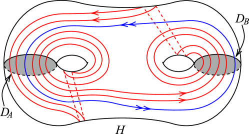
Figure 2. Two simple closed curves in the boundary of a genus two handlebody.

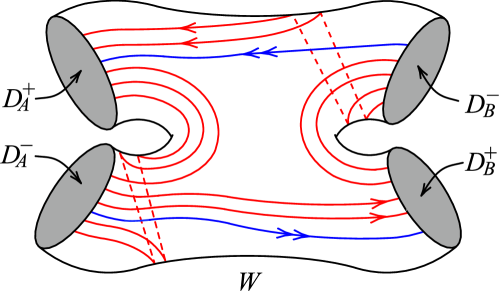
Figure 3. A 3-ball $W$ obtained by cutting $H$ open along $D_{A}$ and $D_{B}$.

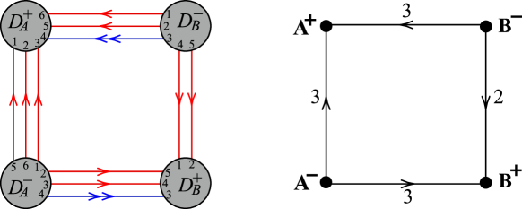
Figure 4. Heegaard diagram and its underlying graph.

The set of arcs $E(\mathcal{C})$ forms the edges of Heegaard diagrams in $\partial W$ with “fat”, i.e., disk rather than point, vertices $D_{A}^{+},D_{A}^{-},D_{B}^{+},$ and $D_{B}^{-}$. If one ignores how $D_{A}^{+}$ and $D_{B}^{+}$ are identified with $D_{A}^{-}$ and $D_{B}^{-}$ to reconstitute $H$, the set of arcs $E(\mathcal{C})$ also forms the edges of a graph in $\partial W$ with vertices $D_{A}^{+},D_{A}^{-},D_{B}^{+},$ and $D_{B}^{-}$. Let $G$ denote the graph in $\partial W$ whose edges are the arcs in $E(\mathcal{C})$. Then $G$ is the graph underlying the Heegaard diagram of $\mathcal{C}$. Some simplification can be made. If there are $n$ parallel edges in $G$, then we merge these parallel edges into one and recode this edge by placing the integer $n$ near the edge. Also we smash the disks $D_{A}^{+},D_{B}^{-},D_{B}^{+},$ and $D_{B}^{-}$ in $\partial W$ into points denoted by $A^{+},A^{-},B^{+},$ and $B^{-}$. Figure 4 shows the Heegaard diagram and the underlying graph of the curves $k_{1}$ and $k_{2}$ in Figure 2. Note that this graph is not just abstract graph, since it inherits specific embeddings in the 2-sphere $S^{2}$ which is homeomorphic to $\partial W$ from the Heegaard diagram which it underlie.

The following lemma, which can be found in [HOT80] or [O79], shows some possible types of graphs of Heegaard diagrams of simple closed curves on the boundary of a genus two handlebody.

Figure 5. The three types of graphs of Heegaard diagrams of simple closed curves on the boundary of a genus two handlebody $H$ which has cutting disks $D_{A}$ and $D_{B}$, excluding diagrams in which simple closed curves are disjoint from both $\partial D_{A}$ and $\partial D_{B}$.

Lemma 2.1.

Let $H$ be a genus two handlebody with a set of cutting disks $\{D_{A},D_{B}\}$ and let $\mathcal{C}$ be a finite set of pairwise disjoint nonparallel simple closed curves on $\partial H$ whose intersections with $\{D_{A},D_{B}\}$ are essential and not both empty. Then, after perhaps relabeling $D_{A}$ and $D_{B}$, the Heegaard diagram of $\mathcal{C}$ with respect to $\{D_{A},D_{B}\}$ has the form of one of the three graphs in Figure 5.

Definition 2.2 (Complexity).

The complexity of a Heegaard diagram—without simple closed curve components—is the total number of edges of the diagram. The complexity is denoted by $|\mathcal{C}|$.

Definition 2.3 (cut-vertex).

If $v$ is a vertex of a connected graph $G$ such that deleting $v$ and the edges of $G$ meeting $v$ from $G$ disconnects $G$, we say $v$ is a cut-vertex of $G$.

The complexity of the Heegaard diagrams in Figure 5 is $2a+2b+c+d$, and the Heegaard diagram in Figure 5c either is not connected or has a cut-vertex.

Definition 2.4 (Positive Heegaard Diagram).

A Heegaard diagram is positive if the curves of the diagram can be oriented so that all intersections of curves in the diagram are positive. Otherwise, the diagram is nonpositive.

See Figures 17 and 19 for examples of a nonpositive diagram and a positive diagram respectively.

2.2. R-R diagrams

In this subsection we describe the definition of an R-R diagram and its basic properties. R-R diagrams are a type of planar diagram related to Heegaard diagrams. These diagrams were originally introduced by Osborne and Stevens in [OS77] and developed by Berge. They are particularly useful for describing embeddings of simple closed curves in the boundary of a handlebody so that the embedded curves represent certain conjugacy classes in $\pi_{1}$ of the handlebody. In addition, R-R diagrams are much easier to parametrize and to see structural details of systems of curves than standard Heegaard diagrams.

2.2.1. Genus $g$ R-R diagrams

We provide the basics of genus $g$ R-R diagrams describing curves lying in the boundary of a genus $g$ surface.

Consider the following construction of a closed orientable surface $\Sigma_{g}$ of genus $g$. Start with a planar surface $S_{g}$ with $g$ boundary components $\beta_{i}$ and $g$ handles $F_{i}$, $1\leq i\leq g$, each of which is a once-punctured torus. Then cap off each boundary component of $S_{g}$ by identifying $\partial F_{i}$ with $\beta_{i}$. The resulting surface $\Sigma_{g}$ is naturally endowed with a set of $g$ pairwise disjoint separating simple closed curves $\beta_{i}$ for $1\leq i\leq g$, each of which is the boundary of a corresponding handle $F_{i}$.

Now suppose $\mathcal{C}$ is a finite collection of pairwise disjoint simple closed curves in $\Sigma_{g}$. The decomposition of $\Sigma_{g}$ into a planar component $S_{g}$ and a set of $g$ handles by the separating curves $\beta_{i}$, $1\leq i\leq g$, gives $\Sigma_{g}$ a structure which can be used to study sets of simple closed curves, such as $\mathcal{C}$, on $\Sigma_{g}$. Zieschang does this in several places; see e.g. the expository paper [Z88] or [Z62], [Z63a], [Z63b]. In Zieschang’s terminology, the $\beta_{i}$s are belt curves. It is usually convenient to assume that the number of intersections of the curves in $\mathcal{C}$ with the members of the set of belt curves $\beta_{i}$ has been minimized by isotopies in $\Sigma_{g}$. Then a curve $C$ in $\mathcal{C}$ either lies completely in $S_{g}$, or entirely on one of the $g$ handles $F_{i}$, or $C$ is cut by its intersections with the belt curves $\beta_{i}$ into arcs, each either properly embedded and essential in $S_{g}$, or properly embedded and essential in some handle $F_{i}$.

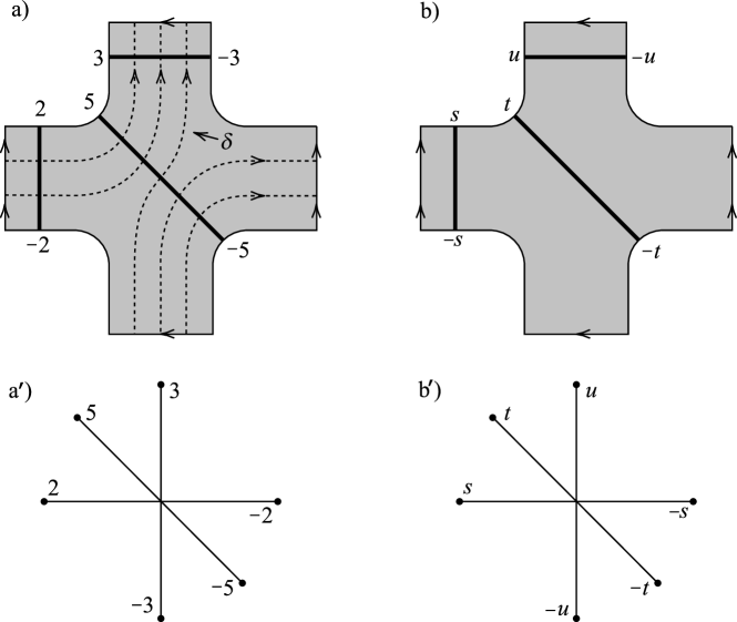
Figure 6. Punctured tori handles.

A properly embedded essential arc in a handle $F_{i}$ is a connection. Two connections on $F_{i}$ are parallel if they are isotopic via an isotopy which keeps their endpoints in $\partial F_{i}$. A collection of pairwise disjoint connections on a given handle can be partitioned into bands of pairwise parallel connections. Then it is easy to see that, on a once-punctured torus, there can be at most three nonparallel bands of connections. Figure 6a or 6b illustrates this situation, where the shaded region of Figure 6a or 6b is an octagon obtained by cutting a punctured torus handle $F$ open along two nonparallel properly embedded essential arcs. This leaves the four edges of the octagon marked with arrows, which must be identified in pairs to recover the punctured torus.

Note that sets of pairwise nonparallel connections in a once-punctured torus are unique up to homeomorphism. In particular, if $F$ is a once-punctured torus, $\Delta=\{\alpha_{1},\ldots,\alpha_{i}\},1\leq i\leq 3$ is a set of pairwise nonparallel connections in $F$, and $\Delta^{\prime}=\{\alpha^{\prime}_{1},\ldots,\alpha^{\prime}_{j}\},1\leq j\leq 3$ is another set of pairwise nonparallel connections in $F$, and $i=j$, then there is a homeomorphism of $F$ which takes $\Delta$ to $\Delta^{\prime}$.

Some simplifications can be made at this point without losing any information about the embedding of the curves of $\mathcal{C}$ in $\Sigma_{g}$. Suppose $F$ is a handle, and let $\mathcal{C}_{S_{g}}$ be the set of arcs in which curves of $\mathcal{C}$ intersect $S_{g}$. Then each set of parallel connections on $F$ can be merged into a single connection. (This also merges some endpoints of arcs in $\mathcal{C}_{S_{g}}$ meeting $\partial F$.)

After such mergers, $F$ carries at most 3 pairwise nonparallel connections. Continuing, after each set of parallel connections on $F$ has been merged, additional mergers of sets of properly embedded parallel subarcs of $\mathcal{C}_{S_{g}}$ can also be made; although now whenever, say, $n$ parallel arcs merged into one, this needs to be recorded by placing the integer $n$, which is called a weight, near the single arc resulting from the merger.

Merging parallel connections in each handle turns the set of pairwise disjoint simple closed curves in $\mathcal{C}$ into a graph $\mathcal{G}$ in $\Sigma_{g}$ whose vertices are the endpoints of the remaining connections in each handle. Clearly $\mathcal{G}$ and its embedding in $\Sigma_{g}$ completely encodes the embedding of the curves of $\mathcal{C}$ in $\Sigma_{g}$.

A problem with $\mathcal{G}$ is that in general it is not planar. However, $\mathcal{G}$ always has a nice immersion $I(\mathcal{G})$ in the plane $\mathbb{R}^{2}$, which becomes an R-R diagram of the curves of $\mathcal{C}$ in $\Sigma_{g}$.

To produce $I(\mathcal{G})$, first remove a small disk $D$, disjoint from $\mathcal{G}$, from the interior of $S_{g}$. Then embed $S_{g}-D$ in $\mathbb{R}^{2}$ so that each handle $F$ bound disjoint round disks, say $\mathcal{F}$ in $\mathbb{R}^{2}$.

Next, note that if $\alpha$ and $\alpha^{\prime}$ are nonparallel connections on a handle $F$, the endpoints of $\alpha$ separate the endpoints of $\alpha^{\prime}$ in the belt curve $\partial F$. It follows that, if $u$ and $v$ in $\partial F$ are the endpoints of a connection $\alpha$ in $\partial F$, we may assume that $u$ and $v$ bound a diameter $d_{\alpha}$ in $\mathcal{F}$. This results in each round disk $\mathcal{F}$ containing $0,1,2,$ or $3$ diameters passing through its center, with each diameter an image of a connection in $F$, where the number of such diameters depends upon whether $F$ originally contained respectively $0,1,2,$ or $3$ bands of parallel connections. Figure 6 shows 3 connections and thus 3 diameters.

Now we encode the endpoints of each diameter, i.e., endpoints of each connection in $F$. Representatives of three types of connections on $F$ are shown in bold in Figure 6a, along with a nonseparating simple closed curve $\delta$ lying in the interior of $F$, which appears as the “dotted” curve in Figure 6a. Then the integer labels at the ends of the three bands of connections in Figure 6a give signed intersection numbers of any oriented connections lying in the three illustrated bands of connections in $F$ with $\delta$.

Figure 6b again shows $F$, but the set of integers, which labeled the ends of the bands of connections in Figure 6a, has been replaced with a set of integer parameters $\{s,t,u,-s,-t,-u\}$, which appear in clockwise cyclic order $(s,t,u,-s,-t,-u)$ around the boundary $\beta$ of $F$, and the curve $\delta$ has disappeared. Figures 6a^′ and 6b^′ illustrate the labels of the endpoints of corresponding diameters in $F$. A connection whose endpoints are labeled by $x$ and $-x$ is simply said to be $x$-connection or $-x$-connection.

Now the well-known characterization of the homology classes in $H_{1}(F;\mathbb{Z})$ which can be represented by simple closed curves implies the following proposition.

Proposition 2.5.

There exists a nonseparating simple closed curve $\delta$ in $F$ such that $\delta$ has the algebraic intersection numbers shown in Figure 6b with oriented connections in the bands of connections of Figure 6b if and only if $\gcd(s,u)=1$ and $t=s+u$. Furthermore, the isotopy class of $\delta$ in $F$ is uniquely determined by the algebraic intersection numbers of any two nonparallel bands of connections in $F$.

Note that if there are two or three bands of connections in $F$ and if the absolute value of one of labels of endpoints of the bands of connections is greater than $2$, then the labels determine the connections up to a homeomorphism of $F$ which is the identity on $\partial F$. If all the labels have absolute value $1$ and $2$, or $1$ only, the labels do not determine the connections in $F$. Furthermore, if there is only one band of connections with label $s>0$, there are $\phi(s)$ inequivalent connections with the same label $s$, where $\phi(s)$ is the number of positive integers $s^{\prime}$ such that gcd$(s,s^{\prime})=1$. This is what we want to generalize in the following way.

A generalization occurs when the punctured torus $F$ has been endowed with a pair of embedded oriented simple closed curves, say, $\vec{m}$ and $\vec{l}$, which meet transversely at a single point and form a basis for $H_{1}(F)$. Then each band of connections on $F$ can be labeled with an ordered pair of integers which represent the coordinates of an oriented connection in that band with respect to the basis formed by $\vec{m}$ and $\vec{l}$. This ordered pair of integers characterizes the connection up to a homeomorphism of $F$. Furthermore if there are the pairs of labels on distinct bands, then they must satisfy a unimodular determinant condition. That is, if two distinct bands of connections have labels of the form $(s,s^{\prime})$ and $(u,u^{\prime})$, then $su^{\prime}-us^{\prime}=\pm 1$. Proposition 2.6 and Figure 7 illustrate the situation.

Proposition 2.6.

Suppose $\alpha$ and $\beta$ are simple closed curves with an R-R diagram of the form shown in Figure 7a. If the diagram of Figure 7a is interpreted as describing embeddings of $\alpha$ and $\beta$ in the punctured torus $T$ shown in Figure 7b so that $[\vec{\alpha}]=s[\vec{l}\>]+s^{\prime}[\vec{m}]$ and $[\vec{\beta}\,]=u[\vec{l}\>]+u^{\prime}[\vec{m}]$ in $H_{1}(F)$, then $su^{\prime}-us^{\prime}=1$.

Proof.

If $\alpha$ and $\beta$ embed in $T$ with $\alpha\cap\beta$ a single point of transverse intersection, as shown in Figure 7a, then there is an orientation preserving homeomorphism $\theta$ of $F$ such that $\theta(\vec{l}\>)=\vec{\alpha}$ and $\theta(\vec{m})=\vec{\beta}$. If $[\vec{\alpha}]=s[\vec{l}\>]+s^{\prime}[\vec{m}]$ and $[\vec{\beta}\,]=u[\vec{l}\>]+u^{\prime}[\vec{m}]$ in $H_{1}(F)$, then $\theta$ induces an automorphism of $H_{1}(F)$ whose determinant is equal to $su^{\prime}-us^{\prime}$, which must be plus one, since $\theta$ is orientation-preserving. ∎

Figure 7. A pair of figures, used to show that labels $(s,s^{\prime})$ and $(u,u^{\prime})$ of connections on a handle $B$ of an R-R diagram, as shown in Figure 7a, must satisfy $su^{\prime}-s^{\prime}u=1$, if $[\vec{\alpha}]=s[\vec{l}]+s^{\prime}[\vec{m}]$ and $[\vec{\beta}]=u[\vec{l}]+u^{\prime}[\vec{m}]$ in $H_{1}$ of the punctured torus in Figure 7b.

One practical example of this generalization can be made when we consider knots lying in a genus $g$ Heegaard surface $\Sigma_{g}$ of $S^{3}$ which is standardly embedded and bounds two handlebodies $H$ and $H^{\prime}$ in $S^{3}$. As constructed at the beginning, suppose $\Sigma_{g}$ is obtained from a planar surface $S_{g}$ with $g$ boundary components $\beta_{i}$ by gluing $g$ handles $F_{i}$ along $\beta_{i}$, $1\leq i\leq g$. Also suppose for each $i$, $D_{A_{i}}$ and $D_{A^{\prime}_{i}}$ are cutting disks of $H$ and $H^{\prime}$ respectively such that $\partial D_{A_{i}}$ and $\partial D_{A^{\prime}_{i}}$ lie in a handle $F_{i}$ and intersect transversely at a point. Then the two curves $\partial D_{A_{i}}$ and $\partial D_{A^{\prime}_{i}}$ give the labelling of one end of a band of connections by $(s,s^{\prime})$ in $F_{i}$. The R-R diagram that is constructed in this way provides an embedding of simple closed curves(or knots) lying in a Heegaard surface of $S^{3}$ which is standardly embedded in $S^{3}$. Thus we make the following terminology.

Definition 2.7 (GDS R-R diagram).

Let $\Sigma_{g}$ be a genus $g$ Heegaard surface of $S^{3}$ bounding two handlebodies $H$ and $H^{\prime}$ and $\mathcal{C}$ be the set of pairwise disjoint simple closed curves in $\Sigma_{g}$. Suppose $\Sigma_{g}$ is obtained from a planar surface $S_{g}$ with $g$ boundary components $\beta_{i}$ by gluing $g$ handles $F_{i}$ along $\beta_{i}$, $1\leq i\leq g$. Suppose $\mathfrak{D}=\{D_{A_{1}},\ldots,D_{A_{g}}\}$ and $\mathfrak{D}^{\prime}=\{D_{A^{\prime}_{1}},\ldots,D_{A^{\prime}_{g}}\}$ are complete sets of cutting disks of $H$ and $H^{\prime}$ respectively such that $\partial D_{A_{i}}$ and $\partial D_{A^{\prime}_{i}}$, $1\leq i\leq g$, lie in a handle $F_{i}$ and intersect transversely at a point. Then the R-R diagram of $\mathcal{C}$ on $\Sigma_{g}$ with respect to $\mathfrak{D}$ and $\mathfrak{D}^{\prime}$ is said to be a great disk system of R-R diagram of $\mathcal{C}$, or simply GDS R-R diagram of $\mathcal{C}$. Also each handle $F_{i}$ in the R-R diagram is said to be an $(A_{i},A^{\prime}_{i})$-handle.

One example of an R-R diagram and a GDS R-R diagram will be given in the next subsection.

2.2.2. Genus two R-R diagrams

Since we are interested in curves in the boundary of a genus two handlebody, as a special case, this subsection shows how to make a geuns two R-R diagram, or simply R-R diagram of, for example, two curves $k_{1}$ and $k_{2}$ in Figure 2. We follow the procedure given in the previous subsection. Note that the basics of genus two R-R diagrams were also given in [B09] and an example of genus two R-R diagrams was given in [K14], which we will use here as a same example.

By considering two parallel separating curves, i.e., belt curves as shown in Figure 8, we decompose the boundary of $H$ into two handles $F_{A}$, $F_{B}$, and one annulus $\mathcal{A}$, so that the two handles $F_{A}$ and $F_{B}$ contain $\partial D_{A}$ and $\partial D_{B}$ respectively, which can be considered as a nonseparating curve $\delta$ in each handle. Figure 9 shows this decomposition.

Note from Figure 9 that there are three nonparallel bands of connections in $F_{A}$, each of which consists of one connection, and there are two nonparallel bands of connections in $F_{B}$, one of which contains one connection and the other contains two. Therefore there are three diameters in $\mathcal{F}_{A}$ and two in $\mathcal{F}_{B}$ as shown in Figure 11.

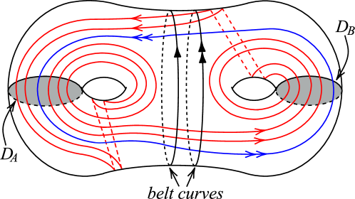
Figure 8. Belt curves bounding an annulus in a genus two surface.

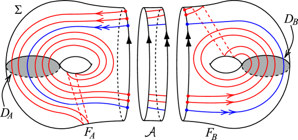
Figure 9. An annulus $\mathcal{A}$ and two handles $F_{A}$ and $F_{B}$.

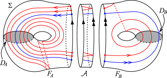
Figure 10. Merging the parallel connections and the endpoints of the arcs in the annulus $\mathcal{A}$.

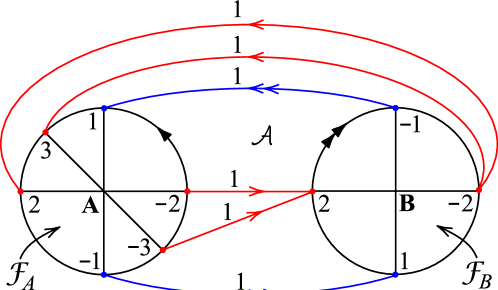
Figure 11. Immersion of curves of $\mathcal{C}$ into $S^{2}$ which becomes an corresponding R-R diagram.

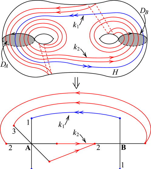
Figure 12. Transformation into R-R diagram.

Merging the parallel connections and thus the endpoints of the connections leads to mergers of the endpoints of arcs in the annulus $\mathcal{A}$ as in Figure 10. We observe from Figure 10 that after this merger, no pair of the arcs in $\mathcal{A}$ have the same endpoints and thus each arc has label $1$.

In order to put the labels of the endpoints of each diameter (or each band of connections), we take the $\partial D_{A}$ and $\partial D_{B}$ in $F_{A}$ and $F_{B}$ respectively as a nonseparating curve $\delta$ in a handle. Then the integer parameters $s,t,u$ of the diameters on $F_{A}$(or $F_{B}$) imply the intersection numbers with the cutting disk $D_{A}$(or $D_{B}$). The labels of each diameter are given in Figure 11.

With all of the information obtained, we can make an immersion of $k_{1}$ and $k_{2}$ into $S^{2}$ which becomes a corresponding R-R diagram. First embed the annulus $\mathcal{A}$ in $S^{2}$ obtained by deleting two disks from $S^{2}$ whose boundaries correspond to $\partial F_{A}$ and $\partial F_{B}$ as shown in Figure 11. We put the capital letters A and B to indicate correspondence to the two handles $F_{A}$ and $F_{B}$ respectively and we call the corresponding handles as $A$-handle and $B$-handle. Last, we disregard the boundary circles of $F_{A}$ and $F_{B}$ in Figure 11 and one of the labels of the endpoints of each band of connections to obtain the corresponding R-R diagram. Figure 12 shows the curves $k_{1}$ and $k_{2}$ in $\partial H$ and the corresponding R-R diagram.

Since a complete set of cutting disks $\{D_{A},D_{B}\}$ of $H$ is used in the construction of an R-R diagram, there is a Heegaard diagram underlying the R-R diagram, which is obtained by cutting $H$ open along the cutting disks $D_{A}$ and $D_{B}$.

R-R diagrams give sufficient information about conjugacy classes of the element represented by a simple closed curve $k$ in $\pi_{1}(H)$. $\pi_{1}(H)$ is a free group $F(A,B)$ which is generated by $A$ and $B$ dual to the cutting disks $D_{A}$ and $D_{B}$ respectively. It follows from Figure 12 that $k_{1}$ and $k_{2}$ represent the conjugacy classes of $AB$ and $A^{3}B^{2}A^{2}B^{2}$ respectively in $\pi_{1}(H)$.

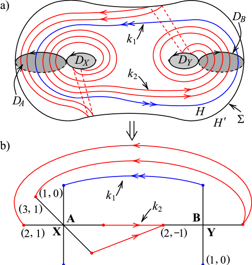
Figure 13. Two simple closed curves $k_{1}$ and $k_{2}$ lying in a standard genus two Heegaard splitting $(\Sigma,H,H^{\prime})$ of $S^{3}$ and their GDS R-R diagrams.

If we consider the handlebody $H$ to be embedded standardly in $S^{3}$ as in Figure 13a so that the complement of $H$ is another handlebody $H^{\prime}$ with a complete set of cutting disks $\{D_{X},D_{Y}\}$ and $\Sigma$ is the common boundary of $H$ and $H^{\prime}$. Figure 13b shows a GDS R-R diagram of $k_{1}$ and $k_{2}$ with respect to the Heegaard splitting $(\Sigma;H,H^{\prime})$ with complete sets of cutting disks $\{D_{A},D_{B}\}$ and $\{D_{X},D_{Y}\}$. Note that $k_{1}$ has $(1,0)$-connections in both $A$- and $B$-handles, and $k_{2}$ has $(3,1)$- and $(2,1)$-connection in the $(A,X)$-handle, and $(2,-1)$-connection in the $(B,Y)$-handle. We see that the labels of the connections satisfy the unimodular determinant condition in Proposition 2.6.

Now we finish this subsection by defining the equivalence of R-R diagrams.

Definition 2.8 (Equivalent R-R diagrams).

Let $k$ and $k^{\prime}$ be two simple closed curves on the boundary of a genus two handlebody $H$. Let $\mathcal{D}_{k}(\mathcal{D}_{k^{\prime}},\textrm{resp}.)$ be an R-R diagram of $k(k^{\prime},\textrm{resp}.)$ underlying a Heegaard diagram $\mathbb{D}_{k}(\mathbb{D}_{k^{\prime}},\textrm{resp}.)$ of $k(k^{\prime},$ $\textrm{resp}.)$ with respect to a complete set of cutting disks $\{D_{A},D_{B}\}(\{D_{A^{\prime}},D_{B^{\prime}}\},\textrm{resp})$.

Then $\mathcal{D}_{k}$ is equivalent to $\mathcal{D}_{k^{\prime}}$ if there is a homeomorphism of $H$ onto itself sending $\{D_{A},D_{B}\}$ to $\{D_{A^{\prime}},D_{B^{\prime}}\}$ and sending $k$ to $k^{\prime}$.

2.3. Hybrid diagrams

In this section, we will explain the definition of hybrid diagrams (of genus two) and its basic properties. Hybrid diagrams are a type of planar graph which is a combination of Heegaard diagrams and R-R diagrams.

Some R-R diagrams of simple closed curves might be needed to transform into other R-R diagrams to apply for appropriate theories related to R-R diagrams. For example, some R-R diagrams might have underlying Heegaard diagrams with a cut-vertex, which happen when all of the labels of connections in one handle are $0$ or $1$. In this case we have some difficulty in using theories such as surgery of a curve along a wave described in Theorem 3.1, which can only be applied to Heegaard diagrams with no cut-vertex. Therefore we need to transform R-R diagram into that which overlies a Heegaard diagram with no cut-vertex. This transformation can be achieved by a change of cutting disks of a genus two handlebody $H$ which induces an automorphism on the free group of $\pi_{1}(H)$. Then hybrid diagrams are useful to perform such a change of cutting disks.

To define hybrid diagrams, we start with an R-R diagram of a simple closed curve $k$. By the construction of R-R diagram from a genus two handlebody $H$ with a complete set of cutting disks $\{D_{A},D_{B}\}$, there is a separating curve $\beta$ (one of the belt curves) in $\partial H$ splitting $\partial H$ into two handles $F_{A}$ and $F_{B}$ such that $F_{A}$ ($F_{B}$, respectively) contains $\partial D_{A}$ ($\partial D_{B}$, respectively). Now we consider the Heegaard diagram underlying the R-R diagram, which is obtained by cutting $H$ open along the cutting disks $D_{A}$ and $D_{B}$. The separating curve $\beta$ also separates this diagram into two parts $F^{\prime}_{A}$ and $F^{\prime}_{B}$ such that $F^{\prime}_{A}$ ($F^{\prime}_{B}$, respectively) contains $\partial D_{A}$ ($\partial D_{B}$, respectively). Figures 14a and 14b show an example of R-R diagram of a simple closed curve $k$ and its underlying Heegaard diagram with the separating curve $\beta$ in each of the diagrams. Here, we assume that $S,T>0$ and $|S-T|>1$ in Figure 14a. Note that since the labels of the endpoints of the bands of connections in the $A$-handle are only $0$ or $1$, the underlying Heegaard diagram has a cut-vertex.

To get a Heegaard diagram without no cut-vertex, we need to perform a change of cutting disks as follows. First, replace one of two handles, say, the $A$-handle corresponding to $F_{A}$ in the R-R diagram by $F^{\prime}_{A}$ in the Heegaard diagram. In the example of the R-R diagram in Figure 14a, since a cut-vertex arises due to the $A$-handle where there are only $0$ and $1$-connections, we ought to replace the $A$-handle in order to obtain a Heegaard diagram with no cut-vertex. The resulting diagram is shown in Figure 15a and is called a hybrid diagram.

Figure 14. An R-R diagram and its underlying Heegaard diagram which has a cut-vertex.

Using a hybrid diagram, we can perform a change of cutting disks of a genus two handlebody $H$ with a complete set of cutting disks $\{D_{A},D_{B}\}$ to obtain a new R-R diagram. Suppose, for example, a simple closed curve $k$ has a hybrid diagram of the form shown in Figure 15a. Now we drag the vertex $A^{-}$ together with the edges of $k$ over the $S$-connection on the $B$-handle. This performance corresponds to a change of cutting disks inducing an automorphism of $\pi_{1}(H)$ which takes $A\mapsto AB^{-S}$ and leaves $B$ fixed. In other words, with the cutting disk $D_{A}$ fixed, we change the cutting disk $D_{B}$ into the cutting disk $D_{B^{\prime}}$ which is obtained by bandsumming $D_{B}$ with $D_{A}$ along the arcs of $k$ $S$ times. This induces an automorphism of $\pi_{1}(H)$ which takes $A\mapsto AB^{-S}$ and leaves $B$ fixed. Then the resulting hybrid diagram is shown in Figure 15b, where the $B$-handle has only one connection labeled by $T-S$. Retrieving the $A$-handle from the resulting hybrid diagram, i.e., the number of bands of connections in the $A$-handle depends on how the two copies $A^{+}$ and $A^{-}$ are identified. However, since there are $b+c$ edges connecting the vertices $A^{+}$ and $A^{-}$, the $A$-handle has a band of connection whose label is greater than 1 in the resulting R-R diagram, which implies that the underlying Heegaard diagram has no cut-vertex.

Figure 15. Change of cutting disks of a genus two handlebody using a hybrid diagram inducing an automorphism of $\pi_{1}(H)$ which takes $A\mapsto AB^{-S}$ and leaves $B$ fixed.

3. Locating waves in genus two R-R diagrams

Suppose $R$ is a nonseparating simple closed curve on the boundary of a genus two handlebody $H$ such that $H[R]$ embeds in $S^{3}$, i.e., $H[R]$ is an exterior of a knot $k$ in $S^{3}$. It is shown in [B20] that a meridian of $H[R]$ (or $k$) can be obtained from $R$ by surgery along a wave based at $R$. Recall that a wave on the curve $R$ in $\partial H$ is an arc $\omega$ whose endpoints lies on $R$ with the opposite signs. The following is one of the results of [B20], which shows how to get a meridian of $H[R]$.

Theorem 3.1 (Waves provide meridians).

Let $H$ be a genus two handlebody with a set of cutting disks $\{D_{A},D_{B}\}$ and let $R$ be a nonseparating simple closed curve on $\partial H$ such that the Heegaard diagram $\mathbb{D}_{R}$ of $R$ with respect to $\{D_{A},D_{B}\}$ is connected and has no cut-vertex. Suppose, in addition, that the manifold $H[R]$ embeds in $S^{3}$. Then $\mathbb{D}_{R}$ determines a wave $\omega$, based at $R$, such that if $m$ is a boundary component of a regular neighborhood of $R\cup\omega$ in $\partial H$, with $m$ chosen so that it is not isotopic to $R$, then $m$ represents the meridian of $H[R]$. Furthermore, the wave $\omega$ determined by $R$ can be obtained as follows:

1. If $\mathbb{D}_{R}$ is nonpositive, then $\omega$ is a vertical wave $\omega_{v}$ which is isotopic to a subarc of the boundary of one of $D_{A}$ and $D_{B}$ with which $R$ has both positive and negative signed intersections.

2. If $\mathbb{D}_{R}$ is positive, then $\omega$ is a horizontal wave $\omega_{h}$ such that one endpoint of $\omega_{h}$ lies on an edge of $\mathbb{D}_{R}$ connecting vertices $A^{+}$ and $A^{-}$, while the other endpoint of $\omega_{h}$ lies on an edge of $\mathbb{D}_{R}$ connecting vertices $B^{+}$ and $B^{-}$.

Figure 16. A vertical wave $\omega_{v}$ in a nonpositive Heegaard diagram in a) and b) where $R$ has both positive and negative signed intersections with $D_{B}$, and a horizontal wave $\omega_{h}$ in a positive Heegaard diagram in c). They are said to be distinguished in the sense that they can be used in a surgery on $R$ to obtain a meridian of $H[R]$.

Figures 16a and 16b show vertical waves $\omega_{v}$ when $R$ has both positive and negative signed intersections with the cutting disk $D_{B}$ so that the Heegaard diagram $\mathbb{D}_{R}$ is nonpositive. Figure 16c shows a horizon wave $\omega_{h}$ when $\mathbb{D}_{R}$ is positive. Vertical waves and horizontal waves which are used to find a representative of a meridian of $H[R]$ as described in Theorem 3.1 are said to be distinguished.

Using Theorem 3.1, we will be able to rule out some R-R diagrams of simple closed curves $R$ in which $H[R]$ cannot embed in $S^{3}$, prove the main results of this paper, and characterize R-R diagrams of a torus or cable knot. However as a prerequisite for this we need to figure out how to locate distinguished waves from Heegaard diagram of a simple closed curve $R$ into its R-R diagram. The rest of this section covers this.

Suppose $\mathcal{D}_{R}$ is a genus two R-R diagram of a simple closed curve $R$ such that the Heegaard diagram $\mathbb{D}_{R}$ underlying $\mathcal{D}_{R}$ has a graph $G_{R}$ which is connected and has no cut-vertex.

If $\mathcal{D}_{R}$ is nonpositive, a vertical wave $\omega_{v}$ is easy to locate in $\mathcal{D}_{R}$ because it is isotopic to a subarc of the boundary of one of $D_{A}$ and $D_{B}$ with which $R$ has both positive and negative signed intersections. For example, if $R$ appears on $\partial H$ as illustrated in Figure 17a, then the Heegaard diagram $\mathbb{D}_{R}$ is nonpositive such that $R$ has both positive and negative signed intersections with $\partial D_{A}$. Therefore $\omega_{v}$ is isotopic to a subarc of $\partial D_{A}$ and appears in the Heegaard diagram $\mathbb{D}_{R}$ and in the R-R diagram $\mathcal{D}_{R}$ as shown in Figures 17b and 17c respectively.

Figure 17. A vertical wave $\omega_{v}$ in a nonpositive Heegaard diagram $\mathbb{D}_{R}$ and in the R-R diagram $\mathcal{D}_{R}$.

If $\mathcal{D}_{R}$ is positive, a distinguished wave $\omega$ is a horizontal wave $\omega_{h}$ which may require some care, because the locations of the two points $\omega_{h}\cap R$ on $R$ may not be immediately apparent in the R-R diagram $\mathcal{D}_{R}$.

The next proposition and Figures 18 – 25, which follow, address this question by indicating how to locate the endpoints of horizontal waves in R-R diagrams.

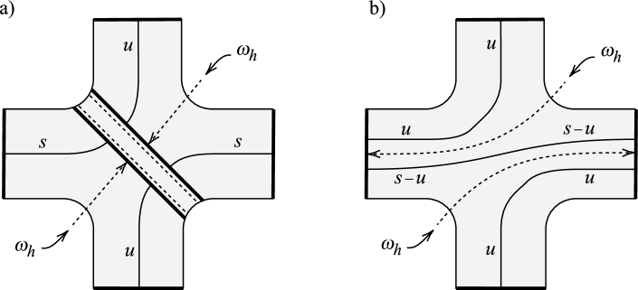
Figure 18. Two figures showing a once-punctured torus $T$ in a genus two Heegaard surface in which $T$ corresponds to a handle of an R-R diagram whose underlying Heegaard diagram has a horizontal wave $\omega_{h}$. Figure 18a illustrates a situation in which there are three nonempty bands of connections in $T$ meeting the boundary of the cutting disk $\Delta$ lying in $T$, and these bands meet $\partial\Delta$ $s$, $u$ and $s+u$ times with $s,u>0$. Figure 18b illustrates a situation in which there are only two nonempty bands of connections in $T$ and $s>u>0$. Note that, in each case, $\omega_{h}$ has an endpoint on a connection in $T$ which borders the band of connections in $T$ that meet $\partial\Delta$ maximally.

Proposition 3.2 (Horizontal Waves Terminate at Connections Bordering Band of Connections With Maximal Labels).

Suppose $\mathcal{D}_{R}$ is a genus two R-R diagram of a simple closed curve $R$ such that the Heegaard diagram $\mathbb{D}_{R}$ underlying $\mathcal{D}_{R}$ is positive, connected, and has no cut-vertex.

Suppose $T$ is a once-punctured torus handle of $\mathcal{D}_{R}$, and $\omega_{h}$ is a horizontal wave which meets $R$ in $T$. Let $\Delta$ be the cutting disk of the underlying handlebody whose boundary $\partial\Delta$ lies in $T$. Then, in each case, $\omega_{h}$ has an endpoint on a connection in $T$ which borders the band of connections with maximal label, i.e., which meet $\partial\Delta$ maximally.

Proof.

See Figures 18a and 18b, which illustrate the situation. ∎

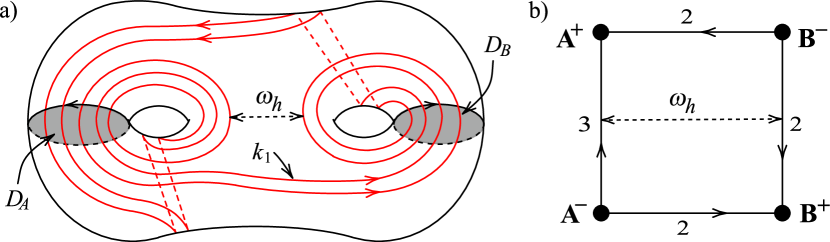
Figure 19. The horizontal wave $\omega_{h}$ based at $k_{1}$ in a genus two surface and in a Heegaard diagram

For example, consider a simple closed curve $k_{1}$ in the boundary of a genus two handlebody $H$ in Figure 19a, which is described in Section 2.2. Then its Heegaard diagram $\mathbb{D}_{k_{1}}$ shown in Figure 19b is positive, connected, and has no cut-vertex and thus it has a horizontal wave $\omega_{h}$ as in Figure 19b. In $\partial H$, $\omega_{h}$ appears as in Figure 19a. Then we can observe that as Proposition 3.2 indicates, in $\partial H$ $\omega_{h}$ terminates at the connections of $k_{1}$ with maximal intersection number $3$ in the $A$-handle and $2$ in the $B$-handle.

Figures 20, 21, 22 and 23 illustrate how an isotopy, which detours the band of connections with maximal labels on a handle, can be used to move an endpoint of a horizontal wave into the annulus between the handles of an R-R diagram.

Figure 20. Locating the attachment point of a horizontal wave $\omega_{h}$, meeting an oriented curve from the right, on a handle with three nonempty bands. Here $a,b,c,>0$, $p,q>0$ and $\gcd(p,q)=1$.

Figure 21. Locating the attachment point of a horizontal wave $\omega_{h}$, meeting an oriented curve from the right, on a handle with two nonempty bands when $p>q>0$, $a,b>0$, and $\gcd(p,q)=1$. (Note the difference between this figure and Figure 22, which shows the situation when $q>p>0$.)

Figure 22. Locating the attachment point of a horizontal wave $\omega_{h}$, meeting an oriented curve from the right, on a handle with two nonempty bands when $q>p>0$, $a,b>0$, and $\gcd(p,q)=1$. (Note the difference between this figure and Figure 21, which shows the situation when $p>q>0$.)

Figure 23. Locating the attachment point of a horizontal wave $\omega_{h}$, meeting an oriented curve from the right, on a handle with only one nonempty band. Here $a>0$, $p>r>0$ and $\gcd(p,r)=1$.

Figure 24. An R-R diagram of a nonseparating curve $R$.

In order to explain more explicitly the difference between the $p>q$ case in Figure 21 and the $p<q$ case in Figure 22, we consider a practical example. Suppose $R$ has an R-R diagram $\mathcal{D}_{R}$ of the form in Figure 24, where $a,b,c,q,r,u,t>0$, gcd$(q,r)=$gcd$(u,t)=1$, and $p=q-r,s=t-u$. One is interested in determining the range of values of the parameters $q$, $r$, $u$, and $t$ of $\mathcal{D}_{R}$ such that the manifold $H[R]$, obtained by adding a 2-handle to a genus two handlebody $H$ along $R$, embeds in $S^{3}$. The Heegaard diagram $\mathbb{D}_{R}$ underlying $\mathcal{D}_{R}$ will be positive, connected and have no cut-vertex if $q+r>2$ and $u+t>2$. If $H[R]$ embeds in $S^{3}$, then surgery on $R$ along a horizontal wave $\omega_{h}$ cuts $R$ into two disjoint simple closed curves $M_{1}$ and $M_{2}$, such that each of $M_{1}$, $M_{2}$ represents the meridian of $H[R]$. However, since $A$ appears in $R$ with only two distinct exponents, there are two subcases to consider: $q>r$ and $q<r$, and because $B$ also appears in $R$ with only two distinct exponents, there are two more subcases to consider: $u>t$ and $u<t$, for a total of four subcases to locate the horizontal wave $\omega_{h}$. Figure 25 illustrates how to locate the horizontal wave $\omega_{h}$ in these four subcases: a) $q>r$ and $u>t$, b) $q>r$ and $u<t$, c) $q<r$ and $u>t$, d) $q<r$ and $u<t$.

For example, in Figure 25a, since $q>r$ and $u>t$, $q$ and $u$ are the maximal labels in the $A$- and $B$-handles respectively. Since $\omega_{h}$ has an endpoint on a connection in one handle which borders the band of connections with maximal label, we isotope the outermost arc in the set of the $b$ parallel arcs entering the band of the $q$-connections in the $A$-handle and also isotope the outermost edge of the band of width $b$ entering the $u$-connection in the $B$-handle as shown in Figure 25a.

Figure 25. The four subcases to locate the horizontal wave $\omega_{h}$: a) $q>r$ and $u>t$, b) $q>r$ and $u<t$, c) $q<r$ and $u>t$, d) $q<r$ and $u<t$.

If $a=b=c=1$ in $\mathcal{D}_{R}$ of Figure 24, then $R=A^{r}B^{u}A^{q}B^{t}A^{q}B^{u}$ and horizontal waves leads to the following four $(M_{1},M_{2})$ pairs.

1. If $q>r$ and $u>t$, $(M_{1},M_{2})$ = $(A^{r}B^{-s}A^{r}B^{u},\,B^{t}A^{p}B^{t}A^{q})$.

2. If $q>r$ and $u<t$, $(M_{1},M_{2})$ = $(A^{r}B^{u}A^{q}B^{u}A^{r}B^{u},\,B^{s}A^{p})$.

3. If $q<r$ and $u>t$, $(M_{1},M_{2})$ = $(A^{-p}B^{-s},\,B^{t}A^{q}B^{u}A^{q}B^{t}A^{q})$.

4. If $q<r$ and $u<t$, $(M_{1},M_{2})$ = $(A^{-p}B^{u}A^{q}B^{u},\,B^{s}A^{q}B^{u}A^{q})$.

4. Culling lists of knot exterior candidates

As usual, we suppose $R$ is a nonseparating simple close curve on the boundary of a genus two handlebody $H$ with a complete set of cutting disks $\{D_{A},D_{B}\}$ such that the Heegaard diagram of $R$ with respect to $\{\partial D_{A},\partial D_{B}\}$ is connected and has no cut-vertex. If $H[R]$ embeds in $S^{3}$, then Theorem 3.1 indicates that there are two representatives $M_{1}$ and $M_{2}$ of the meridian of $H[R]$, which are obtained from $R$ by surgery along a distinguished wave based at $R$. One of the results of [B20] shows that $M_{1}$ and $M_{2}$ are “shortest” meridian representatives of $H[R]$. In other words, if a simple closed curve $m$ on $\partial H$ disjoint from $R$ represents the meridian of $H[R]$, then the complexity of the Heegaard diagram of $m$ with respect to $\{\partial D_{A},\partial D_{B}\}$ is greater than or equal to the complexity of the Heegaard diagram of either $M_{1}$ and $M_{2}$ with respect to $\{\partial D_{A},\partial D_{B}\}$.

Now we suppose that $2|M_{1}|\leq|R|$, which means that $M_{1}$ is the shortest meridian representative of $H[R]$. Then some restriction can be put as an obstruction of being the shortest meridian of $H[R]$ under some circumstances. This section is devoted to make such restriction.

We start with basic properties of nonseparating simple closed curves in a closed orientable surface.

Lemma 4.1.

Let $\alpha$ and $\beta$ be two disjoint nonseparating simple closed curves in a closed orientable surface $\Sigma$ of genus two. Then either $\alpha$ and $\beta$ are isotopic in $\Sigma$, or the union of $\alpha$ and $\beta$ does not separate $\Sigma$.

Proof.

Suppose the union of $\alpha$ and $\beta$ separates $\Sigma$. We will show this implies $\alpha$ and $\beta$ are isotopic in $\Sigma$.

Let $N_{\alpha}$ be a regular neighborhood of $\alpha$ in $\Sigma$ and let $F=\Sigma-\text{int}(N_{\alpha})$. Then $F$ is a twice-punctured torus and $\beta$ is a simple closed curve in $F$. Since we have assumed the union of $\alpha$ and $\beta$ separates $\Sigma$, $\beta$ must separate $F$. Let $N_{\beta}$ be a regular neighborhood of $\beta$ in $F$. Then $F-\text{int}(N_{\beta})$ will have two components $C_{1}$ and $C_{2}$, say. Since $\beta$ does not separate $\Sigma$, each of $C_{1}$ and $C_{2}$ must have one copy of $\alpha$ and one copy of $\beta$ as its boundary components. Then, turning to Euler characteristics, we have: $\chi(F)=-2$, while each of $\chi(C_{1})$, $\chi(C_{2})$ is even and $\leq 0$. But $\chi(F)=\chi(C_{1})+\chi(C_{2})$. Thus either $\chi(C_{1})=0$ or $\chi(C_{2})=0$. So one of $C_{1}$, $C_{2}$ is an annulus, and $\alpha$ and $\beta$ are isotopic in $\Sigma$. ∎

Lemma 4.2 (Unique Disjoint Cutting Disk).

Let $H$ be a genus two handlebody and let $\alpha$ be a simple closed curve in $\partial H$ which does not bound a disk in $H$. Let $N_{\alpha}$ be a regular neighborhood of $\alpha$ in $\partial H$. Then there is at most one nonseparating simple closed curve in $\partial H-\text{int}(N_{\alpha})$ which bounds a disk in $H$.

Proof.

First, suppose that $\alpha$ separates $\partial H$. Then each component of $\partial H-\text{int}(N_{\alpha})$ is a punctured torus and if a simple closed curve in either of these components bounds a disk in $H$, then so does $\alpha$. So, in this case, there are no nonseparating simple closed curves in $\partial H-\text{int}(N_{\alpha})$ which bound disks in $H$, and the result holds.

Next suppose $\alpha$ is nonseparating in $\partial H$, and there exist two nonseparating nonisotopic simple closed curves $\beta$ and $\gamma$, say, in $\partial H-\text{int}(N_{\alpha})$, each of which bounds a disk in $H$. We will show this implies $\alpha$ bounds a disk in $H$, contrary to hypothesis.

Note Lemma 4.1 implies that if $\beta$ and $\gamma$ are disjoint in $\partial H$, and not isotopic in $\partial H$, then $\beta$ and $\gamma$ bound a set of cutting disks for $H$. But this implies $\alpha$ also bounds a disk in $H$, contrary to hypothesis.

So $\beta$ and $\gamma$ must intersect essentially. Let $D_{\beta}$ and $D_{\gamma}$ be disks properly embedded in $H$ which are bounded by $\beta$ and $\gamma$ respectively. We may assume that $D_{\beta}$ and $D_{\gamma}$ intersect minimally and only in arcs. Let $F_{\gamma}$ be an outermost subdisk of $D_{\gamma}$ cut off of $D_{\gamma}$ by the arcs in $D_{\beta}\cap D_{\gamma}$. Since, by Lemma 4.1, $\alpha$ and $\beta$ do not separate $\partial H$, we can form a “Heegaard” diagram $\mathbb{D}_{\gamma}$ of $\gamma$ by cutting $\partial H$ open along $\alpha$ and $\beta$. By Lemma 2.1, $\mathbb{D}_{\gamma}$ must have the form shown in Figure 26. Then an examination of $\mathbb{D}_{\gamma}$ shows that $F_{\gamma}$ can be used to perform surgery on $D_{\beta}$ so as to obtain a simple closed curve $\delta$ in $\partial H$ such that $\delta$ bounds a disk in $H$ and $\delta$ is isotopic to $\alpha$. This contradicts the assumption that $\alpha$ does not bound a disk in $H$ and completes the proof. ∎

Figure 26. The Heegaard diagram $\mathbb{D}_{\gamma}$. Weights $a>0$, $c,d\geq 0$

As examples of Lemma 4.2, let $\alpha$ be a primitive curve in a genus two handlebody $H$, i.e., $H[\alpha]$ is a solid torus. Then there is a cutting disk which intersects $\alpha$ transversely at a point and thus there is another cutting disk $D$ which is disjoint from $\alpha$. By Lemma 4.2, this cutting disk $D$ is unique. On the other hand, if $\alpha$ is a Seifert curve in $H$, i.e., $H[\alpha]$ is a Seifert-fibered space and not a solid torus, then $\alpha$ must intersect every cutting disk of $H$ since $H[\alpha]$ is $\partial$-irreducible. Thus there is no cutting disk in $H$ which is disjoint from $\alpha$.

Now we describe the main result in this section which will be used in Section 5. Theorem 3.1 guarantees that a meridian $M$ of $H[R]$ can be obtained from $R$ by surgery along a distinguished wave $\omega$, provided that the Heegaard diagram $\mathbb{D}_{R}$ is connected and has no cut-vertex. Note that $H[M]$ is also a knot exterior of $S^{3}$ and thus Theorem 3.1 can apply to $M$ as well. The following lemma, which is called the Culling Lemma, provides some restriction on the shortest meridian of $H[R]$.

Lemma 4.3 (The Culling Lemma).

Let $H$ be a genus two handlebody with a complete set of cutting disks $\{D_{A},D_{B}\}$ and let $\alpha$ and $R$ be two disjoint nonseparating simple closed curves on $\partial H$. Suppose that $H[R]$ embeds in $S^{3}$ and the Heegaard diagram of $R$ with respect to $\{D_{A},D_{B}\}$ is connected and has no cut-vertex, and has a distinguished wave $\omega$ such that $\alpha$ and $\omega$ intersect essentially in a single point. Let $M_{1}$ be the representative of the meridian of $H[R]$ with $2|M_{1}|\leq|R|$, obtained from $R$ by surgery along $w$.

Suppose the Heegaard diagram of $M_{1}$ with respect to $\{D_{A},D_{B}\}$ is connected and has no cut-vertex, and has a distinguished wave $\omega_{1}$. Then $\omega_{1}$ must have more than one essential intersection with $\alpha$. Furthermore if $\omega_{1}$ has exact two essential intersections with $\alpha$, then they have same signs.

Proof.

Since $H[R]$ embeds in $S^{3}$ and $M_{1}$ is the representative of the meridian of $H[R]$, $R$ and $M_{1}$ bound a set of cutting disks of a genus two handlebody $H^{\prime}$ in $S^{3}$. Let $M_{2}$ be the other representative of the meridian of $H[R]$, obtained by surgery on $R$ along $\omega$. Since $2|M_{1}|\leq|R|$ and $|M_{1}|+|M_{2}|\leq|R|$, $|M_{1}|\leq|M_{2}|$, and, since $S^{3}$ does not contain any nonseparating $S^{2}$s, $|M_{i}|>0$ for $i=1,2$.

First we prove that $\omega_{1}$ has more than one essential intersection with $\alpha$. If $\omega_{1}$ is disjoint from $\alpha$, one of the two simple closed curves obtained from $M_{1}$ by surgery on $M_{1}$ along $\omega_{1}$ is disjoint from $\alpha$. Let $R^{\prime}$ be that curve. Then $R^{\prime}$ is a nonseparating simple closed curve in $\Sigma$, $R^{\prime}$ bounds a disk in $H^{\prime}$, and $|R^{\prime}|<|M_{1}|<|R|$. But this is impossible since by Lemma 4.2 $R$ is the unique (up to isotopy) simple closed curve in $\Sigma$ which is disjoint from $\alpha$ and bounds a disk in $H^{\prime}$. So $\omega_{1}$ must intersect $\alpha$ at least once.

Now we show that $\omega_{1}\cap\alpha$ cannot consist of just one point of essential intersection. Suppose, to the contrary, that $\omega_{1}\cap\alpha$ consists of a single point of essential intersection. Then surgery on $M_{1}$ along $\omega_{1}$ yields two nonseparating simple closed curves $M_{1,1}$ and $M_{1,2}$, each of which bounds a disk in $H^{\prime}$. One of $M_{1,1}$ and $M_{1,2}$ intersects $\alpha$ once, while the other curve intersects $\alpha$ twice. Let $M_{1,1}$ be the curve which intersects $\alpha$ once. Then $M_{1}$ and $M_{1,1}$ bound a complete set of cutting disks of $H^{\prime}$ and the Heegaard diagram of $\alpha$ with respect to $M_{1}$ and $M_{1,1}$ has the form shown in Figure 27 up to the orientations of $M_{1}$ and $M_{1,1}$.

Figure 27. The handlebody $H^{\prime}$ cut open along the set of cutting disks bounded by $M_{1}$ and $M_{1,1}$. Here $|M_{1}\cap\alpha|=1$, $\omega_{1}$ is a wave based at $M_{1}$ intersecting $\alpha$ only once, so $|M_{1,1}\cap\alpha|$ = $1$, and $R$ is the bandsum of $M_{1}$ and $M_{1,1}$ along a subarc of $\alpha$. (Note the subarc of $\omega_{1}$ with endpoints at $p$ and $q$ is a wave $\omega^{\prime}$ based at $R$.)

Since $\alpha$ intersects each of $M_{1}$ and $M_{1,1}$ only once, uniqueness of $R$ implies $R$ is the curve in Figure 27 obtained by bandsumming $M_{1}$ and $M_{1,1}$ together along a subarc of $\alpha$. Now let $\omega^{\prime}$ be the subarc of $\omega_{1}$ as shown in Figure 27 which has its endpoints at the points $p$ and $q$ of $\omega_{1}\cap R$. Then $\omega^{\prime}$ is a wave based at $R$. We claim $\omega^{\prime}$ is isotopic to $\omega$.

To see this, if the Heegaard diagram of $R$ is nonpositive with respect to $\{D_{A},D_{B}\}$, then since by Lemma 3.6 in [B20] $R$ has a unique wave, $\omega^{\prime}$ is isotopic to $\omega$. But this implies $M_{2}$ is isotopic to $M_{1,1}$, which is impossible since $|M_{1,1}|<|M_{1}|\leq|M_{2}|$. So $R$ must be positive with respect to $\{D_{A},D_{B}\}$.

Next, if the Heegaard diagram of $R$ with respect to $\{D_{A},D_{B}\}$ is positive, then $R$ has both horizontal and vertical waves, where a vertical wave is an arc one of whose endpoints lies on an edge of the Heegaard diagram $\mathbb{D}_{R}$ of $R$ connecting $A^{+}$ to one member of $\{B^{+},B^{-}\}$, while the other endpoint lies on an edge of $\mathbb{D}_{R}$ connecting $A^{-}$ to the other member of $\{B^{+},B^{-}\}$ and a horizontal wave is distinguished to be used to get a meridian of $H[R]$ by Theorem 3.1. Note that a vertical wave and a horizontal wave in the positive Heegaard diagram of $R$ intersect each other once transversely. So $\omega^{\prime}$ is either horizontal or vertical. Now $M_{1}$ is obtained from $R$ by surgery along a horizontal wave, namely $\omega$, and, as Figure 27 shows, surgery on $R$ along $\omega^{\prime}$ yields curves disjoint from $M_{1}$. This forces $\omega^{\prime}$ to be horizontal, since surgery on $R$ along a vertical wave would yield a simple closed curve having a single point of essential intersection with $M_{1}$.

Thus, again $\omega^{\prime}$ is isotopic to $\omega$. So, as before, $M_{2}$ must be isotopic to $M_{1,1}$. Since this is impossible, we conclude $\omega_{1}$ must have more than one essential intersection with $\alpha$.

Figure 28. The Heegaard diagram of $\alpha,\omega_{1}$, and $R$ with respect to $\{M_{1},M_{1,1}\}$ in Figure 28a and the Heegaard diagram of $\partial D_{A}\cup\partial D_{B}$ with respect to $\{M_{1},M_{1,1}\}$ in Figure 28b.

Now we prove the second part of the lemma, i.e, that if $\omega_{1}$ has exact two essential intersections with $\alpha$, then they have same signs. Suppose $\omega_{1}$ has exact two essential intersections with $\alpha$ with opposite intersection signs. As before, let $M_{1,1}$ and $M_{1,2}$ be two meridian representatives of $H[M_{1}]$ obtained by surgery on $M_{1}$ along $\omega_{1}$ such that $0<|M_{1,1}|<|M_{1}|$ and $0<|M_{1,2}|<|M_{1}|$. Since $M_{1}$ has one essential intersection with $\alpha$ and $\omega_{1}$ has two essential intersections with $\alpha$, one of $M_{1,1}$ and $M_{1,2}$ intersects $\alpha$ twice and the other member intersects $\alpha$ three times. Suppose $M_{1,1}$ intersects $\alpha$ three times. Then it is not hard to see that the Heegaard diagram of $\alpha$ and $\omega_{1}$ with respect to $M_{1}$ and $M_{1,1}$ has the form of Figure 28a, where $\omega_{1}$ is either $w^{+}_{1}$ or $w^{-}_{1}$. Note that since $R$ is the unique nonseparating simple closed curve disjoint from $\alpha$ which bounds a disk in $H^{\prime}$, $R$ appears as shown in Figure 28a.

Now consider the diagram obtained by adding $\partial D_{A}$ and $\partial D_{B}$ to Figure 28a. Noting that $\omega_{1}$ is disjoint from $\partial D_{A}$ and $\partial D_{B}$, while $0<|M_{1,1}|<|M_{1}|$, we see that the Heegaard diagram of $\partial D_{A}\cup\partial D_{B}$ has the form of Figure 28b. Since $0<|M_{1,1}|<|M_{1}|$, $a>0$ in Figure 28b. It follows that $|R|=c+d$ and $|M_{1}|=a+2b+c+d$. This is impossible since $|M_{1}|<|R|$. We conclude that if $\omega_{1}$ has exact two essential intersections with $\alpha$, then they have same signs. ∎

The Culling Lemma is very useful in the procedure of the classification of hyperbolic P/SF knots in $S^{3}$. From the first and the second steps for the classification, we classify all possible R-R diagrams of disjoint simple closed curve $\alpha$ and $R$ lying on the boundary of a genus two handlebody such that $\alpha$ is Seifert in $H$ and $H[R]$ is homeomorphic to the exterior of a hyperbolic knot which is represented by $\alpha$. Next step is to find a meridian representative $M$ of $H[R]$, which can be obtained from $R$ by surgery along a distinguished wave. Then the Culling Lemma applies to cull out candidates of $M$. We give an explicit example of the application of the Culling Lemma in the classification of hyperbolic P/SF knots in $S^{3}$.

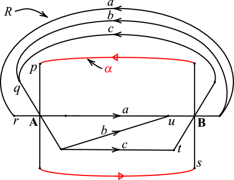
Figure 29. R-R diagram of two disjoint nonseparating simple closed curves $\alpha$ and $R$, where $q>r>0$ and $u>t>0$.

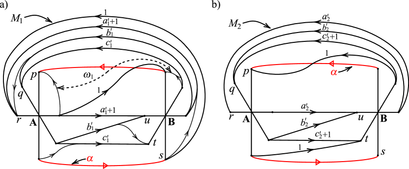
Figure 30. Two meridian representatives $M_{1}$ and $M_{2}$ of $H[R]$ obtained from $R$ by surgery along the horizontal wave $\omega_{h}$ and a horizontal wave $\omega_{1}$ based at $M_{1}$ which intersects $\alpha$ once in a).

Suppose that two disjoint simple closed curves $\alpha$ and $R$ have an R-R diagram of the form shown in Figure 29, which is the R-R diagram of $R$ in Figure 24 with the curve $\alpha$ added. Note that the curve $\alpha$ is a Seifert curve such that $H[\alpha]$ is a Seifert-fibered space over the disk with two exceptional fibers of indexes $|p|$ and $|s|$. Suppose $q>r>0$ and $u>t>0$. Then by surgery on $R$ along the horizontal wave given in Figure 25a, the two meridian representatives $M_{1}$ and $M_{2}$ have R-R diagrams as illustrated in Figure 30. Suppose $|M_{1}|\leq|M_{2}|$, i.e., $2|M_{1}|\leq|R|$.

We will show by applying for the Culling Lemma that $b^{\prime}_{1}=c^{\prime}_{1}=0$ in the R-R diagram of $M_{1}$. Suppose $b^{\prime}>0$ in Figure 30a. Then $M_{1}$ has connections with the maximal labels $q$ and $u$ in the $A$- and $B$-handles respectively and thus the Heegaard diagram of $M_{1}$ underlying the R-R diagram is connected and has no cut-vertex. Therefore there is a horizontal wave $\omega_{1}$ based at $M_{1}$ whose endpoints lie at the $q$-connection in the $A$-handle and the $u$-connection in the $B$-handle. By isotoping the both connections as in Figure 30a, the horizontal wave $\omega_{1}$ based at $M_{1}$ appears as in Figure 30a and intersects $\alpha$ transversely at a point. This is a contradiction to the Culling Lemma. So $b^{\prime}_{1}$ must be $0$ and also $c^{\prime}_{1}=0$ in the R-R diagram of $M_{1}$, otherwise $M_{1}$ can’t be a simple closed curve.

The similar argument can apply to the other representative $M_{2}$ to show that $b^{\prime}_{2}=c^{\prime}_{2}=0$ when $|M_{2}|\leq|M_{1}|$.

5. R-R diagrams of tunnel-number-one knot exteriors disjoint from proper power curves

In this section, we prove the main result of this paper, which is described in Theorem 1.1. In order to prove it, we consider a simple closed curve $R$ in the boundary of a genus two handlebody $H$ which has an R-R diagram with only one band of connections in one handle, say, $B$-handle and at most three bands of connections in the $A$-handle as shown in Figure 31 with $a,b,c\geq 0$. Note that if $s>1$ in Figure 31, there exists a proper power curve $\beta$ as shown there disjoint from $R$ with $[\beta]=B^{s}$ in $\pi_{1}(H)$. In Subsections 5.1 and  5.2, we handle R-R diagrams of $R$ of the form in Figure 31 with $a,b,c>0$ and with at least one of $a,b,c$ being $0$ but not all respectively. Throughout this section, for two disjoint nonseparating simple closed curves $c_{1}$ and $c_{2}$ in the boundary of a genus two handlebody $H$, $H[c_{1},c_{2}]$ denotes the 3-manifold obtained by adding a 2-handle to $H$ along $c_{1}$ and $c_{2}$ each and by filling in it sphere boundary with a 3-ball.

5.1. R-R diagrams of $R$ with one connection in one handle and three connections in the other handle

We consider an R-R diagram of $R$ which has only one band of connections in one handle and has three bands of connections in the other handle, i.e, an R-R diagram of $R$ of the form shown in Figure 31 with $a,b,c>0$. Then the necessary condition for $H[R]$ to embed in $S^{3}$ is given in the following Theorem.

Figure 31. An R-R diagram of $R$ where $R$ has only one band of connections in one handle and has three bands of connections in the other handle.

Theorem 5.1.

Suppose $R$ is a simple closed curve with an R-R diagram of the form shown in Figure 31 with $m,n\neq 0,(m,n)\neq(\pm 1,\pm 1)$ with the double signs in same order, $\gcd(m,n)=1$, and $|s|>1$. If $a$, $b$, and $c$ are all positive in Figure 31, then $H[R]$ cannot embed in $S^{3}$.

Proof.

Suppose, to the contrary, that there is a simple closed curve $R$ which has an R-R diagram with the form shown in Figure 31, with each of $a$, $b$, and $c$ positive, and $H[R]$ embeds in $S^{3}$. We may assume that $s>1$ because the R-R diagram of $R$ with $s<-1$ is equivalent to that with $s>1$. We divide the argument into two cases: $mn>0$ and $mn<0$.

First, suppose $mn<0$. Then the Heegaard diagram $\mathbb{D}_{R}$ of $R$ underlying the R-R diagram in Figure 31 is nonpositive. Also we see that $\mathbb{D}_{R}$ is connected and has no cut-vertex. Therefore by Theorem 3.1, one meridian representative of $H[R]$ can be obtained by surgery on $R$ along a vertical wave $\omega_{v}$. It is easy to see that one meridian representative is a simple closed curve $\beta$ as shown in Figure 31. This is a contradiction since $\beta=B^{s}$ in $\pi_{1}(H)$ with $s>1$ and $H[\beta]$ embeds in $S^{3}$ implying that $H_{1}(H[\beta])$ is torsion-free.

Now, we suppose $mn>0$. The Heegaard diagram $\mathbb{D}_{R}$ of $R$ is positive, connected, and has no cut-vertex. By using the equivalence of R-R diagrams, we may assume that $m,n>0$. Since $H[R]$ embeds in $S^{3}$, Theorem 3.1 implies that two representatives of the meridian of $H[R]$ can be obtained by surgery on $R$ along a horizontal wave $\omega_{h}$. By the results of Section 3 a horizontal wave $\omega_{h}$ based at $R$ appears in the R-R diagram as shown in Figure 32, where $0<u<s$.

Figure 32. A horizontal wave $\omega_{h}$.

Figure 33. Two representations $M_{1}$ and $M_{2}$ of the meridian of $H[R]$.

Let $M_{1}$ and $M_{2}$ be the two representatives of the meridian of $H[R]$ obtained by surgery on $R$ along $\omega_{h}$. Since $a,b,c>0$, their R-R diagrams have the form shown in Figure 33. Then examination of Figure 33 shows that $B^{s}$ appears in both $M_{1}$ and $M_{2}$. Also note that since $m,n,s,u,s-u>0$, the corresponding Heegaard diagrams of $M_{1}$ and $M_{2}$ are both positive. Now Lemmas 5.2, 5.3 and 5.11 complete the proof. ∎

Lemma 5.2.

If $|M_{1}|\leq|M_{2}|$ and $M_{1}$ does not have a cut-vertex, or if $|M_{2}|\leq|M_{1}|$ and $M_{2}$ does not have a cut-vertex, then $H[R]$ does not embed in $S^{3}$.

Proof.

Suppose $|M_{1}|\leq|M_{2}|$ and $M_{1}$ does not have a cut-vertex. Since $M_{1}$ is positive, there is a horizontal wave $\omega^{\prime}_{h}$ based at $M_{1}$. However, it is easy to see from Figure 33a that because $B^{s}$ appears in $M_{1}$, as the horizontal wave $\omega_{h}$ in Figure 32 $\omega^{\prime}_{h}$ intersects $\beta$ in a single point. This is a contradiction to the Culling Lemma of Lemma 4.3.

A similar argument works to show that if $|M_{2}|\leq|M_{1}|$, and $H[R]$ embeds in $S^{3}$, then $M_{2}$ must have a cut-vertex. ∎

Lemma 5.3.

If $M_{1}$ has a cut-vertex, then $H[R]$ does not embed in $S^{3}$.

Proof.

$M_{1}$ has the R-R diagram of the form in Figure 33a, where $A^{n}$ and $B^{s}$ appear in $M_{1}$. Because $s>1$ and $(m,n)\neq(1,1)$, $M_{1}$ can have a cut-vertex only if $A$ appears in $M_{1}$ only with exponent one and thus $b_{1}=c_{1}=0$ and $n=1$ in Figure 33a. It follows that

(5.4) $$M_{1}=B^{s-u}A(B^{s}A)^{a_{1}+1}.$$

Claim 5.5.

If $M_{1}$ has a cut-vertex, and $u>1$ in Figure 33a, then $H[R]$ does not embed in $S^{3}$.

Figure 34. The original R-R diagram of $R$ in Figure 31 with $n$ set equal to one, and with two additional simple closed curves $f$ and $\tau$ added to the diagram.

Proof of Claim 5.5.

We will show that if $M_{1}$ has a cut-vertex, and $u>1$ in Figure 33a, then $H[M_{1}]$ is Seifert-fibered over $D^{2}$ with exceptional fibers of indexes $u$ and $a_{1}+2$, and then $H[R,M_{1}]$ is Seifert-fibered over $S^{2}$ with exceptional fibers of indexes $u$, $a_{1}+2$ and $m(b+c)-c$. Since $u>1$ and $a_{1}+2>0$, it will follow that $H[R,M_{1}]$ is not $S^{3}$ once we show that $m(b+c)-c>1$.

To see that $H[M_{1}]$ is Seifert-fibered and $m(b+c)-c>1$, consider Figure 34. This figure shows the original R-R diagram of $R$ in Figure 31 with $n$ set equal to one, and with two additional simple closed curves $f$ and $\tau$ added to the diagram. Notice that if $M_{1}$ has a cut-vertex, then, since $M_{1}$ has the form shown in (5.4), i.e., the form shown in  33a with $b_{1}=c_{1}=0$ , $M_{1}$ is disjoint from both $f$ and $\tau$.

Now let $\tau(f)$ denote the simple closed curve in Figure 34 obtained from $f$ by twisting $f$ to the left $m$ times about the curve $\tau$. Then $\tau(f)$ and $M_{1}$ are disjoint, and $\tau(f)$ represents the proper power $B^{u}$ in $\pi_{1}(H)$. Note also that the automorphism of $\pi_{1}(H)$, which takes $A\mapsto B^{-s}A$ and fixes $B$, takes $M_{1}\mapsto B^{-u}A^{a_{1}+2}$. Thus by Lemma 2.2 of [D03] or Theorem 4.2 of [K20], $M_{1}$ clearly has the form of a Seifert fiber relator, i.e., $H[M_{1}]$ is Seifert-fibered with two exceptional fibers, as claimed, and the simple closed curve $\tau(f)$ represents a regular fiber of $H[M_{1}]$.

Next, another glance at Figure 34 shows that $R$ and $\tau(f)$ have $\pm(m(b+c)-c)$ algebraic intersections. But, $m>1$ and both $b$ and $c$ are positive, so clearly $m(b+c)-c>1$. This implies $H[R,M_{1}]$ is Seifert-fibered over $S^{2}$ with three exceptional fibers, and so it can’t be $S^{3}$. This concludes the proof of the claim. ∎

Claim 5.6.

If $M_{1}$ has a cut-vertex, and $u=1$ in Figure 32, then $H[R]$ does not embed in $S^{3}$.

Proof of Claim 5.6.

If $u=1$, then, as (5.4) shows, $M_{1}$ is primitive in $\pi_{1}(H)$ and $H[M_{1}]$ is a solid torus. Then $H[R,M_{1}]$ will be $S^{3}$ if and only if it is an integral homology sphere. We will show this never happens when all three weights $a$, $b$ and $c$ of the R-R diagram of $R$ in Figure 31 are positive.

The proof starts with the R-R diagram in Figure 35. This diagram shows a simple closed curve $M_{0}$ which intersects $\beta$ transversely in a single point. Note that twisting $M_{0}$ to the right $a_{1}+1$ times about the curve $\tau$ in Figure 35 transforms $M_{0}$ into the curve $M_{1}$ in Figure 33a with $b_{1}=c_{1}=0$.

Figure 35. The original R-R diagram of $R$ in Figure 31 with $u$ set equal to one, and with four additional simple closed curves $\beta$, $\tau$, $g_{1}$ and $g_{2}$ added to the diagram.

Now let $N$ be a regular neighborhood of $\beta$ and $M_{0}$ in $\partial H$, and let $N^{\prime}$ be the punctured torus $\partial H-\text{int}(N)$. Note that the curves $g_{1}$ and $g_{2}$ in Figure 35 intersect transversely at a single point and form a spine of $N^{\prime}$. Then the images $\tau(g_{1})$ of $g_{1}$ and $\tau(g_{2})$ of $g_{2}$ under Dehn twisting $a_{1}+1$ times about $\tau$ form a spine of a punctured torus in $\partial H$ which contains $R$. So if $R$ in Figure 31 has positive weights $a$, $b$ and $c$, then $[\vec{R}]=b[\tau(\vec{g}_{1})]+c[\tau(\vec{g}_{2})]$ in $H_{1}(\partial H)$.

Turning to $H_{1}(H)$, and choosing coordinates for $H_{1}(H)$ so $[\vec{A}]=(1,0)$ and $[\vec{B}]=(0,1)$ and letting $j=a_{1}+1$, we have

$$[\vec{M}_{1}] =(1,s-1)+j(1,s)$$

$$=(j+1,(j+1)s-1),\text{\quad and}$$

$$[\vec{R}] =(b(m+1),bs)+bj(1,s)+c(m,s)+cj(1,s)$$

$$=((j+m)(b+c)+b,(j+1)(b+c)s).$$

The weight $a$ of $R$ in Figure 31 is then given by $a=j(b+c)$, which will be positive if $j>0$. Then there will exist an $R$, $M_{1}$ pair with $a,b,c>0$, such that $H[R,M_{1}]$ is $S^{3}$ if and only if it is possible to choose $b,c,j>0$ and $m>1$ with $\gcd(b,c)=1$ so that

(5.7) $$(j+1)s[(j+m)(b+c)+b]=(j+1)^{2}(b+c)s+(j+m)(b+c)+b+\delta,$$

with $\delta=\pm 1$. (Note that $m>1$ since $n=1$ and $(m,n)\neq(1,1)$. The $\gcd(b,c)=1$ condition arises because $R$ is a simple closed curve; cf Lemma 5.15.)

Subtracting the $(j+1)^{2}(b+c)s$ term from both sides of (5.7) yields

(5.8) $$(j+1)s[(m-1)(b+c)+b]=(j+m)(b+c)+b+\delta.$$

We will show (5.8) can’t be satisfied by showing that the L.H.S. of (5.8) is always larger than the R.H.S. of (5.8).

Clearly (5.8) is the sum of

(5.9) $$s(j+1)(m-1)(b+c)=(j+m)(b+c),\text{\quad and}$$

(5.10) $$bs(j+1)=b+\delta.$$

Then, since $m>1$ and $s>1$, we have $js(m-1)>j$ and $(s-1)(m-1)\geq 1$. The latter inequality clearly implies $s(m-1)\geq m$. So we have $s(j+1)(m-1)>(j+m)$. Thus the L.H.S. of (5.9) is always greater than the R.H.S. of (5.9). Next, since $b>0$, $j>0$ and $s>1$, we have $b[s(j+1)-1]>1$, which implies the L.H.S. of (5.10) is always greater than the R.H.S. of (5.10). It follows that $H[R,M_{1}]$ is never $S^{3}$ when $M_{1}$ has a cut-vertex and $u=1$. So Claim 5.6 has been proved. ∎

Finally, the proofs of Claims 5.5 and 5.6 combine to prove Lemma 5.3. ∎

Lemma 5.11.

Suppose $M_{2}$ is the representative of the meridian of $H[R]$ obtained by surgery on $R$ along the horizontal wave $\omega_{h}$ shown in Figure 32. If $M_{2}$ has a cut-vertex, then $H[R]$ does not embed in $S^{3}$.

Proof.

Note that the symmetry of the original diagram of $R$ in Figure 31 shows that the arguments of Lemma 5.3, used in the case that $M_{1}$ has a cut-vertex, will also work for the case $M_{2}$ has a cut-vertex, provided minor notational changes are made. ∎

The following two lemmas deal with the exceptions for the parameters $m$ and $n$ in Theorem 5.1.

Figure 36. The R-R diagram of $R$ and its hybrid diagram.

Figure 37. The hybrid diagram of $R$ and its R-R diagram after performing a change of cutting disks inducing an automorphism of $\pi_{1}(H)$ that takes $A\mapsto AB^{-s}$.

Lemma 5.12.

Suppose $R$ and $\beta$ are simple closed curves with an R-R diagram of the form shown in Figure 31 with $(m,n)=(\pm 1,\pm 1)$ with the double signs in same order, $a,b,c>0$, and $|s|>1$. Then there is a change of cutting disks of $H$ such that $R$ and $\beta$ have an R-R diagram of the form shown in Figure 31 with $m,n\neq 0,(m,n)\neq(\pm 1,\pm 1)$, $\gcd(m,n)=1$, and $|s|>1$.

Proof.

Without loss of generality, we may assume that $(m,n)=(1,1)$ and $s>1$ in the R-R diagram of Figure 31. We use the argument of hybrid diagrams introduced in Section 2.3. The R-R diagram of $R$ and its hybrid diagram are illustrated in Figure 36. In its hybrid diagram, we drag the vertex $A^{-}$ together with the edges meeting the vertex $A^{-}$ over the $s$-connection on the $B$-handle. This performance corresponds to a change of cutting disks inducing an automorphism of $\pi_{1}(H)$ that takes $A\mapsto AB^{-s}$ and leaves $B$ fixed. The resulting hybrid diagram of $R$ is depicted in Figure 37a, where there is only one band of connections labeled by $s$ in the $B$-handle and $R$ intersects the cutting disk $D_{A}$ positively in the $A$-handle. Therefore the corresponding R-R diagram of $R$ must be the form given in Figure 37b, where $m^{\prime},n^{\prime}>0$ and $a^{\prime}+b^{\prime}+c^{\prime}=b$. We will show that $(m^{\prime},n^{\prime})\neq(1,1)$ to complete the proof.

In the R-R diagram of Figure 36a, if we read $R$ from the outermost edge of the $c$ parallel edges entering the $1$-connection in the $A$-handle, , then we can see that $R$ has subword $(AB^{s})^{i}A^{2}B^{s}$ with $i>1$. Under the automorphism $A\mapsto AB^{-s}$, the subword $(AB^{s})^{i}A^{2}B^{s}$ is sent to $A^{i+1}B^{-s}A$. This implies that the label $i+1(>2)$ appears in the $A$-handle. Thus $R$ has a band of connections with label greater than $2$ in the $A$-handle, which implies that $(m^{\prime},n^{\prime})\neq(1,1)$. ∎

Lemma 5.13.

Suppose $R$ and $\beta$ are simple closed curves with an R-R diagram of the form shown in Figure 31 with either $m=0$ or $n=0$, $a,b,c>0$, and $|s|>1$. Then there is a change of cutting disks of $H$ such that $R$ and $\beta$ have an R-R diagram of the form shown in Figure 31 with $m,n\neq 0,(m,n)\neq(\pm 1,\pm 1)$, $\gcd(m,n)=1$.

Proof.

Suppose one of $m$ and $n$ is $0$. Then without loss of generality, we may assume that $n=0$, because both cases have R-R diagrams of the same form. Then $m=1$ and the Heegaard diagram of $R$ has a cut-vertex. Note that $m$ and $n$ are not both $0$, otherwise $R$ represents $B^{ts}$ in $\pi_{1}(H)$ with $t>1$. This is impossible since $H_{1}(H[R])$ is torsion-free.

Figure 38. The Hybrid diagram and the hybrid diagram after performing a change of cutting disks inducing an automorphism of $\pi_{1}(H)$ that takes $A\mapsto AB^{-(\rho+1)s}$.

Since the Heegaard diagram of $R$ has a cut-vertex, as did in Lemma 5.12, we use the argument of hybrid diagrams. The hybrid diagram of $R$ is illustrated in Figure 38a. Let $a=\rho(b+c)+r$, where $\rho\geq 0$ and $0\leq r<b+c$. If $r=0$, then $a=\rho(b+c)$ and thus it follows from the R-R diagram of $R$ that $R$ represents $(AB^{(\rho+1)s})^{b+c}$ in $\pi_{1}(H)$, a contradiction. Therefore $r>0$. Now in the hybrid diagram, we drag $\rho+1$ times the vertex $A^{-}$ together with edges meeting the vertex $A^{-}$ over the $s$-connection on the $B$-handle. This performance corresponds to a change of cutting disks inducing an automorphism of $\pi_{1}(H)$ that takes $A\mapsto AB^{-(\rho+1)s}$. The resulting hybrid diagram of $R$ is depicted in Figure 38b, where there is only one band of connections labeled by $s$ in the $B$-handle. Also in the $A$-handle, $R$ intersects the cutting disk $D_{A}$ positively, and since $b+c-r>0$, there must be a band of connections whose label is greater than $1$. Therefore the corresponding R-R diagram of $R$ has the form of Figure 31 with $m,n\neq 0$ and $\gcd(m,n)=1$. If $(m,n)\neq(\pm 1,\pm 1)$, then by applying Lemma 5.12, we obtain an R-R diagram of $R$ with the form of Figure 31 with $m,n\neq 0,(m,n)\neq(\pm 1,\pm 1)$, $\gcd(m,n)=1$, as desired. ∎

Remark 5.14.

According to Lemmas 5.12 and 5.13, the resulting R-R diagram of $R$ obtained by performing a change of cutting disks from an R-R diagram of $R$ with the form shown in Figure 31 with $a,b,c>0$, and $|s|>1$ such that $(m,n)=(\pm 1,\pm 1)$ with the double signs in same order or either $m=0$ or $n=0$, has the form of Figure 31 with $m,n\neq 0,(m,n)\neq(\pm 1,\pm 1)$. We remark that in the resulting R-R diagram of $R$, one or two weights of $a,b,$ and $c$ might be $0$. In that case, as defined in the next section, $R$ becomes a torus or cable knot relator, which means that $H[R]$ is the exterior of a torus knot or a cable knot.

5.2. R-R diagrams of the exteriors of torus knots and tunnel-number-one cables of torus knots in $S^{3}$

Theorem 5.1 implies that if $R$ has only one band of connections with label greater than 1 on one handle, then in order for $H[R]$ to embed in $S^{3}$, $R$ must have at most two bands of connections on the other handle. In this subsection, we discuss this case, i.e., the case where $R$ has an R-R diagram of the form shown in Figure 39 and determine which values of the parameters give diagrams of embeddings in $S^{3}$.

Lemma 5.15.

Suppose $R$ is a simple closed curve with an R-R diagram of the form shown in Figure 39. If $a$ and $b$ are positive, then $\gcd(a,b)=1$.

Proof.

Observe that the simple closed curves $M$ and $\beta$ in Figure 39, intersect transversely at a single point. Then $R$ lies in a once-punctured torus $F$ in $\Sigma$, which is disjoint from $M\cup\beta$. Since $R$ represents a nontrivial homology class in the integral homology group $H_{1}(F)$, the result follows from the well-known characterization of the homology classes in $H_{1}(F)$ which are represented by simple closed curves. ∎

Figure 39. An R-R diagram of $R$ where $R$ has only one band of connections with the label greater than 1 on one handle and has at most two bands of connections on the other handle.

We first consider a positive Heegaard diagram of $R$ with no cut-vertex which underlies the R-R diagram in Figure 39 and figure out which conditions on the parameters in the R-R diagram of $R$ are required for $H[R]$ to embed in $S^{3}$.

Lemma 5.16.

Suppose $R$ is a simple closed curve with an R-R diagram of the form shown in Figure 39 with $m,n>0$, $\gcd(m,n)=1$, and $s>1$. In addition, suppose that if $a+b=1$, then $(a,b)$ = $(1,0)$ and $n>1$.

If $H[R]$ embeds in $S^{3}$, then the curve $M$ in Figure 39 represents the meridian of $H[R]$, $0<u<s$, $\gcd(s,u)=1$, and there exists $\delta=\pm 1$ such that one of the following three sets of conditions is satisfied:

1. $a+b=1$ and, (assuming without loss that $(a,b)$ = $(1,0)$), $sm-un=\delta$.
   

2. $a,b>0$, $m=1$, and $s(a+b)-u[(a+b)n+b]=\delta$.
   

3. $a,b>0$, $n>m>1$, $u=1$, and $ms(a+b)-[(a+b)n+bm]=\delta$.
   

Conversely, if one of these three sets of conditions is satisfied, then $H[M,R]$ is $S^{3}$.

Proof.

The Heegaard diagram of $R$ underlying the R-R diagram in Figure 39 is positive, connected, and has no cut-vertex. It follows from Theorem 3.1 that if $H[R]$ embeds in $S^{3}$, then a representative of the meridian of $H[R]$ can be obtained by surgery on $R$ along a horizontal wave $\omega_{h}$. The curve $M$ in Figure 39 is obtained by such a surgery on $R$, and so, if $H[R]$ embeds in $S^{3}$, $M$ represents the meridian of $H[R]$. From Figure 39, we see that $M=A^{m}B^{u}$ in $\pi_{1}(H)$ with $0<u<s$ and $\gcd(s,u)=1$. Next, consideration of the possible values of $m$ and $u$ leads to the three cases of the lemma.

First, suppose $m,u>1$. Then by Lemma 2.2 of [D03] or Theorem 4.2 of [K20], $M$ is a Seifert fiber relator, i.e., $H[M]$ is Seifert-fibered with two exceptional fibers of indexes $m$ and $u$. In addition, Figure 39 shows $R$ is a simple closed curve in $\partial H[M]$, which intersects a regular fiber of $H[M]$ $a+b$ times. This implies $H[R,M]$ will be Seifert-fibered with three exceptional fibers, and not homeomorphic to $S^{3}$, unless $a+b=1$. When $a+b=1$, we may assume $a=1$, $b=0$ and $R=A^{n}B^{s}$. It follows that $H[M,R]$ will be $S^{3}$ if and only if $sm-un=\delta$. This gives case (1) of the lemma. (Assuming $n>1$ in this case avoids the trivial situation in which $H[R]$ is a solid torus.)

Next, suppose $m=1$. Then $M$ is primitive in $H$ and $H[R,M]$ will be $S^{3}$ if and only if $H[R,M]$ is an integral homology sphere. Clearly, this happens if and only if $s(a+b)-u[(a+b)n+b]=\delta$, which gives case (2) of the lemma.

Finally, suppose $m>1$ and $u=1$. Then, again, $M$ is primitive in $H$ and $H[M,R]$ will be $S^{3}$ if and only if $H[M,R]$ is an integral homology sphere. Examination of Figure 39 shows this happens if and only if $ms(a+b)-[(a+b)n+bm]=\delta$. This gives case (3) of the lemma except for the condition that $n>m$. However, the equation $ms(a+b)-[(a+b)n+bm]=\delta$, where $\delta=\pm 1$ implies that $(n-m)(a+b)=m(s-1)(a+b)-bm-\delta$. Since $m,s>1$, the right-hand side is positive. Therefore $n>m$ as desired. ∎

Figure 40. Suppose $R$ is a simple closed curve on the boundary of a genus two handlebody $H$ such that $R$ has an R-R diagram as in this figure, with $n,s>1$, $a,b>0$, $\gcd(a,b)=1$. Then $H[R]$ is the exterior of an $(n,s)$ torus knot (Figure 40a) or an $((a+b)n+b,s)$ torus knot (Figure 40b).

To prove the next proposition, we need the following notations and lemma.

Notation. If $U=(a,b)$ is an element of $\mathbb{Z}\oplus\mathbb{Z}$, let $U^{\perp}$ denote the element $(-b,a)$ of $\mathbb{Z}\oplus\mathbb{Z}$, and let ‘$\circ$’ denote the usual inner product or dot product of vectors.

Lemma 5.17.

Let $U=(a,b)$, $V=(c,d)$ and $W=(e,f)$ be three elements of $\mathbb{Z}\oplus\mathbb{Z}$ such that $ad-bc=\pm 1$. If $W$ is expressed as a linear combination of $U$ and $V$, say $W=xU+yV$, then $y=\pm(U^{\perp}\circ W)$.

Proof.

We take an inner product by $U^{\perp}$ on both sides of $W=xU+yV$. Then since $U^{\perp}\circ U=0$ and $U^{\perp}\circ V=\pm 1$, the result follows. ∎

Proposition 5.18.

Suppose the hypothesis of Lemma 5.16. Then the curve $\beta$ in Figure 39 intersects the meridian of $H[R]$ once and two parallel copies of the curve $\beta$ bound a separating essential annulus $\mathcal{A}$ in $H[R]$, and:

1. If Case (1) of Lemma 5.16 holds, then $H[R]$ is the exterior of an $(n,s)$ torus knot in $S^{3}$, and $\beta$ represents a regular fiber in the Seifert fibration of $H[R]$.

2. If Case (2) of Lemma 5.16 holds, then $H[R]$ is the exterior of an
   $((a+b)n+bm,s)$ torus knot in $S^{3}$, and $\beta$ represents a regular fiber in the Seifert fibration of $H[R]$.

3. If Case (3) of Lemma 5.16 holds, then $H[R]$ is the exterior of an
   $(ms(a+b)\pm 1,s)$ cable about an $(a+b,m)$ torus knot in $S^{3}$ and $\mathcal{A}$ is the cabling annulus in $H[R]$.

Proof.

It is obvious from Figure 39 that the curve $\beta$ intersects the meridian of $H[R]$ once.

The diagrams of $R$ in Cases $(1)$ and $(2)$ are shown in Figures 40a and 40b respectively. Two parallel copies of the curve $\beta$ bound a separating essential annulus $\mathcal{A}$ in $H$ and thus in $H[R]$. By Lemma 2.2 of [D03] or Theorem 4.2 of [K20], $H[R]$ is a Seifert-fibered spaces over $D^{2}$ with two exceptional fibers of indexes $n$ and $s$ in Figure 40a, and $(a+b)n+b$ and $s$ in Figure 40b, and $\beta$ represents a regular fiber in the Seifert fibration of $H[R]$. However, $H[R]$ is the exterior of some knot in $S^{3}$. It is known that torus knot exteriors are Seifert-fibered, and by [MOS71], are the only knot exteriors in $S^{3}$ which are Seifert-fibered. Therefore, $H[R]$ is the exterior of a torus knot, i.e., an $(n,s)$ torus knot (Figure 40a) or an $((a+b)n+b,s)$ torus knot (Figure 40b).

Figure 41. Suppose $R$ is simple closed curve on the boundary of a genus two handlebody $H$ such that $R$ has an R-R diagram as in this figure, with $m,n,s>1$, $a,b>0$, $\gcd(a,b)$ = $\gcd(m,n)=1$, and $n(a+b)+bm$ = $sm(a+b)+\delta$ with $\delta=\pm 1$. Then $H[R]$ is the exterior of an $(ms(a+b)\pm 1,s)$ cable about an $(a+b,m)$ torus knot.

Assume that Case $(3)$ holds. The diagram of $R$ in this case is given in Figure 41. As in Cases $(1)$ and $(2)$, two parallel copies of the curve $\beta$ bound a separating essential annulus $\mathcal{A}$ in $H$ and thus in $H[R]$.

Let $\mathcal{D}$ denote the R-R diagram of Figure 41. Suppose that $D_{A}$ and $D_{B}$ are cutting disks of $H$ underlying the A-handle and B-handle respectively of $\mathcal{D}$.

Cutting $H$ open along $\mathcal{A}$ yields a solid torus $V$ and a genus two handlebody $W$. Observe that $R$ lies in $\partial W$, and $W$ has cutting disks $D_{A}$ and $D_{C}$, where $D_{C}$ is one of the outermost subdisks that $\mathcal{A}$ cuts out of $D_{B}$.

Claim 5.19.

$W[R]$ is the exterior of an $(m,a+b)$ torus knot.

Proof.

Consider the Heegaard diagram of $R$ with respect to $\{D_{A},D_{C}\}$ of $W$. Since $R$ intersects $D_{C}$ once before and after intersecting $D_{A}$, $R$ has an R-R diagram as shown in Figure 42a which the Heegaard diagram underlies. Note that the diagram of $R$ in Figure 42a can be obtained from the diagram of $R$ in Figure 41 with $s$ set equal to $1$.

Let $A$ and $C$ denote generators of $\pi_{1}(W)$ dual to the cutting disks $D_{A}$ and $D_{C}$ respectively of $W$. For the weights $a$ and $b$ in the R-R diagram of $R$, since gcd$(a,b)=1$, we can let $a=\rho b+r$, where $\rho\geq 0$ and $0\leq r<b$ (if $r=0$, then $\rho>0$ and $b=1$).

Now we record $R$ by starting the $b$ parallel arcs entering into the $(m+n)$-connection in the $A$-handle. It follows from the R-R diagram that $R$ is the product of two subwords $A^{m+n}(CA^{n})^{\rho}C$ and $A^{m+n}(CA^{n})^{\rho+1}C$ with $|A^{m+n}(CA^{n})^{\rho}C|=b-r$ and $|A^{m+n}(CA^{n})^{\rho+1}C|=r$. There is a change of cutting disks of the handlebody $W$ underlying the diagram, which induces an automorphism of $\pi_{1}(H)$ that takes $C\mapsto CA^{-n}$ and leaves $A$ fixed. Then by this change of cutting disks, $A^{m+n}(CA^{n})^{\rho}C$ and $A^{m+n}(CA^{n})^{\rho+1}C$ are sent to $A^{m}C^{\rho+1}$ and $A^{m}C^{\rho+2}$. Therefore the resulting Heegaard diagram of $R$ realizes a new R-R diagram of the form in Figure 42b, where the positions of the $A$- and $C$-handles are switched. The R-R diagram of $R$ in Figure 42b has the same form as in Figure 40b implying that $W[R]$ is the exterior of an $(a+b,m)$ torus knot in $S^{3}$. This completes the proof of the claim. ∎

Figure 42. An R-R diagram of $R$ with $s=1$ and new R-R diagram of $R$ after the change of cutting disks.

By the claim, $W[R]$ is the exterior of an $(a+b,m)$ torus knot in $S^{3}$, therefore $H[R]$ is a cable about an $(a+b,m)$ torus knot in $S^{3}$ with $\mathcal{A}$ the cabling annulus in $H[R]$.

It remains to compute the cabling coordinates. Let $l$ be the longitude of $W[R]$. Then, since $\beta$ is a boundary component of the cabling annulus $\mathcal{A}$, the cabling coordinates are given, up to sign, by $\Delta(\beta,l)$ and $\Delta(\beta,\partial D_{B})$. It is obvious that $\Delta(\beta,\partial D_{B})=s$.

Claim 5.20.

$\Delta(\beta,l)=(a+b)n+bm$.

Proof.

Let $M$ be a meridian of $W[R]$. Then $H_{1}(W[R])(=\mathbb{Z})$ is generated by $[M]$ and $[\beta]=\Delta(\beta,l)[M]$ in $H_{1}(W[R])$. Since $W[R,M]\cong S^{3}$, $\{[R],[M]\}$ is a basis of $H_{1}(W)=\mathbb{Z}\oplus\mathbb{Z}$. If we let $[\beta]=x[R]+y[M]$ in $H_{1}(W)$, then since $W[R]$ is obtained from $W$ by gluing a 2-handle along $R$, $y=\Delta(\beta,l)$. In order to compute $y$, we apply for Lemma 5.17. It follows from Figure 42a that $[\vec{R}]=((a+b)n+bm,a+b)$ and $[\vec{\beta}]=(0,1)$ in $H_{1}(W)$. Then Lemma 5.17 implies

$$y=|[\vec{R}]^{\perp}\circ[\vec{\beta}]|=|((a+b)n+bm,a+b)^{\perp}\circ(0,1)|=(a+b)n+bm.$$

This completes the claim. ∎

Therefore, $H[R]$ is an $((a+b)n+bm,s)$ cable about an $(a+b,m)$ torus knot. Since $ms(a+b)-[(a+b)n+bm]=\pm 1$, $H[R]$ is an $(ms(a+b)\pm 1,s)$ cable about an $(a+b,m)$ torus knot, as desired. ∎

We note that in Cases (1), (2), and (3), the curve $R$ is the boundary of the co-core of a 1-handle regular neighborhood of some unknotting tunnel of a torus knot for (1) and (2) and of a cable of a torus knot for (3). However since there are the classifications of unknotting tunnels of torus knots and cables of torus knots up to homeomorphism in [BRZ88] and [MS91] respectively, the converse of Proposition 5.18 is also true as the following propositions verify.

Proposition 5.21.

Suppose $R$ is a simple closed curve on the boundary of a genus two handlebody $H$ such that $H[R]$ is homeomorphic to the exterior of a torus knot in $S^{3}$. Then $R$ has an R-R diagram with the form in Figures 40a or 40b with the parameters satisfying the conditions of Cases $(1)$ and $(2)$ respectively in Lemma 5.16.

Proof.

This follows from Theorem 3.2 of [K20], which provides a classification of R-R diagrams of $R$ such that $H[R]$ is a Seifert-fibered space over the disk with two exceptional fibers.

The idea of its proof is that since $H[R]$ is homeomorphic to the exterior of a torus knot in $S^{3}$, $H[R]$ is a Seifert-fibered space $\mathcal{M}$ over the disk with two exceptional fibers and by the definition of a 2-handle addition, $H[R]$ induces a genus two Heegaard decomposition of $\mathcal{M}$. The result of [BRZ88] shows that there are three genus two Heegaard decompositions of $\mathcal{M}$ up to homeomorphism. One of them gives an R-R diagram of Figure 40a, and the other two are symmetric each other so that they boil down to an R-R diagram of Figure 40b. ∎

Proposition 5.22.

Suppose $R$ is a simple closed curve on the boundary of a genus two handlebody $H$ such that $H[R]$ is homeomorphic to the exterior of a cable of a torus knot in $S^{3}$. Then $R$ has an R-R diagram with the form in Figure 41 with the parameters satisfying the conditions of Case $(3)$ in Lemma 5.16.

Proof.

Suppose $k$ is a cable of a torus knot in $S^{3}$ whose exterior is homeomorphic to $H[R]$. Note that $k$ is a tunnel-number-one knot such that $R$ is the boundary of a cocore of the 1-handle regular neighborhood of a tunnel. In other words, the curve $R$ corresponds to a tunnel of $k$. By the result of [MS91] $k$ is an $(spq+\delta,s)$ cable of a $(p,q)$ torus knot with $\delta=\pm 1$ and has two unknotting tunnels up to homeomorphism. Here, we may assume that $p,q>1$ and $s>1$.

Claim 5.23.

There exist two simple closed curves $R_{1}$ and $R_{2}$ on $\partial H$ such that

1. $H[R_{1}]$ and $H[R_{2}]$ are homeomorphic to the exterior of the $(spq+\delta,s)$ cable of a $(p,q)$ torus knot $k$,

2. $R_{1}$ and $R_{2}$ have R-R diagrams of the form shown in Figure 41, and

3. there is no homeomorphism from $H$ onto itself sending $R_{1}$ to $R_{2}$.

Proof.

For the values $p,q,s$, and $\delta$, there are two sets of integers $(m_{1},n_{1},a_{1},b_{1})$ and $(m_{2},n_{2},a_{2},b_{2})$ with $m_{i},n_{i}>1$ and $a_{i},b_{i}>0$ for $i=1,2$ such that

$$\begin{split}&p=a_{1}+b_{1},q=m_{1},n_{1}(a_{1}+b_{1})+b_{1}m_{1}=sm_{1}(a_{1}+b_{1})+\delta,\hskip 5.69046pt\text{and}\\ &p=m_{2},q=a_{2}+b_{2},n_{2}(a_{2}+b_{2})+b_{2}m_{2}=sm_{2}(a_{2}+b_{2})+\delta.\end{split}$$

For the set of integers $(m_{i},n_{i},a_{i},b_{i})$ for $i=1,2$, we consider a simple closed curve $R_{i}$ which has an R-R diagram of the form in Figure 41 with $(m,n,a,b)=(m_{i},n_{i},a_{i},b_{i})$. Then by Proposition 5.18, $H[R_{i}]$ is homeomorphic to the exterior of $k$.

To complete the proof of the claim, it remains to show that there is no homeomorphism from $H$ onto itself sending $R_{1}$ to $R_{2}$. We can observe from an R-R diagram of the form in Figure 41 with $(m,n,a,b)=(m_{i},n_{i},a_{i},b_{i})$ that $R_{1}$ and $R_{2}$ have the Heegaard diagrams of the form shown in Figures 43a and  43b respectively. Since $p,q>1$ and $s>1$, it follows that $(s-1)pq+\delta>p$ and $(s-1)p\geq p$ for $R_{1}$, and $(s-1)pq+\delta>q$ and $(s-1)q\geq q$ for $R_{2}$. This implies that $R_{1}$ and $R_{2}$ have minimal lengths which are distinct. Therefore by the result of [W36], there is no homeomorphism from $H$ onto itself sending $R_{1}$ to $R_{2}$.

Figure 43. The Heegaard diagrams of $R_{1}$ and $R_{2}$ underlying the R-R diagrams in Figure 41.

∎

Since $k$ has two unknotting tunnels up to homeomorphism, Claim 5.23 implies that $R_{1}$ and $R_{2}$ represent the two tunnels of $k$. Therefore if $R$ is a simple closed curve on $\partial H$ such that $H[R]$ is homeomorphic to the exterior of $k$, then there exists a homeomorphism from $H$ onto itself sending $R$ to either $R_{1}$ or $R_{2}$, whose corresponding R-R diagrams are of the form in Figure 41. Therefore, $R$ has an R-R diagram with the form in Figure 41. ∎

Now we give some terminology for R-R diagrams of $R$ with the form in Figures 40 and 41.

Definition 5.24 (Torus or cable knot relators).

If a simple closed curve $R$ in the boundary of a genus two handlebody $H$ has an R-R diagram of the form shown in Figure 40 and thus $H[R]$ is the exterior of a torus knot, then $R$ is said to be a torus knot relator. In particular, if $R$ has the diagram in Figure 40a (Figure 40b, resp.), then $R$ is called a rectangular(non-rectangular, resp.) torus knot relator.

If a simple closed curve $R$ has an diagram of the form shown in Figure 41 and thus $H[R]$ is the exterior of a cable of a torus knot, then $R$ is called a cable knot relator.

5.3. Main results: R-R diagrams of tunnel-number-one knot exteriors disjoint from proper power curves

Now we prove Theorem 1.1, which is a combination of Proposition 5.18 and the following theorem. Also for convenience, we put a copy of Figure 1 in Figure 44.

Theorem 5.25.

Suppose $R$ and $\beta$ are disjoint simple closed curves in the boundary of a genus two handlebody $H$ such that $H[R]$ embeds in $S^{3}$ and $\beta$ is a proper power curve. Then $R$ and $\beta$ have an R-R diagram with the form shown either in Figure 44a with $s>1$ or Figure 44b with the set of parameters $(a,b,m,n,s)$ satisfying the hypothesis of Lemma 5.16 so that $(a,b,m,n,s)$ has the condition (1), (2), or (3) in Lemma 5.16.

Figure 44. All possible R-R diagrams of disjoint simple closed curves $R$ and $\beta$ up to homeomorphism on $H$ such that $H[R]$ embeds in $S^{3}$ and $\beta$ is a proper power curve.

Proof.

By the definition of a proper power curve, there exist an essential separating disk $D_{C}$ disjoint from $\beta$ and a complete set of cutting disks $\{D_{A},D_{B}\}$ of $H$ such that $D_{C}\cap(D_{A}\cup D_{B})=\varnothing$, $\beta\cap D_{A}=\varnothing$, and $|\beta\cap D_{B}|=s(>1)$. This implies that with respect to the set of cutting disks $\{D_{A},D_{B}\}$, $\beta$ has an R-R diagram of the form in Figure 44.

Suppose a simple closed curve $R$ is added to the R-R diagram of $\beta$. If $R$ has no connections in the $B$-handle, then $R$ has only one connection in the $A$-handle. Since $H[R]$ embeds in $S^{3}$, the label of the connection should be $\pm 1$. Therefore in this case $R$ and $\beta$ have an R-R diagram which has the form shown in Figure 44a up to equivalence.

Now suppose $R$ has connections in both $A$- and $B$-handles. Since $R$ is disjoint from $\beta$, $R$ must have an R-R diagram of the form shown in Figure 45, where $m,n\in\mathbb{Z}$ with gcd$(m,n)=1$. Then $R$ must be positive, otherwise as in the proof of Theorem 5.1, one meridian representative of $H[R]$, which is obtained by surgery on $R$ along a vertical wave, is isotopic to $\beta$, a contradiction.

Figure 45. An R-R diagram of $R$ which is disjoint from a proper power curve $\beta$ with $[\beta]=B^{s}$ in $\pi_{1}(H)$.

The positivity of $R$ implies that either $a=0$ or $d=0$. We may assume that $d=0$ and thus $R$ has an R-R diagram of the form in Figure 31 because if $a=0$, then $R$ has an R-R diagram of the same form in Figure 31.

Since $H[R]$ embeds in $S^{3}$, by Theorem 5.1 and Lemmas 5.12 and 5.13, we may assume that the R-R diagram of $R$ and $\beta$ has the form shown in Figure 44b with $ab\geq 0$ and $n,m+n\geq 0$. The condition $n,m+n\geq 0$ follows from the positivity of $R$ and the equivalence of R-R diagrams. To complete the proof, we will show that the R-R diagram of $R$ and $\beta$ in Figure 44b with $ab\geq 0$ and $n,m+n\geq 0$ is equivalent to either the R-R diagram of Figure 44a or the R-R diagram of Figure 44b with $m,n>0$, in which case the set of parameters $(a,b,m,n,s)$ satisfies the hypothesis of Lemma 5.16 as desired. Here we note that $m(>0)$ is the parameter obtained by subtracting the label of the vertical connection from the label of the horizontal connection.

First, assume that $ab=0$. We may assume that $b=0$ and thus $a=1$. If $n=0$, then $R=B^{s}$ in $\pi_{1}(H)$, a contradiction. If $n>1$, then this belongs to the case (1) in Lemma 5.16. If $n=1$, then $R=AB^{s}$ and $\beta=B^{s}$. We perform a change of cutting disk of $H$ inducing an automorphism of $\pi_{1}(H)$ which takes $A\mapsto AB^{-s}$. Then $R$ and $\beta$ are carried to $R=A$ and $\beta=B^{s}$ and it is easy to see that the resulting R-R diagram has the form of Figure 44a.

Second, assume that $ab>0$. We divide the argument into two subcases: (i) $n(m+n)>0$ and (ii) $n(m+n)=0$.

(i) Suppose $n(m+n)>0$. If $m=0$, then since $\gcd(m,n)=1$, $n=1$ and thus $R=AB^{(a+b)s}$, a contradiction. Therefore $m\neq 0$, which implies that either $m+n>n>0$ or $n>m+n>0$. If $m+n>n>0$, then $m>0$ and thus we are done. If $n>m+n>0$, then we perform an orientation-reversing homeomorphism on $H$ which switches the vertical connection labeled by $n$ and the horizontal connection labeled by $m+n$ in the $A$-handle and swaps the arc of weight $a$ and the arc of weight $b$ in the R-R diagram of $R$. Therefore the resulting R-R diagram of $R$ has the vertical connection labeled by $m+n$ and the horizontal connection labeled by $n$ with $n-(m+n)=-m>0$. Therefore the resulting R-R diagram of $R$ belongs to the form of R-R diagram of Figure 44b with $m,n>0$.

(ii) Suppose $n(m+n)=0$. Note that both $n$ and $m+n$ cannot be $0$. Therefore without loss of generality we may assume that $n+m=1$ and then $n=0$. Since $n=0$, there is a $0$-connection in the diagram of $R$. We use the argument of the hybrid diagram.

Figure 46. The Hybrid diagram corresponding to the R-R diagram in Figure 44b with $(m,n)=(1,0)$ and the hybrid diagram after performing a change of cutting disks inducing an automorphism of $\pi_{1}(H)$ that takes $A\mapsto AB^{-(\rho+1)s}$.

Its hybrid diagram of $R$ corresponding to the R-R diagram in Figure 44b with $(m,n)=(1,0)$ is illustrated in Figure 46a. Let $a=\rho b+r$, where $\rho\geq 0$ and $0\leq r<b$. Then in its hybrid diagram, we drag $\rho+1$ times the vertex $A^{-}$ together with the edges meeting with the vertex $A^{-}$ over the $s$-connection on the $B$-handle. This performance corresponds to a change of cutting disks inducing an automorphism of $\pi_{1}(H)$ that takes $A\mapsto AB^{-(\rho+1)s}$. The resulting hybrid diagram of $R$ is depicted in Figure 46b, where there is only one band of connections labelled by $s$ in the $B$-handle. Also in the $A$-handle, $R$ intersects the cutting disk $D_{A}$ positively. Note that the curve $\beta$ remains same under the change of cutting disks.

If $r=0$, then from the equation $a=\rho b+r$, $b=1$ and $a=\rho$, whence $R$ consists of only one edge connecting the vertices $A^{+}$ and $A^{-}$ in Figure 46b. This implies that $R$ and $\beta$ have the R-R diagram of Figure 44a.

Now suppose $r>0$. The corresponding R-R diagram of $R$ has the form of either Figure 31 or Figure 44b depending on the number of bands of connections that $R$ has in the $A$-handle. In either case, since $b-r>0$, there must be bands of connections whose label is greater than $1$, which indicates that there is no $0$-connection in the $A$-handle. By Theorem 5.1 and Lemma 5.12 we may assume that the R-R diagram of $R$ and $\beta$ has the form of Figure 44b. Since there is no $0$-connection in the $A$-handle, we apply exactly same argument as that in fifth and seventh paragraphs in this proof to conclude that the R-R diagram of $R$ and $\beta$ is equivalent to either the R-R diagram of Figure 44a or the R-R diagram of Figure 44b with $m,n>0$. This completes the proof. ∎

By using Theorem 1.1, we can prove the following, which is Theorem 1.2.

Theorem 5.26.

Suppose $R$ is a nonseparating simple closed curve in the boundary of a genus two handlebody such that $H[R]$ embeds in $S^{3}$. Then there exists a proper power curve disjoint from $R$ if and only if $H[R]$ is the exterior of the unknot, a torus knot, or a tunnel-number-one cable of a torus knot.

Proof.

The “if” part immediately follows from Theorem 1.1.

For the “only if” part, assume that $H[R]$ is the exterior of the unknot, a torus knot, or a tunnel-number-one cable of a torus knot. For the last two cases, by Propositions 5.22 and 5.21 $R$ has an R-R diagram of the form shown in Figure 44b with $a,b\geq 0$ and $s>1$. Hence there exists a proper power curve disjoint from $R$.

If $H[R]$ is the exterior of the unknot, then $H[R]$ is a solid torus, which implies that $R$ is primitive in $H$. Therefore, there exists a complete set of cutting disks $\{D_{A},D_{B}\}$ of $H$ such that $R$ has an R-R diagram of the form shown in Figure 44a with $s>1$. So there exists a proper power curve disjoint from $R$, completing the proof. ∎

References

- [B09] Berge, J., A classification of pairs of disjoint nonparallel primitives in the boundary of a genus two handlebody, arXiv:0910.3038. preprint.
- [B20] Berge, J., Distinguished waves and slopes in genus two, preprint.
- [B93] Berge, J., Embedding the Exteriors of One-Tunnel Knots and Links in the 3-Sphere, Unpublished transparencies of invited address at Cascade Topology Conf. Spring 1993.
- [B90] Berge, J., Some Knots with Surgeries Yielding Lens Spaces, Unpublished manuscript. Univ. of Texas at Austin, 1990.
- [B18] Berge, J., Some Knots with Surgeries Yielding Lens Spaces, arXiv preprint arXiv:1802.09722, 2018. original unpublished work from 1990.
- [B08] Berge, J., The simple closed curves in genus two Heegaard surface of which are double-primitives, Unpublished manuscript.
- [BK20] Berge, J. and Kang, S. The hyperbolic primitive/Seifert knots in , preprint.
- [BRZ88] Boileau, M., Rost, M., and Zieschang, H., On Heegaard decompositions of torus knot exteriors and related Seifert fibre spaces. Math. Ann. 279 (1988), 553–581.
- [D03] Dean, J., Small Seifert-fibered Dehn surgery on hyperbolic knots, Algebraic and Geometric Topology 3 (2003), 435–472.
- [EM92] Eudave-Muñoz, M., Band sums of links which yield composite links. The cabling conjecture for strongly invertible knots, Trans. Amer. Math. Soc. 330 no. 2, (1992), 463–501.
- [EM02] M. Eudave-Muñoz, On hyperbolic knots with Seifert fibered Dehn surgeries, Topology Appl. 121 (2002), 119–141.
- [G13] Green, J. E., The lens space realization problem, Ann. of Math. (2) 177 (2013), 449–511.
- [HOT80] Homma, T., Ochiai, M. and Takahashi, M., An Algorithm for Recognizing in 3-Manifolds with Heegaard Splittings of Genus Two, Osaka J. Math. 17 (1980), 625–648.
- [K14] Kang, S., Knots in admitting graph manifold Dehn surgeries, J. Korean Math. Soc. 51 (2014), No. 6, 1221–1250.
- [K20] Kang, S. Primitive, proper power, and Seifert curves in the boundary of a genus two handlebody, preprint.
- [MM05] Miyazaki, K. and Motegi, K., On primitive/Seifert-fibered constructions, Math. Proc. Camb. Phil. Soc. 138 (2005), 421-435.
- [MOS71] Moser, L., Elementary surgery along a torus knot, Pacific J. Math. 38 (1971) 737–745.
- [MS91] Marimoto, K., Sakuma, M., On unknotting tunnel for knots, Math. Ann. 289 (1991) 143–167.
- [O79] Ochiai, M., Heegaard-Diagrams and Whitehead-Graphs, Math. Sem. Notes of Kobe Univ. 7 (1979), 573–590.
- [OS77] Osborne, R. P. and Stevens, R. S., Group Presentations Corresponding to Spines of 3-Manifolds II, Trans. Amer. Math. Soc. 234 (1977), 213–243.
- [W36] Whitehead, J. H. C., On Equivalent Sets of Elements in a Free Group, Ann. of Math. 37 (1936), 782–800.
- [Z62] Zieschang, H., Über einfache Kurven auf Vollbrezeln, Abn. Math. Sem. Univ. Hamburg 25 (1962), 231–250.
- [Z63a] Zieschang, H., Über einfache Kurvensysteme auf Vollbrezel vom Geschlect 2, Abn. Math. Sem. Univ. Hamburg 26 (1963), 237–247.
- [Z63b] Zieschang, H., Classification of Simple Systems of Paths on a Solid Pretzel of Genus 2, Soviet Math. 4 (1963), 1460–1463. Transl. of Doklady Acad. Sci. USSR 152 (1963), 841–844.
- [Z88] Zieschang, H., On Heegaard Diagrams of 3-Manifolds, Astérisque 163-164 (1988), 247–280.