On nonhyperbolicity of P/P and P/SF knots in $S^{3}$

Abstract.

In [B90] or an available version [B18], Berge constructed twelve families of primitive/primitve(or simply P/P) knots, which are referred to as the Berge knots. It is proved in [B08] or independently in [G13] that all P/P knots are the Berge knots, which gives the complete classification of P/P knots. However, the hyperbolicity of the Berge knots was undetermined in [B90]. As a natural generalization of P/P knots, Dean introduced primitive/Seifert(or simply P/SF) knots in $S^{3}$. The classification of hyperbolic P/SF knots has been performed and the complete list of hyperbolic P/SF knots is given in [BK20].

In this paper, we provide necessary, sufficient, or equivalent conditions for P/P or P/SF knots being nonhyperbolic, and their applications on some P/SF knots. The results of this paper will be used in proving the hyperbolicity of P/P and P/SF knots in [K20a] and [K20b] completing the classification of hyperbolic P/P and P/SF knots in [B90] and [BK20] respectively.

1. Introduction

For a genus two handlebody $V$ and an essential simple closed curve $\alpha$ in $\partial V$, $V[\alpha]$ will denote the 3-manifold obtained by adding a 2-handle to $V$ along $\alpha$. An essential simple closed curve $\alpha$ in $\partial V$ is primitive in $V$ if $V[\alpha]$ is a solid torus. We say $\alpha$ is Seifert in $V$ if $V[\alpha]$ is a Seifert-fibered space and not a solid torus. Note that, since $V$ is a genus two handlebody, that $\alpha$ is Seifert in $V$ implies that $V[\alpha]$ is an orientable Seifert-fibered space over $D^{2}$ with two exceptional fibers, or an orientable Seifert-fibered space over the Möbius band with at most one exceptional fiber.

Suppose $\alpha$ is a simple closed curve lying in a genus two Heegaard surface $\Sigma$ of $S^{3}$ bounding handlebodies $H$ and $H^{\prime}$. A simple closed curve $\alpha$ in $\Sigma$ is primitive/primitive, double-primitive, or P/P, if it is primitive in both $H$ and $H^{\prime}$. Similarly, $\alpha$ is primitive/Seifert, or P/SF, if it is primitive in one of $H$ or $H^{\prime}$, say $H^{\prime}$, and Seifert in $H$. If a knot $k$ in $S^{3}$ is represented by a P/P(P/SF, resp.) simple closed curve, then we say that $k$ is a P/P(P/SF, resp.) knot and $(\alpha,\Sigma)$ is a P/P(P/SF, resp.) position of $k$. Note that a knot may have more than one P/P(P/SF, resp.) position. Also note that since $\alpha$ is primitive in one handlebody, a P/P or P/SF knot $k$ is a tunnel-number-one knot in $S^{3}$.

Let $N(k)$ be a tubular neighborhood of $k$ in $S^{3}$ and $\gamma$ a component of $\partial N(\alpha)\cap\Sigma$. Then $\gamma$ is an essential simple closed curve in $\partial N(\alpha)$. The isotopy class of $\gamma$ in $\partial N(\alpha)$ defines the surface slope in $\partial N(k)$. Note that surface slopes are integral. Then by using, for example, Lemma 2.3 in [D03], we see that for surface slopes P/P knots admit lens space Dehn surgeries and P/SF knots admit Seifert-fibered Dehn surgeries over $S^{2}$ with at most three exceptional fibers or over $\mathbb{R}\mathrm{P}^{2}$ with at most two exceptional fibers. Connected sum of lens spaces might be admitted as Dehn surgeries on P/SF knot, but by [EM92] they occur only from Dehn surgeries on nonhyperbolic P/SF knots.

P/P knots are introduced and studied by Berge [B90]. Berge constructed twelve families of P/P knots, which are referred to as the Berge knots. Then it is proved in [B08] or independently in [G13] that all P/P knots are the Berge knots. This gives the complete classification of P/P knots in $S^{3}$. However, the hyperbolicity of the Berge knots was undetermined in [B90]. Later, in [D03], Dean introduced P/SF knots in $S^{3}$, which is a natural generalization of P/P knots. The classification of hyperbolic P/SF knots has been performed for years and the complete list of hyperbolic P/SF knots has been made in [BK20].

In this paper, we provide necessary, sufficient, or equivalent conditions for P/P or P/SF knots being nonhyperbolic, and their applications on some P/SF knots. Therefore the results of this paper will be used in proving the hyperbolicity of P/P and P/SF knots in [K20a] and [K20b] completing the classification of hyperbolic P/P and P/SF knots in [B90] and [BK20] respectively.

Determining whether or not P/P or P/SF knots in $S^{3}$ are hyperbolic is based on the results of Bleiler-Litherland [BL89] or independently Wu [W90] for P/P knots, and Miyazaki and Motegi [MM05] for P/SF knots. For P/P knots in $S^{3}$ which admit lens space surgeries, Bleiler-Litherland [BL89] and independently Wu [W90] showed that if nontrivial surgery on a satellite knot $k$ in $S^{3}$ yields a lens space, then $k$ is a tunnel-number-one cable of a torus knot, and the surgery is integral. In particular, $k$ is a $(2p_{0}q_{0}\pm 1,2)$ cable of a $(p_{0},q_{0})$ torus knot.

For P/SF knots in $S^{3}$, Miyazaki and Motegi have shown in [MM05] that if a primitive/Seifert knot $k$ is not hyperbolic, then $k$ is a torus knot or a tunnel-number-one cable of a torus knot. In particular the latter is an $(sp_{0}q_{0}\pm 1,s)$-cable of a $(p_{0},q_{0})$ torus knot

Surgeries on torus knots in $S^{3}$ yielding lens space or Seifert-fibered space surgeries were completely classified by Moser in [M71]. Therefore, we have the following classification of nonhyperbolic P/P and P/SF knots.

Theorem 1.1.

If P/P or P/SF knots are not hyperbolic, then they are torus knots or $(sp_{0}q_{0}\pm 1,s)$-cable of a $(p_{0},q_{0})$ torus knot.

Theorem 1.1 enables us to determine nonhyperbolicity of P/P or P/SF knots by investigating a simple closed curve $R$ on the boundary of a genus two handlebody $H$ such that $H[R]$ is the exterior of a torus knot or a cable of torus knot. This is because if a knot $k$ has a P/P or P/SF position $(\alpha,\Sigma)$ such that $\Sigma$ bounds two handlebodies $H$ and $H^{\prime}$ and $\alpha$ is assumed to be primitive in $H^{\prime}$, then there exists a complete set of cutting disks $\{D_{M},D_{R}\}$ of $H^{\prime}$ such that the boundary $M$ of $D_{M}$ intersects $\alpha$ once and the boundary $R$ of $D_{R}$ is disjoint from $\alpha$. Note that such a cutting disk $D_{R}$ disjoint from $\alpha$ is unique in $H^{\prime}$ up to isotopy. Since $M$ intersects $\alpha$ once and $R$ is disjoint from $\alpha$, $M$ is a meridian curve of $k$ and $H[R]$ is homeomorphic to the exterior of $k$ in $S^{3}$. Therefore, the hyperbolicity of $k$ is determined by the hyperbolicity of $H[R]$.

In order to obtain necessary, sufficient, or equivalent conditions for P/P or P/SF knots being nonhyperbolic in this paper, we investigate a simple closed curve $R$ on the boundary of a genus two handlebody $H$ such that $H[R]$ is the exterior of a torus knot or a cable of torus knot by using some results of [K20c] and [K20d].

Throughout the paper, we need the background for the three diagrams: Heegaard diagrams, R-R diagrams, and hybrid diagrams. See Section 2 in [K20d] for their backgrounds.

Acknowledgement. In 2008, in a week-long series of talks to a seminar in the department of mathematics of the University of Texas as Austin, John Berge outlined a project to completely classify and describe the primitive/Seifert knots in $S^{3}$. The present paper, which provides some of the background materials necessary to carry out the project, is originated from the joint work with John Berge for the project. I should like to express my gratitude to John Berge for his support and collaboration. I would also like to thank Cameron Gordon and John Luecke for their support while I stayed in the University of Texas at Austin.

2. Torus or cable knot relators

Suppose $\alpha$ is P/P or P/SF in a genus two Heegaard splitting $(\Sigma;H,H^{\prime})$ of $S^{3}$ assuming that $\alpha$ is primitive in $H^{\prime}$ in both cases. Let $k$ be a knot in $S^{3}$ represented by $\alpha$. As explained in the introduction, since $\alpha$ is primitive in $H^{\prime}$, there is a unique cutting disk $D_{R}$ in $H^{\prime}$ such that the boundary $R$ of $D_{R}$ is disjoint from $\alpha$ and $H[R]$ is homeomorphic to the exterior of $k$ in $S^{3}$. This implies that $k$ is a tunnel-number-one knot such that $D_{R}$ is a co-core of a 1-handle regular neighborhood of some unknotting tunnel of $k$. Equivalently, the pair $(H,R)$ provides a genus two Heegaard splitting of the exterior of $k$.

Unknotting tunnels(or equivalently genus two Heegaard splittings of the exterior) of torus knots and cable of torus knots are completely understood by Boileau-Rost-Zieschang [BRZ88] or independently by Moriah [M88] for torus knots and by [MS91] for cable of torus knots. This enables us to have the following, which are results of [K20d].

Theorem 2.1.

Suppose $R$ is a simple closed curve in the boundary of a genus two handlebody $H$ such that $H[R]$ embeds in $S^{3}$. Then $H[R]$ is the exterior of a torus knot in $S^{3}$ if and only if $R$ has an R-R diagram of the form shown in Figure 1 with $n,s>1$, $a,b>0$, $\gcd(a,b)=1$.

If $R$ has an R-R diagram of the form shown in Figure 1a(1b, resp.), then $H[R]$ is the exterior of an $(n,s)$ with $n>s$$(((a+b)n+b,s),\text{resp}.)$ torus knot.

Proof.

This follows from Lemma 5.16, Proposition 5.18, and Proposition 5.21 in [K20d]. ∎

Theorem 2.2.

Suppose $R$ is a simple closed curve in the boundary of a genus two handlebody $H$ such that $H[R]$ embeds in $S^{3}$. Then $H[R]$ is the exterior of a cable knot if and only if $R$ has an R-R diagram of the form shown in Figure 2, with $m,n,s>1$, $a,b>0$, $\gcd(a,b)$ = $\gcd(m,n)=1$, and $n(a+b)+bm$ = $sm(a+b)+\pm 1$.

If $R$ has an R-R diagram of the form shown in Figure 2, then $H[R]$ is the exterior of a $(sp_{0}q_{0}\pm 1,s)$ cable of a $(p_{0},q_{0})$ torus knot in $S^{3}$, where $\{p_{0},q_{0}\}=\{m,a+b\}$.

Proof.

This follows from Lemma 5.16, Proposition 5.18, and Proposition 5.22 in [K20d]. ∎

Figure 1. Suppose $R$ is a simple closed curve in the boundary of a genus two handlebody $H$ such that $R$ has an R-R diagram as in this figure, with $n,s>1$, $a,b>0$, $\gcd(a,b)=1$. Then $H[R]$ is the exterior of an $(n,s)$ torus knot with $n>s$(Figure 1a) or an $((a+b)n+b,s)$ torus knot (Figure 1b). The converse is also true.

Figure 2. Suppose $R$ is simple closed curve in the boundary of a genus two handlebody $H$ such that $R$ has an R-R diagram as in this figure, with $m,n,s>1$, $a,b>0$, $\gcd(a,b)$ = $\gcd(m,n)=1$, and $n(a+b)+bm$ = $sm(a+b)+\delta$ with $\delta=\pm 1$. Then $H[R]$ is the exterior of aa $(sp_{0}q_{0}\pm 1,s)$ cable of a $(p_{0},q_{0})$ torus knot in $S^{3}$, with $\{p_{0},q_{0}\}=\{m,a+b\}$. The converse is also true.

If a simple closed curve $R$ on a genus two handlebody $H$ has the diagram of the form shown in Figure 1, then $R$ is said to be a torus knot relator. In particular, if $R$ has the diagram in Figure 1a (resp. Figure 1b), then $R$ is called a rectangular(resp. non-rectangular) torus knot relator. If a simple closed curve $R$ has the diagram of the form shown in Figure 2, then $R$ is called a cable knot relator.

Proposition 2.3.

Suppose $R$ is a simple closed curve in the boundary of a genus two handlebody $H$ such that $H[R]$ embeds in $S^{3}$. Let $\{D_{A},D_{B}\}$ be a complete set of cutting disks of $H$ in which the Heegaard diagram $\mathbb{D}$ of $R$ is nonpositive. If $H[R]$ is the exterior of a torus or a cable of a torus knot in $S^{3}$, then an edge $e$ can be added in $\mathbb{D}$ such that its endpoints lie at one cutting disk, and $R$ and $e$ can be oriented so that all of their intersections have the same sign.

Proof.

Theorems 2.1 and 2.2 imply that $R$ has an R-R diagram of the form in Figure 1 or 2. Let $\{D^{\prime}_{A},D^{\prime}_{B}\}$ be a complete set of cutting disks of $H$ in which the Heegaard diagram $\mathbb{D}^{\prime}$ of $R$ underlies the R-R diagram of $R$ in Figure 1 or 2. Then $\mathbb{D}^{\prime}$ is positive, i.e., all of the intersections in $R\cap\partial D^{\prime}_{A}$ and $R\cap\partial D^{\prime}_{B}$ have the same sign.

Since the Heegaard diagram $\mathbb{D}$ of $R$ with respect to $\{D_{A},D_{B}\}$ is nonpositive, $(D^{\prime}_{A}\cup D^{\prime}_{B})\cap(D_{A}\cup D_{B})$ contains essential intersections. We may assume that $D^{\prime}_{A}\cap(D_{A}\cup D_{B})$ has essential intersections. Then there must exist an outermost subdisk $D$ of $D^{\prime}_{A}$ cut off by essential intersections of $D^{\prime}_{A}\cap(D_{A}\cup D_{B})$. Since all of the intersections in $R\cap\partial D^{\prime}_{A}$ have the same sign, the arc $D\cap\partial H$ has only one type of signed intersection with $R$. This completes the proof. ∎

The parameters $m,n,$ and $s$ in the diagram of a torus or a cable knot relator $R$ in Figure 1 or 2 are restricted to positive integers. The following theorem shows that if the parameters are extended to any integers, then $H[R]$ is still nonhyperbolic.

Theorem 2.4.

Suppose $R$ is a simple closed curve in the boundary of a genus two handlebody $H$ with an R-R diagram of the form shown in Figure 3 with $a,b\geq 0$ and $m,n,s\in\mathbb{Z}$.

If $H[R]$ embeds in $S^{3}$, then $R$ is either a primitive curve, or a torus or a cable knot relator in $H$. Therefore if $k$ is a knot whose exterior is homeomorphic to $H[R]$, then $k$ is either the unknot, a torus knot or a cable of a torus knot.

Figure 3. An R-R diagram of $R$ where $R$ has only one band of connections in one handle and has at most two bands of connections in the other handle and $a,b\geq 0$ and $m,n,s\in\mathbb{Z}$.

Proof.

Consider the R-R diagram of $R$ in Figure 3. Then we may assume without loss of generality that $m,s\geq 0$.

If $m=0$, then $n=1$. This implies that $R=(AB^{s})^{a+b}$ in $\pi_{1}(H)$. Since $H[R]$ embeds in $S^{3}$, for the homological reason, $a+b=1$ and thus $R$ is primitive. If $s=0$, then $R=A^{(a+b)n+bm}$ in $\pi_{1}(H)$. For the homological reason, $|(a+b)n+bm|=1$ and $R$ is primitive. If $ab=0$, then without loss of generality, we may assume that $a=1$ and $b=0$ and thus the diagram of $R$ is a rectangular torus knot relator unless $|n|=1$ or $s=1$, in which case $R$ is primitive.

Thus we may assume that $m,s>0$ and $ab>0$. Let $a=\rho b+r$, where $\rho\geq 0$ and $0\leq r<b$ (if $r=0$, then $\rho>0$ and $b=1$). We divide the argument into two subcases: (1) $s=1$ and (2) $s>1$.

Figure 4. An R-R diagram of $R$ with $s=1$ and new R-R diagram of $R$ after the change of cutting disks.

(1) Suppose $s=1$. Then the R-R diagram of $R$ is given in Figure 4a. It follows that $R$ is the product of two subwords $BA^{n}$ and $BA^{m+n}$ with $|BA^{n}|=a$ and $|BA^{m+n}|=b$. Here, $|BA^{n}|$ and $|BA^{m+n}|$ denote the total number of appearances of $BA^{n}$ and $BA^{m+n}$ respectively in the word of $R$ in $\pi_{1}(H)=F(A,B)$. We perform a change of cutting disks of $H$ underlying the diagram, which induces an automorphism $\theta$ of $\pi_{1}(H)$ that takes $B\mapsto BA^{-n}$ and leaves $A$ fixed. Then the new R-R diagram realized by the resulting Heegaard diagram of $R$ is shown as in Figure 4b. If $m>1$ in the diagram, then $R$ belongs to a torus knot relator. If $m=1$, then when $r=0$, $R=BA^{\rho+1}$ in $\pi_{1}(H)$ and thus is primitive, and when $r>0$, by Lemma 3.5 of [K20c], $R$ is also primitive in $H$.

(2) Suppose $s>1$. If $n(m+n)>0$, then by Theorems 2.1 and 2.2 $R$ is a torus or a cable knot relator. If $n(m+n)<0$, then the underlying Heegaard diagram of $R$ is nonpositive and thus there exists a vertical wave based at $R$. By one of the results of [B20], which is originated from [B93], one meridian curve of $H[R]$ is obtained by the surgery on $R$ along the vertical wave. We can see from the R-R diagram of $R$ that such meridian curve of $H[R]$ is the curve whose first homotopy is $B^{s}$ in $\pi_{1}(H)$. This is impossible since $s>1$ and $H[M]$ embeds in $S^{3}$. Therefore $n(m+n)\geq 0$.

Figure 5. The Hybrid diagram corresponding to the R-R diagram in Figure 3 with $(m,n)=(1,0)$ and the hybrid diagram after performing a change of cutting disks inducing an automorphism of $\pi_{1}(H)$ that takes $A\mapsto AB^{-(\rho+1)s}$.

Now suppose $n(m+n)=0$. Note that both $n$ and $m+n$ cannot be $0$. Therefore without loss of generality we may assume that $n+m=1$ and then $n=0$. Since $n=0$, there is a $0$-connection in the diagram of $R$. If $r=0$ in the equation $a=\rho b+r$, then $b=1$ and $R=AB^{(\rho+1)s}$, which is primitive. So we may assume that $r>0$ in the equation $a=\rho b+r$.

Now we use the argument of the hybrid diagram. Its hybrid diagram of $R$ corresponding to the R-R diagram in Figure 3 with $(m,n)=(1,0)$ is illustrated in Figure 5a. In its hybrid diagram, we drag $\rho+1$ times the vertex $A^{-}$ together with the edges meeting with the vertex $A^{-}$ over the $s$-connection on the $B$-handle. This performance corresponds to a change of cutting disks inducing an automorphism of $\pi_{1}(H)$ that takes $A\mapsto AB^{-(\rho+1)s}$. The resulting hybrid diagram of $R$ is depicted in Figure 5b, where there is only one band of connections labelled by $s$ in the $B$-handle. For the $A$-handle in the corresponding R-R diagram of $R$, since $R$ intersects the cutting disk $D_{A}$ positively and $b-r>0$, $R$ is positive and thus there are at most three bands of connections and one of the bands of connections has a label greater than $1$. If there are three bands of connections in $A$-handle, then by Theorem 5.1 in [K20d], $H[R]$ cannot embed in $S^{3}$. If there are at most two bands of connections in $A$-handle, then $R$ is a torus or a cable knot relator. ∎

Theorem 2.4 says that if $R$ has only one connection on one handle and has at most two connections on the other handle, then $H[R]$ is not hyperbolic.

3. Presentations of a torus or a cable knot relator

Suppose $H$ is a genus two handlebody with a complete set of cutting disks $\{D_{A},D_{B}\}$ with $\pi_{1}(H)=F(A,B)$, where the generators $A$ and $B$ are dual to $D_{A}$ and $D_{B}$ respectively. Suppose $R$ is a simple closed curve on $\partial H$ such that $H[R]$ embeds in $S^{3}$. Then $R$ represents a relator in $\pi_{1}(H)=F(A,B)$, i.e., $\pi_{1}(H[R])=\langle A,B\,|\,R\rangle$. In this section, we deal with some backgrounds of two generator presentations and equivalent presentation conditions for $R$ being a torus or a cable knot relator.

3.1. Backgrounds of two generator presentations

Suppose $\mathcal{P}$ is a finite presentation of a two generator set $G$. Let $F$ be the free group freely generated by the two generators in $G$. If $\mathcal{R}$ is a relator of a presentation $\mathcal{P}$ which is freely and cyclically reduced, then the algebraic length of $\mathcal{R}$ is the total number of letters which appear in $\mathcal{R}$. The algebraic length of $\mathcal{P}$, denoted by $|\mathcal{P}|$, is the sum of the lengths of all of the relators in $\mathcal{P}$. The presentation $\mathcal{P}$ has minimal algebraic length under automorphisms of $F$ if applying any automorphism of $F$ to $\mathcal{P}$ and then freely and cyclically reducing the relators of the result, yields a presentation $\mathcal{P}^{\prime}$ with $|\mathcal{P}^{\prime}|\geq|\mathcal{P}|$.

For a free group $F(A,B)$ generated by $A$ and $B$, the automorphisms

(3.1) $$(A,B)\mapsto(AB^{\pm 1},B)$$

$$(A,B)\mapsto(A,BA^{\pm 1})$$

of $F(A,B)$ are called T-transformations or Whitehead automorphisms.

Suppose $\mathcal{P}$ is a presentation which has minimal algebraic length. If a Whitehead automorphism $\theta$ transforms $\mathcal{P}$ into a presentation $\mathcal{P}^{\prime}$ such that $|\mathcal{P}^{\prime}|=|\mathcal{P}|$, then $\theta$ is called a level-T-transformation or simply a level-transformation.

The following theorems are well-known results of Whitehead [W36].

Theorem 3.2.

Let $\mathcal{P}$ and $F$ be defined as above. Suppose that all the relators in $\mathcal{P}$ are freely and cyclically reduced. If there is an automorphism of the free group $F$ which reduces the length of $\mathcal{P}$, then there exists a Whitehead automorphism which will also reduce the length of $\mathcal{P}$.

Theorem 3.3.

Let $\mathcal{P}$, $G$, and $F$ be defined as above and $\mathcal{P}^{\prime}$ be another finite presentation of $G$ such that the relators of both $\mathcal{P}$ and $\mathcal{P}^{\prime}$ are freely and cyclically reduced. Suppose both $\mathcal{P}$ and $\mathcal{P}^{\prime}$ have minimal length, and suppose there exists an automorphism $\pi$ of $F$ such that $\pi(\mathcal{P})=\mathcal{P}^{\prime}$. Then there exists a finite sequence of level-transformations which also transforms $\mathcal{P}$ to $\mathcal{P}^{\prime}$.

Suppose $\mathcal{P}=\langle\,A,B\,|\,\mathcal{R}_{1},\dots,\mathcal{R}_{m}\,\rangle$ is a two generator finitely related presentation. The Whitehead graph $G_{W}(\mathcal{P})$ of $\mathcal{P}$ is defined as follows. First, $G_{W}(\mathcal{P})$ has four vertices, labeled $A^{+}$, $A^{-}$, $B^{+}$, and $B^{-}$. Then $G_{W}(\mathcal{P})$ has one unoriented edge joining vertex $x$ and vertex $y^{-1}$ of $G_{W}(\mathcal{P})$ corresponding to each appearance of $xy$ as a subword of a relator of $\mathcal{P}$. Note that if $\mathcal{R}$ is a relator of $\mathcal{P}$ and $\mathcal{R}$ = $x_{1}x_{2}\dots x_{n}$, with $x_{i}\in\{A,A^{-},B,B^{-}\}$, then the pair $x_{n}x_{1}$ also contributes an edge to $G_{W}(\mathcal{P})$. Note also that if $\mathcal{R}=X$, with $X$ = $A^{\pm 1}$ or $B^{\pm 1}$, then $\mathcal{R}$ contributes one edge, joining vertex $X^{+}$ and vertex $X^{-}$, to $G_{W}(\mathcal{P})$.

A loop in $G_{W}(\mathcal{P})$ is an edge of $G_{W}(\mathcal{P})$ with both of its endpoints at the same vertex of $G_{W}(\mathcal{P})$. Thus, if the relators of $\mathcal{P}$ are freely and cyclically reduced, then each edge of $G_{W}(\mathcal{P})$ has its endpoints at distinct vertices of $G_{W}(\mathcal{P})$, and there are no loops in $G_{W}(\mathcal{P})$.

A finite graph $G$ is connected if given any two distinct vertices, say $V$ and $V^{\prime}$, of $G$, there is a path consisting of a finite union of edges of $G$ connecting $V$ to $V^{\prime}$.

A vertex $V$ of a finite connected graph $G$ is a cut-vertex of $G$ if deleting $V$, and the edges of $G$ which meet $V$, from $G$ yields a graph $G^{\prime}$, which is not connected.

Figure 6. The three types of graphs of Heegaard diagrams of simple closed curves on the boundary of a genus two handlebody $H$ which have essential intersections with cutting disks $D_{A}$ and $D_{B}$.

Proposition 3.4.

Suppose $\mathcal{P}$ is a two-generator presentation, which has a Whitehead graph of the form of Figure 6a. Then

1. $\mathcal{P}$ has minimal algebraic length under automorphisms if and only if $|a-b|\leq c$ and $|a-b|\leq d$.

2. $\mathcal{P}$ has a level-transformation if and only if either $|a-b|=c$ or $|a-b|=d$.

Furthermore, if $|a-b|<c$ and $|a-b|=d(|a-b|=c$ and $|a-b|<d$, resp.$)$, then only level-transformations are the Whitehead automorphisms $(A,B)\mapsto(A,BA^{\pm 1})$ $((A,B)\mapsto(AB^{\pm 1},B)$, resp.$)$.

Proof.

Theorems 3.2 implies that we need only to see how algebraic length of $\mathcal{P}$ changes under the Whitehead automorphisms. The algebraic length of $\mathcal{P}$ in Figure 6a is $2a+2b+c+d$. It is not hard to show that if we apply the Whitehead automorphism $\theta_{1}:(A,B)\mapsto(AB,B)$ to $\mathcal{P}$, then algebraic length of $\theta_{1}(\mathcal{P})$ is $3a+b+2c+d$. Similarly, the Whitehead automorphisms $\theta_{2}:(A,B)\mapsto(AB^{-1},B)$, $\theta_{3}:(A,B)\mapsto(A,BA)$, and $\theta_{4}:(A,B)\mapsto(A,BA^{-1})$ change the algebraic length of $\mathcal{P}$ to $a+3b+2c+d$, $3a+b+c+2d$, and $a+3b+c+2d$ respectively. Therefore $2a+2b+c+d$ is minimal algebraic length of $\mathcal{P}$ if and only if

(3.5) $$2a+2b+c+d\leq 3a+b+2c+d(\Leftrightarrow b-a\leq c),$$

$$2a+2b+c+d\leq a+3b+2c+d(\Leftrightarrow a-b\leq c),$$

$$2a+2b+c+d\leq 3a+b+c+2d(\Leftrightarrow b-a\leq d),$$

$$2a+2b+c+d\leq a+3b+c+2d(\Leftrightarrow a-b\leq d).$$

Then the inequalities in (3.5) complete the proof. ∎

Let $H$ be a genus two handlebody with a complete set of cutting disks $\{D_{A},D_{B}\}$ with $\pi_{1}(H)=F(A,B)$, $\mathcal{R}=\{R_{1},\ldots,R_{n}\}$ be a set of pairwise disjoint simple closed curves on $\partial H$ which have essential intersections with $D_{A}\cup D_{B}$. Let $\mathbb{D}_{\mathcal{R}}$ be a Heegaard diagram of $\mathcal{R}$ with respect to $\{D_{A},D_{B}\}$ and $[R_{i}]$ be a presentation represented by $R_{i}$ in $\pi_{1}(H)=F(A,B)$. Then we have a two-generator presentation $\mathcal{P}_{\mathcal{R}}=\langle\,A,B\,|\,[R_{1}],\ldots,[R_{n}]\,\rangle$. The geometric length of the Heegaard diagram $\mathbb{D}_{\mathcal{R}}$, denoted by $|\mathbb{D}_{\mathcal{R}}|$ is defined to be the total number of edges in $\mathbb{D}_{\mathcal{R}}$.

The following theorems are well-known results of Zieschang [Z70].

Theorem 3.6.

Let $H,\mathcal{R}$, and $\mathcal{P}_{\mathcal{R}}$ be defined as above. If there is an automorphism of the free group $F(A,B)$ which reduces the algebraic length of $\mathcal{P}_{\mathcal{R}}$, then there exists a change of cutting disks of $H$ inducing one of the Whitehead automorphisms in (3.1) which also reduce the geometric length of $\mathbb{D}_{\mathcal{R}}$.

Note that a change of cutting disks inducing a Whitehead automorphism can be achieved by replacing one cutting disk $D$ by a cutting disk $D^{\prime}$ which is obtained by bandsumming $D$ with another cutting disk along an arc connecting them. In terms of the terminology in [W36] and [Z70], such changes of cutting disks of $H$ described in Theorem 3.6 is called geometric-T-transformation of $H$. If a geometric-T-transformation of $H$ carries a geometric minimal Heegaard diagram $\mathbb{D}$ to another Heegaard digarm $\mathbb{D}^{\prime}$ with $|\mathbb{D}^{\prime}|=|\mathbb{D}|$, then it is called a level-geometric-T-transformation, or simply level-geometric-transformation.

Theorem 3.7.

Let $H,\mathcal{R}$, $\mathbb{D}_{\mathcal{R}}$, and $\mathcal{P}_{\mathcal{R}}$ be defined as above. Suppose $\mathcal{P}_{\mathcal{R}}$ has minimal algebraic length, $|\mathbb{D}_{\mathcal{R}}|=|\mathcal{P}_{\mathcal{R}}|$, and $\mathcal{P^{\prime}}_{\mathcal{R}}$ is a presentation obtained from $\mathcal{P}_{\mathcal{R}}$ by a level-transformation. Then there exists a level-geometric-transformation which carries $\mathbb{D}_{\mathcal{R}}$ into $\mathbb{D^{\prime}}_{\mathcal{R}}$ such that $|\mathbb{D^{\prime}}_{\mathcal{R}}|=|\mathcal{P^{\prime}}_{\mathcal{R}}|$, and $\mathbb{D^{\prime}}_{\mathcal{R}}$ realizes $\mathcal{P^{\prime}}_{\mathcal{R}}$.

Corollary 3.8.

Let $H,\mathcal{R}$, $\mathbb{D}_{\mathcal{R}}$, and $\mathcal{P}_{\mathcal{R}}$ be defined as above. Suppose that $\mathcal{P}_{\mathcal{R}}$ has minimal algebraic length. If $\mathcal{P}_{\mathcal{R}}$ has no level-transformations, then the complete set of cutting disks $\{D_{A},D_{B}\}$ is unique such that $\mathcal{P}_{\mathcal{R}}$ is minimal.

Proof.

This follows from Theorem 3.7. ∎

Regarding Proposition 3.4, we note that if $\mathbb{D}_{\mathcal{R}}$ has a graph of the form of Figures 6a or 6b, then $\mathbb{D}_{\mathcal{R}}$ realizes $\mathcal{P}_{\mathcal{R}}$. Therefore the graph $\mathbb{D}_{\mathcal{R}}$ of the form of Figure 6a or and 6b is the Whitehead graph of $\mathcal{P}_{\mathcal{R}}$.

3.2. Presentations of a torus or a cable knot relator

Suppose $R$ is a simple closed curve in the boundary of a genus two handlebody $H$ such that $H[R]$ embeds in $S^{3}$. We have shown that if $H[R]$ is the exterior of a torus or a cable knot in $S^{3}$, then $R$ has an R-R diagram with the form of Figure 1 or 2. The following theorem provides a strategy to determine whether or not $H[R]$ is the exterior of a torus or a cable knot.

Figure 7. The Whitehead graphs of $R$ corresponding to Figures 1 and 2.

Theorem 3.9.

Suppose $R$ is a simple closed curve in the boundary of a genus two handlebody $H$ such that $H[R]$ is the exterior of a torus or a cable knot in $S^{3}$, and a complete set of cutting disks $\{D_{A},D_{B}\}$ of $H$ intersects $R$ minimally. Let $\mathcal{P}_{R}$ be the two-generator presentation $\pi_{1}(H[R])=\langle\,A,B\,|\,[R]\,\rangle$

If $R$ has no level-transformations in $\mathcal{P}_{R}$, then the R-R diagram of $R$ with respect to $\{D_{A},D_{B}\}$ has the form of Figure 1 or 2 up to the homeomorphisms of $H$ inducing the automorphisms exchanging $A$ and $B$, and replacing $A^{-1}$ by $A$ or $B^{-1}$ by $B$.

If $R$ has a level-transformation in $\mathcal{P}_{R}$, then there is an automorphism on $\pi_{1}(H)=F(A,B)$ of form $A\mapsto AB^{p}$ or $B\mapsto BA^{q}$ which carries $R$ to a curve with an R-R diagram of the form of Figure 1 or 2 with $s=2$ up to the homeomorphisms of $H$ inducing the automorphisms exchanging $A$ and $B$, and replacing $A^{-1}$ by $A$ or $B^{-1}$ by $B$.

Proof.

The Whitehead graphs of $R$ corresponding to Figures 1 and 2 appear as Figure 7 respectively, where $c=(n-1)(a+b)+b,d=(s-1)(a+b)$ in Figure 7b and $e=(n-1)(a+b)+mb,f=(s-1)(a+b)$ in Figure 7c. The conditions on $n,m,s$ given by Theorems 2.1 and 2.2, and Proposition 3.4 imply that $R$ has minimal length under automorphisms and has no level-transformations unless $s=2$. It follows from Corollary 3.8 that the set of cutting disks $\{D_{A},D_{B}\}$ of $H$ yielding the R-R diagrams of Figures 1 and 2 is unique such that $R$ has minimal. Therefore $R$ in the hypothesis must have the R-R diagram of Figure 1 or 2.

Now we assume that $s=2$ in each R-R diagram of Figures 1 and 2. Then $R$ has minimal length under automorphisms and has level-transformations.

First consider Figure 7a with $s=2$. Then $R=A^{n}B^{2}$. It is easy to see by applying the Whitehead automorphisms that the Whitehead automorphism $\theta:B\mapsto BA^{-1}$ is only level-transformation. Therefore the automorphisms keeping the algebraic length of $R$ unchanged are of the form $\theta^{p}=B\mapsto BA^{-p}$ with $1\leq p\leq n$. If $p=n$, then the automorphism $B\mapsto BA^{-p}$ carries $R=A^{n}B^{2}$ to $A^{-n}B^{2}$, which is the same form. Therefore we may assume $1\leq p<n$. Now we need to show that the only automorphisms of the image of $R$ under $B\mapsto BA^{-p}$ which leaves the algebraic length of $R$ unchanged are of the form $B\mapsto BA^{q}$. However this is true by Proposition 3.4 because the image of $R$ under $B\mapsto BA^{-p}$ is $A^{n-p}BA^{-p}B$, whose Whitehead graph has the form shown in Figure 8a.

Figure 8. The Whitehead graphs of of the image of $R$ under the automorphism $B\mapsto BA^{-p}$.

Second consider Figure 7b with $s=2$, where $c=(n-1)(a+b)+b,d=(s-1)(a+b)$. Then $|B^{2}A^{n}|=a$ and $|B^{2}A^{n+1}|=b$ and it follows by applying the Whitehead automorphisms that the only level-transformations fixing the algebraic length of $R$ are of the form $B\mapsto BA^{-p}$ with $1\leq p\leq n$. On the other hand, $BA^{-p}BA^{n-p}$ with $|BA^{-p}BA^{n-p}|=a$ and $BA^{-p}BA^{n+1-p}$ with $|BA^{-p}BA^{n+1-p}|=b$ appear in the image of $R$ under the automorphism $B\mapsto BA^{-p}$. Its Whitehead graph appears as in Figure 8b with $c=(n-2)(a+b)+b$ or Figure 8c with $c=(n-1)(a+b)$ depending on the value of $p$, i.e., $p<n$ or $p=n$. In either of the Whitehead graphs, Proposition 3.4 implies that the only automorphisms of the image of $R$ under $B\mapsto BA^{-p}$ which leaves the algebraic length of $R$ unchanged are of the form $B\mapsto BA^{q}$.

Lastly, we consider Figure 7c with $s=2$, where $e=(n-1)(a+b)+mb,f=(s-1)(a+b)$. However if $m=1$, then this becomes the second case. Therefore we can apply the similar argument to show that the only level-transformations fixing the algebraic length of $R$ are of the form $B\mapsto BA^{-p}$ with $1\leq p\leq n$, and the only automorphisms of the image of $R$ under $B\mapsto BA^{-p}$ which leaves the algebraic length of $R$ unchanged are of the form $B\mapsto BA^{q}$. ∎

4. Proper power curves and Nonhyperbolicity

A simple closed curve $\beta$ in the boundary of a genus two handlebody $H$ is said to be a proper power curve if $\beta$ is disjoint from a separating disk in $H$, does not bound a disk in $H$, and is not primitive in $H$. Equivalently, $\beta$ represents a proper power of a primitive element in $\pi_{1}(H)$. Proper power curves play a very essential role in the classification of hyperbolic P/P and P/SF knots. In particular, the following theorem says that nonhyperbolicity of P/P and P/SF knots is equivalent to the existence of proper power curves.

Theorem 4.1.

Suppose $R$ is a simple closed curve in the boundary of a genus two handlebody $H$ such that $H[R]$ embeds in $S^{3}$. Then $H[R]$ is the exterior of the unknot, a torus knot, or a cable knot if and only if there exists a proper power curve $\beta$ in $H$ disjoint from $R$.

Proof.

This is Theorem 5.26 in [K20d]. ∎

Proposition 4.2.

Let $\alpha$ be a P/P or P/SF simple closed curve in a genus two Heegaard splitting $(\Sigma;H,H^{\prime})$ of $S^{3}$ assuming that $\alpha$ is primitive in $H^{\prime}$ in both cases, and $k$ be a knot in $S^{3}$ represented by $\alpha$. Let $R$ be a unique simple closed curve in $\partial H$ such that $R$ is disjoint from $\alpha$ and bounds a cutting disk of $H^{\prime}$.

Then $k$ is not hyperbolic if and only if there exists a proper power curve $\beta$ in $H$ disjoint from $R$.

Proof.

Assume that $k$ is not hyperbolic. By Theorem 1.1, $k$ is a torus or cable of a torus knot. Note that in Theorem 1.1, the unknot is considered as a torus knot. Since $H[R]$ is the exterior of $k$ in $S^{3}$, $H[R]$ is the unknot, a torus knot, or a cable of a torus knot. Therefore $k$ is not hyperbolic if and only if $H[R]$ is the unknot, a torus knot, or a cable of a torus knot. Then Theorem 4.1 completes the proof. ∎

Since the existence of a proper power curve indicates the nonhyperbolicity of P/P and P/SF knots, for a given R-R diagram of a curve $R$ in the boundary of a genus two handlebody, it is useful to determine whether or not there is a proper power curve $\beta$ disjoint from $R$.

Based on the following minor generalization of a result of Cohen, Metzler, and Zimmerman, we are able to classify all possible R-R diagrams of a proper power curve $\beta$ for any complete set of cutting disks of a genus two handlebody $H$.

Theorem 4.3.

[CMZ81] Suppose a cyclic conjugate of

$$W=A^{n_{1}}B^{m_{1}}\dots A^{n_{l}}B^{m_{l}}$$

is a member of a basis of $F(A,B)$ or a proper power of a member of a basis of $F(A,B)$, where $l\geq 1$ and each indicated exponent is nonzero. Then, after perhaps replacing $A$ by $A^{-1}$ or $B$ by $B^{-1}$, there exists $e>0$ such that:

$$n_{1}=\dots=n_{l}=1,\quad\text{and}\quad\{m_{1},\dots,m_{l}\}\subseteq\{e,e+1\},$$

or

$$\{n_{1},\dots,n_{l}\}\subseteq\{e,e+1\},\quad\text{and}\quad m_{1}=\dots=m_{l}=1.$$

Theorem 4.4.

Suppose $H$ is a genus two handlebody with a complete set of cutting disks $\{D_{A},D_{B}\}$ with $\pi_{1}(H)=F(A,B)$, where the generators $A$ and $B$ are dual to $D_{A}$ and $D_{B}$ respectively. If $\beta$ is a proper power curve in $H$ which has only essential intersections with $D_{A}$ and $D_{B}$, then $\beta$ has one of the following R-R diagrams with respect to the complete set of cutting disks $\{D_{A},D_{B}\}$ up to the homeomorphisms of $H$ inducing the automorphisms exchanging $A$ and $B$, and replacing $A^{-1}$ by $A$ or $B^{-1}$ by $B$:

1. Type I: $\beta$ has an R-R diagram with a $0$-connection in at least one of the handles.

2. Type II: $\beta$ has an R-R diagram of the form shown in Figure 9 with $s>1$.

3. Type III: $\beta$ has an R-R diagram of the form shown in Figure 10 with $a,b>0$ and $s>0$.

4. Type IV: $\beta$ has an R-R diagram of the form shown in Figure 11 with $a,b,c>0$.

5. Type V: $\beta$ has an R-R diagram of the form shown in Figure 12 with $a,b,c,d>0$.

Proof.

This is Theorem 1.3 of [K20c]. ∎

Figure 9. Type II of proper power curves $\beta$, where $s>1$.

Figure 10. Type III of proper power curves $\beta$: $[\beta]=(AB^{s})^{a+b}$, where $s>0$ and $a,b>0$.

Figure 11. Type IV of proper power curves $\beta$: $[\beta]=(AB)^{a+b+c}$, where $a,b,c>0$.

Figure 12. Type V of proper power curves $\beta$, where $a,b,c,d>0$.

Theorem 4.4 yields some properties of a proper power curve and together with Theorem 4.1 provides some necessary condition for $H[R]$ being nonhyperbolic.

Proposition 4.5.

Suppose $\beta$ is a proper power curve in the boundary of a genus two handlebody $H$. Then the Heegaard diagram of $\beta$ for any complete set of cutting disks of $H$ either is not connected or has a cut-vertex.

Proof.

It is easy to see that the Heegaard diagrams of $\beta$ underlying the R-R diagrams of $\beta$ in Figures 9, 10, 11, and 12 either are not connected or have a cut-vertex. Therefore we assume that an R-R diagram of $\beta$ has a $0$-connection on one handle. Then $\beta$ has the corresponding Heegaard diagram of $\beta$ as illustrated in Figure 6b. Theorem 4.3 forces at least one $a$ and $b$ be $0$, in which case the Heegaard diagram either is not connected or has a cut-vertex. ∎

Proposition 4.6.

Suppose $\beta$ is a proper power curve in the boundary of a genus two handlebody $H$ whose R-R diagram of $\beta$ has $1$-connections but has no $0$-connections. Then $\beta$ satisfies the following:

1. The R-R diagram of $\beta$ has two bands of $1$-connections on one handle; and

2. $\beta$ does not appear with exponents $e$ and $e+1$ with $e>1$ in $\pi_{1}(H)$.

Proof.

Since $\beta$ has an R-R diagram with $1$-connections but no $0$-connections, by Theorem 4.4, it has the form in Figure 10, 11, or 12. Then it follows from Figures 10, 11, and 12 that the R-R diagram of $\beta$ has two bands of 1-connections on one handle, and $\beta$ does not appear with exponents $e$ and $e+1$ with $e>1$ in $\pi_{1}(H)$, as desired. ∎

Proposition 4.7.

Suppose $H$ is a genus two handlebody with a complete set of cutting disks $\{D_{A},D_{B}\}$ with $\pi_{1}(H)=F(A,B)$, where the generators $A$ and $B$ are dual to $D_{A}$ and $D_{B}$ respectively, and suppose $R$ is a simple closed curve on $\partial H$ such that $H[R]$ embeds in $S^{3}$.

Suppose $R$ has an R-R diagram with respect to $\{D_{A},D_{B}\}$ which has at least two bands of connections in each handle. Let $q$ and $r$ be the maximal labels of bands of connections of $R$ in the $A$- and $B$-handles respectively. If $R$ satisfies one of the following, then $H[R]$ is not the exterior of the unknot, a torus knot, or a cable knot.

1. $|q|,|r|>2$.

2. one of $|q|$ and $|r|$ is $2$, say $|r|=2$, and $|q|>2$, and $R$ has a subarc representing word $A^{e}B^{r}A^{f}$ with $e\neq f$ in $\pi_{1}(H)$.

3. $|q|=|r|=2$ and $R$ has two subarcs representing words $A^{e}B^{r}A^{f}$ and $B^{g}A^{q}B^{h}$ with $e\neq f$ and $g\neq h$ in $\pi_{1}(H)$.

Proof.

Suppose for contradiction that $H[R]$ is the exterior of the unknot, a torus knot, or a cable knot. Then by Theorem 4.1, there exists a proper power curve $\beta$ in $H$ disjoint from $R$. Now we add the curve $\beta$ in the R-R diagram of $R$. By the classification of proper power curves in Theorem 4.4, $\beta$ has an R-R diagram of one of the six types I-VI with respect to $\{D_{A},D_{B}\}$. However the types I and II are impossible because the R-R diagram of $R$ has at least two bands of connections with the absolute value of the maximal label of bands of connection greater than or equal to $2$ in each handle.

For the types III, IV, and V of the R-R diagram of $\beta$, we can observe from Figures 10, 11, and 12 that the possible maximal label of band of connection of the R-R diagram of $R$ in the $A$-handle would be $2$ up to sign and furthermore if $R$ has a subarc representing $B^{e}A^{2}B^{f}$ in $\pi_{1}(H)$, then $e=f$. This contradicts all the conditions (1), (2), and (3) in the hypothesis. ∎

5. Finding $R$ from a P/P or P/SF knot $k$ and a meridian $M$ of $k$

Suppose, as usual, $\alpha$ is P/P or P/SF in a genus two Heegaard splitting $(\Sigma;H,H^{\prime})$ of $S^{3}$ assuming that $\alpha$ is primitive in $H^{\prime}$ in both cases. Let $k$ be a knot in $S^{3}$ represented by $\alpha$. Then there is a unique cutting disk $D_{R}$ in $H^{\prime}$ such that the boundary $R$ of $D_{R}$ is disjoint from $\alpha$ and $H[R]$ is homeomorphic to the exterior of $k$ in $S^{3}$. Suppose $M$ is the meridian of $H[R]$ such that $M\cap\alpha$ is a single point of transverse intersection. Let $F$ be a regular neighborhood of $M\cup\alpha$ in $\partial H$, which is a once-punctured torus in $\partial H$, and let $\Gamma=\partial F$.

We suppose $\{D_{A},D_{B}\}$ is a complete set of cutting disks of $H$ such that the graph $G(\Gamma)$ of the Heegaard diagram of $\Gamma$ with respect to $\{D_{A},D_{B}\}$ is robust. In general, the graph $G(C)$ of the Heegaard diagram of a simple closed curve $C$ is defined to be robust if deleting any pair of edges, say $e,e^{\prime}$ from $G(C)$, such that $\{e,e^{\prime}\}$ is invariant under the hyperelliptic involution, leaves a graph $G^{\prime}$, which is connected and has no cut-vertex. As an example, if $C$ has a graph of the form in Figure 6a with $a,b,c,d>0$, then $G(C)$ is robust. While, if one of $c$ and $d$ is $0$ and $a=b=1$, then $G(C)$ is not robust. Note that if $C$ is a separating curve such as $\Gamma$ above and has a graph of the form in Figure 6a, then the weights $a$ and $b$ are odd, and $c$ and $d$ are even.

Let $F^{\prime}=\overline{\partial H-F}$. Then the simple closed curve $R$ lies completely in $F^{\prime}$.

Lemma 5.1.

$(\partial D_{A}\cup\partial D_{B})\cap F$ and $(\partial D_{A}\cup\partial D_{B})\cap F^{\prime}$ consist of at lease two or three bands of connections in $F$ and $F^{\prime}$ respectively.

Figure 13. Only one band of connections of $(\partial D_{A}\cup\partial D_{B})\cap F$ in $F$ and the Heegaard diagram of $\Gamma$.

Proof.

Suppose $(\partial D_{A}\cup\partial D_{B})\cap F$ consists of only one band of connections in $F$. Then it appears as in Figure 13a. There exist two subarcs of $\Gamma$ each of which has both endpoints at one cutting disk. Figure 13a shows such two subarcs one of which has two endpoints $p$ and $q$ and the other $p^{\prime}$ and $q^{\prime}$. It follows that $G(\Gamma)$ is of the form in Figure 13b with $b>0$, which is disconnected or has a cut-vertex. This is a contradiction to the robustness of $G(\Gamma)$. Similarly for $F^{\prime}$. ∎

Let $B_{1},B_{2}$, and $B_{3}$ denote the three bands, and let $P_{1},P_{2},$ and $P_{3}$ denote paths in $F$ transverse to $B_{1},B_{2}$, and $B_{3}$ respectively. If there are two bands in $F$, then we assume that $B_{3}=\varnothing$. See Figure 14 when there are two or three bands.

Figure 14. The three bands $B_{1},B_{2}$, and $B_{3}$ of $(\partial D_{A}\cup\partial D_{B})\cap F$ and the paths $P_{1},P_{2},$ and $P_{3}$ in $F$ transverse to $B_{1},B_{2}$, and $B_{3}$ respectively.

When there are two bands, we let $\overline{P}_{1}$ and $\overline{P}_{2}$ be simple closed curves disjoint from $B_{2}$ and $B_{1}$ respectively.

When there are three bands, $B_{1},B_{2}$, and $B_{3}$ cut $F$ into rectangles and two nonrectangular faces $Hex_{1}$ and $Hex_{2}$. In this case, suppose $P_{1},P_{2},$ and $P_{3}$ are oriented paths from $Hex_{1}$ to $Hex_{2}$ as illustrated in Figure 14b. We let $P_{1}P_{2}^{-1},P_{1}P_{3}^{-1}$, and $P_{2}P_{3}^{-1}$ be oriented simple closed curves disjoint from $B_{3},B_{2},$ and $B_{1}$, which are induced by connecting the two oriented paths $P_{1}$ and $P_{2}^{-1}$, $P_{1}$ and $P_{3}^{-1}$, and $P_{2}$ and $P_{3}^{-1}$ respectively. Similarly, we can define $B^{\prime}_{1},B^{\prime}_{2},B^{\prime}_{3},P^{\prime}_{1},P^{\prime}_{2},P^{\prime}_{3}$, etc for $F^{\prime}$.

Now we suppose that $H[R]$ is the exterior of the unknot, a torus knot, or cable knot in $S^{3}$. Theorem 4.1 indicates that there exists a proper power curve $\beta$ in $\partial H$, disjoint from $R$. Since $R$ lies in $F^{\prime}$, either $\beta$ lies completely in $F$ or $\beta$ has an essential intersection with $\Gamma$.

Proposition 5.2.

If $\beta$ lies completely in $F$, then $\beta$ must be disjoint from one of the bands of $(\partial D_{A}\cup\partial D_{B})\cap F$. Therefore, if there are two bands $B_{1}$ and $B_{2}$ of $(\partial D_{A}\cup\partial D_{B})\cap F$, then $\beta$ is either $\overline{P}_{1}$ or $\overline{P}_{2}$. If there are three bands $B_{1},B_{2}$, and $B_{3}$, then $\beta$ is either $P_{1}P_{2}^{-1},P_{1}P_{3}^{-1},$ or $P_{2}P_{3}^{-1}$.

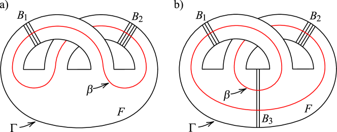
Figure 15. A proper power $\beta$ which intersects each of the bands of $(\partial D_{A}\cup\partial D_{B})\cap F$.

Proof.

Suppose that $\beta$ intersects each of the bands of $(\partial D_{A}\cup\partial D_{B})\cap F$. Then the graph $G(\beta)$ of the Heegaard diagram of $\beta$ with respect to $\{D_{A},D_{B}\}$ omits at most two edges of $G(\Gamma)$, which are invariant under the hyperelliptic involution. See Figure 15, where $\beta$ intersects each of the bands of $(\partial D_{A}\cup\partial D_{B})\cap F$. Since $G(\Gamma)$ is robust, $G(\beta)$ is connected and has no cut-vertex. This is contradiction to Proposition 4.5. ∎

Lemma 5.3.

Suppose that $\beta$ has essential intersections with $\Gamma$. Let $\delta$ be a connection in $\beta\cap F^{\prime}$, and suppose that $\delta$ has been isotoped, keeping its endpoints on $\Gamma$ so $\delta$ has only essential intersections with the bands of $(\partial D_{A}\cup\partial D_{B})\cap F^{\prime}$. Then $\delta$ must be disjoint from one of the bands of $(\partial D_{A}\cup\partial D_{B})\cap F^{\prime}$.

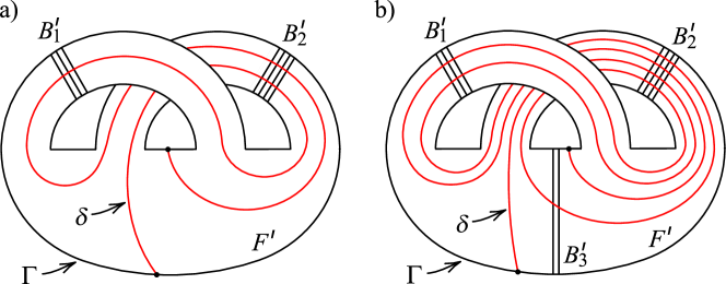
Figure 16. $\delta$ intersects each of the bands of $(\partial D_{A}\cup\partial D_{B})\cap F^{\prime}$ essentially.

Proof.

The proof is similar to that of Proposition 5.2. If $\delta$ intersects each of the bands of $(\partial D_{A}\cup\partial D_{B})\cap F^{\prime}$, then the graph $G(\delta)$ of the Heegaard diagram of $\delta$ with respect to $\{D_{A},D_{B}\}$ omits at most two edges of $G(\Gamma)$. See Figure 16. Since $G(\Gamma)$ is robust, $G(\delta)$ is connected and has no cut-vertex and so is $G(\beta)$, a contradiction. ∎

Let $I=\{1,2\}(\{1,2,3\}$, resp.) when there are two(three, resp.) bands of $(\partial D_{A}\cup\partial D_{B})\cap F^{\prime}$. For $i\in I$, let $|P^{\prime}_{i}|$ denote the number of appearances of ${P^{\prime}_{i}}^{\pm 1}$ in $R$. Note that $R$ can be expressed in terms of the oriented paths $P^{\prime}_{i}$’s as we define $P^{\prime}_{1}{P^{\prime}_{2}}^{-1},P^{\prime}_{1}{P^{\prime}_{3}}^{-1}$, and $P^{\prime}_{2}{P^{\prime}_{3}}^{-1}$ as simple closed curves in $F^{\prime}$. The following proposition describes all possible candidates for $R$ when $\beta$ has an essential intersection with $\Gamma$.

Proposition 5.4.

Suppose that $\beta$ has an essential intersection with $\Gamma$. Then there exists $i_{0}\in I$ such that $|P^{\prime}_{i_{0}}|=1$.

Therefore if there are two bands of $(\partial D_{A}\cup\partial D_{B})\cap F^{\prime}$, then the possible $R$ is of the form $\overline{P^{\prime}}_{i_{0}}$ ${\overline{P^{\prime}}_{j}}^{m}$ for $j\in\{1,2\}$ with $j\neq i_{0}$ and $m\in\mathbb{Z}$.

If there are three bands of $(\partial D_{A}\cup\partial D_{B})\cap F^{\prime}$, the possible $R$ is of the form $P^{\prime}_{i_{0}}{P^{\prime}_{j}}^{-1}(P^{\prime}_{k}{P^{\prime}_{j}}^{-1})^{m}$ for distinct $j,k\in\{1,2,3\}$ with $j,k\neq i_{0}$ and $m\in\mathbb{Z}$.

Proof.

Suppose that $|P^{\prime}_{i}|>1$ for every $i\in I$. Then since any connection $\delta$ of $\beta$ in $F^{\prime}$ is disjoint from $R$, it follows that $\delta$ intersects each of $B_{i}$, $i\in I$, in $F^{\prime}$, which is a contradiction to Lemma 5.3. ∎

6. Application on some P/SF knots

In this section, we give applications of the nonhyperbolic conditions for P/P or P/SF knots demonstrated in the previous sections to some P/SF knots. Consider an abstract R-R diagram of a pair of simple closed curves $(\alpha,M)$ in the boundary of a genus two handlebody $H$ shown in Figure 17 with $p>0$ and $|J|>1$, where $M$ is a meridian of $H[R]$. In other words, $\{M,R\}$ bound a complete set of cutting disks of $H^{\prime}$ such that $(\Sigma;H,H^{\prime})$ is a genus two Heegaard splitting of $S^{3}$ and $R$ is disjoint from $\alpha$. By Theorem 5.1 of [K20c], $H[\alpha]$ is Seifert-fibred over the Möbius band with one exceptional fiber of index $|J|$ and thus $\alpha$ is Seifert in $H$. In addition, since $M\cap\alpha$ is a single point of transverse intersection, $\alpha$ is primitive in $H$. Therefore $\alpha$ is primitive/Seifert.

Lemma 6.1.

All of the knots represented by $\alpha$ in Figure 17 are hyperbolic.

Proof.

Suppose the knot represented by $\alpha$ is not hyperbolic. Then by Theorem 4.1, there exists a proper power curve $\beta$ in $\partial H$ that is disjoint from $R$.

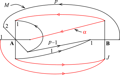
Figure 17. An abstract R-R diagram of a KIST pair $(\alpha,M)$, where $p>0$ and $|J|>1$.

Let $F$ be a regular neighborhood of $\alpha\cup M$ in $\partial H$. Let $\Gamma=\partial F$ and $F^{\prime}=\overline{\partial H-F}$. Then $F$ and $F^{\prime}$ are once-punctured tori with $\Gamma=F\cap F^{\prime}$. Note that $R$ lies completely in $F^{\prime}$. Since $\alpha=A^{-1}B^{J}AB^{J}$ and $M=A(BA^{2})^{p}$ in $\pi_{1}(H)$ when reading from their intersection point, algebraically $\Gamma=M\alpha M^{-1}\alpha^{-1}$ is

$$\Gamma=(A^{2}B)^{p}AB^{J}AB^{J}(A^{-2}B^{-1})^{p}A^{-1}B^{-J}A^{-1}B^{-J}.$$

The R-R diagram of $\Gamma$ when $p=2$ appears as in Figure 18, where some faces which belong to $F$ or $F^{\prime}$ are labelled by the letter $F$ or $F^{\prime}$ respectively. Then $\Gamma$ has a Heegaard diagram $\mathbb{D}_{\Gamma}$ underlying the R-R diagram as illustrated in Figure 19 depending on the sign of $J$.

Figure 18. R-R diagram of $\Gamma$ when $p=2$.

Figure 19. The Heegaard diagram $\mathbb{D}_{\Gamma}$ of $\Gamma$ when $J>1$ in a) and $J<1$ in b) underlying the R-R diagram of $\Gamma$.

It follows that the Heegaard diagram $\mathbb{D}_{\Gamma}$ is robust, and the arcs of $(\partial D_{A}\cup\partial D_{B})\cap F$($(\partial D_{A}\cup\partial D_{B})\cap F^{\prime}$, resp.) cut $F$($F^{\prime}$, resp.) into a number of faces, each of which is a rectangle, except for a pair of hexagonal faces. Therefore $(\partial D_{A}\cup\partial D_{B})\cap F$ and $\partial D_{A}\cup\partial D_{B})\cap F^{\prime}$ consist of three bands of connections in $F$ and $F^{\prime}$ respectively since there are two hexagonal faces in each of $F$ and $F^{\prime}$. Let $Hex_{1}$ and $Hex_{2}$($Hex^{\prime}_{1}$ and $Hex^{\prime}_{2}$, resp.) be the two hexagonal faces in $F$($F^{\prime}$, resp.). They can be obtained in the R-R diagram of $\Gamma$ by isotoping the oriented curves entering into or coming out from the maximally labelled connection in each handle to the oriented curves passing through the other two connections with smaller labels. In the R-R diagram of $\Gamma$, $2$ and $J$ are the maximal labels in the $A$- and $B$-handles respectively. Note that the isotopies in the $B$-handle depend on the sign of $J$. Figures 20a and 20b show the isotopies of the curves passing through the 2-connections and the $J$-connections into the dotted curves passing through the other two connections when $J>1$ and $J<-1$ respectively. With these isotopies performed, we can obtain the hexagonal faces $Hex_{1}$ and $Hex_{2}$ in $F$ and $Hex^{\prime}_{1}$ and $Hex^{\prime}_{2}$ in $F^{\prime}$ as shown in Figure 20.

Figure 20. Hexagonal faces $Hex_{1}$ and $Hex_{2}$ in $F$, and $Hex^{\prime}_{1}$ and $Hex^{\prime}_{2}$ in $F^{\prime}$ when a) $J>1$ and b) $J<-1$.

As discussed in Section 5, we can obtain three oriented paths $P_{1},P_{2},$ and $P_{3}$ from $Hex_{1}$ to $Hex_{2}$ in $F$, whose first homotopies in $\pi_{1}(H)$ are

$$P_{1}=A,\hskip 1.42271ptP_{2}=B^{J}AB^{J},\hskip 4.26773pt\text{and}\hskip 4.55254ptP_{3}=A^{-1}(B^{-1}A^{-2})^{p-1}B^{-1}A^{-1}.$$

Similarly there are three oriented paths $P^{\prime}_{1},P^{\prime}_{2},$ and $P^{\prime}_{3}$ from $Hex^{\prime}_{1}$ to $Hex^{\prime}_{2}$ in $F^{\prime}$, whose first homotopies in $\pi_{1}(H)$ are when $J>1$

$$P^{\prime}_{1}=B^{J-1},\hskip 1.42271ptP^{\prime}_{2}=B^{-1}A^{-1}B^{-J}A^{-1}B^{-1},\hskip 4.26773pt\text{and}\hskip 4.55254ptP^{\prime}_{3}=(A^{2}B)^{p-1}A^{2},$$

and when $J<-1$

$$P^{\prime}_{1}=B^{J+1},\hskip 1.42271ptP^{\prime}_{2}=A^{-1}B^{-J}A^{-1},\hskip 4.26773pt\text{and}\hskip 4.55254ptP^{\prime}_{3}=B(A^{2}B)^{p}.$$

Now we consider the proper power curve $\beta$.

Claim 6.2.

$\beta$ has an essential intersection with $\Gamma$.

Proof.

Suppose $\beta$ has no essential intersections with $\Gamma$, i.e., $\beta\cap\Gamma=\varnothing$. Since $R\subseteq F^{\prime}$, $\beta$ must lie completely in $F$. Since the Heegaard diagram $\mathbb{D}_{\Gamma}$ of $\Gamma$ is robust, by Proposition 5.2, $\beta$ must be one of the curves $P_{1}P_{2}^{-1},P_{1}P_{3}^{-1}$, and $P_{2}P_{3}^{-1}$. It is easy to check that $P_{1}P_{2}^{-1}=\alpha^{-1},P_{1}P_{3}^{-1}=M$. Therefore $\beta=P_{2}P_{3}^{-1}$ whose homotopy is $\beta=B^{J}AB^{J}AB(A^{2}B)^{p-1}A$. If $p>1$, then $A^{2}$ and $B^{J}$ appear, implying that by Proposition 4.6 $\beta$ cannot be a proper power curve. Therefore $p=1$ and $\beta=B^{J}AB^{J}ABA$. The automorphism $A\mapsto B^{-J}A$ sends $\beta$ to $\beta=A^{3}B^{1-J}$, which is not a proper power curve. ∎

By Claim 6.2 $\beta$ has an essential intersection with $\Gamma$. Since $\Gamma$ is robust, by Proposition 5.4 the possible curves for $R$ are the following simple closed curves in $F^{\prime}$ up to orientations:

$$P^{\prime}_{1}{P^{\prime}_{2}}^{-1}(P^{\prime}_{3}{P^{\prime}_{2}}^{-1})^{m},\hskip 1.42271ptP^{\prime}_{2}{P^{\prime}_{1}}^{-1}(P^{\prime}_{3}{P^{\prime}_{1}}^{-1})^{m},\hskip 4.26773pt\text{and}\hskip 4.55254ptP^{\prime}_{3}{P^{\prime}_{2}}^{-1}(P^{\prime}_{1}{P^{\prime}_{2}}^{-1})^{m}$$

where $m\in\mathbb{Z}$, such that when $J>1$,

1. $P^{\prime}_{1}{P^{\prime}_{2}}^{-1}(P^{\prime}_{3}{P^{\prime}_{2}}^{-1})^{m}=B^{J}AB^{J}AB((A^{2}B)^{p-1}A^{2}BAB^{J}AB)^{m}$,

2. $P^{\prime}_{2}{P^{\prime}_{1}}^{-1}(P^{\prime}_{3}{P^{\prime}_{1}}^{-1})^{m}=B^{-1}A^{-1}B^{-J}A^{-1}B^{-J}((A^{2}B)^{p-1}A^{2}B^{-J+1})^{m}$,

3. $P^{\prime}_{3}{P^{\prime}_{2}}^{-1}(P^{\prime}_{1}{P^{\prime}_{2}}^{-1})^{m}=(A^{2}B)^{p-1}A^{2}BAB^{J}AB(B^{J}AB^{J}AB)^{m}$,

and when $J<-1$,

1. $P^{\prime}_{1}{P^{\prime}_{2}}^{-1}(P^{\prime}_{3}{P^{\prime}_{2}}^{-1})^{m}=B^{J+1}AB^{J}A(B(A^{2}B)^{p}AB^{J}A)^{m}$,

2. $P^{\prime}_{2}{P^{\prime}_{1}}^{-1}(P^{\prime}_{3}{P^{\prime}_{1}}^{-1})^{m}=A^{-1}B^{-J}A^{-1}B^{-J-1}(B(A^{2}B)^{p}B^{-J-1})^{m}$,

3. $P^{\prime}_{3}{P^{\prime}_{2}}^{-1}(P^{\prime}_{1}{P^{\prime}_{2}}^{-1})^{m}=B(A^{2}B)^{p}AB^{J}A(B^{J+1}AB^{J}A)^{m}$.

Now we compute the determinant $\Delta=|[M][R]|$, where $[M],[R]\in H_{1}(H)$. $\Delta$ must be unimodular because $H[M,R]\cong S^{3}$. If $J>1$ and $R$ is the curve in the first case (1), i.e., $R=P^{\prime}_{1}{P^{\prime}_{2}}^{-1}(P^{\prime}_{3}{P^{\prime}_{2}}^{-1})^{m}=B^{J}AB^{J}AB((A^{2}B)^{p-1}A^{2}BAB^{J}AB)^{m}$, then

$$\begin{split}|[M][R]|&=\left|\begin{array}[]{cc}2p+1&(2p+2)m+2\\ p&(p+J+1)m+2J+1\\ \end{array}\right|=\left|\begin{array}[]{cc}2p+1&m+2\\ p&(J+1)(m+2)-1\\ \end{array}\right|\\ &=((2p+1)J+p+1)(m+2)-(2p+1).\end{split}$$

The second matrix is obtained from the first matrix by adding $-m$ multiple of the first column to the second column. Similarly we can compute the determinants in the other five cases (2)–(6). All of the determinants $\Delta$ are as follows, where $\Delta_{i}$ denotes the determinant in the case $(i)$ with $i=1,\ldots,6$.

1. $\Delta_{1}=((2p+1)J+p+1)(m+2)-(2p+1)$,

2. $\Delta_{2}=(-(2p+1)J+p)(m+2)-(2p+1)$,

3. $\Delta_{3}=((2p+1)J-p)(2m+1)+(2p+1)(m+1)$,

4. $\Delta_{4}=((2p+1)(J+1)-p)(m+2)-(2p+1)$,

5. $\Delta_{5}=((2p+1)J-p)(m+2)+(2p+1)$,

6. $\Delta_{6}=((2p+1)(J+1)-p)(2m+1)-(2p+1)(m+1)$.

It is easy to see that for all the values of $p,J,$ and $m$ with $p>0$, $|J|>1$, and $m\in\mathbb{Z}$, $\Delta_{i}\neq\pm 1$ for $i=1,\ldots,6$, only except for $\Delta_{4}$ with the set of the parameters $(p,J,m)=(1,-2,-3)$, in which case $\Delta_{4}=1$.

In order to complete the proof, we use Proposition 4.7. Since we have assumed that the knot represented by $\alpha$ is not hyperbolic, $H[R]$ is the exterior of the unknot, a torus knot, or a cable knot. Therefore the curve $R$ can satisfy none of the conditions (1), (2), and (3) in Proposition 4.7, provided that $R$ has at least two bands of connections in each handle. With $(p,J,m)=(1,-2,-3)$ inserted in the case (4), $R$ is

$$\begin{split}R&=B^{-1}AB^{-2}A(BA^{2}BAB^{-2}A)^{-3}\\ &=B^{-3}A^{-2}(B^{-1}A^{-1}B^{2}A^{-1}B^{-1}A^{-2})^{2}.\end{split}$$

Since $A^{-1},A^{-2},B^{-1},B^{2}$ and $B^{-3}$ appear in $R$, $R$ has at least two bands of connections in both the $A$- and $B$-handles. Furthermore, $B^{-3}A^{-2}B^{-1}$ appears in $R$ and thus $R$ satisfies the condition (2) in Proposition 4.7, a contradiction. This completes the proof. ∎

References

- [B20] Berge, J., Distinguished waves and slopes in genus two, preprint.
- [B93] Berge, J., Embedding the Exteriors of One-Tunnel Knots and Links in the 3-Sphere, Unpublished transparencies of invited address at Cascade Topology Conf. Spring 1993.
- [B90] J. Berge, Some Knots with Surgeries Yielding Lens Spaces, Unpublished manuscript. Univ. of Texas at Austin, 1990.
- [B18] Berge, J., Some Knots with Surgeries Yielding Lens Spaces, arXiv preprint arXiv:1802.09722, 2018. original unpublished work from 1990.
- [B08] Berge, J., The simple closed curves in genus two Heegaard surface of which are double-primitives, Unpublished manuscript.
- [BK20] Berge, J. and Kang, S. The hyperbolic primitive/Seifert knots in , preprint.
- [BL89] Bleiler, S. and Litherland, R., Lens spaces and Dehn surgery, P.A.M.S. 107 no. 4, (1989), 1127–1131.
- [BRZ88] Boileau, M., Rost, M., and Zieschang, H., On Heegaard decompositions of torus knot exteriors and related Seifert fibre spaces. Math. Ann. 279 (1988), 553–581.
- [CMZ81] Cohen, M., Metzler, W. and Zimmerman, A., What Does a Basis of F(a,b) Look Like?, Math. Ann. 257 (1981), 435–445.
- [D03] Dean, J., Small Seifert-fibered Dehn surgery on hyperbolic knots, Algebraic and Geometric Topology 3 (2003), 435–472.
- [EM92] Eudave-Muñoz, M., Band sums of links which yield composite links. The cabling conjecture for strongly invertible knots, Trans. Amer. Math. Soc. 330 no. 2, (1992), 463–501.
- [G13] Green, J. E., The lens space realization problem, Ann. of Math. (2) 177 (2013), 449–511.
- [K20a] Kang, S. Hyperbolicity of primitive/primitive knots in , In preparation.
- [K20b] Kang, S. Hyperbolicity of primitive/Seifert knots in , In preparation.
- [K20c] Kang, S. Primitive, proper power, and Seifert curves in the boundary of a genus two handlebody, preprint.
- [K20d] Kang, S. Tunnel-number-one knot exteriors in disjoint from proper power curves, preprint.
- [MM05] Miyazaki, K., and Motegi, K., On primitive/Seifert-fibered constructions, Math. Proc. Camb. Phil. Soc. 138 (2005), 421-435.
- [M88] Moriah, Y., Heegaard splittings of Seifert fibered spaces, Invent. Math., 91 (1988), 465-481.
- [M71] Moser, L., Elementary surgery along a torus knot, Pacific J. Math. 38 (1971) 737–745.
- [MS91] Marimoto, K., and Sakuma, M., On unknotting tunnels for knots, Math. Ann. 289 (1991), 143-167.
- [W36] Whitehead, J. H. C., On Equivalent Sets of Elements in a Free Group, Ann. of Math. 37 (1936), 782–800.
- [W90] Y. Q. Wu, Cyclic surgery and satellite knots, Top. and Apps. 36 no. 3, (1990), 205–208.
- [Z70] Zieschang, H., On Simple Systems of Paths on Complete Pretzel, Amer. Math. Soc. Transl. (2), 92 (1970), 127–137.