Parallel Batch-Dynamic $k$-Clique Counting

Abstract

In this paper, we study new batch-dynamic algorithms for the $k$-clique counting problem, which are dynamic algorithms where the updates are batches of edge insertions and deletions. We study this problem in the parallel setting, where the goal is to obtain algorithms with low (polylogarithmic) depth. Our first result is a new parallel batch-dynamic triangle counting algorithm with $O(\Delta\sqrt{\Delta+m})$ amortized work and $O(\log^{*}(\Delta+m))$ depth with high probability, and $O(\Delta+m)$ space for a batch of $\Delta$ edge insertions or deletions. Our second result is an algebraic algorithm based on parallel fast matrix multiplication. Assuming that a parallel fast matrix multiplication algorithm exists with parallel matrix multiplication constant $\omega_{p}$, the same algorithm solves dynamic $k$-clique counting with $O\left(\min\left(\Delta m^{\frac{(2k-1)\omega_{p}}{3(\omega_{p}+1)}},(\Delta+m)^{\frac{2(k+1)\omega_{p}}{3(\omega_{p}+1)}}\right)\right)$ amortized work and $O(\log(\Delta+m))$ depth with high probability, and $O\left((\Delta+m)^{\frac{2(k+1)\omega_{p}}{3(\omega_{p}+1)}}\right)$ space. Using a recently developed parallel $k$-clique counting algorithm, we also obtain a simple batch-dynamic algorithm for $k$-clique counting on graphs with arboricity $\alpha$ running in $O(\Delta(m+\Delta)\alpha^{k-4})$ expected work and $O(\log^{k-2}n)$ depth with high probability, and $O(m+\Delta)$ space. Finally, we present a multicore CPU implementation of our parallel batch-dynamic triangle counting algorithm. On a 72-core machine with two-way hyper-threading, our implementation achieves 36.54–74.73x parallel speedup, and in certain cases achieves significant speedups over existing parallel algorithms for the problem, which are not theoretically-efficient.

1 Introduction

Subgraph counting algorithms are fundamental graph analysis tools, with numerous applications in network classification in domains including social network analysis and bioinformatics. A particularly important type of subgraph for these applications is the triangle, or $3$-clique—three vertices that are all mutually connected [New03]. Counting the number of triangles is a basic and fundamental task that is used in numerous social and network science measurements [Gra77, WS98].

In this paper, we study the triangle counting problem and its generalization to higher cliques from the perspective of dynamic algorithms. A $k$-clique consists of $k$ vertices and all $k\choose{2}$ possible edges among them (for applications of $k$-cliques, see, e.g., [HR05]). As many real-world graphs change rapidly in real-time, it is crucial to design dynamic algorithms that efficiently maintain $k$-cliques upon updates, since the cost of re-computation from scratch can be prohibitive. Furthermore, due to the fact that dynamic updates can occur at a rapid rate in practice, it is increasingly important to design batch-dynamic algorithms which can take arbitrarily large batches of updates (edge insertions or deletions) as their input. Finally, since the batches, and corresponding update complexity can be large, it is also desirable to use parallelism to speed-up maintenance and design algorithms that map to modern parallel architectures.

Due to the broad applicability of $k$-clique counting in practice and the fact that $k$-clique counting is a fundamental theoretical problem of its own right, there has been a large body of prior work on the problem. Theoretically, the fastest static algorithm for arbitrary graphs uses fast matrix multiplication, and counts $3\ell$ cliques in $O(n^{\ell\omega})$ time where $\omega$ is the matrix multiplication exponent [NP85]. Considerable effort has also been devoted to efficient combinatorial algorithms. Chiba and Nishizeki [CN85] show how to compute $k$-cliques in $O(\alpha^{k-2}m)$ work, where $m$ is the number of edges in the graph and $\alpha$ is the arboricity of the graph. This algorithm was recently parallelized by Danisch et al. [DBS18a] (although not in polylogarithmic depth). Worst-case optimal join algorithms can perform $k$-clique counting in $O(m^{k/2})$ work as a special case [NPRR18, ALT⁺17]. Alon, Yuster, and Zwick [AYZ97] design an algorithm for triangle counting in the sequential model, based on fast matrix multiplication. Eisenbrand and Grandoni [EG04] then extend this result to $k$-clique counting based on fast matrix multiplication. Vassilevska designs a space-efficient combinatorial algorithm for $k$-clique counting [Vas09]. Finocchi et al.  give clique counting algorithms for MapReduce [FFF15]. Jain and Seshadri provide probabilistic algorithms for estimating clique counts [JS17]. The $k$-clique problem is also a classical problem in parameterized-complexity, and is known to be $W[1]$-complete [DF95].

The problem of maintaining $k$-cliques under dynamic updates began more recently. Eppstein et al. [ES09, EGST12] design sequential dynamic algorithms for maintaining size-3 subgraphs in $O(h)$ amortized time and $O(mh)$ space and size-4 subgraphs in $O(h^{2})$ amortized time and $O(mh^{2})$ space, where $h$ is the $h$-index of the graph ($h=O(\sqrt{m})$). Ammar et al. extend the worst-case optimal join algorithms to the parallel and dynamic setting [AMSJ18]. However, their update time is not better than the static worst-case optimal join algorithm. Recently, Kara et al. [KNN⁺19] present a sequential dynamic algorithm for maintaining triangles in $O(\sqrt{m})$ amortized time and $O(m)$ space. Dvorak and Tuma [DT13] present a dynamic algorithm that maintains $k$-cliques as a special case in $O(\alpha^{k-2}\log n)$ amortized time and $O(\alpha^{k-2}m)$ space by using low out-degree orientations for graphs with arboricity $\alpha$.

Designing Parallel Batch-Dynamic Algorithms. Traditional dynamic algorithms receive and apply updates one at a time. However, in the parallel batch-dynamic setting, the algorithm receives batches of updates one after the other, where each batch contains a mix of edge insertions and deletions. Unlike traditional dynamic algorithms, a parallel batch-dynamic algorithm can apply all of the updates together, and also take advantage of parallelism while processing the batch. We note that the edges inside of a batch may also be ordered (e.g., by a timestamp). If there are duplicate edge insertions within a batch, or an insertion of an edge followed by its deletion, a batch-dynamic algorithm can easily remove such redundant or nullifying updates.

The key challenge is to design the algorithm so that updates can be processed in parallel while ensuring low work and depth bounds. The only existing parallel batch-dynamic algorithms for $k$-clique counting are triangle counting algorithms by Ediger et al. [EJRB10] and Makkar et al. [MBG17], which take linear work per update in the worst case. The algorithms in this paper make use of efficient data structures such as parallel hash tables, which let us perform parallel batches of edge insertions and deletions with better work and (polylogarithmic) depth bounds. To the best of our knowledge, no prior work has designed dynamic algorithms for the problem that support parallel batch updates with non-trivial theoretical guarantees.

Theoretically-efficient parallel dynamic (and batch-dynamic) algorithms have been designed for a variety of other graph problems, including minimum spanning tree [KPR18, FL94, DF94], Euler tour trees [TDB19], connectivity [STTW18, AABD19, FL94], tree contraction [RT94, AAW17], and depth-first search [Kha17]. Very recently, parallel dynamic algorithms were also designed for the Massively Parallel Computation (MPC) setting [ILMP19, DDK⁺20].

Other Related Work. There has been significant amount of work on practical parallel algorithms for the case of static 3-clique counting, also known as triangle counting. (e.g., [SV11, AKM13, PC13, PSKP14, ST15], among many others). Due to the importance of the problem, there is even an annual competition for parallel triangle counting solutions [Gra]. Practical static counting algorithms for the special cases of $k=4$ and $k=5$ have also been developed [HD14, ESBD16, PSV17, ANR⁺17, DAH17].

Dynamic algorithms have been studied in distributed models of computation under the framework of self-stabilization [Sch93]. In this setting, the system undergoes various changes, for example topology changes, and must quickly converge to a stable state. Most of the existing work in this setting focuses on a single change per round [CHHK16, BCH19, AOSS19], although algorithms studying multiple changes per round have been considered very recently [BKM19, CHDK⁺19]. Understanding how these algorithms relate to parallel batch-dynamic algorithms is an interesting question for future work.

Summary of Our Contributions. In this paper, we design parallel algorithms in the batch-dynamic setting, where the algorithm receives a batch of $\Delta\geq 1$ edge updates that can be processed in parallel. Our focus is on parallel batch-dynamic algorithms that admit strong theoretical bounds on their work and have polylogarithmic depth with high probability. Note that although our work bounds may be amortized, our depth will be polylogarithmic with high probability, leading to efficient $\mathsf{RNC}$ algorithms. As a special case of our results, we obtain algorithms for parallelizing single updates ($\Delta=1$). We first design a parallel batch-dynamic triangle counting algorithm based on the sequential algorithm of Kara et al. [KNN⁺19]. For triangle counting, we obtain an algorithm that takes $O(\Delta\sqrt{\Delta+m})$ amortized work and $O(\log^{*}(\Delta+m))$ depth w.h.p. assuming a fetch-and-add instruction that runs in $O(1)$ work and depth, and runs in $O(\Delta+m)$ space. The work of our parallel algorithm matches that of the sequential algorithm of performing one update at a time (i.e., it is work-efficient), and we can perform all updates in parallel with low depth.

We then present a new parallel batch-dynamic algorithm based on fast matrix multiplication. Using the best currently known parallel matrix multiplication [Wil12, LG14], our algorithm dynamically maintains the number of $k$-cliques in $O\left(\min\left(\Delta m^{0.469k-0.235},(\Delta+m)^{0.469k+0.469}\right)\right)$ amortized work w.h.p. per batch of $\Delta$ updates where $m$ is defined as the maximum number of edges in the graph before and after all updates in the batch are applied. Our approach is based on the algorithm of [AYZ97, EG04, NP85], and maintains triples of $k/3$-cliques that together form $k$-cliques. The depth is $O(\log(\Delta+m))$ w.h.p. and the space is $O\left((\Delta+m)^{0.469k+0.469}\right)$. Our results also imply an amortized time bound of $O\left(m^{0.469k-0.235}\right)$ per update for dense graphs in the sequential setting. Of potential independent interest, we present the first proof of logarithmic depth in the parallelization of any tensor-based fast matrix multiplication algorithms. We also give a simple batch-dynamic $k$-clique listing algorithm, based on enumerating smaller cliques and intersecting them with edges in the batch. The algorithm runs in $O(\Delta(m+\Delta)\alpha^{k-4})$ expected work, $O(\log^{k-2}n)$ depth w.h.p., and $O(m+\Delta)$ space.

Finally, we implement our new parallel batch-dynamic triangle counting algorithm for multicore CPUs, and present some experimental results on large graphs and with varying batch sizes using a 72-core machine with two-way hyper-threading. We found our parallel implementation to be much faster than the multicore implementation of Ediger et al. [EJRB10]. We also developed an optimized multicore implementation of the GPU algorithm by Makkar et al. [MBG17]. We found that our new algorithm is up to an order of magnitude faster than our CPU implementation of the Makkar et al. algorithm, and our new algorithm achieves 36.54–74.73x parallel speedup on 72 cores with hyper-threading. Our code is publicly available at https://github.com/ParAlg/gbbs.

2 Preliminaries

Given an undirected graph $G=(V,E)$ with $n$ vertices and $m$ edges, and an integer $k$, a $k$-clique is defined as a set of $k$ vertices $v_{1},\ldots,v_{k}$ such that for all $i\neq j$, $(v_{i},v_{j})\in E$. The $k$-clique count is the total number of $k$-cliques in the graph. The dynamic $k$-clique problem maintains the number of $k$-cliques in the graph upon edge insertions and deletions, given individually or in a batch. The arboricity $\alpha$ of a graph is the minimum number of forests that the edges can be partitioned into and its value is between $\Omega(1)$ and $O(\sqrt{m})$ [CN85].

In this paper, we analyze algorithms in the work-depth model, where the work of an algorithm is defined to be the total number of operations done, and the depth is defined to be the longest sequential dependence in the computation (or the computation time given an infinite number of processors) [Jaj92]. Our algorithms can run in the PRAM model or the fork-join model with arbitrary forking. We use the concurrent-read concurrent-write (CRCW) model, where reads and writes to a memory location can happen concurrently. We assume either that concurrent writes are resolved arbitrarily, or are reduced together (i.e., fetch-and-add PRAM).

We use the following primitives throughout the paper. Approximate compaction takes a set of $m$ objects in the range $[1,n]$ and allocates them unique IDs in the range $[1,O(m)]$. The primitive is useful for filtering (i.e., removing) out a set of obsolete elements from an array of size $n$, and mapping the remaining $m$ elements to a sparse array of size $O(m)$. Approximate compaction can be implemented in $O(n)$ work and $O(\log^{*}n)$ depth w.h.p. [GMV91]. We also use a parallel hash table which supports $n$ operations (insertions, deletions) in $O(n)$ work and $O(\log^{*}n)$ depth w.h.p., and $n$ lookup operations in $O(n)$ work and $O(1)$ depth [GMV91].

Our algorithms in this paper make use of the widely used atomic-add instruction. An atomic-add instruction takes a memory location and atomically increments the value stored at the location. In this paper, we assume that the atomic-add instruction can be implemented in $O(1)$ work and depth. Our algorithms can also be implemented in a model without atomic-add in the same work, a multiplicative $O(\log n)$ factor increase in the depth, and space proportional to the number of atomic-adds done in parallel.

3 Technical Overview

In this section, we present a high-level technical overview of our approach in this paper.

3.1 Parallel Batch-Dynamic Triangle Counting

Our parallel batch-dynamic triangle counting algorithm is based on a recently proposed sequential dynamic algorithm due to Kara et al. [KNN⁺19]. They describe their algorithm in the database setting, in the context of dynamically maintaining the result of a database join. We provide a self-contained description of their sequential algorithm in Appendix A.

High-Level Approach. The basic idea of the algorithm from [KNN⁺19] is to partition the vertex set using degree-based thresholding. Roughly, they specify a threshold $t=\Theta(\sqrt{m})$, and classify all vertices with degree less than $t$ to be low-degree, and all vertices with degree larger than $t$ to be high-degree. This thresholding technique is widely used in the design of fast static triangle counting and $k$-clique counting algorithms, (e.g., [NP85, AYZ97]). Observe that if we insert an edge $(u,v)$ incident to a low-degree vertex, $u$, we can enumerate all vertices $w$ in $N(u)$ in $O(\sqrt{m})$ expected time and check if $(u,v,w)$ forms a triangle (checking if the $(v,w)$ edge is present in $G$ can be done by storing all edges in a hash table). In this way, edge updates incident to low-degree vertices are handled relatively simply. The more interesting case is how to handle edge updates between high-degree vertices. The main problem is that a single edge insertion $(u,v)$ between two high-degree vertices can cause up to $O(n)$ triangles to appear in $G$, and enumerating all of these would require $O(n)$ work—potentially much more than $O(\sqrt{m})$. Therefore, the algorithm maintains an auxiliary data structure, $\mathcal{T}$, over wedges ($2$-paths). $\mathcal{T}$ stores for every pair of high-degree vertices $(v,w)$, the number of low-degree vertices $u$ that are connected to both $v$ and $w$ (i.e., $(u,v)$ and $(u,w)$ are both in $E$). Given this structure, the number of triangles formed by the insertion of the edge $(v,w)$ going between two high-degree vertices can be found in $O(1)$ time by checking the count for $(v,w)$ in $\mathcal{T}$. Updates to $\mathcal{T}$ can be handled in $O(\sqrt{m})$ time, since $\mathcal{T}$ need only be updated when a low-degree vertex inserts/deletes a neighbor, and the number of entries in $\mathcal{T}$ that are affected is at most $t$. Some additional care needs to be taken when specifying the threshold $t$ to handle re-classifying vertices (going from low-degree to high-degree, or vice versa), and also to handle rebuilding the data structures, which leads to a bound of $O(\sqrt{m})$ amortized work per update for the algorithm.

Incorporating Batching and Parallelism. The input to the parallel batch-dynamic algorithm is a batch containing (possibly) a mix of edge insertions and deletions (vertex insertions and deletions can be handled by inserting or deleting its incident edges). For simplicity, and without any loss in our asymptotic bounds, our algorithm handles insertions and deletions separately. The algorithm first removes all nullifying updates, which are updates that have no effect after applying the entire batch (i.e., an insertion which is subsequently deleted within the same batch, an insertion of an edge that already exists or a deletion of an edge that doesn’t exist). This can easily be done within the bounds using basic parallel primitives. The algorithm then updates tables representing the adjacency information of both low-degree and high-degree vertices in parallel. To obtain strong parallel bounds, we represent these sets using parallel hash tables. For each insertion (deletion), we then determine the number of new triangles that are created (deleted). Since a given triangle could incorporate multiple edges within the same batch of insertions (deletions), our algorithm must carefully ensure that the triangle is counted only once, assigning each new inserted (deleted) triangle uniquely to one of the updates forming it. We then update the overall triangle count with the number of distinct triangles inserted (deleted) into the graph by the current batch of insertions (deletions). The remaining work of the algorithm cleans up mutable state in the hash tables, and also migrates vertices between low-degree and high-degree states.

Worst-Case Optimality. Our work bounds match the combinatorial lower bound obtained via a fine-grained reduction from triangle detection which is conjectured to take $m^{3/2-o(1)}$ work (by the Strong Triangle conjecture of [AW14] for combinatorial algorithms). The combinatorial lower bound for the Strong Triangle conjecture is based on the standard lower bound conjecture for combinatorial algorithms that solve Boolean Matrix Multiplication (BMM). Our reduction proceeds as follows. Given any input graph to the triangle detection problem, we divide the edges into batches of edge insertions arbitrarily without knowledge of the existence of (any) triangles. Then, the batches of updates are applied one after the other. Suppose the amortized work per update for this procedure is $O(X)$. Then, the total work for applying all the batches of updates is $O(Xm)$. The algorithm returns the count of the number of triangles in the graph after applying all batches of updates. In this case, the algorithm when run over all the batches solves the static problem of triangle detection in the original input graph. If the number of triangles counted by the algorithm after the last batch is $0$, then there does not exist a triangle in the original input graph; otherwise, there exists a triangle in the original input graph. If $X=m^{1/2-\Omega(1)}$, then we violate the Strong Triangle conjecture. Thus, our work bound is conditionally optimal up to sub-polynomial factors by the Strong Triangle conjecture.

It is an interesting open question to consider whether one can obtain $O(1)$ depth bounds on the CRCW PRAM.

3.2 Dynamic $k$-Clique Counting via Fast Static Parallel Algorithms

Next, we present a very simple, and potentially practical algorithm for dynamically maintaining the number of $k$-cliques based on statically enumerating smaller cliques in the graph, and intersecting the enumerated cliques with the edge updates in the input batch. The algorithm is space-efficient, and is asymptotically more efficient than other methods for sparse graphs. Our algorithm is based on a recent and concurrent work proposing a work-efficient parallel algorithm for counting $k$-cliques in $O(m\alpha^{k-2})$ expected work and polylogarithmic depth w.h.p. [SDS20]. Using this algorithm, we show that updating the $k$-clique count for a batch of $\Delta$ updates can be done in $O(\Delta(m+\Delta)\alpha^{k-4})$ expected work, and $O(\log^{k-2}n)$ depth w.h.p., using $O(m+\Delta)$ space. We do this by using the static algorithm to (i) enumerate all $(k-2)$-cliques, and (ii) checking whether each $(k-2)$-clique forms a $k$-clique with an edge in the batch.

3.3 Dynamic $k$-Clique via Fast Matrix Multiplication

We then present a parallel batch-dynamic $k$-clique counting algorithm using parallel fast matrix multiplication (MM). Our algorithm is inspired by the static triangle counting algorithm of Alon, Yuster, and Zwick (AYZ) [AYZ97] and the static $k$-clique counting algorithm of [EG04] that uses MM-based triangle counting. We present a new batch-dynamic algorithm that obtains better bounds than the simple algorithm based on static smaller-clique enumeration above (and also presented in Section 5) for $k>9$. To the best of our knowledge, this is also the best bound for dynamic triangle counting on dense graphs in the sequential model. Specifically, assuming a parallel matrix multiplication exponent of $\omega_{p}$, our algorithm handles batches of $\Delta$ edge insertions/deletions using $O\left(\min\left(\Delta m^{\frac{(2k-3)\omega_{p}}{3(1+\omega_{p})}},(m+\Delta)^{\frac{2k\omega_{p}}{3(1+\omega_{p})}}\right)\right)$ work and $O(\log m)$ depth w.h.p., in $O\left((m+\Delta)^{\frac{2k\omega_{p}}{3(1+\omega_{p})}}\right)$ space, where $m$ is the number of edges in the graph before applying the batch of updates. To the best of our knowledge, the sequential (batch-dynamic) version of our algorithm also provides the best bounds for dynamic triangle counting in the sequential model for dense graphs for such values of $k$ (assuming that we use the best currently known matrix multiplication algorithm) [DT13].

High-Level Approach and Techniques. For a given graph $G=(V,E)$, we create an auxiliary graph $G^{\prime}=(V^{\prime},E^{\prime})$ with vertices and edges representing cliques of various sizes in $G$. For a given $k$-clique problem, vertices in $V^{\prime}$ represent cliques of size $k/3$ in $G$ and edges $(u,v)$ between vertices $u,v\in V^{\prime}$ represent cliques of size $2k/3$ in $G$. Thus, a triangle in $G^{\prime}$ represents a $k$-clique in $G$. Specifically, there exists exactly ${k\choose k/3}{2k/3\choose k/3}$ different triangles in $G^{\prime}$ for each clique in $G$.

Given a batch of edge insertions and deletions to $G$, we create a set of edge insertions and deletions to $G^{\prime}$. An edge is inserted in $G^{\prime}$ when a new $2k/3$-clique is created in $G$ and an edge is deleted in $G^{\prime}$ when a $2k/3$-clique is destroyed in $G$. Suppose, for now, that we have a dynamic algorithm for processing the edge insertions/deletions into $G^{\prime}$. Counting the number of triangles in $G^{\prime}$ after processing all edge insertions/deletions and dividing by ${k\choose k/3}{2k/3\choose k}$ provides us with the exact number of cliques in $G$.

There are a number of challenges that we must deal with when formulating our dynamic triangle counting algorithm for counting the triangles in $G^{\prime}$:

1. We cannot simply count all the triangles in $G^{\prime}$ after inserting/deleting the new edges as this does not perform better than a trivial static algorithm.

2. Any trivial dynamization of the AYZ algorithm will not be able to detect all new triangles in $G^{\prime}$. Specifically, because the AYZ algorithm counts all triangles containing a low-degree vertex separately from all triangles containing only high-degree vertices, if an edge update only occurs between high-degree vertices, a trivial dynamization of the algorithm will not be able to detect any triangle that the two high-degree endpoints make with low-degree vertices.

To solve the first challenge, we dynamically count low-degree and high-degree vertices in different ways. Let $\ell=k/3$ and $M=2m+1$. For some value of $0<t<1$, we define low-degree vertices to be vertices that have degree less than $M^{t\ell}/2$ and high-degree vertices to have degree greater than $3M^{t\ell}/2$. Vertices with degrees in the range $[M^{t\ell}/2,3M^{t\ell}/2]$ can be classified as either low-degree or high-degree. We determine the specific value for $t$ in Lemma 6.12. We perform rebalancing of the data structures as needed as they handle more updates. For low-degree vertices, we only count the triangles that include at least one newly inserted/deleted edge, at least one of whose endpoints is low-degree. This means that we do not need to count any pre-existing triangles that contain at least one low-degree vertex. For the high-degree vertices, because there is an upper bound on the maximum number of such vertices in the graph, we update an adjacency matrix $A$ containing only edges between high-degree vertices. At the end of all of the edge updates, computing $A^{3}$ gives us a count of all of the triangles that contain three high-degree vertices.

This procedure immediately then leads to our second challenge. To solve this second challenge, we make the observation (proven in Lemma 6.3) that if there exists an edge update between two high-degree vertices that creates or destroys a triangle that contains a low-degree vertex in $G^{\prime}$, then there must exist at least one new edge insertion/deletion that creates or destroys a triangle representing the same clique to that low-degree vertex in the same batch of updates to $G^{\prime}$. Thus, we can use one of those edge insertions/deletions to determine the new clique that was created and, through this method, find all triangles containing at least one low-degree vertex and at least one new edge update. Some care must be observed in implementing this procedure in order to not increase the runtime or space usage; such details can be found in Section 6.2.

Incorporating Batching and Parallelism. When dealing with a batch of updates containing both edge insertions and deletions, we must be careful when vertices switch from being high-degree to being low-degree, and vice versa. If we intersperse the edge insertions with the edge deletions, there is the possibility that a vertex switches between low and high-degree multiple times in a single batch. Thus, we batch all edge deletions together and perform these updates first before handling the edge insertions. After processing the batch of edge deletions, we must subsequently move any high-degree vertices that become low-degree to their correct data structures. After dealing with the edge insertions, we must similarly move any low-degree vertices that become high-degree to the correct data structures. Finally, for triangles that contain more than one edge update, we must account for potential double counting by different updates happening in parallel. Such challenges are described and dealt with in Section 6.2 and Algorithm 6.3.

3.4 Implementation and Experimental Evaluation

We present an optimized implementation of our new parallel batch-dynamic triangle counting algorithm using parallel primitives from the Graph Based Benchmark Suite (GBBS) [DBS18b], and concurrent hash tables [SB14] to represent our data structures. We ran experiments on varying batch sizes for both insertions and deletions for several large graphs (the Orkut and Twitter graphs, as well as rMAT graphs of varying densities) using a 72-core machine with two-way hyper-threading, and obtained parallel speedups of between 36.54–74.73x. We also compared our performance to the algorithms by Ediger et al. [EJRB10] and Makkar et al. [MBG17] (we note that Makkar et al. provide a GPU implementation, and we implemented a multicore CPU version of their algorithm), which take linear work per update in the worst case. We found that our Makkar et al. implementation outperformed the multicore implementation by Ediger et al. Furthermore, our new algorithm achieves significant speedups (up to an order of magnitude) over the Makkar et al. implementation on graphs with high-degree vertices (the Twitter graph and dense rMAT graphs), as well as on smaller batch sizes. In contrast, the Makkar et al. implementation outperforms our new algorithm for the smaller Orkut graph, which does not contain vertices with very high degree. These results are consistent with the theoretical bounds of the algorithms—the work per update of our algorithm is $O(\sqrt{m})$, whereas the work per update of the Makkar et al. algorithm is linear in the degrees of the affected vertices.

4 Parallel Batch-Dynamic Triangle Counting

We now present our parallel batch-dynamic triangle counting algorithm, which is based on the $O(m)$ space and $O(\sqrt{m})$ amortized update, sequential, dynamic algorithm of Kara et al. [KNN⁺19]. Theorem 4.1 summarizes the guarantees of our algorithm.

Theorem 4.1.

There exists a parallel batch-dynamic triangle counting algorithm that requires $O(\Delta(\sqrt{\Delta+m}))$ amortized work and $O(\log^{*}(\Delta+m))$ depth with high probability, and $O(\Delta+m)$ space for a batch of $\Delta$ edge updates.

Our algorithm is work-efficient and achieves a significantly lower depth for a batch of updates than applying the updates one at a time using the sequential algorithm of [KNN⁺19]. We provide a detailed description of the fully dynamic sequential algorithm of [KNN⁺19] in Appendix A for reference, and a brief high-level overview of that algorithm in this section.

4.1 Sequential Algorithm Overview

Given a graph $G=(V,E)$ with $n=|V|$ vertices and $m=|E|$ edges, let $M=2m+1$, $t_{1}=\sqrt{M}/2$, and $t_{2}=3\sqrt{M}/2$. We classify a vertex as low-degree if its degree is at most $t_{1}$ and high-degree if its degree is at least $t_{2}$. Vertices with degree in between $t_{1}$ and $t_{2}$ can be classified either way.

Data Structures. The algorithm partitions the edges into four edge-stores $\mathcal{HH}$, $\mathcal{HL}$, $\mathcal{LH}$, and $\mathcal{LL}$ based on a degree-based partitioning of the vertices. $\mathcal{HH}$ stores all of the edges $(u,v)$, where both $u$ and $v$ are high-degree. $\mathcal{HL}$ stores edges $(u,v)$, where $u$ is high-degree and $v$ is low-degree. $\mathcal{LH}$ stores the edges $(u,v)$, where $u$ is low-degree and $v$ is high-degree. Finally, $\mathcal{LL}$ stores edges $(u,v)$, where both $u$ and $v$ are low-degree.

The algorithm also maintains a wedge-store $\mathcal{T}$ (a wedge is a triple of distinct vertices $(x,y,z)$ where both $(x,y)$ and $(y,z)$ are edges in $E$). For each pair of high-degree vertices $u$ and $v$, the wedge-store $\mathcal{T}$ stores the number of wedges $(u,w,v)$, where $w$ is a low-degree vertex. $\mathcal{T}$ has the property that given an edge insertion (resp. deletion) $(u,v)$ where both $u$ and $v$ are high-degree vertices, it returns the number of wedges $(u,w,v)$, where $w$ is low-degree, that $u$ and $v$ are part of in $O(1)$ expected time. $\mathcal{T}$ is implemented via a hash table indexed by pairs of high-degree vertices that stores the number of wedges for each pair.

Finally, we have an array containing the degrees of each vertex, $\mathcal{D}$.

Initialization. Given a graph with $m$ edges, the algorithm first initializes the triangle count $C$ using a static triangle counting algorithm in $O(\alpha m)=O(m^{3/2})$ work and $O(m)$ space [Lat08]. The $\mathcal{HH}$, $\mathcal{HL}$, $\mathcal{LH}$, and $\mathcal{LL}$ tables are created by scanning all edges in the input graph and inserting them into the appropriate hash tables. $\mathcal{T}$ can be initialized by iterating over edges $(u,w)$ in $\mathcal{HL}$ and for each $w$, iterating over all edges $(w,v)$ in $\mathcal{LH}$ to find pairs of high-degree vertices $u$ and $v$, and then incrementing $\mathcal{T}(u,v)$.

The Kara et al. Algorithm [KNN⁺19]. Given an edge insertion $(u,v)$ (deletions are handled similarly, and for simplicity assume that the edge does not already exist in $G$), the update algorithm must identify all tuples $(u,w,v)$ where $(u,w)$ and $(v,w)$ already exist in $G$, since such triples correspond to new triangles formed by the edge insertion. The algorithm proceeds by considering how a triangle’s edges can reside in the data structures. For example, if all of $u$, $v$, and $w$ are high-degree, then the algorithm will enumerate these triangles by checking $\mathcal{HH}$ and finding all neighbors $w$ of $u$ that are also high-degree (there are at most $O(\sqrt{m})$ such neighbors), checking if the $(v,w)$ edge exists in constant time. On the other hand, if $u$ is low-degree, then checking its $O(\sqrt{m})$ many neighbors suffices to enumerate all new triangles. The interesting case is if both $u$ and $v$ are high-degree, but $w$ is low-degree, since there can be much more than $O(\sqrt{m})$ such $w$’s. This case is handled using $\mathcal{T}$, which stores for a given $(u,v)$ edge in $\mathcal{HH}$ all $w$ such that $(w,u)$ and $(w,v)$ both exist in $\mathcal{LH}$.

Finally, the algorithm updates the data structures, first inserting the new edge into the appropriate edge-store. The algorithm updates $\mathcal{T}$ as follows. If $u$ and $v$ are both low-degree or both high-degree, then no update is needed to $\mathcal{T}$. Otherwise, without loss of generality suppose $u$ is low-degree and $v$ is high-degree. Then, the algorithm enumerates all high-degree vertices $w$ that are neighbors of $u$ and increments the value of $(v,w)$ in $\mathcal{T}$.

4.2 Parallel Batch-Dynamic Update Algorithm

We present a high-level overview of our parallel algorithm in this section, and a more detailed description in Section 4.3. We consider batches of $\Delta$ edge insertions and/or deletions. Let $\mathtt{insert}(u,v)$ represent the update corresponding to inserting an edge between vertices $u$ and $v$, and $\mathtt{delete}(u,v)$ represent deleting the edge between $u$ and $v$. We first preprocess the batch to account for updates that nullify each other. For example, an $\mathtt{insert}(u,v)$ update followed chronologically by a $\mathtt{delete}(u,v)$ update nullify each other because the $(u,v)$ edge that is inserted is immediately deleted, resulting in no change to the graph. To process the batch consisting of nullifying updates, we claim that the only update that is not nullifying for any pair of vertices is the chronologically last update in the batch for that edge. Since all updates contain a timestamp, to account for nullifying updates we first find all updates on the same edge by hashing the updates by the edge that it is being performed on. Then, we run the parallel maximum-finding algorithm given in [Vis10] on each set of updates for each edge in parallel. This maximum-finding algorithm then returns the update with the largest timestamp (the most recent update) from the set of updates for each edge. This set of returned updates then composes a batch of non-nullifying updates.

Before we go into the details of our parallel batch-dynamic triangle counting algorithm, we first describe some challenges that must be solved in using Kara et al. [KNN⁺19] for the parallel batch-dynamic setting.

Challenges. Because Kara et al. [KNN⁺19] only considers one update at a time in their algorithm, they do not deal with cases where a set of two or more updates creates a new triangle. Since, in our setting, we must account for batches of multiple updates, we encounter the following set of challenges:

1. We must be able to efficient find new triangles that are created via two or more edge insertions.

2. We must be able to handle insertions and deletions simultaneously meaning that a triangle with one inserted edge and one deleted edge should not be counted as a new triangle.

3. We must account for over-counting of triangles due to multiple updates occurring simultaneously.

For the rest of this section, we assume that $\Delta\leq m$, as otherwise we can re-initialize our data structure using the static parallel triangle-counting algorithm [ST15] to get the count in $O(\Delta^{3/2})$ work, $O(\log^{*}\Delta)$ depth, and $O(\Delta)$ space (assuming atomic-add), which is within the bounds of Theorem 4.1.

Parallel Initialization. Given a graph with $m$ edges, we initialize the triangle count $C$ using a static parallel triangle counting algorithm in $O(\alpha m)=O(m^{3/2})$ work, $O(\log^{*}m)$ depth, and $O(m)$ space [ST15], using atomic-add. We initialize $\mathcal{HH}$, $\mathcal{HL}$, $\mathcal{LH}$, and $\mathcal{LL}$ by scanning the edges in parallel and inserting them into the appropriate parallel hash tables. We initialize the degree array $\mathcal{D}$ by scanning the vertices. Both steps take $O(m)$ work and $O(\log^{*}m)$ depth w.h.p. $\mathcal{T}$ can be initialized by iterating over edges $(u,w)$ in $\mathcal{HL}$ in parallel and for each $w$, iterating over all edges $(w,v)$ in $\mathcal{LH}$ in parallel to find pairs of high-degree vertices $u$ and $v$, and then incrementing $\mathcal{T}(u,v)$. The number of entries in $\mathcal{HL}$ is $O(m)$ and each $w$ has $O(\sqrt{m})$ neighbors in $\mathcal{LH}$, giving a total of $O(m^{3/2})$ work and $O(\log^{*}m)$ depth w.h.p. for the hash table insertions. The amortized work per edge update is $O(\sqrt{m})$.

Data Structure Modifications. We now describe additional information that is stored in $\mathcal{HH}$, $\mathcal{HL}$, $\mathcal{LH}$, $\mathcal{LL}$, and $\mathcal{T}$, which is used by the batch-dynamic update algorithm:

1. Every edge stored in $\mathcal{HH}$, $\mathcal{HL}$, $\mathcal{LH}$, and $\mathcal{LL}$ stores an associated state, indicating whether it is an old edge, a new insertion or a new deletion, which correspond to the values of 0, 1, and 2, respectively.

2. $\mathcal{T}(u,v)$ stores a tuple with 5 values instead of a single value for each index $(u,v)$. Specifically, a $5$-tuple entry of $\mathcal{T}(u,v)=(t^{(u,v)}_{1},t^{(u,v)}_{2},t^{(u,v)}_{3},t^{(u,v)}_{4},t^{(u,v)}_{5})$ represents the following:

   • $t^{(u,v)}_{1}$ represents the number of wedges with endpoints $u$ and $v$ that include only old edges.

   • $t^{(u,v)}_{2}$ and $t^{(u,v)}_{3}$ represent the number of wedges with endpoints $u$ and $v$ containing one or two newly inserted edges, respectively.

   • $t^{(u,v)}_{4}$ and $t^{(u,v)}_{5}$ represent the number of wedges with endpoints $u$ and $v$ containing one or two newly deleted edges, respectively. In other words, they are wedges that do not exist anymore due to one or two edge deletions.

Algorithm Overview. We first remove updates in the batch that either insert edges already in the graph or delete edges not in the graph by using approximate compaction to filter. Next, we update the tables $\mathcal{HH}$, $\mathcal{HL}$, $\mathcal{LH}$, and $\mathcal{LL}$ with the new edge insertions. Recall that we must update the tables with both $(u,v)$ and $(v,u)$ (and similarly when we update these tables with edge deletions). We also mark these edges as newly inserted. Next, we update $\mathcal{D}$ with the new degrees of all vertices due to edge insertions. Since the degrees of some vertices have now increased, for low-degree vertices whose degree exceeds $t_{2}$, in parallel, we promote them to high-degree vertices, which involves updating the tables $\mathcal{HH}$, $\mathcal{HL}$, $\mathcal{LH}$, $\mathcal{LL}$, and $\mathcal{T}$. Next, we update the tables $\mathcal{HH}$, $\mathcal{HL}$, $\mathcal{LH}$, and $\mathcal{LL}$ with new edge deletions, and mark these edges as newly deleted. We then call the procedures $\mathtt{update\_table\_insertions}$ and $\mathtt{update\_table\_deletions}$, which update the wedge-table $\mathcal{T}$ based on all new insertions and all new deletions, respectively. At this point, our auxiliary data structures contain both new triangles formed by edge insertions, and triangles deleted due to edge deletions.

For each update in the batch, we then determine the number of new triangles that are created by counting different types of triangles that the edge appears in (based on the number of other updates forming the triangle). We then aggregate these per-update counts to update the overall triangle count.

Now that the count is updated, the remaining steps of the algorithm handle unmarking the edges and restoring the data structures so that they can be used by the next batch. We unmark all newly inserted edges from the tables, and delete all edges marked as deletes in this batch. Finally, we handle updating $\mathcal{T}$, the wedge-table for all insertions and deletions of edges incident to low-degree vertices. The last steps in our algorithm are to update the degrees in response to the newly inserted edges and the now truly deleted edges. Then, since the degrees of some high-degree vertices may drop below $t_{1}$ (and vice versa), we convert them to low-degree vertices and update the tables $\mathcal{HH}$, $\mathcal{HL}$, $\mathcal{LH}$, $\mathcal{LL}$, and $\mathcal{T}$ (and vice versa). This step is called minor rebalancing. Finally, if the number of edges in the graph becomes less than $M/4$ or greater than $M$ we reset the values of $M$, $t_{1}$, and $t_{2}$, and re-initialize all of the data structures. This step is called major rebalancing.

Algorithm Description. A simplified version of our algorithm is shown below. The following Count-Triangle procedure takes as input a batch of $\Delta$ updates $\mathcal{B}$ and returns the count of the updated number of triangles in the graph (assuming the initialization process has already been run on the input graph and all associated data structures are up-to-date).

Algorithm 1 Simplified parallel batch-dynamic triangle counting algorithm.

1:function Count-Triangles($\mathcal{B}$)

2:     parfor $\mathtt{insert}(u,v)\in\mathcal{B}$ do

3:         Update and label edges $(u,v)$ and $(v,u)$ in $\mathcal{HH}$,

4:            $\mathcal{HL}$, $\mathcal{LH}$, and $\mathcal{LL}$ as inserted edges.      

5:     parfor $\mathtt{delete}(u,v)\in\mathcal{B}$ do

6:         Update and label edges $(u,v)$ and $(v,u)$ in $\mathcal{HH}$,

7:            $\mathcal{HL}$, $\mathcal{LH}$, and $\mathcal{LL}$ as deleted edges.      

8:     parfor $\mathtt{insert}(u,v)\in\mathcal{B}$ or $\mathtt{delete}(u,v)\in\mathcal{B}$ do

9:         Update $\mathcal{T}$ with $(u,v)$. $\mathcal{T}$ records the number of

10:            wedges that have $0$, $1$, or $2$ edge updates.      

11:     parfor $\mathtt{insert}(u,v)\in\mathcal{B}$ or $\mathtt{delete}(u,v)\in\mathcal{B}$ do

12:         Count the number of new triangles and deleted

13:            triangles incident to edge $(u,v)$, and account for

14:            duplicates.      

15:     Rebalance data structures if necessary.

Small Example Batch Updates. Here we provide a small example of processing a batch of updates. We assume that no rebalancing occurs. Suppose we have a batch of updates containing an edge insertion $(u,v)$ with timestamp $3$, an edge deletion $(w,x)$ with timestamp $1$, and an edge deletion $(u,v)$ with timestamp $2$. Since the edge insertion $(u,v)$ has the later timestamp, it is the update that remains. After removing nullifying updates, the two updates that remain are insertion of $(u,v)$ and deletion of $(w,x)$. The algorithm first looks in $\mathcal{D}$ to find the degrees of $u$, $v$, $w$, and $x$ in parallel. Suppose $u$, $v$, and $w$ are high-degree and $x$ is low-degree. We need to first update our data structures with the new edge updates. To update the data structure, we first update the edge table $\mathcal{HH}$ with $(u,v)$ marked as an edge insertion. Then, we update the edge tables $\mathcal{HL}$ and $\mathcal{LH}$ with $(w,x)$ as an edge deletion. Finally, we update the counts of wedges in $\mathcal{T}$ with $(w,x)$’s deletion. Specifically, for each of $x$’s neighbors $y$ in $\mathcal{LH}$, we update $\mathcal{T}(w,y)$ by incrementing $t^{(w,y)}_{4}$ (since $(x,y)$ is not a new update).

After updating the data structures, we can count the changes to the total number of triangles in the graph. All of the following actions can be performed in parallel. Suppose that $u$ comes lexicographically before $v$. We count the number of neighbors of $u$ in $\mathcal{HH}$ and this will be the number of new triangles containing three high-degree vertices. To avoid overcounting, we do not count the number of high-degree neighbors of $v$. Since we are counting the number of triangles containing updates, we also do not count the number of high-degree neighbors of $w$ since $(w,x)$ cannot be part of any new triangles containing three high-degree vertices. Then, in parallel, we count the number of neighbors of $x$ in $\mathcal{LL}$ and $\mathcal{LH}$; this is the number of deleted triangles containing one and two high-degree vertices, respectively. We use $\mathcal{T}$ to count the number of triangles containing one low-degree vertex and $(u,v)$. To count the number of inserted triangles containing $(u,v)$ and a low-degree vertex, we look up $t_{1}^{(u,v)}$ in $\mathcal{T}$ and add it to our final triangle count; all other stored count values for $(u,v)$ in $\mathcal{T}$ are $0$ since there are no other new updates incident to $u$ or $v$.

4.3 Parallel Batch-Dynamic Triangle Counting Detailed Algorithm

The detailed pseudocode of our parallel batch-dynamic triangle counting algorithm are shown below. Recall that the update procedure for a set of $\Delta\leq m$ non-nullifying updates is as follows (the subroutines used in the following steps are described afterward).

 

2 Detailed parallel batch-dynamic triangle counting procedure.

 

1. Remove updates that insert edges already in the graph or delete edges not in the graph as well as nullifying updates using approximate compaction.

2. Update tables $\mathcal{HH}$, $\mathcal{HL}$, $\mathcal{LH}$, and $\mathcal{LL}$ with the new edge insertions using $\mathtt{insert}(u,v)$ and $\mathtt{insert}(v,u)$. Mark these edges as newly inserted by running $\mathtt{mark\_inserted\_edges}(\mathcal{B})$ on the batch of updates $\mathcal{B}$.

3. Update tables $\mathcal{HH}$, $\mathcal{HL}$, $\mathcal{LH}$, and $\mathcal{LL}$ with new edge deletions using $\mathtt{delete}(u,v)$ and $\mathtt{delete}(v,u)$. Mark these edges as newly deleted using $\mathtt{mark\_deleted\_edges}(\mathcal{B})$ on $\mathcal{B}$.

4. Call $\mathtt{update\_table\_insertions}(\mathcal{B})$ for the set $\mathcal{B}$ of all edge insertions $\mathtt{insert}(u,w)$, where either $u$ or $w$ is low-degree and the other is high-degree.

5. Call $\mathtt{update\_table\_deletions}(\mathcal{B})$ for the set $\mathcal{B}$ of all edge deletions $\mathtt{delete}(u,w)$ where either $u$ or $w$ is low-degree and the other is high-degree.

6. For each update in the batch, determine the number of new triangles that are created by counting 6 values. Count the values using a 6-tuple, $(c_{1},c_{2},c_{3},c_{4},c_{5},c_{6})$ based on the number of other updates contained in a triangle:

   1. For each edge insertion $\mathtt{insert}(u,v)$ resulting in a triangle containing only one newly inserted edge (and no deleted edges), increment $c_{1}$ by $\mathtt{count\_triangles(1,0,\mathtt{insert}(u,v))}$.

   2. For each edge insertion $\mathtt{insert}(u,v)$ resulting in a triangle containing two newly inserted edges (and no deleted edges), increment $c_{2}$ by $\mathtt{count\_triangles(2,0,\mathtt{insert}(u,v))}$.

   3. For each edge insertion $\mathtt{insert}(u,v)$ resulting in a triangle containing three newly inserted edges, increment $c_{3}$ by $\mathtt{count\_triangles(3,0,\mathtt{insert}(u,v))}$.

   4. For each edge deletion $\mathtt{delete}(u,v)$ resulting in a deleted triangle with one newly deleted edge, increment $c_{4}$ by $\mathtt{count\_triangles(0,1,\mathtt{delete}(u,v))}$.

   5. For each edge deletion $\mathtt{delete}(u,v)$ resulting in a deleted triangle with two newly deleted edges, increment $c_{5}$ by $\mathtt{count\_triangles(0,2,\mathtt{delete}(u,v))}$.

   6. For each edge deletion $\mathtt{delete}(u,v)$ resulting in a deleted triangle with three newly deleted edges, increment $c_{6}$ by $\mathtt{count\_triangles(0,3,\mathtt{delete}(u,v))}$.

   Let $C$ be the previous count of the number of triangles. Update $C$ to be $C+c_{1}+(1/2)c_{2}+(1/3)c_{3}-c_{4}-(1/2)c_{5}-(1/3)c_{6}$, which becomes the new count.

7. Scan through updates again. For each update, if the value stored in $\mathcal{HH}$, $\mathcal{HL}$, $\mathcal{LH}$, and/or $\mathcal{LL}$ is $2$ (a deleted edge), remove this edge. If stored value is $1$ (an inserted edge), change the value to $0$. For all updates where the endpoints are both high-degree or both low-degree, we are done. For each update $(u,w)$ where either $u$ or $w$ is low-degree (assume without loss of generality that $w$ is) and the other is high-degree, look for all high-degree neighbors $v$ of $w$ and update $\mathcal{T}(u,v)$ by summing all $c_{1}$, $c_{2},$, and $c_{3}$ of the tuple and subtracting $c_{4}$ and $c_{5}$.

8. Update $\mathcal{D}$ with the new degrees.

9. Perform minor rebalancing for all vertices $v$ that exceed $t_{2}$ in degree or fall under $t_{1}$ in parallel using $\mathtt{minor\_rebalance(v)}$. This makes a formerly low-degree vertex high-degree (and vice versa) and updates relevant structures.

10. Perform major rebalancing if necessary (i.e., the total number of edges in the graph is less than $M/4$ or greater than $M$). Major rebalancing re-initializes all structures.

 

Procedure $\mathtt{mark\_inserted\_edges}(\mathcal{B})$. We scan through each of the $\mathtt{insert}(u,v)$ updates in $\mathcal{B}$ and mark $(u,v)$ and $(v,u)$ as newly inserted edges in $\mathcal{HH}$, $\mathcal{HL}$, $\mathcal{LH}$, and/or $\mathcal{LL}$ by storing a value of $1$ associated with the edge.

Procedure $\mathtt{mark\_deleted\_edges}(\mathcal{B})$. Because we removed all nullifying updates before $\mathcal{B}$ is passed into the procedure, none of the deletion updates in $\mathcal{B}$ should delete newly inserted edges. For all edge deletions $\mathtt{delete}(u,v)$, we change the values stored under $(u,v)$ and $(v,u)$ from $0$ to $2$ in the tables $\mathcal{HH}$, $\mathcal{HL}$, $\mathcal{LH}$, and/or $\mathcal{LL}$.

Procedure $\mathtt{update\_table\_insertions}(\mathcal{B})$. For each $(u,w)\in\mathcal{B}$, assume without loss of generality that $w$ is the low-degree vertex and do the following. We first find all of $w$’s neighbors, $v$, in $\mathcal{LH}$ in parallel. Then, we determine for each neighbor $v$ if $(w,v)$ is new (marked as $1$). If the edge $(w,v)$ is not new, then increment the second value stored in the tuple with index $\mathcal{T}(u,v)$. If $(w,v)$ is newly inserted, then increment the third value stored in $\mathcal{T}(u,v)$. The first, fourth, and fifth values stored in $\mathcal{T}(u,v)$ do not change in this step. The first, second, and third values count the number of edge insertions contained in the wedge keyed by $(u,v)$. The first value counts all wedges with endpoints $u$ and $v$ that do not contain any edge update, the second count the number of wedges containing one edge insertion, and the third counts the number of wedges containing two edge insertions. Then, intuitively, the first, second, and third values will tell us later for edge insertion $(u,v)$ between two high-degree vertices whether newly created triangles containing $(u,v)$ have one (the only update being $(u,v)$), two, or three, respectively, new edge insertions from the batch update. We do not update the edge insertion counts of wedges which contain a mix of edge insertion updates and edge deletion updates.

Procedure $\mathtt{update\_table\_deletions}(\mathcal{B})$. For each $(u,w)\in\mathcal{B}$, assume without loss of generality that $w$ is the low-degree vertex and do the following. We first find all of $w$’s neighbors, $v$, in $\mathcal{LH}$ in parallel. Then, we determine for each neighbor $v$ if $(w,v)$ is a newly deleted edge (marked as $2$). If $(w,v)$ is not a newly deleted edge, increment the fourth value in the tuple stored in $\mathcal{T}(u,v)$ and decrement the first value. Otherwise, if $(w,v)$ is a newly deleted edge, increment the fifth value of $\mathcal{T}(u,v)$ and decrement the first value. The second and third values in $\mathcal{T}(u,v)$ do not change in this step. For any key $(u,v)$, the first, fourth, and fifth values gives the number of wedges with endpoints $u$ and $v$ that contain zero, one, or two edge deletions, respectively. Intuitively, the first, fourth, and fifth values tell us later whether newly deleted triangles have one (where the only edge deletion is $(u,v)$), two, or three, respectively, new edge deletions from the batch update.

Procedure $\mathtt{count\_triangles(i,d,update)}$. This procedure returns the number of triangles containing the update $\mathtt{insert}(u,v)$ or $\mathtt{delete}(u,v)$ and exactly $i$ newly inserted edges or exactly $d$ newly deleted edges (the update itself counts as one newly inserted edge or one newly deleted edge). If at least one of $u$ or $v$ is low-degree, we search in the tables, $\mathcal{LH}$, and $\mathcal{LL}$ for neighbors of the low-degree vertex and the number of marked edges per triangle: edges marked as $1$ for insertion updates and edges marked as $2$ for deletion updates. If both $u$ and $v$ are high-degree, we first look through all high-degree vertices using $\mathcal{HH}$ to see if any form a triangle with both high-degree endpoints $u$ and $v$ of the update. This allows us to find all newly updated triangles containing only high-degree vertices. Then, we confirm the existence of a triangle for each neighbor found in the tables by checking for the third edge in $\mathcal{HH}$, $\mathcal{HL}$, $\mathcal{LH}$, or $\mathcal{LL}$. We return only the counts containing the correct number of updates of the correct type. To avoid double counting for each update we do the following. Suppose all vertices are ordered lexicographically in some order. For any edge which contains two high-degree or two low-degree vertices, we search in $\mathcal{LL}$, $\mathcal{HH}$, and $\mathcal{LH}$ for exactly one of the two endpoints, the one that is lexicographically smaller.

Then, we return a tuple in $\mathcal{T}(u,v)$ based on the values of $i$ and $d$ to determine the count of triangles containing $u$ and $v$ and one low-degree vertex:

• Return the first value $t^{(u,v)}_{1}$ if either $i=1$ or $d=1$.

• Return the second value $t^{(u,v)}_{2}$ if $i=2$.

• Return the third value $t^{(u,v)}_{3}$ if $i=3$.

• Return the fourth value $t^{(u,v)}_{4}$ if $d=2$.

• Return the fifth value $t^{(u,v)}_{5}$ if $d=3$.

Note that we ignore all triangles that include more than one insertion update and more than one deletion update.

Procedure $\mathtt{minor\_rebalance(u)}$. This procedure performs a minor rebalance when either the degree of $u$ decreases below $t_{1}$ or increases above $t_{2}$. We move all edges in $\mathcal{HH}$ and $\mathcal{HL}$ to $\mathcal{LH}$ and $\mathcal{LL}$ and vice versa. We also update $\mathcal{T}$ with new pairs of vertices that became high-degree and delete pairs that are no longer both high-degree.

4.4 Analysis

We prove the correctness of our algorithm in the following theorem. The proof is based on accounting for the contributions of an edge to each triangle that it participates in based on the number of other updated edges found in the triangle.

Theorem 4.2.

Our parallel batch-dynamic algorithm maintains the number of triangles in the graph.

Proof.

All triangles containing at least one low-degree vertex can be found either in $\mathcal{T}$ or by searching through $\mathcal{LH}$ and $\mathcal{LL}$. All triangles containing all high-degree vertices can be found by searching $\mathcal{HH}$. Suppose that an edge update $\mathtt{insert}(u,v)$ (resp. $\mathtt{delete}(u,v)$) is part of $I_{(u,v)}$ (resp. $D_{(u,v)}$) triangles. We need to add or subtract from the total count of triangles $I_{(u,v)}$ or $D_{(u,v)}$, respectively. However, some of the triangles will be counted twice or three times if they contain more than one edge update. By dividing each triangle count by the number of updated edges they contain, each triangle is counted exactly once for the total count $C$. ∎

Overall Bound. We now prove that our parallel batch-dynamic algorithm runs in $O(\Delta\sqrt{\Delta+m})$ work, $O(\log^{*}(\Delta+m))$ depth, and uses $O(\Delta+m)$ space. Henceforth, we assume that our algorithm uses the atomic-add instruction (see Section 2). Removing nullifying updates takes $O(\Delta)$ total work, $O(\log^{*}{\Delta})$ depth w.h.p., and $O(\Delta)$ space for hashing and the find-maximum procedure outlined in Section 4.2. In step (1), we perform table lookups for the updates into $\mathcal{D}$ and in $\mathcal{HH}$, $\mathcal{HL}$, $\mathcal{LH}$, or $\mathcal{LL}$, followed by approximate compaction to filter. The hash table lookups take $O(\Delta)$ work and $O(\log^{*}m)$ depth with high probability and $O(m)$ space. Approximate compaction [GMV91] takes $O(\Delta)$ work, $O(\log^{*}\Delta)$ depth, and $O(\Delta)$ space. Steps (2), (3), and (8) perform hash table insertions and updates on the batch of $O(\Delta)$ edges, which takes $O(\Delta)$ amortized work and $O(\log^{*}m)$ depth with high probability.

The next lemma shows that updating the tables based on the edges in the update (steps (4) and (5)) can be done in $O(\Delta\sqrt{m})$ work and $O(\log^{*}m)$ depth w.h.p., and $O(m)$ space.

Lemma 4.3.

$\mathtt{update\_table\_insertions}(\mathcal{B})$ and $\mathtt{update\_table\_deletions}(\mathcal{B})$ on a batch $\mathcal{B}$ of size $\Delta$ takes $O(\Delta\sqrt{m})$ work and $O(\log^{*}(\Delta+m))$ depth w.h.p., and $O(\Delta+m)$ space.

Proof.

For each $w$, we find all of its high-degree neighbors in $\mathcal{LH}$ and perform the increment or decrement in the corresponding entry in $\mathcal{T}$ in parallel (at this point, the vertices are still classified based on their original degrees). The total number of new neighbors gained across all vertices is $O(\Delta)$ since there are $\Delta$ updates. Therefore, across all updates, this takes $O(\Delta\sqrt{m}+\Delta)$ work and $O(\log^{*}{(\Delta+m)})$ depth w.h.p. due to hash table lookup and updates. Then, for all high-degree neighbors found, we perform the increments or decrements on the corresponding entries in $\mathcal{T}$ in parallel, taking the same bounds. All vertices can be processed in parallel, giving a total of $O(\Delta\sqrt{m}+\Delta)$ work and $O(\log^{*}(\Delta+m))$ depth w.h.p. ∎

The next lemma bounds the complexity of updating the triangle count in step (6).

Lemma 4.4.

Updating the triangle count takes $O(\Delta\sqrt{m})$ work and $O(\log^{*}(\Delta+m))$ depth w.h.p., and $O(\Delta+m)$ space.

Proof.

We initialize $c_{1},\ldots,c_{6}$ to $0$. For each edge update in $\mathcal{B}$ where both endpoints are high-degree, we perform lookups in $\mathcal{T}$ and $\mathcal{HH}$ for the relevant values in parallel and increment the appropriate $c_{i}$. Finding all triangles containing the edge update and containing only high-degree vertices takes $O(\Delta\sqrt{m})$ work and $O(\log^{*}(\Delta+m))$ depth w.h.p. This is because there are $O(\sqrt{m})$ high-degree vertices in total, and for each we check whether it appears in the $\mathcal{HH}$ table for both endpoints of each update. Performing lookups in $\mathcal{T}$ takes $O(\Delta)$ work and $O(\log^{*}(\Delta+m))$ depth w.h.p.

For each update containing at least one endpoint with low-degree, we perform lookups in the tables $\mathcal{HL}$, $\mathcal{LH}$, and $\mathcal{LL}$ to find all triangles containing the update and increment the appropriate $c_{i}$. This takes $O(\Delta\sqrt{m}+\Delta)$ work and $O(\log^{*}(\Delta+m))$ depth w.h.p. Incrementing all $c_{i}$’s for all newly updated triangles takes $O(\Delta)$ work and $O(1)$ depth. We then apply the equation in step (6) to update $C$, which takes $O(1)$ work and depth. ∎

The following lemma bounds the cost for minor rebalancing, where a low-degree vertex becomes high-degree or vice versa (step (9)).

Lemma 4.5.

Minor rebalancing for edge updates takes $O(\Delta\sqrt{m})$ amortized work and $O(\log^{*}(\Delta+m))$ depth w.h.p., and $O(\Delta+m)$ space.

Proof.

We describe the case of edge insertions, and the case for edge deletions is similar. Using approximate compaction to perform the filtering, we first find the set $S$ of low-degree vertices exceeding $t_{2}$ in degree. This step takes $O(\Delta)$ work and $O(\log^{*}\Delta)$ depth w.h.p. For vertices in $S$, we then delete the edges from their old hash tables and move the edges to their new hash tables. The work for each vertex is proportional to its current degree, giving a total work of $O(\sum_{v\in S}\deg(v))=O(\Delta\sqrt{m}+\Delta)$ w.h.p. since the original degree of low-degree vertices is $O(\sqrt{m})$ and each edge in the batch could have caused at most 2 such vertices to have their degree increase by 1 (the w.h.p. is for parallel hash table operations).

In addition to moving the edges into new hash tables, we also have to update $\mathcal{T}$ with new pairs of vertices that became high-degree and delete pairs of vertices that are no longer both high-degree. To update these tables, we need to find all new pairs of high-degree vertices. There are at most $O(\Delta\sqrt{m+\Delta})$ such new pairs, which can be found by filtering neighbors using approximate compaction of vertices in $S$ in $O(\Delta\sqrt{m+\Delta})$ work and $O(\log^{*}(\Delta+m))$ depth w.h.p. For each pair $(u,v)$, we check all neighbors of an endpoint that just became high-degree and increment the entry $\mathcal{T}(u,v)$ for each low-degree neighbor $w$ found that has edges $(u,w)$ and $(w,v)$. Low-degree neighbors have degree $O(\sqrt{m+\Delta})$, and so the total work is $O(\Delta(m+\Delta))$ and depth is $O(\log^{*}(\Delta+m))$ w.h.p. using atomic-add. There must have been $\Omega(\sqrt{m})$ updates on a vertex before minor rebalancing is triggered, and so the amortized work per update is $O(\Delta\sqrt{m})$ and the depth is $O(\log^{*}m)$ w.h.p. The space for filtering is $O(m+\Delta)$. ∎

We now finish showing Theorem 4.1. Lemma 4.2 shows that our algorithm maintains the correct count of triangles. Lemmas 4.3, 4.4, and 4.5 show that the cost of updating tables to reflect the batch, updating the triangle counts, and minor rebalancing is $O(\Delta\sqrt{m}+\Delta)$ amortized work and $O(\log^{*}(\Delta+m))$ depth w.h.p., and $O(\Delta+m)$ space.

Step (7) can be done in $O(\Delta\sqrt{m})$ work and $O(\log^{*}m)$ depth as follows. We scan through the batch $\mathcal{B}$ in parallel and update the hash tables $\mathcal{HH}$, $\mathcal{HL}$, $\mathcal{LH}$, and $\mathcal{LL}$ in $O(\Delta)$ work and $O(\log^{*}(\Delta+m))$ depth w.h.p. For all updates in $\mathcal{B}$ containing one high-degree vertex and one low-degree vertex, we update the table $\mathcal{T}$ in parallel by scanning the neighbors in $\mathcal{LH}$ of the low-degree vertex. This step takes $O(\Delta\sqrt{m}+\Delta)$ work and $O(\log^{*}(\Delta+m))$ depth w.h.p. Major rebalancing (step (10)) takes $O((\Delta+m)^{3/2})$ work and $O(\log^{*}(\Delta+m))$ depth by re-initializing the data structures. The rebalancing happens every $\Omega(m)$ updates, and so the amortized work per update is $O(\sqrt{\Delta+m})$ and depth is $O(\log^{*}(\Delta+m))$ w.h.p.

Therefore, our update algorithm takes $O(\Delta\sqrt{\Delta+m})$ amortized work and $O(\log^{*}(\Delta+m))$ depth w.h.p., and $O(\Delta+m)$ space overall using atomic-add as stated in Theorem 4.1.

Bounds without Atomic-Add. Without the atomic-add instruction, we can use a parallel reduction [Jaj92] to sum over values when needed. This is work-efficient and takes logarithmic depth, but uses space proportional to the number of values summed over in parallel. For updates, this is bounded by $O(\Delta\sqrt{m}+\Delta)$, and for initialization and major rebalancing, this is bounded by $O(\alpha m)$ [ST15]. This would give an overall bound of $O(\Delta(\sqrt{\Delta+m}))$ work and $O(\log(\Delta+m))$ depth w.h.p., and $O(\alpha m+\Delta\sqrt{m})$ space.

5 Dynamic $k$-Clique Counting via Fast Static Parallel Algorithms

In this section, we present a very simple algorithm for dynamically maintaining the number of $k$-cliques for $k>3$ based on statically enumerating a number of smaller cliques in the graph, and intersecting the enumerated cliques with the edge updates in the input batch. Importantly, the algorithm is space-efficient, and only relies on simple primitives such as clique enumeration of cliques of size smaller than $k$, for which there are highly efficient algorithms both in theory and practice.

Fast Static Parallel $k$-Clique Enumeration. The main tool used by algorithm is the following theorem, which is presented in concurrent and independent work [SDS20]:

Theorem 5.1 (Theorem 4.2 of [SDS20]).

There is a parallel algorithm that given a graph $G$ can enumerate all $k$-cliques in $G$ in $O(m\alpha^{k-2})$ expected work and $O(\log^{k-2}n)$ depth w.h.p., using $O(m)$ space.

Theorem 5.1 is proven by modifying the Chiba-Nishizeki (CN) algorithm in the parallel setting, and combining the CN algorithm with parallel low-outdegree orientation algorithms [BE10, GP11].

A Dynamic $k$-Clique Counting Algorithm. Given Theorem 5.1, one approach to maintain the number of $k$-cliques in $G$ upon receiving a batch of insertions or deletions $\mathcal{B}$ is to have each edge $e$ in the batch simply enumerate all $(k-2)$-cliques, check whether $e$ forms a $k$-clique with any of these $(k-2)$-cliques, and update the clique counts based on the newly discovered (or deleted) cliques.

Algorithm 3 presents a formalized version of this idea. The algorithm first removes all nullifying updates from $\mathcal{B}$. It then checks whether the batch is large ($\Delta\geq m$), and if so simply recomputes the overall $k$-clique count by re-running the static enumeration algorithm. Otherwise, the algorithm inserts the edge insertions in the batch into $G$, and stores them in a static parallel hash table $\mathcal{H}$ that maps each edge in the batch to a value indicating whether the edge is an insertion or deletion in $\mathcal{B}$.

Algorithm 3 Dynamic $k$-Clique Counting

1:function $k$-Clique-Count($G=(V,E),\mathcal{B}$)

2:     Let $N$ be the current count of cliques before processing the current batch.

3:     Remove nullifying updates from $\mathcal{B}$.

4:     if $\Delta\geq m$ then

5:         Rerun the static $k$-clique counting algorithm.

6:     else

7:         Insert all updates that are edge insertions in $\mathcal{B}$ into $G$.

8:         Let $\mathcal{H}$ be a static parallel hash table representing $\mathcal{B}$.

9:         parfor $e=\{u,v\}\in\mathcal{B}$ do

10:              Enumerate all $(k-2)$-cliques in $G$ in parallel using the Algorithm from Theorem 5.1.

11:              parfor each enumerated $(k-2)$-clique, $C$ do

12:                  if $C$ forms a newly inserted or newly deleted $k$-clique with $e$ then

13:                       if $e=(u,v)$ is the lexicographically-first edge in $C$ in the batch then

14:                           Atomically update the $k$-clique count with $C\cup\{u,v\}$: $N\leftarrow N+1$.                                                                 

15:         Delete all updates that are edge deletions in $\mathcal{B}$ from $G$.      

Then, in parallel, for each edge $e=(u,v)$ in the batch, it enumerates all $(k-2)$-cliques in the graph. For each $(k-2)$-clique, $C$, the algorithm checks whether this clique forms a newly inserted or newly deleted $k$-clique with $e$. A newly inserted $k$-clique is one where at least one edge is an edge insertion in $\mathcal{B}$ and all other edges are not deleted in $\mathcal{B}$. Similarly a newly deleted $k$-clique is one where at least one edge is an edge deletion in $\mathcal{B}$ and all other edges are not edge insertions in $\mathcal{B}$. This step is done by querying the static parallel hash table $\mathcal{H}$ for each edge in the clique to check whether it is an insertion or deletion in $\mathcal{B}$. Cliques consisting of a mix of edge insertions and deletions are cliques that are not previously present before the batch, and will not be present after the batch, and are thus ignored.

For a newly inserted or deleted clique, the algorithm then checks whether $e$ is the lexicographically-first edge in the batch inside of this clique formed by $C\cup\{u,v\}$ (otherwise, a different edge update from the batch will find and handle the processing of this clique). Checking whether $e$ is the lexicographically-first edge in a clique $C$ is done by querying the static parallel hash table $\mathcal{H}$. For each clique where $e$ is the lexicographically-first edge in the batch in the clique, we either atomically increment, or decrement the count, based on whether this clique is newly inserted or newly deleted. After the clique count has been updated, the algorithm updates $G$ by performing the edge deletions from $\mathcal{B}$.

We note that we could just as well enumerate all of the $(k-2)$-cliques a single time, and then for each $(k-2)$-clique we discover, check whether it forms a $k$-clique with each edge in the batch. A practical optimization of this idea may store edges in a batch incident to their corresponding endpoints, and so vertices in the discovered $(k-2)$-clique would only need to check updates incident to the vertices in this clique. The asymptotic complexity of both ideas—joining cliques with edges, instead of edges with cliques, and pruning edges from the batch to consider—is the same in the worst case.

Correctness and Bounds. If a $k$-clique in the graph is not incident to any edges in the batch, then its count is unaffected (since we only perform modifications to the count for cliques containing edges in $\mathcal{B}$). For cliques incident to edges in $\mathcal{B}$, we consider two cases. If the clique $C$ is deleted after applying $\mathcal{B}$, observe that by decomposing $C$ into a $(k-2)$-clique and the lexicographically-first marked edge $e$ in $C$, $C$ will be found and counted by $e$. The argument that a newly inserted clique, $C$, will be found is similar. Lastly, cliques consisting of both edge insertions and deletions in $\mathcal{B}$ will be correctly ignored by the check on Line 12. In other words, we check in parallel whether any enumerated $k$-clique $C\cup\left\{u,v\right\}$ contains both an edge deletion and an edge insertion (by checking in the hash table representing $\mathcal{B}$); if so, the $k$-clique composed of $C\cup\left\{u,v\right\}$ is not counted. This argument proves the following theorem:

Theorem 5.2.

Algorithm 3 correctly maintains the number of $k$-cliques in the graph.

Theorem 5.3.

Given a collection of $\Delta$ updates, there is a batch-dynamic $k$-clique counting algorithm that updates the $k$-clique counts running in $O(\Delta(m+\Delta)\alpha^{k-4})$ expected work and $O(\log^{k-2}n)$ depth w.h.p., using $O(m+\Delta)$ space.

Proof.

We analyze Algorithm 3. First, updating the graph, assuming that the edges incident to each vertex are represented sparsely using a parallel hash table, requires $O(\Delta)$ work and $O(\log^{*}n)$ depth w.h.p.

If $\Delta\geq m$, the algorithm calls the static $k$-clique counting algorithm, which takes $O((m+\Delta)\alpha^{k-2})$ expected work. Since $m=O(\Delta)$ and $\alpha^{2}=O(m+\Delta)$, the work of calling the static algorithm is upper-bounded by $O(\Delta(m+\Delta)\alpha^{k-4})$ as required. Finally, the depth bound is $O(\log^{k-2}n)$ w.h.p. as required.

Otherwise, $\Delta<m$. Then, the algorithm first inserts and marks the batch in the graph. It also stores the edges in the batch in a parallel hash table. Creating the parallel hash table takes $O(\Delta)$ work and $O(\log^{*}n)$ depth w.h.p., which are both subsumed by the overall work and depth for the relevant setting of $k>2$. For each update, we list all $(k-2)$-cliques using the algorithm from Theorem 5.1. This step can be done in $O((m+\Delta)\alpha^{k-4})$ expected work and $O(\log^{k-4}n)$ depth w.h.p. If the $(k-2)$-clique $C$ forms a $k$-clique with $e$, then the cost of checking whether the clique is newly inserted or newly deleted using $\mathcal{H}$ costs $O(k)$ work, which is a constant, and $O(1)$ depth. The cost of checking whether $e$ is the lexicographically first edge in $\mathcal{B}$ is also constant. Multiplying the cost of enumeration by the number of edges in the batch completes the proof. ∎

Our batch-dynamic algorithm outperforms re-computation using the static parallel $k$-clique counting algorithm for $\Delta=o(\alpha^{2})$.

It is an interesting open question whether our dependence on $m$ could be entirely removed from the update bound. Existing work has provided efficient sequential dynamic algorithms maintaining the $k$-clique count in $\tilde{O}(\alpha^{k-2})$ work per update using dynamic low out-degree orientations [DT13]. It would be interesting to understand whether such an algorithm can be work-efficiently parallelized in the parallel batch-dynamic setting, which would allow the dynamic algorithm to match the work of static parallel recomputation up to logarithmic factors.

6 Dynamic $k$-Clique via Fast Matrix Multiplication

In this section, we present our final result which is a parallel batch-dynamic algorithm for counting $k$-cliques based on fast matrix multiplication in general graphs (which may be dense). For bounded arboricity graphs, we can also count cliques in $O(\Delta(m+\Delta)\alpha^{k-4})$ expected work and $O(\log^{k-2}n)$ depth w.h.p., using $O(m+\Delta)$ space. Due to the similarity of this result to the static parallel $k$-clique counting algorithm given in [SDS20], we do not present the details of the proof of this result here but instead refer the interested reader to Appendix 5.

Using parallel matrix multiplication (discussed in Section 6.6), we achieve a better work bound (in terms of $m$) for large values of $k$ than our bound of $O(\Delta(\Delta+m)\alpha^{k-4})$ obtained from the simple algorithm presented in Section 5. To the best of our knowledge, our algorithm (when made sequential) also achieves the best runtime for any sequential dynamic $k$-clique counting algorithm on dense graphs for large $k$ when using the best currently known matrix multiplication algorithm [Wil12, LG14]. For values of $k>9$, our MM based algorithm achieves $o(m^{k/2-1})$ amortized time compared to the arboricity-based algorithm of [DT13] that dynamically counts cliques in $\tilde{O}(\alpha^{k-2})$ amortized time where $\alpha$ is the arboricity of the graph (or $\tilde{O}\left(m^{k/2-1}\right)$ amortized time when $\alpha=\Omega\left(\sqrt{m}\right)$) or the trivial $O\left(m^{k/2-1}\right)$ algorithm of choosing all $k/2-1$ combinations of edges containing neighbors of the incident vertices of the inserted edge.

Our dynamic algorithm modifies the algorithm of [AYZ97] for counting triangles based on fast matrix multiplication and combines it with a dynamic version of the static $k$-clique counting algorithm of [EG04] to count the number of $k$-cliques under edge updates in batches of size $\Delta$. Sections 6.1–6.4 proves the following theorem for the case when $k\bmod 3=0$. Section 6.5 describes the changes needed for the case when $k\bmod 3\neq 0$.

Theorem 6.1.

There exists a parallel batch-dynamic algorithm for counting the number of $k$-cliques, where $k\bmod 3=0$, that takes $O\left(\min\left(\Delta m^{\frac{(2k-3)\omega_{p}}{3(1+\omega_{p})}},(m+\Delta)^{\frac{2k\omega_{p}}{3(1+\omega_{p})}}\right)\right)$ amortized work and $O(\log(m+\Delta))$ depth w.h.p., in $O\left((m+\Delta)^{\frac{2k\omega_{p}}{3(1+\omega_{p})}}\right)$ space, given a parallel matrix multiplication algorithm with exponent $\omega_{p}$.

Using the best currently known matrix multiplication algorithms with exponent $\omega_{p}=2.373$, we obtain the following work and space bounds.

Corollary 6.2.

There exists a parallel batch-dynamic algorithm for counting the number of $k$-cliques, where $k\bmod 3=0$, which takes $O\left(\min(\Delta m^{0.469k-0.704},(m+\Delta)^{0.469k})\right)$ work and $O(\log(m+\Delta))$ depth w.h.p., in $O\left((m+\Delta)^{0.469k}\right)$ space by Corollary 6.19.

Specifically, when amortized over the total number of edge updates $\Delta$, we obtain an amortized work bound of $O(m^{0.469k-0.704})$ per edge update which is asymptotically better than the combinatorial bound of $O\left(m^{k/2-1}\right)$ per update for $k>9$. To the best of our knowledge, this is also the best known worst-case bound for dense graphs in the sequential setting.

Observe that our update algorithm only needs to handle batches of size $0<\Delta\leq m^{\omega_{p}/(1+\omega_{p})}$. For batches which have size $\Delta>m^{\omega_{p}/(1+\omega_{p})}$, we can reinitialize our data structures in $O((m+\Delta)^{0.469k})$ work ($O\left(m^{0.469k-0.704}\right)$ amortized work per update in the batch), $O(\log\Delta)$ depth, and $O((m+\Delta)^{0.469k})$ space using our initialization algorithm described in Lemma 6.5 and the fast parallel matrix multiplication of Corollary 6.19, which is faster than using the update algorithm (in general, we can use any fast matrix multiplication algorithm that has low depth, but the cutoff for when to reinitialize would be different). The analysis of the reinitialization procedure (similar to the static case presented by Alon, Yuster, and Zwick [AYZ97]) is provided in Section 6.4. Thus, in the following sections, we only describe our dynamic update procedures for batches of size $0<\Delta\leq m^{\omega_{p}/(1+\omega_{p})}$.

6.1 Our Algorithm

In what follows, we assume that $k\bmod 3=0$ (please refer to Section 6.5 for $k\bmod 3\neq 0$). We use a batch-dynamic triangle counting algorithm as a subroutine for our batch-dynamic $k$-clique algorithm. Our algorithm for maintaining triangles is a batch-dynamic version of the triangle counting algorithm by Alon, Yuster, and Zwick (AYZ) [AYZ97]. However, our dynamic algorithm cannot directly be used for the case of $k=3$ (and only applies for cases $k>3$) due to the following challenge which we resolve in Section 6.2. Furthermore, our analysis also assumes $k>6$ for greater simplicity and since for smaller $k$, our algorithm from Section 5 is also faster.

Adapting the Static Algorithm. We face a major challenge when adapting the algorithm of Alon, Yuster, and Zwick [AYZ97] for our setting as well as for the sequential setting. Because the AYZ algorithm is meant to count cliques in the static setting, it is fine to consider two different types of triangles and count the triangles of each type separately. The two different types of triangles considered are triangles which contain at least one low-degree vertex and triangles which contain only high-degree vertices. In the static case, we can find all low-degree vertices, but in the dynamic case, we cannot afford to look at all low-degree vertices. If we only look at low-degree vertices incident to edge updates, then the following case may occur: an edge update between two high-degree nodes forms a new triangle incident to a low-degree node. In such a case, only looking at the vertices adjacent to this edge update will not find this triangle. We resolve this issue for $k>3$ via Lemma 6.3 in Section 6.2.

Definitions and Data Structures. Given a graph $G$, we construct an auxiliary graph $G^{\prime}$ consisting of vertices where each vertex represents a clique of size $\ell=k/3$ in $G$. An edge $(u,v)$ between two vertices in $G^{\prime}$ exists if and only if the cliques represented by $u$ and $v$ form a clique of size $2\ell$ in $G$. Our algorithm maintains a dynamic total triangle count $C$ on $G^{\prime}$. Let $M=2m+1$ and let a low-degree vertex in $G^{\prime}$ be a vertex with degree less than $M^{t\ell}/2$ (for some $0<t<1$ to be determined later) and a high-degree vertex in $G^{\prime}$ be a vertex with degree greater than $3M^{t\ell}/2$. The vertices with degree in the range $[M^{t\ell}/2,3M^{t\ell}/2]$ can be classified as either low-degree or high-degree. In addition to the total triangle count, we maintain a count, $C_{\mathcal{L}}$, of all triangles involving a low-degree vertex. Using the algorithm of AYZ [AYZ97], we assume we have a two-level hash table, $\mathcal{L}$, representing the neighbors of low-degree vertices in $G^{\prime}$ (a table mapping a low-degree vertex to another hash table containing its incident edges). We also maintain the adjacency matrix $A$ of high-degree vertices in $G^{\prime}$ used in AYZ as a two-level hash table for easy insertion and deletion of additional high-degree vertices. Finally, we maintain another hash table $\mathcal{D}$ which dynamically maintains the degrees of the vertices.

An simplified version of the algorithm is given in Algorithm 4.

Algorithm 4 Simplified matrix multiplication $k$-clique counting algorithm.

1:function Count-Cliques($\mathcal{B}$)

2:     Update graph $G^{\prime}$ with $\mathcal{B}$ by inserting new $\ell$- and $2\ell$-cliques.

3:     Find batch of insertions into $G^{\prime}$, $\mathcal{B}^{\prime}_{I}$, and batch of deletions, $\mathcal{B}^{\prime}_{D}$.

4:     Determine the final degrees of every vertex in $G^{\prime}$ after performing updates $\mathcal{B}^{\prime}_{I}$ and $\mathcal{B}^{\prime}_{D}$.

5:     parfor $\mathtt{insert}(u,v)\in\mathcal{B}^{\prime}_{I},\mathtt{delete}(u,v)\in\mathcal{B}^{\prime}_{D}$ do

6:         if either $u$ or $v$ is low-degree: $d(u)\leq\delta$ or $d(v)\leq\delta$ then

7:              Enumerate all triangles containing $(u,v)$. Let this set be $T$.

8:              By Lemma 6.3, find all possible triangles representing the same triangle $t\in T$.

9:              Correct for duplicate counting of triangles.

10:         else

11:              Update $A$ (adjacency list for high-degree vertices).               

12:     Compute $A^{3}$. The diagonal provides the triangle counts for all triangles containing only high-degree vertices.

13:     Sum the counts of all triangles.

14:     Correct for duplicate counting of cliques.

6.2 Overview

Our algorithm proceeds as follows. Each edge in an update in the batch (edges in $G$) can either create at most $O(m^{k/3-1})$ new $(2k/3)$-cliques or disrupt $O(m^{k/3-1})$ existing $(2k/3)$-cliques in $G$. We treat each of these newly created or destroyed cliques as an edge insertion or deletion in $G^{\prime}$. Since we preprocess the updates to $G$ such that there are no duplicate or nullifying updates, a destroyed clique cannot be created again or vice versa. This means that the set of updates to $G^{\prime}$ will also contain no nullifying updates.

Importantly, the AYZ algorithm does not take into account edge insertions and deletions between two high-degree vertices that create or destroy triangles containing at least one low-degree vertex. Thus, we must prove the following lemma for any edge insertion/deletion in $G$ that results in an edge insertion in $G^{\prime}$ between two high-degree vertices which creates or destroys a triangle containing a low-degree vertex. This lemma is crucial for our algorithm, since it ensures that a triangle formed by two high-degree vertices and a low-degree vertex will be discovered by enumerating all triangles formed or deleted by an edge update incident to the low-degree vertex, and its current edges. Furthermore, this lemma is the reason why our algorithm does not work for $k=3$ cliques.

Lemma 6.3.

Given a graph $G=(V,E)$, the corresponding $G^{\prime}=(V^{\prime},E^{\prime})$, and for $k>3$, suppose an edge insertion (resp. deletion) between two high-degree vertices in $G^{\prime}$ creates a new triangle, $(u_{H},w_{H},x_{L})$, in $G^{\prime}$ which contains a low-degree vertex $x_{L}$. Let $R(y)$ denote the set of vertices in $V$ represented by a vertex $y\in V^{\prime}$. Then, there exists a new edge insertion (resp. deletion) in $G^{\prime}$ that is incident to $x_{L}$ and creates a new triangle $(u^{\prime},w^{\prime},x_{L})$ such that $R(u^{\prime})\cup R(w^{\prime})=R(u_{H})\cup R(w_{H})$.

Proof.

We prove this lemma for edge insertions in $G$. The proof can be easily modified to account for the case of edge deletions in $G$. Suppose an edge insertion $(y,z)$ in $G$ leads to an edge insertion in $G^{\prime}$ between the two high-degree vertices $u_{H}$ and $w_{H}$ that creates the new triangle $(u_{H},w_{H},x_{L})$. The creation of the new triangle signifies that a new clique was created in $G$ consisting of vertices $R(u_{H})\cup R(w_{H})\cup R(x_{L})$. Then, the edge insertion $(y,z)$ created a new $2k/3$-clique in $G$ consisting of the vertices in $R(u_{H})\cup R(w_{H})$. Since the edge $(y,z)$ between $y,z\in V$ did not exist previously but now exists, ${2k/3-2\choose k/3-2}$ new cliques were created using the set of vertices in $R(u_{H})\cup R(w_{H})$. Each of these new cliques corresponds to a new vertex in $G^{\prime}$. Suppose $u^{\prime}$ is one such new vertex representing vertex set $R(u^{\prime})\subseteq R(u_{H})\cup R(w_{H})$ and $w^{\prime}$ represents vertex set $R(w^{\prime})=\left(R(u_{H})\cup R(w_{H})\right)\setminus R(u^{\prime})$. Then, new edges are inserted between $u^{\prime}$ and $w^{\prime}$ and between $u^{\prime}$ and $x_{L}$ (the edge $(w^{\prime},x_{L})$ might be a newly inserted edge or it is already present in the graph) since all triangles representing the clique of vertices $(u_{H},w_{H},x_{L})$ must be present in $G^{\prime}$. Thus, the new triangle $(u^{\prime},w^{\prime},x_{L})$ is created in $G^{\prime}$. ∎

We now describe our dynamic clique counting algorithm that combines the AYZ algorithm [AYZ97] with the clique counting algorithm of [EG04]. Given the batch of edge insertions/deletions into $G$, we first compute the duplicate and nullifying updates and remove them. Then, for a set of insertions/deletions into $G^{\prime}$, we form two batches, one containing the edge insertions and one containing the edge deletions. Given the batch of updates to $G^{\prime}$, we now formulate a dynamic version of the AYZ algorithm [AYZ97] on the updates to $G^{\prime}$. For the batch of updates, we first look at the updates pertaining to the low-degree vertices. For every update $(u,v)$ that contains at least one low-degree vertex (without loss of generality, let $v$ be a low-degree vertex), we search all of $v$’s $O\left(3M^{t\ell}/2\right)$ neighbors and check whether a triangle is formed (resp. deleted). For each triangle formed (resp. deleted), we update the total triangle count of the graph $G^{\prime}$. For high-degree vertices, we update our adjacency matrix $A$ containing vertices with high-degree. To compute the triangles containing high-degree vertices, we need only compute $A^{3}$ (the diagonal will then provide us with the triangle counts). Lastly, one clique results in many different copies of triangles. We must obtain the correct clique count by dividing the number of triangles by the number of ways we can partition the vertices in a $k$-clique into triples of subcliques of size $k/3$.

6.3 Detailed Parallel Batch-Dynamic Matrix Multiplication Based Algorithm

The analysis we perform in Section 6.4 on the efficiency of our algorithm is with respect to the detailed implementation. We provide the detailed description and implementation of our algorithm below in Algorithm 6.3.

 

5 Detailed matrix multiplication based parallel batch-dynamic $k$-clique counting algorithm.

 

1. Given a batch $\mathcal{B}$ of non-nullifying edge updates, first update the graph $G^{\prime}$. If the update is an insertion, $\mathtt{insert}(u,v)$, add all new $\ell$-cliques created by it into $G^{\prime}$. If the update is a deletion, $\mathtt{delete}(u,v)$, mark all $\ell$-cliques destroyed by it in $G^{\prime}$. For each update, $\mathtt{insert}(u,v)$ or $\mathtt{delete}(u,v)$, determine all $2\ell$-cliques that include it. This will determine the set of edge insertions/deletions into $G^{\prime}$. Let all edge updates that destroy $2\ell$-cliques be a batch $\mathcal{B}^{\prime}_{D}$ of edge deletions in $G^{\prime}$. Then, let all $2\ell$-cliques formed by edge updates be a batch of edge insertions $\mathcal{B}^{\prime}_{I}$ into $G^{\prime}$. Note that edge insertions in the batch could be edges for newly created vertices; for each such newly created vertex, we also add the vertex into $G^{\prime}$ and its associated data structures.

2. Determine the final degree of each vertex after all insertions in $\mathcal{B}^{\prime}_{I}$ and all deletions in $\mathcal{B}^{\prime}_{D}$. (We do not perform the updates yet–only compute the final degrees.) For all vertices, $X$, which become low-degree after the set of all updates (and were originally high-degree), we create a batch of updates $\mathcal{B}^{\prime}_{I,L}$ consisting of old edges (not update edges) that are adjacent to vertices in $X$ and were not deleted by the batches of updates. For all vertices, $Y$, which become high-degree after the set of updates (and were originally low-degree), we create a batch of updates $\mathcal{B}^{\prime}_{D,H}$ consisting of old edges adjacent to vertices in $Y$ that were not deleted after the batches of updates.

3. Let the edges in $\mathcal{B}^{\prime}_{D}\cup\mathcal{B}^{\prime}_{D,H}$ be the batch of edge deletions to $G^{\prime}$. For each of the edges in $\mathcal{B}^{\prime}_{D}\cup\mathcal{B}^{\prime}_{D,H}$, we first count the number of triangles it is a part of that contain at least one low-degree vertex. We call this the set of deleted triangles. Let this number of deleted triangles be $T_{D}$ (initially set $T_{D}=0$).

   1. To count the number of triangles that contain at least one low-degree vertex, we first check for each edge whether one of its endpoints is low-degree. Let this set of edge deletions be $D^{\prime}_{L}\subseteq\mathcal{B}^{\prime}_{D}\cup\mathcal{B}^{\prime}_{D,H}$.

   2. For every edge $(u^{\prime},v^{\prime})\in D^{\prime}_{L}$, without loss of generality let $u^{\prime}$ be the lexicographically first low-degree vertex. For every edge $(u^{\prime},w^{\prime})$ incident to $u^{\prime}$, check whether $(u^{\prime},v^{\prime})$ forms a triangle with $(u^{\prime},w^{\prime})$.

   3. For every $(u^{\prime},v^{\prime},w^{\prime})$ triangle deleted (where $(u^{\prime},v^{\prime},w^{\prime})$ is sorted lexicographically), call
      $t\leftarrow\mathtt{count\_updated\_low\_degree\_triangles}((u^{\prime},v^{\prime},w^{\prime}),(u^{\prime},v^{\prime}))$, and atomically update $T_{D}\leftarrow T_{D}+t$.

4. Update $C_{\mathcal{L}}\leftarrow C_{\mathcal{L}}-T_{D}$.

5. Update the data structures using the batches of edges insertions and deletions, $\mathcal{B}^{\prime}_{D}$ and $\mathcal{B}^{\prime}_{I}$:

   1. Using $\mathcal{B}^{\prime}_{D}$, delete the relevant edges in $\mathcal{L}$ (containing neighbors of low-degree vertices) and then change the relevant values in $A$ to $0$. We also update $\mathcal{D}$ with the new degrees of the vertices for which an adjacent edge was deleted.

   2. For the batch of edge insertions into $G^{\prime}$, $\mathcal{B}^{\prime}_{I}$, we first insert the relevant edges into $\mathcal{L}$. Then, we change the relevant entries in $A$ from $0$ to $1$. Finally, we update $\mathcal{D}$ with the new degrees of the vertices following the edge insertions.

   3. Remove all vertices which are no longer high-degree (i.e. their degree is now less than $M^{t\ell}/2$) from $A$. Create entries in $\mathcal{L}$ for all edges adjacent to each vertex that was removed from $A$.

   4. Remove the edges of all vertices which are no longer low-degree (i.e. their degree is now greater than $3M^{t\ell}/2$) from $\mathcal{L}$ and create new entries in $A$ with the new high-degree vertices. Set the relevant entries in $A$ corresponding to edges adjacent to the new high-degree vertices to $1$.

6. Let the edges in $\mathcal{B}^{\prime}_{I}\cup\mathcal{B}^{\prime}_{I,L}$ be the batch of edge insertions to $G^{\prime}$. For each of the edges in $\mathcal{B}^{\prime}_{I}\cup\mathcal{B}^{\prime}_{I,L}$, we first count the number of triangles it is a part of that contain at least one low-degree vertex. We call this the set of inserted triangles. Let this value be $T_{I}$ ($T_{I}=0$ initially).

   1. To count the number of triangles that contain at least one low-degree vertex, we first check for each edge whether one of its endpoints is low-degree. Let this set of edge insertions be $I^{\prime}_{L}\subseteq\mathcal{B}^{\prime}_{I}\cup\mathcal{B}^{\prime}_{I,L}$.

   2. For every edge $(u^{\prime},v^{\prime})\in I^{\prime}_{L}$, without loss of generality let $u^{\prime}$ be the lexicographically first low-degree vertex. For every edge $(u^{\prime},w^{\prime})$ of $u^{\prime}$, check whether $(u^{\prime},v^{\prime})$ forms a triangle with $(u^{\prime},w^{\prime})$.

   3. For every newly inserted triangle $(u^{\prime},v^{\prime},w^{\prime})$ (where $(u^{\prime},v^{\prime},w^{\prime})$ is sorted lexicographically), call
      $t=\mathtt{count\_updated\_low\_degree\_triangles}((u^{\prime},v^{\prime},w^{\prime}),(u^{\prime},v^{\prime}))$, and atomically update $T_{I}\leftarrow T_{I}+t$.

7. Update $C_{\mathcal{L}}\leftarrow C_{\mathcal{L}}+T_{I}$.

8. We perform parallel matrix multiplication after all entries in $A$ have been modified to calculate $S=A^{3}$. Then, $C_{\mathcal{H}}=\frac{1}{2}\sum_{i\in n}S_{i,i}$.

9. Update $C\leftarrow C_{\mathcal{L}}+C_{\mathcal{H}}$.

10. Compute the number of $k$-cliques by dividing $C$ by ${k\choose k/3}{2k/3\choose k/3}$.

11. If $m$ falls outside the range $[M/4,M]$, then reinitialize the degree thresholds and data structures.

 

Algorithm 6.3 uses a subroutine defined below in Algorithm 6.

Algorithm 6 Subroutine used in our detailed matrix multiplication $k$-clique counting algorithm that counts the number of unique triangles containing an edge.

1. Let $u^{\prime},v^{\prime},w^{\prime}\in V^{\prime}$ represent the sets of vertices $U^{\prime},X^{\prime},W^{\prime}\subseteq V$, respectively.

2. Enumerate all possible triangles that represent the clique containing vertices $U^{\prime}\cup X^{\prime}\cup W^{\prime}$.

3. Sort the vertices of each triangle lexicographically to obtain tuples of vertices representing the triangles. Let $\mathsf{ID}(u^{\prime},v^{\prime})$ be the ID of edge $(u^{\prime},v^{\prime})$.

4. For each enumerated tuple $(x^{\prime},y^{\prime},z^{\prime})$, create a label containing the tuple representing the triangle concatenated with all labels (sorted lexicographically) of edges that are updates in the triangle. Thus, each label can have $4$ to $6$ entries consisting of the three vertices of a triangle tuple and at most $3$ edge labels. For example, suppose that $(x^{\prime},y^{\prime})$ is the only edge that is an updated edge in triangle $(x^{\prime},y^{\prime},z^{\prime})$. Then, the label representing this triangle is $(x^{\prime},y^{\prime},z^{\prime},\mathsf{ID}(x^{\prime},y^{\prime}))$ where the ID of the edge is given by $\mathsf{ID}(x^{\prime},y^{\prime})$. The IDs of all deleted or inserted edges are appended to the end of the label in the order $\mathsf{ID}(x^{\prime},y^{\prime}),\mathsf{ID}(y^{\prime},z^{\prime}),\mathsf{ID}(z^{\prime},x^{\prime})$.

5. Sort all labels lexicographically.

6. Without loss of generality, let $L=(x^{\prime},y^{\prime},z^{\prime},\mathsf{ID}(x^{\prime},y^{\prime}))$ be the lexicographically-first of these triangle labels which contains at least one edge deletion (resp. edge insertion) of an edge that is incident to at least one low-degree vertex.

7. If $(u^{\prime},v^{\prime},w^{\prime})$ corresponds to the lexicographically-first label $L$ and $\mathsf{ID}(u^{\prime},v^{\prime})$ is the first edge ID in the label that contains a low-degree vertex, then $(u^{\prime},v^{\prime})$ performs the following steps:

   1. Count the number of unique triangles (using the labels, one can count the unique triangles) containing at least one edge deletion (resp. insertion) and at least one low-degree vertex as $T_{D}$ (resp. $T_{I}$). We count using the generated labels for the triangles enumerated in step (2) of this procedure.

   2. Return $T_{D}$ (resp. $T_{I}$).

8. If $(u^{\prime},v^{\prime},w^{\prime})$ is not equal to $L$ or $\mathsf{ID}(u^{\prime},v^{\prime})$ is not the first edge ID that contains a low-degree vertex in the label, return $0$.

6.4 Analysis

In Theorem 6.4, we prove that the procedure correctly returns the exact number of $k$-cliques in $G$. The proof is similar to AYZ except that each $\ell$-clique can appear multiple times in $G^{\prime}$ so we need to normalize by the constant stated in step (10) of Algorithm 6.3.

Theorem 6.4.

Algorithm 6.3 correctly computes the exact number of cliques in a graph $G=(V,E)$ when $k\bmod 3=0$.

Proof.

We first show that all triangles in $G^{\prime}$ represent a $k$-clique in $G$. A vertex exists in $G^{\prime}$ if and only if it is a $(k/3)$-clique in $G$. Similarly, an edge exists in $G^{\prime}$ if and only if it connects two vertices in $G^{\prime}$ that form a $(2k/3)$-clique in $G$. Thus, a triangle connects $3$ pairs of $3$ distinct $(k/3)$-cliques. This implies that each pair represents a complete subgraph, which necessarily means by the pigeonhole principle that the triangle represents a $k$-clique. Now we show that for each unique $k$-clique in $G$, there exist exactly ${k\choose k/3}{2k/3\choose k/3}$ triangles representing it in $G^{\prime}$. For each $k$-clique in $G$, there are ${k\choose k/3}$ distinct $(k/3)$-subcliques. Each of these subcliques is represented by a vertex in $G^{\prime}$. Each distinct triple of subcliques will be a triangle in $G^{\prime}$. There are ${k\choose k/3}$ ways to choose the first subclique, ${2k/3\choose k/3}$ ways to choose the second subclique, and ${k/3\choose k/3}$ ways to choose the third subclique in the triple. Thus, the total number of duplicate triangles is ${k\choose k/3}{2k/3\choose k/3}$.

We conclude by proving that our algorithm finds the exact number of triangles in $G^{\prime}$. All triangles containing edge updates where at least one of its endpoints is low-degree can be found by searching all of the neighbors of the low-degree vertex. All such neighbors will be in $\mathcal{L}$, thus, searching through the entries in $\mathcal{L}$ is enough to find all triangles containing at least one low-degree vertex and an edge update to a low-degree vertex. By Lemma 6.3, all triangles with a low-degree vertex, containing a single edge update between high-degree vertices can be found via the $\mathtt{count\_new\_low\_degree\_triangles}$ procedure. The same logic handles vertices that change status from high-degree to low-degree, since we treat edges incident to these vertices as new edge insertions. Finally, the procedure ensures that no duplicate triangles are added to the update triangle count because the lexicographically first triangle counts all possible triangles representing the same clique (and no others increment the count). Table $A$ is used to compute (via transitive closure) the number of triangles that contain no low-degree vertices. Thus, by computing $A^{3}$, we find the remaining triangles which only contain high-degree vertices. Finally, dividing by the total number of different triangles that are created per unique clique gives us the precise count of the number of $k$-cliques in $G$. ∎

Cost. We now analyze the work, depth, and space of the dynamic algorithm. Our analysis assumes that $m^{\omega_{p}/(1+\omega_{p})}=O(m^{t\ell})$ so that the $O(m^{t\ell})$ terms in our analysis are only affected by a constant factor for our batch size of $\Delta\leq m^{\omega_{p}/(1+\omega_{p})}$. This is true for $k>6$ because $t\geq 1/3$ and $\ell\geq 3\omega_{p}/(1+\omega_{p})$. For small $\ell$ we use the combinatorial algorithm from Section 5, which is also faster.

First, we compute the work and depth bound of performing preprocessing on an initial graph $G=(V,E)$ with $m$ edges. We can also apply this preprocessing directly without running the update algorithm whenever we receive a batch of size $\Delta>m^{\omega_{p}/(1+\omega_{p})}$.

For preprocessing, we use a different threshold $m^{t^{\prime}\ell}$ for low-degree and high-degree vertices. Searching for all the triangles containing at least one low-degree vertex takes $O\left(m^{(1+t^{\prime})\ell}\right)$ work by a similar calculation as in Lemma 6.9 and searching for triangles containing all high-degree vertices takes $O\left(m^{(1-t^{\prime})\ell\omega_{p}}\right)$ work by Lemma 6.10. Thus, the optimal value $t^{\prime}$ is when $m^{(1+t^{\prime})\ell}=m^{(1-t^{\prime})\ell\omega_{p}}$, which gives $t^{\prime}=\frac{\omega_{p}-1}{\omega_{p}+1}$ as in [AYZ97].

Lemma 6.5.

Preprocessing the graph $G=(V,E)$ with $m$ edges into $G^{\prime}$, creating the data structures $\mathcal{L}$, $A$, and $\mathcal{D}$, and counting the number of $k$-cliques takes $O\left(m^{\frac{2k\omega_{p}}{3(1+\omega_{p})}}\right)$ work and $O(\log m)$ depth w.h.p., and $O\left(m^{\frac{2k\omega_{p}}{3(1+\omega_{p})}}\right)$ space assuming a parallel matrix multiplication algorithm with coefficient $\omega_{p}$. Using the fastest parallel matrix multiplication currently known ([LG14], Corollary 6.19), preprocessing takes $O\left(m^{0.469k}\right)$ work and $O(\log m)$ depth w.h.p., and $O(m^{0.469k})$ space.

Proof.

The graph $G^{\prime}$ has size $O(m^{\ell})$ by Lemma 6.6. We can find all $\ell$-cliques using $O(m^{\ell/2})$ work and $O(1)$ depth and all $2\ell$-cliques using $O(m^{\ell})$ work and $O(1)$ depth. Initializing the data structures $\mathcal{L}$ and $\mathcal{D}$ with $O(m^{\ell})$ entries requires insertions into two parallel hash tables. This takes $O(m^{\ell})$ work and $O(\log^{*}m)$ depth w.h.p., and $O(m^{\ell})$ space. There are $O\left(m^{\frac{2\ell}{(1+\omega_{p})}}\right)$ high-degree vertices which means that initializing $A$, the adjacency matrix, requires creating a $2$-level hash table with $O\left(m^{\frac{4\ell}{(1+\omega_{p})}}\right)$ entries. This takes $O\left(m^{\frac{4\ell}{(1+\omega_{p})}}\right)$ work and $O(\log^{*}m)$ depth w.h.p., and $O\left(m^{\frac{4\ell}{(1+\omega_{p})}}\right)$ space. Computing $A^{3}$ requires $O\left(m^{\frac{2\ell\omega_{p}}{(1+\omega_{p})}}\right)$ work, $O(\log m)$ depth, and $O\left(m^{\frac{2\ell\omega_{p}}{(1+\omega_{p})}}\right)$ space. Finally, counting all the triangles with at least one low-degree vertex requires $O\left(m^{\frac{2\ell\omega_{p}}{(1+\omega_{p})}}\right)$ work and $O(1)$ depth (by performing $O\left(m^{(1+t)\ell}\right)$ lookups in $\mathcal{L}$). By Corollary 6.19, $\omega_{p}=2.373$, and since $\ell=k/3$, preprocessing takes $O\left(m^{0.469k}\right)$ work, $O(\log m)$ depth, and $O(m^{0.469k})$ space. ∎

Next, we analyze the update procedure of our dynamic algorithm. To start, we bound the number of vertices and edges in $G^{\prime}$ (representing the number of $\ell$ and $2\ell$ cliques in $G$, respectively) in terms of $m$ (the number of edges in $G$) below.

Lemma 6.6 ([CN85]).

Given a graph $G=(V,E)$ with $m$ edges, the number of $k$-cliques that $G$ can have is bounded by $O(m^{k/2})$.

Lemma 6.7.

$G^{\prime}$ uses $O(m^{\ell})$ space.

Proof.

Each vertex in $G^{\prime}$ represents an $\ell$-clique. By Lemma 6.6, $G^{\prime}$ has $O(m^{\ell/2})$ vertices and thus $O(m^{\ell})$ edges. ∎

Before we compute the number of triangles in $G^{\prime}$, we must update $G^{\prime}$ and the data structures associated with $G^{\prime}$ with our batch of updates.

Lemma 6.8.

Updating $G^{\prime}$ and the associated data structures $\mathcal{L}$ and $A$ after a batch of $\Delta$ edge updates in $G$ takes $O(\Delta m^{\ell-1}+\Delta m^{(2-2t)\ell-1})$ amortized work and $O(\log^{*}m)$ depth w.h.p., and $O\left(m^{\ell}+m^{(2-2t)\ell}\right)$ space.

Proof.

In step 9 we first add and/or delete vertices in $G^{\prime}$. Since each vertex in $G^{\prime}$ represents a different clique of size $\ell$, one edge update in $G$ can result in $O(m^{(\ell/2)-1})$ new vertices (or vertex deletions) since given two vertices (the endpoints of the edge update) that must be in the $\ell$-clique, we only need to look for all $(\ell-2)$-cliques in $G$. For a batch of size $\Delta$, the total number of vertices added or deleted in $G^{\prime}$ is $O(\Delta m^{(\ell/2)-1})$.

In steps (5)a and (5)b, updating the data structures $\mathcal{L}$, $A$, and $\mathcal{D}$ by insertions/deletions into parallel hash tables requires $O(\Delta m^{\ell-1})$ amortized work and $O(\log^{*}m)$ depth w.h.p. Recall that the number of edges in $G^{\prime}$ is determined by the total number of $2\ell$-cliques in $G$. One edge update can affect at most $O(m^{\ell-1})$ $2\ell$-cliques in $G$, thus, given a $\Delta$-batch of edge updates in $G$, there will be $O(\Delta m^{\ell-1})$ edge updates in $G^{\prime}$, separated into a deletion batch $\mathcal{B}^{\prime}_{D}$ and an insertion batch $\mathcal{B}^{\prime}_{I}$.

We now analyze the cost for steps (5)c and (5)d. Adding/removing a row and column from $A$ takes $O(m^{(1-t)\ell})$ amortized work. Since there are $O(m^{\ell-1})$ edge updates in $G^{\prime}$ per update in $G$, the total work for resizing is $O(m^{(2-t)\ell-1})$ per edge update in $G$. The work for adding/removing a vertex from $\mathcal{L}$ is $O(m^{t\ell})$, and since there are $O(m^{\ell-1})$ edge updates per update in $G$, the total work is $O(m^{(1+t)\ell-1})$ per update in $G$. We must have $\Omega(m^{t\ell})$ updates in $G^{\prime}$ before a vertex changes statuses (becomes high-degree if it originally was low-degree and vice versa) and needs to update $A$ and $\mathcal{L}$. Therefore, we can charge the work of updating $A$ and $\mathcal{L}$ against $\Omega(m^{t\ell})$ updates in $G^{\prime}$. Thus, the amortized work for updating $A$ and $\mathcal{L}$ given a batch of $\Delta$ updates in $G$ is $O\left(\Delta\left(m^{(2-2t)\ell-1}+m^{\ell-1}\right)\right)$ for steps 9 and (5). The depth is $O(\log^{*}m)$ w.h.p. due to hash table operations.

The data structures $\mathcal{L}$, $\mathcal{D}$, and $A$ use a combined $O(m^{\ell}+m^{(2-2t)\ell})$ space because there are $O(m^{\ell})$ edges in the graph and $A$ contains $O(m^{(2-2t)\ell})$ entries. ∎

By Lemma 6.8, step 10 takes $O\left(\Delta m^{\ell-1}\right)$ amortized work to determine the final degrees and $O(\Delta m^{\ell-1}+\Delta m^{(2-2t)\ell-1})$ amortized work to compute $B^{\prime}_{I,L}$ and $B^{\prime}_{D,H}$. In total, step 10 takes $O(\Delta m^{\ell-1}+\Delta m^{(2-2t)\ell-1})$ amortized work, $O(\log m)$ depth (dominated by computing the final degrees), and $O(m^{\ell}+m^{(2-2t)\ell})$ space by Lemma 6.8. Steps (4), (7), (9), and (10) of the algorithm take $O(1)$ work. The following lemmas bound the cost for the remaining steps.

Lemma 6.9 below bounds the cost for steps (3) and (6). The proof is based on counting the number of new edge updates necessary in $G^{\prime}$.

Lemma 6.9.

Computing all new $k$-cliques represented by triangles that contain at least one low-degree vertex in $G^{\prime}$ takes $O(\Delta m^{(t+1)\ell-1})$ work and $O(\log^{*}m)$ depth w.h.p., and $O(m^{\ell})$ space.

Proof.

We first bound the work necessary to perform steps (3) and (6) for new edge insertions and deletions. Given one edge update in $G$, there can be at most $O(m^{\ell-1})$ edge updates necessary in $G^{\prime}$ by Lemma 6.6. For each of these edge updates, we consider whether each edge update in $G^{\prime}$ contains a low-degree vertex. By Lemmas 6.3 and 6.4, to find all updated triangles containing at least one low-degree vertex, it is only necessary to consider edge updates to low-degree vertices. For every edge update to a low-degree vertex, we search the neighbors of that low-degree vertex to see if new triangles are formed/destroyed. Since each low-degree vertex has degree $O(m^{t\ell})$, this results in a total of $O(m^{(t+1)\ell-1})$ work per update in $G$ to perform the search. For each triangle found that contains the low-degree vertex, we need to perform the additional work of computing every triangle that contains the set of vertices represented by the triangle, sort the labels, and determine which triangle is responsible for incrementing the count of triangles by all ${k\choose k/3}{2k/3\choose k/3}$ triangles representing the same clique. This additional work is done by calling $\mathtt{count\_updated\_low\_degree\_triangles}((u^{\prime},v^{\prime},w^{\prime}),(u^{\prime},v^{\prime}))$ on each triangle $(u^{\prime},v^{\prime},w^{\prime})$ and each edge update $(u^{\prime},v^{\prime})$. The total amount of additional work done for each triangle that is passed into $\mathtt{count\_updated\_low\_degree\_triangles}$ is then $O\left(k(3e^{2})^{k}\right)$, where the number of triangles corresponding to the same $k$-clique is given by $O\left((3e^{2})^{k}\right)$ and an additional $O(k(3e^{2})^{k})$ work is required to sort all the labels. Since we assume that $k$ is constant, this results in $O(1)$ additional work per call to $\mathtt{count\_updated\_low\_degree\_triangles}$. The depth is $O(\log^{*}m)$ w.h.p. due to hash table lookups.

Now we bound the work of performing steps (3) and (6) for edges that are ‘inserted’ or ‘deleted’ due to rebalancing. Suppose there are $X$ vertices that must be rebalanced in this way. Each of these $X$ vertices must have degree $O(m^{t\ell})$ at the time of rebalancing. Thus, the total work performed for these updates is $O(Xm^{2t\ell})$. However, in order for a rebalancing on a vertex to happen, there must be $\Omega(m^{t\ell})$ updates. Thus, if $X$ vertices are rebalanced, then there must be $\Omega(Xm^{t\ell})$ updates. Hence, we can charge the work of rebalancing to the $\Omega(Xm^{t\ell})$ updates to obtain $O(m^{t\ell})$ amortized work per update in $G^{\prime}$. Then, we obtain $O(\Delta m^{(t+1)\ell-1})$ amortized work for a $\Delta$ batch updates to $G$. Rebalancing requires $O(\log^{*}m)$ depth w.h.p. due to hash table operations and $O(m^{\ell})$ space (the total number of edges in the graph). ∎

Lemma 6.10 bounds the cost for step (8) by using the matrix multiplication bounds for the adjacency matrix containing high-degree vertices.

Lemma 6.10.

Computing $A^{3}$ using parallel matrix multiplication takes $O(m^{(1-t)\ell\omega_{p}})$ work, where $\omega_{p}$ is the parallel matrix multiplication constant, $O(\log{m})$ depth, and $O(m^{\omega_{p}(1-t)\ell})$ space, assuming that there exists a parallel matrix multiplication algorithm with coefficient $\omega_{p}$ and using $O(\log{n})$ depth and $O(n^{\omega_{p}})$ space given $n\times n$ matrices.

Proof.

There are $O(m^{(1-t)\ell})$ high-degree vertices because each high-degree vertex has degree $\Omega(m^{t\ell})$ and there are $O(m^{\ell})$ edges in $G^{\prime}$. Since the table $A$ is an adjacency matrix on the high-degree vertices, by Corollary 6.19, parallel matrix multiplication can be done in $O(m^{(1-t)\ell\omega_{p}})$ work.

∎

Lemma 6.11 bounds the cost for step (11). The proof is based on amortizing the cost for reconstruction over $\Omega(m)$ updates.

Lemma 6.11.

Step (11) requires $O(\Delta m^{(2-2t)\ell-1}+\Delta m^{\ell-1})$ amortized work and $O(\log^{*}m)$ depth w.h.p., and $O(m^{(2-2t)\ell}+m^{\ell})$ space.

Proof.

We reconstruct $A$ from scratch, which has one entry for every pair of high-degree vertices, which takes $O(m^{2(1-t)\ell})=O(m^{(2-2t)\ell})$ work and space. However, this is amortized against $\Omega(m)$ updates, and so the amortized work is $O(m^{(2-2t)\ell-1})$ per update. The work and space for creating $\mathcal{L}$ can be bounded by $O(m^{\ell})$, the number of edges in $G^{\prime}$. Amortized against $\Omega(m)$ updates gives $O(m^{\ell-1})$ work per update. The depth is $O(\log^{*}m)$ w.h.p. using parallel hash table operations. ∎

Given these costs, we can now compute the optimal value of $t$ in terms of $\omega_{p}$ that minimizes the work. Note that here we compute for $t$ assuming $\Delta=1$ because to adaptively change our threshold requires too much work in terms of rebalancing the data structures. However, if we have a fixed batch size, $\Delta$, we can further optimize our threshold $t$ to take into account the fixed batch size.

Lemma 6.12.

$t=\frac{3-k+k\omega_{p}}{k+k\omega_{p}}$ gives us an optimal work bound assuming $\Delta=1$.

Proof.

From Lemmas 6.8, 6.9, 6.10, and 6.11, we have that the work is $O(\Delta m^{(t+1)\frac{k}{3}-1}+m^{\frac{(1-t)k\omega_{p}}{3}})$ w.h.p. (the $O(\Delta m^{(2-2t)l-1})$ term is dominated by the $O(\Delta m^{(1+t)l-1})$ term since $\omega_{p}\geq 2$ implies $t\geq 1/3$). Assuming $\Delta=1$, balancing the two sides of the equation yields:

$$m^{\frac{(1-t)k\omega_{p}}{3}}=m^{(t+1)\frac{k}{3}-1}.$$

Solving for $t$ gives

$$t=\frac{3-k+k\omega_{p}}{k+k\omega_{p}}.$$

∎

Plugging in our value for $t$ from Lemma 6.12, we prove Theorem 6.1 and Corollary 6.2 for the cost of our algorithm when $0<m\leq m^{\omega_{p}/(1+\omega_{p})}$.

6.5 Accounting for $k\bmod 3\neq 0$

We now modify the algorithm above to account for all values $k$ following the algorithm presented in [EG04]. This requires several changes to how we construct our graph $G^{\prime}$ from a graph $G=(V,E)$, resulting in changes to our data structures which we detail below. We recall the notation $R(x)$ for vertex $x\in G^{\prime}$ to denote the vertices in $G$ that $x$ represents.

6.5.1 Construction of $G^{\prime}$

For $k\bmod 3\neq 0$, the fundamental problem we face in this case in constructing the graph $G^{\prime}$ is that triangles in the graph $G^{\prime}$ representing cliques of size $\lfloor{\frac{k}{3}\rfloor}$ no longer create $k$-cliques. In fact, they now create $(k-1)$-cliques or $(k-2)$-cliques for $k\bmod 3=1$ and $k\bmod 3=2$, respectively. We modify the creation of $G^{\prime}$ in the two following ways to account for this issue:

$k\bmod 3=1$:

In this case, we create two sets of vertices. One set, $A$, of vertices represents all $\left(\frac{k-1}{3}\right)$-cliques in the graph $G$. Edges exist between $v_{1},v_{2}\in A$ if and only if the vertices, $R(v_{1})$ and $R(v_{2})$, in the $\left(\frac{k-1}{3}\right)$-cliques represented by $v_{1}$ and $v_{2}$ form a $\frac{2(k-1)}{3}$ clique and there are no duplicate vertices, i.e., $R(v_{1})\cap R(v_{2})=\emptyset$. We create a second set of vertices $B$ which contains vertices which represent cliques of size $\frac{k+2}{3}$. Edges exist between $v\in A$ and $w\in B$ if and only if $R(v)$ and $R(w)$ form a $\left(\frac{2k+1}{3}\right)$-clique and $R(v)\cap R(w)=\emptyset$.

$k\bmod 3=2$:

In this case, we still create two sets of vertices but $A$ instead represents $\left(\frac{k+1}{3}\right)$-cliques in the graph $G$. Edges exist between $v_{1},v_{2}\in A$ if and only if $R(v_{1})\cup R(v_{2})$ form a $\left(\frac{2(k+1)}{3}\right)$-clique and $R(v_{1})\cap R(v_{2})=\emptyset$. We create a second set of vertices $B$ which contains vertices which represent cliques of size $\frac{k-2}{3}$. Edges exist between $v\in A$ and $w\in B$ if and only if $R(v)$ and $R(w)$ form a $\left(\frac{2k-1}{3}\right)$-clique and $R(v)\cap R(w)=\emptyset$.

We first prove the properties the new graph $G^{\prime}$ has, namely the number of vertices it contains as well as the number of edges in the graph.

Lemma 6.13.

$G^{\prime}$ constructed as in Section 6.5.1 contains $O\left(m^{\frac{k+2}{6}}\right)$ vertices and $O\left(m^{\frac{2k+1}{6}}\right)$ edges if $k\bmod 3=1$. $G^{\prime}$ contains $O\left(m^{\frac{k+1}{6}}\right)$ vertices and $O\left(m^{\frac{k+1}{3}}\right)$ edges if $k\bmod 3=2$.

Proof.

When $k\bmod 3=1$, the number of vertices is upper bounded (asymptotically) by the number of $\left(\frac{k+2}{3}\right)$-cliques in the graph. By Lemma 6.6, the number of vertices is then bounded by $O\left(m^{\frac{k+2}{6}}\right)$. The number of edges is bounded by the number of $\left(\frac{2k+1}{3}\right)$-cliques in the graph which is $O\left(m^{\frac{2k+1}{6}}\right)$. Similarly, when $k\bmod 3=2$, by Lemma 6.6, the number of vertices and edges are bounded by $O\left(m^{\frac{k+1}{6}}\right)$ and $O\left(m^{\frac{k+1}{3}}\right)$, respectively. ∎

6.5.2 Data Structure and Algorithm Changes

The major data structure change is to redefine the high-degree and low-degree vertices in terms of the number of edges in the graph. This means that low-degree is defined as having a degree less than $\frac{M^{t\left(\frac{2k+1}{6}\right)}}{2}$ and high-degree as greater than $\frac{3M^{t\left(\frac{2k+1}{6}\right)}}{2}$ for the $k\bmod 3=1$ case; similarly we define low-degree to be less than $\frac{M^{t\left(\frac{k+1}{3}\right)}}{2}$ and high-degree to be greater than $\frac{3M^{t\left(\frac{k+1}{3}\right)}}{2}$ for the $k\bmod 3=2$ case.

Another key difference between this case and the case when $k$ is divisible by $3$ is that the number of duplicate cliques is different for these two cases. For the $k\bmod 3=1$ case, each $k$-clique in $G$ will be represented by ${k\choose(k+2)/3}{(2k-2)/3\choose(k-1)/3}$ triangles found by the algorithm. For the $k\bmod 3=2$ case, each $k$-clique in $G$ will be represented by ${k\choose(k-2)/3}{(2k+2)/3\choose(k+1)/3}$ triangles. Thus, at the end of our algorithm, we must divide the count of the triangles by their respective number of duplicates.

The rest of the algorithm remains the same as before, except that we solve for different values of $t$ depending on the case. Since the proofs for obtaining the following results are nearly identical to the ones for $k\bmod 3=0$, we do not restate the proofs and only give our results.

Lemma 6.14.

For the case when $k\bmod 3=1$, there exists $O\left(m^{\frac{2k+1}{6}}\right)$ edges in the graph and solving for the optimal value of $t$ (assuming $\Delta=1$) gives $t=\frac{2k\omega_{p}-2k+\omega_{p}+5}{2k\omega_{p}+2k+\omega_{p}+1}$. For the case when $k\bmod 3=2$, there exists $O\left(m^{\frac{k+1}{3}}\right)$ edges in the graph and solving for the optimal value of $t$ gives $t=\frac{k\omega_{p}-k+\omega_{p}+2}{k\omega_{p}+k+\omega_{p}+1}$.

Using our values for $t$, we can obtain our final theorem, Theorem 6.15, for the work and depth bounds for these two cases.

Theorem 6.15.

Our fast matrix multiplication based $k$-clique algorithm takes
$O\left(\min\left(\Delta m^{\frac{2(k-1)\omega_{p}}{3(\omega_{p}+1)}},(\Delta+m)^{\frac{(2k+1)\omega_{p}}{3(\omega_{p}+1)}}\right)\right)$ work and $O(\log(m+\Delta))$ depth w.h.p., and $O\left((\Delta+m)^{\frac{(2k+1)\omega_{p}}{3(\omega_{p}+1)}}\right)$ space assuming a parallel matrix multiplication algorithm with coefficient $\omega_{p}$ when $k\bmod 3=1$, and $O\left(\min\left(\Delta m^{\frac{(2k-1)\omega_{p}}{3(\omega_{p}+1)}},(\Delta+m)^{\frac{2(k+1)\omega_{p}}{3(\omega_{p}+1)}}\right)\right)$ work and $O(\log(m+\Delta))$ depth w.h.p., and $O\left((\Delta+m)^{\frac{2(k+1)\omega_{p}}{3(\omega_{p}+1)}}\right)$ space when $k\bmod 3=2$.

Corollary 6.16.

Using Corollary 6.19 with $\omega_{p}=2.373$, we obtain a parallel fast matrix multiplication $k$-clique algorithm that takes $O\left(\min\left(\Delta m^{0.469k-0.469},(\Delta+m)^{0.469k+0.235}\right)\right)$ work and $O(\log m)$ depth w.h.p., and $O\left((\Delta+m)^{0.469k+0.235}\right)$ space when $k\bmod 3=1$, and $O\left(\min\left(\Delta m^{0.469k-0.235},(\Delta+m)^{0.469k+0.469}\right)\right)$ work and $O(\log m)$ depth w.h.p., and $O\left((\Delta+m)^{0.469k+0.469}\right)$ space when $k\bmod 3=2$.

6.6 Parallel Fast Matrix Multiplication

In this section, we show that tensor-based matrix multiplication algorithms (including Strassen’s algorithm) can be parallelized in $O(\log n)$ depth and $O(n^{\omega})$ work. Such techniques are used for algorithms that achieve the best currently known matrix multiplication exponents [Wil12, LG14]. We assume, as is common in models such as the arithmetic circuit model, that field operations can be performed in constant work. We refer readers interested in learning more about current techniques in fast matrix multiplication to [Blä13, Alm19].

Before we prove our main parallel result in this section, we first define the matrix multiplication tensor as used in previous literature.

Definition 6.17 (Matrix Multiplication Tensor (see, e.g., [Alm19])).

For positive integers $a,b,c$, the matrix multiplication tensor $\langle a,b,c\rangle$ is a tensor over $\left\{x_{ij}\right\}_{i\in[a],j\in[b]},\left\{y_{jk}\right\}_{j\in[b],k\in[c]},\left\{z_{ki}\right\}_{k\in[c],i\in[a]}$, where

$$\langle a,b,c\rangle=\sum_{i=1}^{a}\sum_{j=1}^{b}\sum_{k=1}^{c}x_{ij}y_{jk}z_{ki}.$$

The matrix multiplication tensor can be seen as a generating function for $A\times B$ multiplication where the coefficients of the $z_{ki}$ terms are exactly the $(i,k)$ entries in the matrix product $A\times B$ where $A=\begin{pmatrix}x_{11}&\dots&x_{1b}\\ \dots&\dots&\dots\\ x_{a1}&\dots&x_{ab}\end{pmatrix}$ and $B=\begin{pmatrix}y_{11}&\dots&y_{1c}\\ \dots&\dots&\dots\\ y_{b1}&\dots&y_{bc}\end{pmatrix}$.

Current matrix multiplications algorithms use this fact to obtain the best known exponents. The proof of the following lemma closely follows the proof of Proposition 4.1 given in [Alm19].

Lemma 6.18.

Let $R\left(\langle q,q,q\rangle\right)\leq r$ (over a field $\mathbb{F}$) be the rank of the matrix multiplication tensor $\langle q,q,q\rangle$. Assuming that field operations take $O(1)$ work, then, there exists a parallel matrix multiplication algorithm that performs $A\times B$ matrix multiplication (where $A,B\in\mathbb{F}^{n\times n}$) over $\mathbb{F}$ using $O\left(n^{\log_{q}(r)}\right)$ work and $O((\log r+\log q)\log_{q}n)$ depth using $O\left(n^{\log_{q}(r)}\right)$ space.

Proof.

By definition of rank, since $R\left(\langle q,q,q\rangle\right)\leq r$,

$$\langle q,q,q\rangle=\sum_{\ell=1}^{r}\left(\sum_{i,j\in[q]}a_{ij\ell}x_{ij}\right)\left(\sum_{j,k\in[q]}b_{jk\ell}y_{jk}\right)\left(\sum_{k,i\in[q]}c_{ki\ell}z_{ki}\right)$$

for some coefficients $a_{ij\ell},b_{jk\ell},c_{ki\ell}\in\mathbb{F}$. Computing this matrix multiplication tensor requires at most $O\left(rq^{2}\right)$ field operations.

Using this information, we perform parallel matrix multiplication via the following recursive algorithm. We assume that $n$ is a power of $q$; otherwise, we can pad $A$ and $B$ with $0$’s until such a condition is satisfied–this would increase the dimensions by at most a factor of $q$.

Partition the padded matrices $A$ and $B$ into $q\times q$ block matrices where each block has size $n/q\times n/q$. This algorithm performs, in parallel, the following linear combinations for each $\ell$,

$$A_{\ell}^{\prime}=\sum_{i,j\in[q]}a_{ij\ell}A_{ij}$$

$$B_{\ell}^{\prime}=\sum_{j,k\in[q]}b_{jk\ell}B_{jk}$$

where $A_{ij}$ and $B_{jk}$ are the $n/q\times n/q$ blocks in $A$ and $B$, respectively. Such operations require $O(rq^{2})$ operations to perform; however, all such multiplication operations can be done in parallel, and the summation of the results can be done in $O(\log q)$ depth, resulting in $O(\log q)$ depth.

Then, for each $\ell\in[r]$, we compute $C_{\ell}^{\prime}=A_{\ell}^{\prime}\times B_{\ell}^{\prime}$ by performing parallel $n/q\times n/q$ matrix multiplication recursively on $A_{\ell}^{\prime}$ and $B_{\ell}^{\prime}$ where the base case is $q\times q$ matrix multiplication. All field operations in the same level of the recursion can be performed in parallel. There are $O(\log_{q}n)$ levels of recursion. Each level of recursion computes a number of field operations in parallel in $O(\log q)$ depth as in the top level.

Finally, after obtaining the results $C_{\ell}^{\prime}$ of the recursive calls, we compute

$$C_{ki}=\sum_{\ell\in[r]}c_{ki\ell}C_{\ell,ki}^{\prime}$$

for all $k,i\in[q]$ where $C_{\ell,ki}^{\prime}$ are the results we obtain from our recursive calls. The blocks $C_{ki}$ for all $k,i\in[q]$ are the results of our matrix multiplication $A\times B$.

This final step can compute in parallel the blocks $C_{ki}$ for all $k,i\in[q]$ in $O(\log r)$ depth (assuming that we have the results $C_{\ell,ki}^{\prime}$) since the multiplication operations can be done in parallel and the summation of the elements in the resulting matrices can be done in $O(\log r)$ depth.

Thus, the depth required for this algorithm is $O((\log r+\log q)\log_{q}n)$.

To compute the work and space usage, we compute the total number of field operations performed, which is $O(n^{2})$ per level of the recursion. For each level of recursion, there are $r$ calls per subproblem of the recursion. Since we assume that each field operation is $O(1)$ work, this results in total work given by

$$W(n)=r\cdot W(n/q)+O(n^{2}).$$

Solving the recurrence gives $W(n)=O\left(n^{\log_{q}r}\right)$ work for the entire algorithm. The space usage is also $O\left(n^{\log_{q}r}\right)$. ∎

Using Lemma 6.18, we obtain the following parallel matrix multiplication bounds:

Corollary 6.19.

There exists a parallel matrix multiplication algorithm based on [Wil12, LG14] that multiplies two $n\times n$ matrices with $O\left(n^{2.373}\right)$ work and $O(\log n)$ depth, using $O\left(n^{2.373}\right)$ space.

7 Experimental Results

Experimental Setup. Our experiments are performed on a 72-core Dell PowerEdge R930 (with two-way hyper-threading) with $4\times 2.4\mbox{GHz}$ Intel 18-core E7-8867 v4 Xeon processors (with a 4800MHz bus and 45MB L3 cache) and 1TB of main memory. Our programs use a work-stealing scheduler that we implemented [BAD20]. The scheduler is implemented similarly to Cilk for parallelism. Our programs are compiled using g++ (version 7.3.0) with the -O3 flag.

Graph Data. Table 1 lists the graphs that we use. com-Orkut is an undirected graph of the Orkut social network [LK14]. Twitter is a directed graph of the Twitter network [KLPM10]. We symmetrize the Twitter graph for our experiments. For some of our experiments which ingest a stream of edge updates, we sample edges from an rMAT generator [CZF04] with $a=0.5,b=c=0.1,d=0.1$ to perform the updates. The update stream can have duplicate edges, and Table 2 reports the number of unique edges found in prefixes of various sizes of the rMAT stream that we generate. The unique edges in the full stream represents the rMAT graph described in Table 1.

Graph Dataset	Num. Vertices	Num. Edges
Orkut	3,072,627	234,370,166
Twitter	41,652,231	2,405,026,092
rMAT	16,384	121,362,232

Table 1: Graph inputs, including number of vertices and edges.

$m$	unique edges	$m$	unique edges
$2\times 10^{6}$	1,569,454	$4\times 10^{8}$	55,395,676
$2\times 10^{7}$	9,689,644	$8\times 10^{8}$	74,698,492
$1\times 10^{8}$	27,089,362	$3.2\times 10^{9}$	121,362,232
$2\times 10^{8}$	39,510,764

Table 2: Number of unique edges in the first $m$ edges from the rMAT generator.

7.1 Our Implementation

Parallel Primitives. We implemented a multicore CPU version of our algorithm using the Graph Based Benchmark Suite (GBBS) [DBS18b], which includes a number of useful parallel primitives, including high-performance parallel sorting, and primitives such as prefix sum, reduce, and filter [Jaj92]. In what follows, a filter takes an array $A$ and a predicate function $f$, and returns a new array containing $a\in A$ for which $f(a)$ is true, in the same order that they appear in $A$. Our implementations use the atomic compare-and-swap and atomic-add instructions available on modern CPUs.

Implementation. For $\mathcal{T}$, we used the concurrent linear probing hash table by Shun and Blelloch [SB14]. For each of the data structures $\mathcal{HH}$, $\mathcal{HL}$, $\mathcal{LH}$, and $\mathcal{LL}$, we created an array of size $n$, storing (possibly null) pointers to hash tables [SB14]. For an edge $(u,v)$ in one of the data structures, the value $v$ will be stored in the hash table pointed to by the $u$’th slot in the array. We also tried using hash tables for both levels, but found it to be slower in practice. For deletions, we used the folklore tombstone method. In this method, when an element is deleted, we mark the slot in the table as a tombstone, which is a special value. When inserting, we can insert into a tombstone, but we have to first check until seeing an empty slot to make sure that we are not inserting a duplicate key. In the preprocessing phase of the algorithm, instead of using approximate compaction, we used filter. To find the last update for duplicate updates, we use a parallel sample sort [SBF⁺12] to sort the edges first by both endpoints, and then by timestamp. Then we use filter to remove duplicate updates. When we initialize the dynamic data structures, a vertex is considered high-degree if it has degree greater than $2t_{1}$ and low-degree otherwise.

During minor rebalancing, a vertex only changes its status if its degree drops below $t_{1}$ or increases above $t_{2}$ due to the batch update. In major rebalancing, we merge our dynamic data structure and the updated edges into a compressed sparse row (CSR) format graph and use the static parallel triangle counting algorithm by Shun and Tangwongsan [ST15] to recompute the triangle count. We then build a new dynamic data structure from the CSR graph. We also implement several natural optimizations which improve performance. To reduce the overhead of using hash tables, we use an array to store the neighbors of vertices with degree less than a certain threshold (we used $128$ in our experiments). Moreover, we only keep a single entry for $(u,v)$ and $(v,u)$ in the wedges table $\mathcal{T}$.

		Batch Size
Algorithm	Graph	$2\times 10^{3}$	$2\times 10^{4}$	$2\times 10^{5}$	$2\times 10^{6}$	$m$
Ours (INS)	Orkut	1.90e-3	4.76e-3	0.0235	0.168	–
	Twitter	2.11e-3	7.10e-3	0.0430	0.366	–
	rMAT	6.42e-4	2.09e-3	8.62e-3	0.0618	–
Makkar et al. (INS) [MBG17]	Orkut	9.76e-4	2.69e-3	0.0143	0.0830	–
	Twitter	time-out	0.0644	0.437	3.88	–
	rMAT	1.98e-3	6.90e-3	0.012	0.0335	–
Ours (DEL)	Orkut	1.80e-3	4.37e-3	0.0189	0.124	–
	Twitter	2.14e-3	7.76e-3	0.0486	0.385	–
	rMAT	6.48e-4	2.23e-3	9.21e-3	0.0723	–
Makkar et al. (DEL) [MBG17]	Orkut	4.63e-4	1.46e-3	8.12e-3	0.0499	–
	Twitter	time-out	0.0597	0.401	3.64	–
	rMAT	4.47e-4	1.81e-3	5.12e-3	0.027	–
Static [ST15]	Orkut	–	–	–	–	1.027
	Twitter	–	–	–	–	32.1
	rMAT	–	–	–	–	14.7

Table 3: Running times (seconds) for our parallel batch-dynamic triangle counting algorithm and Makkar et al. [MBG17]’s algorithm on 72 cores with hyper-threading. We apply the edges in each graph as batches of edge insertions (INS) or deletions (DEL) of varying sizes, ranging from $2\times 10^{3}$ to $2\times 10^{6}$, and report the average time for each batch size. The update time of Makkar et al. algorithm for Twitter batch size $2\times 10^{3}$ is missing because the expriment timed out. We also report the update time for the state-of-the-art static triangle counting algorithm of Shun and Tangwongsan [ST15], which processes a single batch of size $m$. Note that for the Twitter and Orkut datasets, all of the edges are unique. However, for the rMAT dataset, batches can have duplicate edges. For each batch size of each dataset, we list the fastest time in bold.

Experiments. Table 3 report the parallel running times on varying insertion and deletion batch sizes for our implementation of our new parallel batch-dynamic triangle counting algorithm designed. For the two graphs based on static graph inputs (Orkut and Twitter), we generate updates for the algorithm by representing the edges of the graph as an array, and randomly permuting them. The algorithm is then run using batches of the specified size. For insertions, we start with an empty graph and apply batches from the beginning to the end of the permuted array. For deletions, we start with the full graph and apply batches from the end to the beginning of the permuted array. The table also reports the running time for the GBBS implementation of the state-of-the-art static triangle counting algorithm of Shun and Tangwongsan [ST15, DBS18b].

Across varying batch sizes, our algorithm achieves throughputs between 1.05–16.2 million edges per second for the Orkut graph, 0.935–5.46 million edges per second for the Twitter graph, and 3.08–32.4 million edges per second for the rMAT graph. We obtain much higher throughput for the rMAT graph due to the large number of duplicate edges found in this graph stream, as illustrated in Table 2. We observe that in all cases, the average time for processing a batch is smaller than the running time of the static algorithm. The maximum speedup of our algorithm over the static algorithm is $22709\times$ for the rMAT graph with a deletion batch of size $2\times 10^{3}$, but in general our algorithm achieves good speedups across the entire range of batches that we evaluate.

Lastly, Figure 1 shows the parallel speedup of our algorithm with varying thread-count on the Orkut and Twitter graph, for a fixed batch size of $2\times 10^{6}$. Our algorithm achieves a maximum of $74.73\times$ speedup using 72 cores with hyper-threading for this experiment.

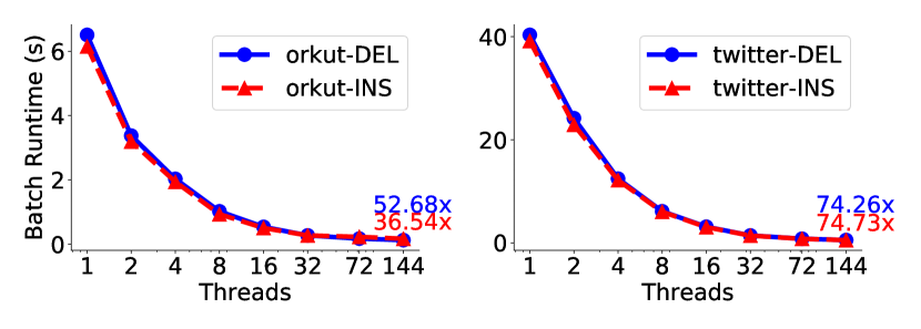
Figure 1: Running times of our parallel batch-dynamic triangle counting algorithm with respect to thread count (the $x$-axis is in log-scale) on the Orkut (average time across all batches) and Twitter (running time for the 6th batch) graph for both insertion (red dashed line) and deletion (blue solid line). “144” indicates 72 cores with hyper-threading. The experiment is run with a batch size of $2\times 10^{6}$. The parallel speedup on 144 threads over a single thread is displayed.

7.2 Comparison with Existing Algorithms

Comparison with Ediger et al. We compared our implementation with a shared-memory implementation of the Ediger et al. algorithm [EJRB10], which is implemented as part of the STINGER dynamic graph processing system [EMRB12]. Unfortunately, we found that their implementation is much slower than ours due to bottlenecks in the update time for the underlying dynamic graph data structure. We note that recent work on streaming graph processing observed similar results for using STINGER [DBS19]. To obtain a fair comparison, we chose to focus on implementing a more recent GPU batch-dynamic triangle counting algorithm ourselves, which we discuss next.

Comparison with Makkar et al. The Makkar et al. algorithm [MBG17] is a state-of-the-art parallel batch-dynamic triangle counting implementation designed for GPUs. To the best of our knowledge, there is no multicore implementation of this algorithm, and so in this paper we implement an optimized multicore version of their algorithm. The algorithm works as follows. First, their algorithm separates the batch of updates into batches for insertions and deletions. Then, for each batch of updates, it creates an update graph, $\hat{G}$, for each batch consisting of only the updates within each batch. Then, it merges the updates from each batch with the original edges in the graph to create an updated graph for each of the batches, $G^{\prime}$. Note that this graph contains both the edges previously in the graph, as well as the new edges.

The merging process to construct $G^{\prime}$ first sorts the batch to obtain sorted lists of neighbors to add/delete from the adjacency lists of vertices in the graph. Then, the algorithm performs a simple linear-work procedure to merge each existing adjacency list with the sorted updates. In particular, doing $t$ edge updates on a vertex with degree $d$ takes $O(d+t)$ work. Finally, the algorithm counts the triangles by intersecting the adjacency lists of the endpoints of each edge in the batch. For each edge $(u,v)$, they intersect $G^{\prime}(u)$ with $G^{\prime}(v)$, $G^{\prime}(u)$ with $\hat{G}(v)$, and $\hat{G}(u)$ with $\hat{G}(v)$. The count of the number of triangles can be obtained from the number of intersections obtained from each of these cases using a simple inclusion-exclusion formula. They provide a further optimization by only intersecting truncated adjacency lists in some of the cases where a truncated adjacency list is one where the list only contains vertices with IDs less than the ID of the vertex that the adjacency list belongs to. Their algorithm has a worst case work bound of $O(n^{2})$.

Implementation. We developed a new multicore implementation of the Makkar et al. algorithm using the same parallel primitives and framework described earlier for the implementation of our algorithm. We implemented several optimizations that improved performance. First, we handle vertices with degree lower than $16$ by storing their incident edges in a special array of size $16n$, and only allocate memory for vertices with larger degree. Second, we note that their algorithm does not specify how to handle redundant insertions that are already present in the graph. We remove these edge updates by modifying the merge algorithm that constructs $G^{\prime}$ from $G$. Specifically, during the merge, if we identify that a given edge is already present in $G$, we mark it in the sorted sequence of batch updates that we are merging in. Removing these marked updates to construct $\hat{G}$ without redundant updates is done by using a parallel filter.

Performance Comparison. Table 3 shows the running times of the Makkar et al. algorithm on batches of insertions and deletions of different sizes. The data points for the Twitter graph are also plotted in Figure 2. We observe that the Makkar et al. algorithm is faster than our algorithm on the Orkut graph, especially for large batches. On the other hand, for the Twitter graph, our algorithm is consistently faster for both insertions and deletions across all batch sizes. This is because there are no vertices with very high degree in the Orkut graph, and so the Makkar et al. algorithm does less work in merging adjacency lists with updates, while the Twitter graph has vertices with extremely high degree, which are costly to merge. Both algorithms are significantly faster than simply applying the static triangle counting algorithm for the range of batch sizes that we considered.

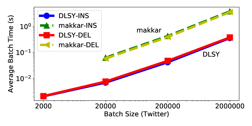
Figure 2: This figure plots the average insertion and deletion round times for each batch size (log-log scale) on Twitter using 72 cores with hyper-threading. The plot is in log-log scale. The lines for our algorithm are solid (blue for insertion and red for deletion) while the lines for Makkar et al. algorithm are dashed (green for insertion and yellow for deletion). The update time of Makkar et al. algorithm for Twitter batch size $2\times 10^{3}$ is missing because the experiment timed out (due to cumulative runtime being too large).

Next, we evaluate the performance of insertion batches in our algorithm and the Makkar et al. algorithm on the synthetic rMAT graph with 3.2 billion generated edges (which have duplicates). This synthetic experiment allows us to study how both algorithms perform as the graph becomes more dense. We evaluate the performance for different insertion batch sizes. The experiment uses prefixes of the rMAT graph (the number of unique edges per prefix is shown in Table 2) to control the density of the graph. The vertex set in this experiment is fixed, and thus a larger number of unique edges corresponds to a denser graph.

Figure 3 plots the running time of both implementations for varying batch sizes as a function of the graph density. We observe that for small batch sizes, the performance of the Makkar et al. algorithm degrades significantly as the graph grows more dense and contains more high-degree vertices. On the other hand, our algorithm’s performance generally does not degrade as the graph grows denser, across all batch sizes. We also significantly outperform the Makkar et al. algorithm for small batch sizes. Specifically, we obtain a maximum speedup of $3.31\times$ for a batch of size $2\times 10^{4}$. This is because the overhead of updating of high-degree vertices in the Makkar et al. algorithm becomes relatively higher, as work proportional to the vertex degree must be done regardless of the number of new incident edges.

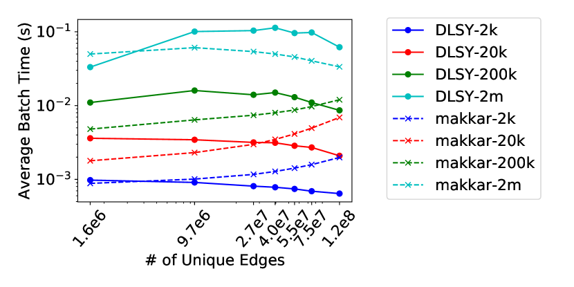
Figure 3: Comparison of the performance of our implementation (DLSY, solid line) and Makkar et al. algorithm [MBG17] (makkar, dotted line) for batches of insertions. The figure shows the average batch time for different batch sizes on the rMAT graph with varying prefixes of the generated edge stream to control density. The number of unique edges in the prefix is shown on the $x$-axis. The number of vertices is fixed at 16,384. The dark blue, red, green, and light blue lines are for batches of size $2\times 10^{3}$, $2\times 10^{4}$, $2\times 10^{5}$, and $2\times 10^{6}$, respectively. We see that our new algorithm is faster for small batches and on denser graphs.

8 Conclusion

In this paper, we have given new dynamic algorithms for the $k$-clique problem. We study this fundamental problem in the batch-dynamic setting, which is better suited for parallel hardware that is widely available today, and enables dynamic algorithms to scale to high-rate data streams. We have presented a work-efficient parallel batch-dynamic triangle counting algorithm. We also gave a simple, enumeration-based algorithm for maintaining the $k$-clique count. In addition, we have presented a novel parallel batch-dynamic $k$-clique counting algorithm based on fast matrix multiplication, which is asymptotically faster than existing dynamic approaches on dense graphs. Finally, we provide a multicore implementation of our parallel batch-dynamic triangle counting algorithm and compare it with state-of-the-art implementations that have weaker theoretical guarantees, showing that our algorithm is competitive in practice.

Acknowledgements. We thank Josh Alman, Nicole Wein, and Virginia Vassilevska Williams for helpful discussions on various aspects of our paper. We also thank anonymous reviewers for their helpful suggestions. This research was supported by DOE Early Career Award #DE-SC0018947, NSF CAREER Award #CCF-1845763, Google Faculty Research Award, DARPA SDH Award #HR0011-18-3-0007, and Applications Driving Architectures (ADA) Research Center, a JUMP Center co-sponsored by SRC and DARPA.

Appendix A Sequential Fully Dynamic Triangle Counting of [KNN⁺19]

Here, we present the sequential fully dynamic triangle counting algorithm of Kara et al. [KNN⁺19] that operates in $O(m)$ space, $O(\sqrt{m})$ amortized work per edge update, and $O(m^{3/2})$ work for preprocessing. This algorithm returns the exact count of the number of triangles in an undirected graph under both edge insertions and deletions. Kara et al. [KNN⁺19] present their algorithm for directed $3$-cycles using relational database terminology (where each edge in the triangle may be drawn from a different relation), but we simplify their algorithm for the case of undirected graphs. Kara et al. [KNN⁺19] prove the following theorem.

Theorem A.1 (Fully Dynamic Triangle Counting [KNN⁺19]).

There exists a sequential algorithm to count the number of triangles in an undirected graph $G=(V,E)$ using $O(m^{3/2})$ preprocessing work that can handle an edge update in $O(\sqrt{m})$ amortized work and $O(m)$ space.

We now explain the fully dynamic triangle counting algorithm of [KNN⁺19] in greater detail.

Given a graph $G=(V,E)$ with $n=|V|$ vertices and $m=|E|$ edges, we initialize the following variables: $M=2m+1$, $t_{1}=\sqrt{M}/2$, and $t_{2}=3\sqrt{M}/2$. We define a vertex to be low-degree if its degree is at most $t_{1}$ and high-degree if its degree is at least $t_{2}$. Vertices with degree in between $t_{1}$ and $t_{2}$ can be classified either way. Let $C$ be the current count of the number of triangles in the graph. We compute the initial count of the number of triangles in the input graph $G$ using a static triangle counting algorithm [IR77] in $O(m^{3/2})$ work and $O(m)$ space. Thus, we immediately have a preprocessing work of $O(m^{3/2})$.

We create four data structures $\mathcal{HH}$, $\mathcal{HL}$, $\mathcal{LH}$, and $\mathcal{LL}$. $\mathcal{HH}$ stores all of the edges $(u,v)$ where both $u$ and $v$ are high-degree, $\mathcal{HL}$ stores edges $(u,v)$, where $u$ is high-degree and $v$ is low-degree, $\mathcal{LH}$ stores the edges $(u,v)$ where $u$ is low-degree and $v$ is high-degree, and $\mathcal{LL}$ stores edges where both $u$ and $v$ are low-degree. With our data structures, the following operations are supported:

1. Given a vertex $v$, determine whether it is low-degree or high-degree in $O(1)$ work.

2. Given an edge $(u,v)$, check if it is in $\mathcal{HH}$, $\mathcal{HL}$, $\mathcal{LH}$, or $\mathcal{LL}$ in $O(1)$ work.

3. Given a vertex $v$, return all neighbors of $v$ in $\mathcal{HH}$, $\mathcal{HL}$, $\mathcal{LH}$, and $\mathcal{LL}$ in $O(\deg(v))$ work.

4. Given an edge $(v,w)$ to insert or delete, update $\mathcal{HH}$, $\mathcal{HL}$, $\mathcal{LH}$, or $\mathcal{LL}$ in $O(1)$ work.

We can implement $\mathcal{HH}$, $\mathcal{HL}$, $\mathcal{LH}$, and $\mathcal{LL}$ to support these operations by using a two-level hash table for each of these structures and an additional array $\mathcal{D}$. $\mathcal{D}$ is a dynamic hash table containing a key for each vertex that has non-zero degree and stores the degree of the vertex as the value. The data structures support insertions and deletions in $O(1)$ work. $\mathcal{D}$ can be initialized in $O(m)$ work by scanning over all vertices and computing their degree. $\mathcal{HH}$, $\mathcal{HL}$, $\mathcal{LH}$, and $\mathcal{LL}$ can be initialized in $O(m)$ work by scanning over all edges and inserting them into the right table based on the degrees of their endpoints.

We maintain one additional data structure $\mathcal{T}$ that counts the number of wedges $(u,w,v)$, where $u$ and $v$ are high-degree vertices and $w$ is a low-degree vertex. $\mathcal{T}$ has the property that given an edge insertion or deletion $(u,v)$ where both $u$ and $v$ are high-degree vertices, it returns the number of such wedges $(u,w,v)$ where $w$ is low-degree that $u$ and $v$ are part of in $O(1)$ work. We can implement this via a hash table indexed by pairs of high-degree vertices that stores the number of wedges for each pair. $\mathcal{T}$ can be initialized in $O(m^{3/2})$ work by iterating over all edges $(u,w)$ in $\mathcal{HL}$ and then for each $w$, iterating over all edges $(w,v)$ in $\mathcal{LH}$ to determine whether $v$ is high-degree, and if so then increment $T(u,v)$ by $1$. There are $O(m)$ edges $(u,w)$ in $\mathcal{HL}$, and for each $w$ there are at most $O(\sqrt{m})$ edges $(w,v)$ in $\mathcal{LH}$ since $w$ is low-degree. Each lookup and increment takes $O(1)$ work, giving an overall work of $O(m^{3/2})$.

A.1 Update Procedure [KNN⁺19]

The procedure for handling single edge updates in the sequential setting given by [KNN⁺19] as follows:

For an edge insertion (resp. deletion) $(u,v)$, we first find the degree of $u$ and $v$ in $\mathcal{D}$ and then look up the edge in their respective tables $\mathcal{HH}$, $\mathcal{HL}$, $\mathcal{LH}$, or $\mathcal{LL}$. If the edge already exists (resp. does not exist) in the table, nothing else is done. Otherwise, we need to find all tuples $(u,w,v)$ such that $(v,u)$ and $(u,w)$ already exist in the graph because for each such tuple, a new triangle will be formed (resp. an existing triangle will be deleted). We first update the triangle count, and then we update the data structures. For updating the triangle count $C$, there are $4$ different cases for such tuples, and so we check each of the following cases:

1. $(u,w)$ is in $\mathcal{HH}$ and $(w,v)$ is in $\mathcal{H}y$ where $y\in\{\mathcal{H},\mathcal{L}\}$: We extract all high-degree neighbors of $u$ in $\mathcal{HH}$. Given that the degree of all high-degree vertices is $\Omega(\sqrt{m})$, there are at most $O(\sqrt{m})$ such vertices. For each of these neighbors, we can check in $O(1)$ work for each $w$ whether $(w,v)$ exists in $\mathcal{H}y$. This takes $O(\sqrt{m})$ work.

2. $(u,w)$ is in $\mathcal{HL}$ and $(w,v)$ is in $\mathcal{LH}$ where $y\in\{\mathcal{H},\mathcal{L}\}$: Since both $u$ and $v$ are high-degree in this case, we perform an $O(1)$ work lookup in $\mathcal{T}$ for the count of the number of wedges $(u,w,v)$ in this case.

3. $(u,w)$ is in $\mathcal{LH}$ and $(w,v)$ is in $\mathcal{H}y$ where $y\in\{\mathcal{H},\mathcal{L}\}$: Scan through the neighbors of $u$ in $\mathcal{LH}$. For each neighbors of $u$, check whether $(w,v)$ exists in $\mathcal{H}y$. This takes $O(\sqrt{m})$ work since $u$ has low-degree.

4. $(u,w)$ is in $\mathcal{LL}$ and $(w,v)$ is in $\mathcal{L}y$ where $y\in\{\mathcal{L},\mathcal{H}\}$: Again, scan through the neighbors of $u$ in $\mathcal{LH}$. For each neighbors of $u$, check whether $(w,v)$ exists in $\mathcal{L}y$. This takes $O(\sqrt{m})$ work since $u$ has low-degree.

After updating the triangle count, we proceed with updating the data structures with the edge insertion (resp. deletion).

We first update $\mathcal{T}$ given an edge insertion (resp. deletion) $(u,v)$ as follows:

1. If $u$ is high-degree and $v$ is low-degree, then we find all of $v$’s neighbors in $\mathcal{LH}$ and for each such neighbor $x$, we increment (resp. decrement) the entry $\mathcal{T}(u,x)$ by $1$. It takes $O(\sqrt{m})$ work to perform this update since $v$ is low-degree.

2. If $u$ is low-degree and $v$ is high-degree, then we scan through all vertices in $\mathcal{HL}$ and for each vertex $x$ in $\mathcal{HL}$ that has $u$ as a neighbor, we increment (resp. decrement) $\mathcal{T}(x,v)$ by $1$. This takes $O(\sqrt{m})$ work since there are at most $O(\sqrt{m})$ high-degree vertices.

In addition to the updates to $\mathcal{T}$, we also insert (resp. delete) $(u,v)$ into $\mathcal{HH}$, $\mathcal{HL}$, $\mathcal{LH}$, and $\mathcal{LL}$ depending on the degrees of $u$ and $v$, and update $\mathcal{D}$. For a given edge $(u,v)$ insertion (resp. deletion), we first determine whether $u$ and $v$ are low-degree or high-degree by looking in $\mathcal{D}$ for $u$ and $v$ in $O(1)$ work. $\mathcal{HH}$, $\mathcal{HL}$, $\mathcal{LH}$, and $\mathcal{LL}$ are constructed as hash tables keyed by first the first vertex in the edge tuple and then the second vertex in the edge tuple with pointers to second-level hash tables storing the neighbors of that particular vertex. If $u$ is high-degree, then the edge is inserted (resp. deleted) into $\mathcal{HH}$ or $\mathcal{HL}$ (depending on whether $v$ is low or high-degree) using $u$ as the key and adding $v$ to the second level hash table. Similarly, if $u$ is low-degree, $(u,v)$ is inserted (resp. deleted) into $\mathcal{LH}$ or $\mathcal{LL}$. Furthermore, $(v,u)$ is also inserted into its respective table depending on whether $v$ is low or high-degree. The entries for $u$ and $v$ in $\mathcal{D}$ are then incremented (resp. decremented) in $\mathcal{D}$. The updates to these data structures take $O(1)$ work.

We also have to deal with the cases where the degree classification of vertices have changed or the number of edges has changed by too much that the values of $M$, $t_{1}$, and $t_{2}$ need to be updated. This is described in the next section.

A.2 Rebalancing [KNN⁺19]

We now describe the rebalancing procedure given in [KNN⁺19] when a low-degree vertex becomes a high-degree vertex (or vice versa) and when too many updates have been applied (and all the data structures must be changed according to the new values of $M$, $t_{1}$, and $t_{2}$).

Minor rebalancing. This type of rebalancing occurs if a vertex which was previously high-degree has its degree fall below $t_{1}$ or if a vertex that was previously low-degree has its degree increase above $t_{2}$. In the first case, we move the vertex and all its edges from $\mathcal{HH}$ to $\mathcal{HL}$, and from $\mathcal{LH}$ to $\mathcal{LL}$. In the second case, we move the vertex and all its edges from $\mathcal{HL}$ to $\mathcal{HH}$, and from $\mathcal{LL}$ to $\mathcal{LH}$. Since our data structures support additions and deletions of an edge in $O(1)$ work, and since the degree of $v$ is $\Theta(\sqrt{m})$ at this point, we perform $\Theta(\sqrt{m})$ updates. We showed in Section A.1 that updates take $O(\sqrt{m})$ work so we take $O(m)$ work overall for a minor rebalancing. However, $\Omega(\sqrt{m})$ updates must have occurred on this vertex before we have to perform minor rebalancing since $t_{2}-t_{1}=\Theta(\sqrt{m})$, and so we can amortize this cost over the $\Omega(\sqrt{m})$ updates, resulting in $O(\sqrt{m})$ amortized work per update.

Major rebalancing. A major rebalancing occurs when $m$, the number of edges in the graph, falls outside the range $[M/4,M]$. We simply reinitialize the data structures as in the original algorithm. Major rebalancing can only occur after $\Omega(M)$ updates, and so we can afford to re-initialize our data structure and recompute the triangle count from scratch using an $O(m^{3/2})$ work triangle counting algorithm. The amortized work of major rebalancing over $\Omega(m)$ updates is then $O(\sqrt{m})$.

References

- [AABD19] Umut A. Acar, Daniel Anderson, Guy E. Blelloch, and Laxman Dhulipala. Parallel batch-dynamic graph connectivity. In ACM Symposium on Parallelism in Algorithms and Architectures (SPAA), pages 381–392, 2019.
- [AAW17] Umut A. Acar, Vitaly Aksenov, and Sam Westrick. Brief announcement: Parallel dynamic tree contraction via self-adjusting computation. In ACM Symposium on Parallelism in Algorithms and Architectures (SPAA), pages 275–277, 2017.
- [AKM13] Shaikh Arifuzzaman, Maleq Khan, and Madhav Marathe. PATRIC: A parallel algorithm for counting triangles in massive networks. In ACM Conference on Information and Knowledge Management (CIKM), pages 529–538, 2013.
- [Alm19] Josh Alman. Linear Algebraic Techniques in Algorithms and Complexity. PhD thesis, Massachusetts Institute of Technology, 2019.
- [ALT+17] Christopher R. Aberger, Andrew Lamb, Susan Tu, Andres Nötzli, Kunle Olukotun, and Christopher Ré. EmptyHeaded: A relational engine for graph processing. ACM Trans. Database Syst., 42(4):20:1–20:44, 2017.
- [AMSJ18] Khaled Ammar, Frank McSherry, Semih Salihoglu, and Manas Joglekar. Distributed evaluation of subgraph queries using worst-case optimal low-memory dataflows. Proc. VLDB Endow., 11(6):691–704, February 2018.
- [ANR+17] Nesreen K. Ahmed, Jennifer Neville, Ryan A. Rossi, Nick G. Duffield, and Theodore L. Willke. Graphlet decomposition: framework, algorithms, and applications. Knowl. Inf. Syst., 50(3):689–722, 2017.
- [AOSS19] Sepehr Assadi, Krzysztof Onak, Baruch Schieber, and Shay Solomon. Fully dynamic maximal independent set with sublinear in update time. In ACM-SIAM Symposium on Discrete Algorithms, pages 1919–1936, 2019.
- [AW14] Amir Abboud and Virginia Vassilevska Williams. Popular conjectures imply strong lower bounds for dynamic problems. In IEEE Annual Symposium on Foundations of Computer Science (FOCS), page 434–443, 2014.
- [AYZ97] N. Alon, R. Yuster, and U. Zwick. Finding and counting given length cycles. Algorithmica, 17(3):209–223, Mar 1997.
- [BAD20] Guy E. Blelloch, Daniel Anderson, and Laxman Dhulipala. Brief announcement: ParlayLib – a toolkit for parallel algorithms on shared-memory multicore machines. In ACM Symposium on Parallelism in Algorithms and Architectures (SPAA), pages 507–509, 2020.
- [BCH19] Matthias Bonne and Keren Censor-Hillel. Distributed detection of cliques in dynamic networks. In International Colloquium on Automata, Languages, and Programming (ICALP 2019), pages 132:1–132:15, 2019.
- [BE10] Leonid Barenboim and Michael Elkin. Sublogarithmic distributed MIS algorithm for sparse graphs using Nash-Williams decomposition. Distributed Computing, 22(5):363–379, Aug 2010.
- [BKM19] Philipp Bamberger, Fabian Kuhn, and Yannic Maus. Local distributed algorithms in highly dynamic networks. In IEEE International Parallel and Distributed Processing Symposium (IPDPS), pages 33–42, 2019.
- [Blä13] Markus Bläser. Fast matrix multiplication. Theory of Computing, Graduate Surveys, 5:1–60, 2013.
- [CHDK+19] Keren Censor-Hillel, Neta Dafni, Victor I Kolobov, Ami Paz, and Gregory Schwartzman. Fast and simple deterministic algorithms for highly-dynamic networks. arXiv preprint arXiv:1901.04008, 2019.
- [CHHK16] Keren Censor-Hillel, Elad Haramaty, and Zohar Karnin. Optimal dynamic distributed MIS. In ACM Symposium on Principles of Distributed Computing, pages 217–226, 2016.
- [CN85] Norishige Chiba and Takao Nishizeki. Arboricity and subgraph listing algorithms. SIAM J. Comput., 14(1):210–223, February 1985.
- [CZF04] Deepayan Chakrabarti, Yiping Zhan, and Christos Faloutsos. R-mat: A recursive model for graph mining. In SIAM International Conference on Data Mining (SDM), pages 442–446, 2004.
- [DAH17] V. S. Dave, N. K. Ahmed, and M. Hasan. PE-CLoG: Counting edge-centric local graphlets. In IEEE International Conference on Big Data, pages 586–595, 2017.
- [DBS18a] Maximilien Danisch, Oana Balalau, and Mauro Sozio. Listing -cliques in sparse real-world graphs. In International Conference on World Wide Web (WWW), pages 589–598, 2018.
- [DBS18b] Laxman Dhulipala, Guy E. Blelloch, and Julian Shun. Theoretically efficient parallel graph algorithms can be fast and scalable. In ACM Symposium on Parallelism in Algorithms and Architectures (SPAA), pages 393–404, 2018.
- [DBS19] Laxman Dhulipala, Guy E Blelloch, and Julian Shun. Low-latency graph streaming using compressed purely-functional trees. In ACM SIGPLAN Conference on Programming Language Design and Implementation (PLDI), pages 918–934, 2019.
- [DDK+20] Laxman Dhulipala, David Durfee, Janardhan Kulkarni, Richard Peng, Saurabh Sawlani, and Xiaorui Sun. Parallel batch-dynamic graphs: Algorithms and lower bounds. In ACM-SIAM Symposium on Discrete Algorithms (SODA), pages 1300–1319, 2020.
- [DF94] Sajal K. Das and Paolo Ferragina. An work EREW parallel algorithm for updating MST. In Annual European Symposium on Algorithms (ESA), pages 331–342, 1994.
- [DF95] Rod G. Downey and Michael R. Fellows. Fixed-parameter tractability and completeness I: Basic results. SIAM Journal on Computing, 24(4):873–921, 1995.
- [DT13] Zdeněk Dvořák and Vojtěch Tůma. A dynamic data structure for counting subgraphs in sparse graphs. In Algorithms and Data Structures, pages 304–315, 2013.
- [EG04] Friedrich Eisenbrand and Fabrizio Grandoni. On the complexity of fixed parameter clique and dominating set. Theor. Comput. Sci., 326(1-3):57–67, October 2004.
- [EGST12] David Eppstein, Michael T. Goodrich, Darren Strash, and Lowell Trott. Extended dynamic subgraph statistics using -index parameterized data structures. Theoretical Computer Science, 447:44 – 52, 2012.
- [EJRB10] D. Ediger, K. Jiang, J. Riedy, and D. A. Bader. Massive streaming data analytics: A case study with clustering coefficients. In IEEE International Symposium on Parallel Distributed Processing, Workshops and PhD Forum (IPDPSW), pages 1–8, 2010.
- [EMRB12] David Ediger, Robert McColl, Jason Riedy, and David A Bader. Stinger: High performance data structure for streaming graphs. In IEEE Conference on High Performance Extreme Computing (HPEC), pages 1–5, 2012.
- [ES09] David Eppstein and Emma S. Spiro. The -index of a graph and its application to dynamic subgraph statistics. In Algorithms and Data Structures (WADS), pages 278–289, 2009.
- [ESBD16] Ethan R. Elenberg, Karthikeyan Shanmugam, Michael Borokhovich, and Alexandros G. Dimakis. Distributed estimation of graph 4-profiles. In International Conference on World Wide Web (WWW), pages 483–493, 2016.
- [FFF15] Irene Finocchi, Marco Finocchi, and Emanuele G. Fusco. Clique counting in MapReduce: Algorithms and experiments. J. Exp. Algorithmics, 20:1.7:1–1.7:20, October 2015.
- [FL94] Paolo Ferragina and Fabrizio Luccio. Batch dynamic algorithms for two graph problems. In Parallel Architectures and Languages Europe (PARLE), pages 713–724, 1994.
- [GMV91] J. Gil, Y. Matias, and U. Vishkin. Towards a theory of nearly constant time parallel algorithms. In IEEE Symposium on Foundations of Computer Science (FOCS), pages 698–710, 1991.
- [GP11] Michael T. Goodrich and Paweł Pszona. External-memory network analysis algorithms for naturally sparse graphs. In European Symposium on Algorithms, ESA’11, page 664–676, 2011.
- [Gra] GraphChallenge. http://graphchallenge.mit.edu/.
- [Gra77] Mark S Granovetter. The strength of weak ties. In Social Networks, pages 347–367. Elsevier, 1977.
- [HD14] Tomaz Hocevar and Janez Demsar. A combinatorial approach to graphlet counting. Bioinformatics, pages 559–65, 2014.
- [HR05] Robert A. Hanneman and Mark Riddle. Introduction to Social Network Methods. University of California, Riverside, 2005.
- [ILMP19] Giuseppe F. Italiano, Silvio Lattanzi, Vahab S. Mirrokni, and Nikos Parotsidis. Dynamic algorithms for the massively parallel computation model. In ACM Symposium on Parallelism in Algorithms and Architectures (SPAA), pages 49–58, 2019.
- [IR77] Alon Itai and Michael Rodeh. Finding a minimum circuit in a graph. In Annual ACM Symposium on Theory of Computing (STOC), pages 1–10, 1977.
- [Jaj92] J. Jaja. Introduction to Parallel Algorithms. Addison-Wesley Professional, 1992.
- [JS17] Shweta Jain and C. Seshadhri. A fast and provable method for estimating clique counts using Turán’s theorem. In International Conference on World Wide Web (WWW), pages 441–449, 2017.
- [Kha17] Shahbaz Khan. Near optimal parallel algorithms for dynamic DFS in undirected graphs. In ACM Symposium on Parallelism in Algorithms and Architectures (SPAA), pages 283–292, 2017.
- [KLPM10] Haewoon Kwak, Changhyun Lee, Hosung Park, and Sue Moon. What is twitter, a social network or a news media? pages 591–600, 2010.
- [KNN+19] Ahmet Kara, Hung Q. Ngo, Milos Nikolic, Dan Olteanu, and Haozhe Zhang. Counting triangles under updates in worst-case optimal time. In International Conference on Database Theory (ICDT), volume 127, pages 4:1–4:18, 2019.
- [KPR18] Tsvi Kopelowitz, Ely Porat, and Yair Rosenmutter. Improved worst-case deterministic parallel dynamic minimum spanning forest. In ACM Symposium on Parallelism in Algorithms and Architectures (SPAA), pages 333–341, 2018.
- [Lat08] Matthieu Latapy. Main-memory triangle computations for very large (sparse (power-law)) graphs. Theor. Comput. Sci., 407(1-3):458–473, 2008.
- [LG14] François Le Gall. Powers of tensors and fast matrix multiplication. In International Symposium on Symbolic and Algebraic Computation (ISSAC), pages 296–303, 2014.
- [LK14] Jure Leskovec and Andrej Krevl. SNAP Datasets: Stanford large network dataset collection. 2014.
- [MBG17] D. Makkar, D. A. Bader, and O. Green. Exact and parallel triangle counting in dynamic graphs. In IEEE International Conference on High Performance Computing (HiPC), pages 2–12, Dec 2017.
- [New03] Mark EJ Newman. The structure and function of complex networks. SIAM review, 45(2):167–256, 2003.
- [NP85] Jaroslav Nešetřil and Svatopluk Poljak. On the complexity of the subgraph problem. Commentationes Mathematicae Universitatis Carolinae, 026(2):415–419, 1985.
- [NPRR18] Hung Q. Ngo, Ely Porat, Christopher Ré, and Atri Rudra. Worst-case optimal join algorithms. J. ACM, 65(3):16:1–16:40, March 2018.
- [PC13] Ha-Myung Park and Chin-Wan Chung. An efficient MapReduce algorithm for counting triangles in a very large graph. In ACM Conference on Information and Knowledge Management (CIKM), pages 539–548, 2013.
- [PSKP14] Ha-Myung Park, Francesco Silvestri, U Kang, and Rasmus Pagh. MapReduce triangle enumeration with guarantees. In ACM Conference on Information and Knowledge Management (CIKM), 2014.
- [PSV17] Ali Pinar, C. Seshadhri, and Vaidyanathan Vishal. ESCAPE: Efficiently counting all 5-vertex subgraphs. In International Conference on World Wide Web (WWW), pages 1431–1440, 2017.
- [RT94] John H. Reif and Stephen R. Tate. Dynamic parallel tree contraction (extended abstract). In ACM Symposium on Parallel Algorithms and Architectures (SPAA), pages 114–121, 1994.
- [SB14] Julian Shun and Guy E Blelloch. Phase-concurrent hash tables for determinism. In ACM Symposium on Parallelism in Algorithms and Architectures (SPAA), pages 96–107, 2014.
- [SBF+12] Julian Shun, Guy E. Blelloch, Jeremy T. Fineman, Phillip B. Gibbons, Aapo Kyrola, Harsha Vardhan Simhadri, and Kanat Tangwongsan. Brief announcement: the Problem Based Benchmark Suite. In ACM Symposium on Parallelism in Algorithms and Architectures (SPAA), pages 68–70, 2012.
- [Sch93] Marco Schneider. Self-stabilization. ACM Computing Surveys (CSUR), 25(1):45–67, 1993.
- [SDS20] Jessica Shi, Laxman Dhulipala, and Julian Shun. Parallel clique counting and peeling algorithms. CoRR, abs/2002.10047, 2020.
- [ST15] Julian Shun and Kanat Tangwongsan. Multicore triangle computations without tuning. In IEEE International Conference on Data Engineering (ICDE), pages 149–160, 2015.
- [STTW18] Natcha Simsiri, Kanat Tangwongsan, Srikanta Tirthapura, and Kun-Lung Wu. Work-efficient parallel union-find. Concurrency and Computation: Practice and Experience, 30(4), 2018.
- [SV11] Siddharth Suri and Sergei Vassilvitskii. Counting triangles and the curse of the last reducer. In International Conference on World Wide Web (WWW), pages 607–614, 2011.
- [TDB19] Thomas Tseng, Laxman Dhulipala, and Guy E. Blelloch. Batch-parallel Euler tour trees. In Workshop on Algorithm Engineering and Experiments (ALENEX), pages 92–106, 2019.
- [Vas09] Virginia Vassilevska. Efficient algorithms for clique problems. Information Processing Letters, 109(4):254–257, 2009.
- [Vis10] Uzi Vishkin. Thinking in parallel: Some basic data-parallel algorithms and techniques. 2010.
- [Wil12] Virginia Vassilevska Williams. Multiplying matrices faster than Coppersmith-Winograd. In ACM Symposium on Theory of Computing Conference (STOC), pages 887–898, 2012.
- [WS98] Duncan J Watts and Steven H Strogatz. Collective dynamics of ‘small-world’ networks. Nature, 393(6684):440, 1998.